1 Introduction
The process of recovering oil from a reservoir traditionally comprises three stages. When first drilling into a reservoir, the high pressure in the rock forces out hydrocarbons in the form of gases and oils; this process is referred to as primary oil recovery. Eventually, the naturally high pressure in the reservoir drops, and water needs to be injected to maintain the rate at which the oil is retrieved. Typically, seawater is used for this secondary water-flood. However, a high percentage of the oil remains undisturbed, and a tertiary water-flood is often performed to remove some of the oil that cannot be recovered using seawater alone. Numerous technologies have been developed for this tertiary recovery stage, such as alkaline flooding, polymer flooding and gas injection. This paper is motivated by one such technology, namely low-salinity water-flooding.
In low-salinity water-flooding, low-salinity water, rather than seawater, is injected into the reservoir. Provided certain conditions are met, such as polar compounds being present in the oil, clay compounds being present in the reservoir and divalent ions being present in the formation water (water naturally residing in the oil reservoir before any water-flooding has taken place), a low-salinity water-flood results in additional oil being recovered (Austad, RezaeiDoust & Puntervold Reference Austad, Rezaeidoust and Puntervold2010). While the requirements for low-salinity oil recovery to be effective are relatively well known, the dominant causal mechanism is not well understood, and a number of potential mechanisms have been proposed in the literature.
Morrow (Reference Morrow1990) suggests that the presence of lower-salinity water causes the electrical double layer between the clay platelets present in the reservoir to expand and release fines. These fines act as a surfactant, and alter the permeability of the reservoir. McGuire et al. (Reference McGuire, Chatham, Paskvan, Sommer and Carini2005) suggest that, due to the increase in pH during a low-salinity injection, the interfacial tension is reduced, leading to a wettability alteration. As a secondary effect, they claim that the carboxylic compounds in the oil are desorbed from the clay as a result of the pH increase.
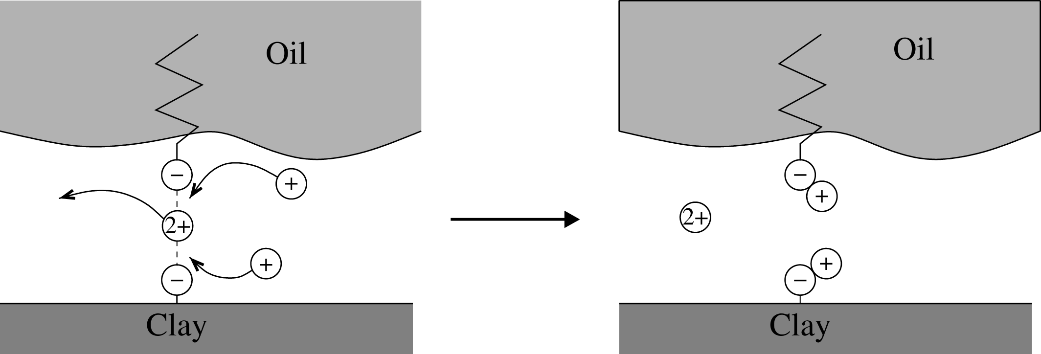
Lager et al. (Reference Lager, Webb, Black, Singleton and Sorbie2008) propose an alternative mechanism, known as multicomponent ionic exchange (MIE). In this mechanism, divalent cations residing in the formation water attract oil to the clay by forming a bridge across the thin film of water separating the oil and the clay, binding the negatively charged carboxylate ions on the oil surface to the negatively charged exchange sites on the clay surface. Lager et al. (Reference Lager, Webb, Black, Singleton and Sorbie2008) assert that, as the concentration of divalent ions in the injected water is decreased, the ions attracting the oil to the clay migrate into the bulk liquid, and are replaced by monovalent ions, allowing the release of oil. A schematic diagram of the MIE process is shown in figure 1. Additionally, they claim that the thin film of water between the oil and clay expands in the low-salinity regime, due to electric double-layer expansion, reducing the attraction of the oil to the clay surface, and thus assisting the release of oil.
Schematic diagram of the multicomponent ionic exchange (MIE) mechanism.

Numerous experimental studies have been undertaken to distinguish between these different mechanisms. The majority of these are core-scale experiments, in which a sample of reservoir rock, a ‘core’, approximately
 $10~\text{cm}\times 4~\text{cm}^{2}$
, is water-flooded with brine (Jadhunandan Reference Jadhunandan1990; Jadhunandan & Morrow Reference Jadhunandan and Morrow1991, Reference Jadhunandan and Morrow1995; Yildiz Reference Yildiz1995; Yildiz & Morrow Reference Yildiz and Morrow1996; Lager et al.
Reference Lager, Webb, Black, Singleton and Sorbie2008; Ligthelm et al.
Reference Ligthelm, Gronsveld, Hofman, Brussee, Marcelis and van der Linde2009; RezaeiDoust, Puntervold & Austad Reference RezaeiDoust, Puntervold and Austad2011). By studying the amount of oil produced during core experiments, and the composition of the brine produced at the outlet, for different oil, rock and inlet brine compositions, these experiments provide a good understanding of the requirements for effective low-salinity oil recovery.
By performing core-scale experiments, Lager et al. (Reference Lager, Webb, Black, Singleton and Sorbie2008) observe that a greater oil recovery can be achieved without any increase in the number of fines produced, or any significant permeability alteration, and thus they assert that fines migration is unlikely to be the dominant mechanism. They also dispute the pH increase mechanism, as low-salinity effects were observed in experiments in which the pH only showed a slight increase.
As an alternative to a core experiment, Berg et al. (Reference Berg, Cense, Jansen and Bakker2010) pass water over oil on a clay surface and demonstrate the weakening of the adhesion forces between oil droplets and a clay surface in the low-salinity regime. They observe that the oil droplets lift from the clay surface as the salinity of the surrounding fluid reduces. These results support the MIE mechanism proposed by Lager et al. (Reference Lager, Webb, Black, Singleton and Sorbie2008).
A key component in the MIE mechanism is the expansion of the thin water film between the oil and clay. Lee et al. (Reference Lee, Webb, Collins, Lager, Clarke, O’Sullivan, Routh and Wang2010) used small-angle neutron scattering to measure the thickness of the film,
 $h^{\ast }$
, for various salinities, and found that
 $h^{\ast }$
varies from 0.9 nm in the high-salinity regime to 1.3 nm in the low-salinity regime. These results support the MIE mechanism by demonstrating the increase in the film thickness as a result of double-layer expansion and the weakening of adhesion forces at the oil–clay interface during a low-salinity water-flood.
Theoretical predictions for the thickness of the thin layer of water between the clay and the oil have been made by balancing the capillary pressure and electro-osmotic pressure (Hirasaki Reference Hirasaki1991; Wong, Morris & Radke Reference Wong, Morris and Radke1992; Kovscek, Wong & Radke Reference Kovscek, Wong and Radke1993). These forces are derived from the Derjaguin–Verwey–Landau–Overbeek (DVLO) theory of colloidal stability (Derjaguin & Landau Reference Derjaguin and Landau1941; Verwey & Overbeek Reference Verwey and Overbeek1948), in which the disjoining pressure,
 $\unicode[STIX]{x1D6F1}$
, is taken to be the same as between two flat plates (Parsegian & Gingell Reference Parsegian and Gingell1972; Ohshima Reference Ohshima1974a
,Reference Ohshima
b
; McCormack, Carnie & Chan Reference McCormack, Carnie and Chan1995; Ben-Yaakov & Andelman Reference Ben-Yaakov and Andelman2010). However, there does not appear to be a systematic derivation of the height at which the oil lies above the clay when the oil–water interface is treated as a free surface. Further, the expressions often stated for the film thickness are for static models (Hirasaki Reference Hirasaki1991; Wong et al.
Reference Wong, Morris and Radke1992; Kovscek et al.
Reference Kovscek, Wong and Radke1993; Kuchin et al.
Reference Kuchin, Matar, Craster and Starov2014a
,Reference Kuchin, Matar, Craster and Starov
b
). However, as can be seen by studying the motion of bubbles through capillary tubes (Bretherton Reference Bretherton1961; Wong, Radke & Morris Reference Wong, Radke and Morris1995a
,Reference Wong, Radke and Morris
b
), or by studying the spreading of droplets on surfaces (Tanner Reference Tanner1979), the film thickness below a moving droplet is dependent on the velocity at which the droplet moves. Hence these static models are of limited use when studying oil motion through a pore space.
The motion of a fluid through a prewetted capillary in the presence of a disjoining pressure has been previously studied, for example, in Starov, Kalinin & Ivanov (Reference Starov, Kalinin and Ivanov1994) and Egorov, Kornev & Neimark (Reference Egorov, Kornev and Neimark2003). However, these authors do not include the electrostatic effects of charged surfaces. On the other hand, Kuchin et al. (Reference Kuchin, Matar, Craster and Starov2014a ,Reference Kuchin, Matar, Craster and Starov b ) study the profile of a capillary meniscus with the inclusion of electrostatic effects. However, in their model the meniscus is static, and so they do not consider Bretherton effects, which will influence the motion of oil.
In this paper, we study the paradigm problem of the two-dimensional steady motion of a charged oil slug in a charged pore throat, where the surrounding water contains both monovalent and divalent ions. Our aim is to determine the speed at which an oil slug moves through a pore throat as a function of the salinity of the surrounding brine, assuming that the MIE reactions occur on the surfaces of the oil and the pore. An increase in the velocity of oil in a reservoir can lead to a greater oil recovery, both per unit time and in total, since the faster-moving oil in the low-salinity region catches up with the slower-moving oil ahead of the low-salinity front. This results in increased connectivity of the oil phase, which leads to a reduction in the residual oil. Thus, by studying this problem, we can determine whether the MIE mechanism is likely to be responsible for the increased oil recovery observed during a low-salinity water-flood. We note though that flow through a porous structure also depends on the pressure required to drive the oil droplets into the throat from the pore body. Cobos, Carvalho & Alvarado (Reference Cobos, Carvalho and Alvarado2009) studied the flow of two oil-in-water emulsions through a converging–diverging capillary tube. They found that, for emulsions in which the droplet size is larger than the narrowest section of the capillary, the flow is dominated by a blocking mechanism. Larger-scale models (over many pores) of the MIE mechanism would therefore need to include the effect of entry pressure.
In § 2, we will present a mathematical model to describe the motion of the oil slug, which includes a simple model for the reactions occurring between the ions and the oil and clay surfaces. The MIE reactions affect the surface charge densities of the oil–water and clay–water interfaces, which, in turn, affect the electrical component of the force acting between them. In § 3, we will find the electric potential inside the capillary as a function of the surface charge densities, as this is needed to determine how the thickness of the water film separating the oil slug from the clay surface depends on the salinity of the surrounding brine.
In § 4, we will determine the film thickness between the oil and clay surfaces as a function of the surface charge densities, and we will also determine the radii of curvature of the front and rear ends of the oil slug. We will then study the macroscopic flow problem to derive an expression for the velocity at which the oil slug moves given a pressure difference along the length of the pore throat. On this scale, the water film becomes an effective partial slip boundary condition on the oil–clay interface, with the slip length determined by the film thickness. The front and rear menisci radii affect the pressure drop felt by the oil slug, and thus the speed at which it moves through the pore. We will solve the model assuming that the ratio of the pressure drop to the disjoining pressure due to the charged surfaces is
 $O(1)$
, and we will compare the results with the asymptotic solution in the limit in which this term tends to zero. Finally, in § 5, we will draw together our findings and discuss their application.
2 Model formulation
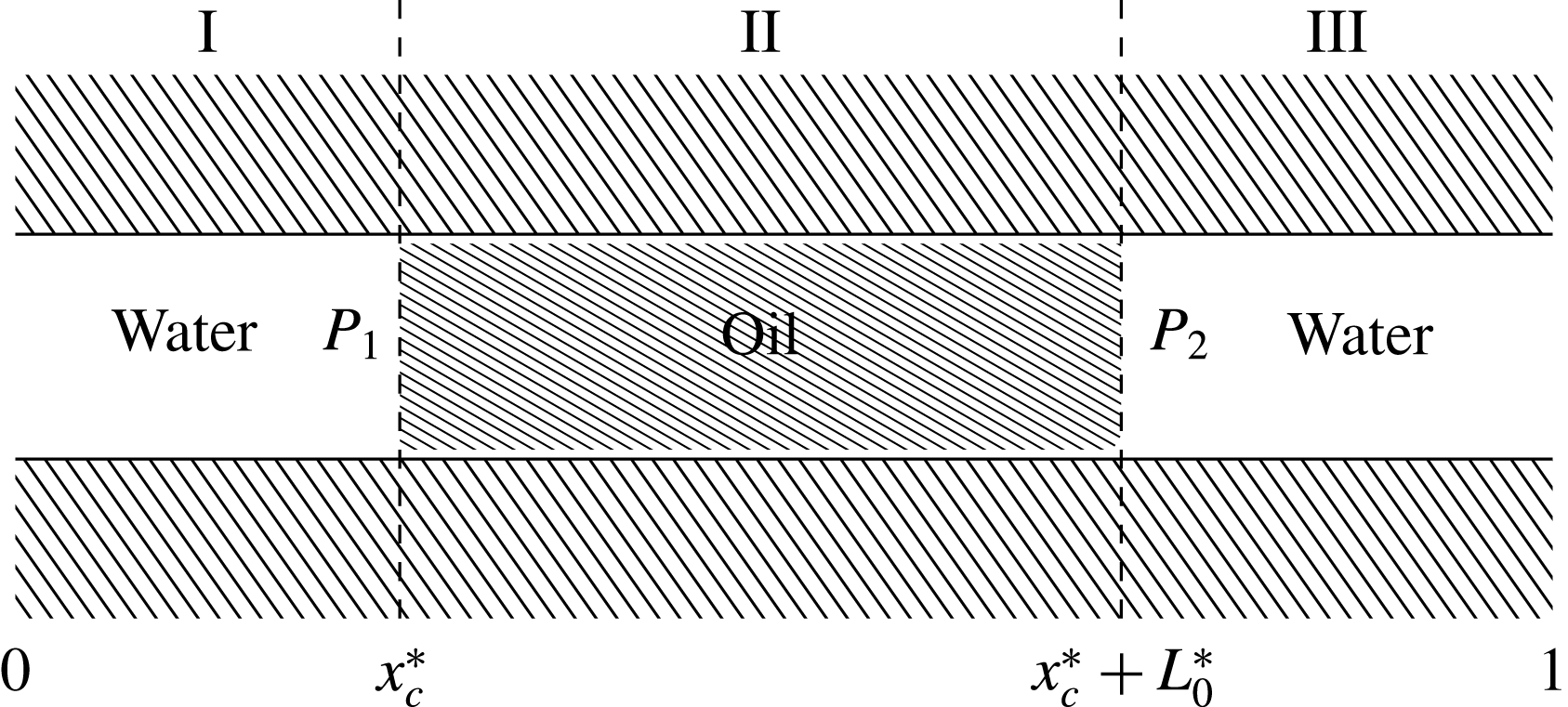
We wish to model the motion of an oil slug through a clay pore throat filled with saline water, subject to a constant pressure difference,
 $P$
, across the ends of the pore. We suppose that the pore throat can be represented by a two-dimensional capillary tube of length
 $L$
and height
 $2R$
, and that at each end of the capillary there is a bulk region of water. We label the oil region by
 $\unicode[STIX]{x1D6FA}_{o}$
, the surrounding water region by
 $\unicode[STIX]{x1D6FA}_{w}$
, and the clay regions bounding either side of the capillary tube by
 $\unicode[STIX]{x1D6FA}_{c}$
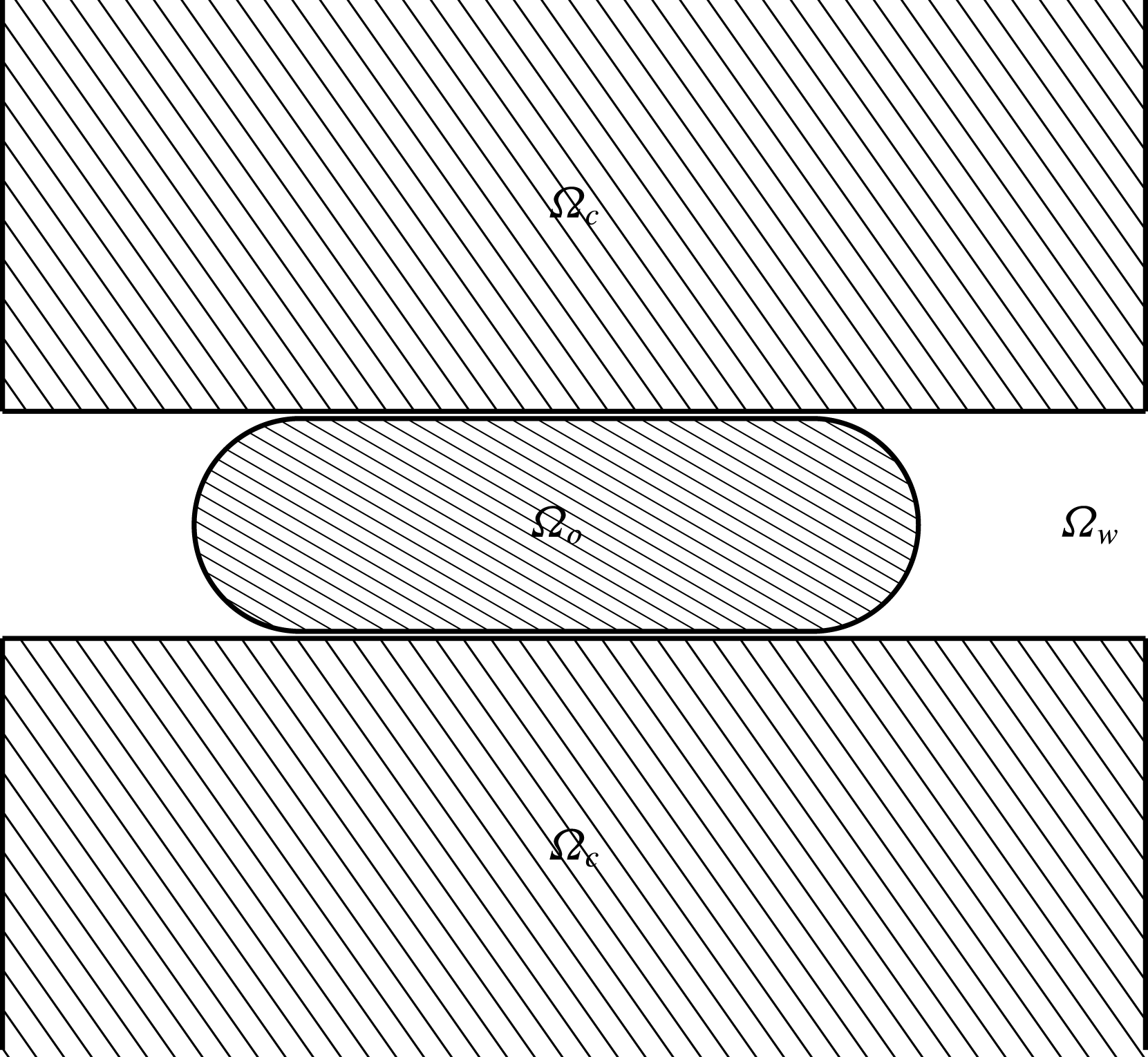
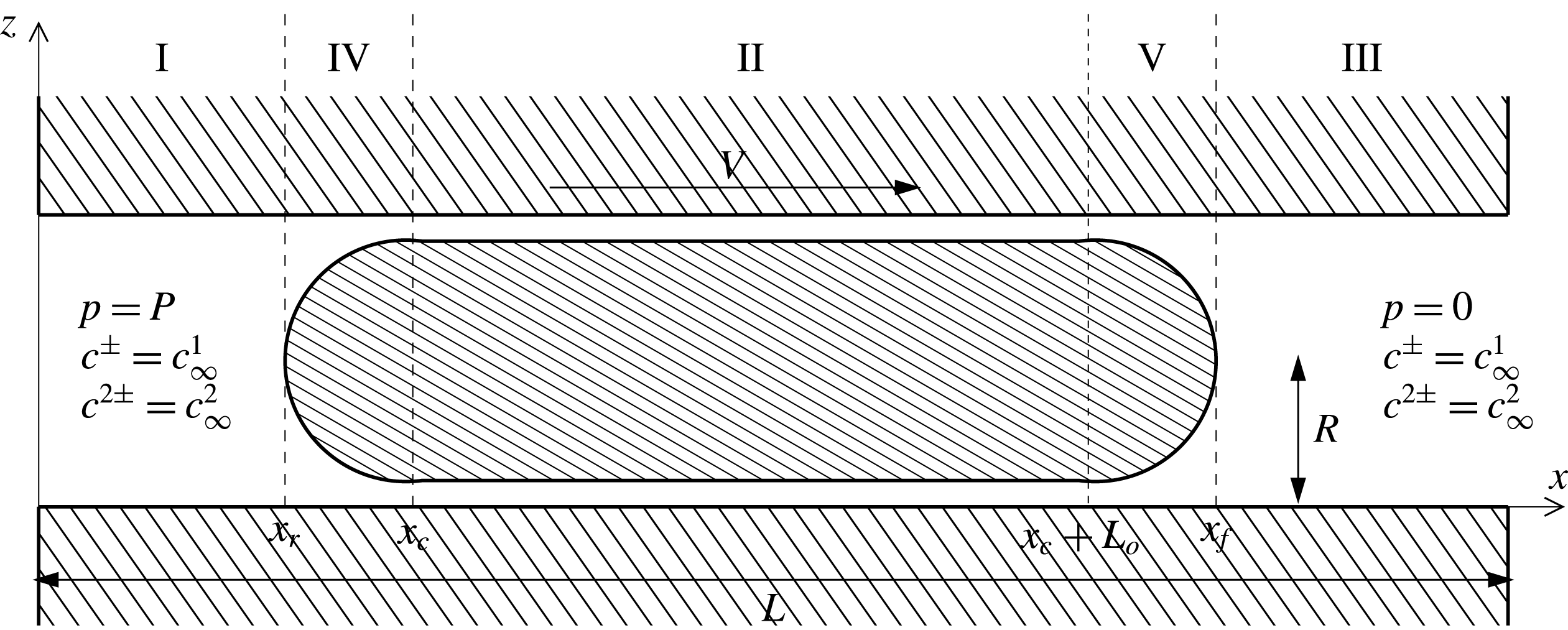
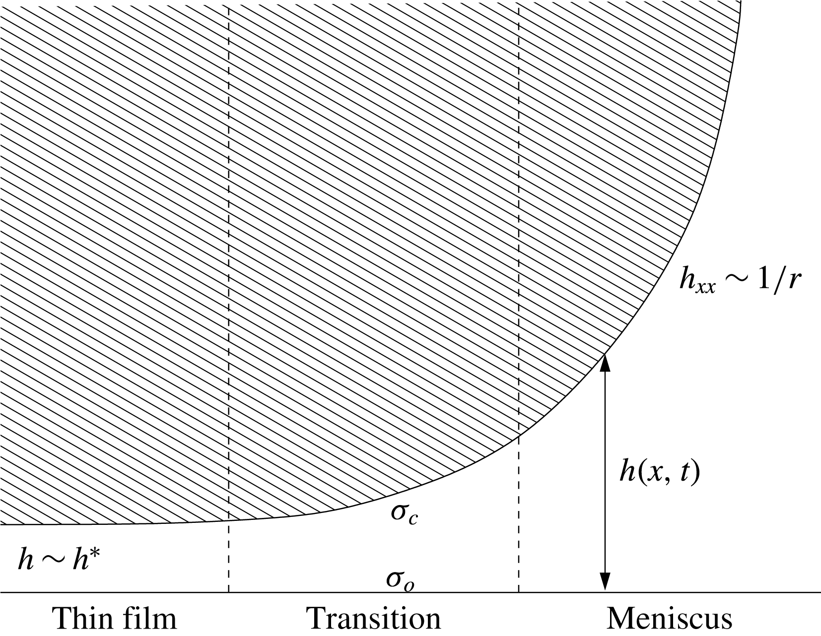
, as shown in figure 2. We assume that there is a thin film of water separating the oil from the clay surface (due to electrostatic and viscous effects) along the upper and lower surfaces of the oil slug. The thickness of this water layer is unknown a priori; however, we assume that it is thin enough such that, from a macroscopic perspective, there appears to be contact between the oil and the clay. We denote the length of the oil droplet, measured from the apparent contact point of the rear meniscus to the apparent contact point of the front meniscus, by
 $L_{o}$
, and we assume that
 $L_{o}=O(L)$
. Taking the origin of our coordinate system to be the lower left corner of the tube, we suppose that the rear apparent contact point has horizontal coordinate
 $x_{c}$
, with the extremal positions of the front and rear menisci being
 $x_{f}$
and
 $x_{r}$
, as shown in figure 3.
In order to model the effect of the salinity of the water on the motion of the oil slug, we assume that the water phase contains solvated positively and negatively charged ions, with the concentrations of the monovalent and divalent species being
 $c^{\pm }$
and
 $c^{2\pm }$
, respectively. In order to model ion exchange mechanisms on the capillary wall, and on the oil–water interface, we assume that these surfaces contain a number of negatively charged exchange sites at which reactions are allowed to occur.
Schematic diagram of the macroscopic motion of an oil slug through a capillary between two bulk phases of water.

Schematic diagram of the capillary problem. The thickness of the water layer below the oil slug has been exaggerated for illustrative purposes.

2.1 Governing equations
We model the oil and water using the Navier–Stokes equations. Owing to the presence of the ions, the net charge density is
 $q(c^{+}-c^{-}+2c^{2+}-2c^{2-})$
in the water phase, where
 $q$
is the (absolute) charge of an electron. Hence, the electric field,
 $-\unicode[STIX]{x1D735}\unicode[STIX]{x1D719}$
, induces a force on the water, and we have to include this body force in the equations for the water phase (Yang, Fu & Hwang Reference Yang, Fu and Hwang2001; Waghmare & Mitra Reference Waghmare and Mitra2008). Thus we write
 $$\begin{eqnarray}\displaystyle & \displaystyle \unicode[STIX]{x1D735}\boldsymbol{\cdot }\boldsymbol{u}_{w}=0,\quad \text{in }\unicode[STIX]{x1D6FA}_{w}, & \displaystyle\end{eqnarray}$$
 $$\begin{eqnarray}\displaystyle & \displaystyle \unicode[STIX]{x1D70C}_{w}\frac{\text{D}\boldsymbol{u}_{w}}{\text{D}t}=-\unicode[STIX]{x1D735}p_{w}+\unicode[STIX]{x1D707}_{w}\unicode[STIX]{x1D6FB}^{2}\boldsymbol{u}_{w}-q(c^{+}-c^{-}+2c^{2+}-2c^{2-})\unicode[STIX]{x1D735}\unicode[STIX]{x1D719},\quad \text{in }\unicode[STIX]{x1D6FA}_{w}, & \displaystyle\end{eqnarray}$$
 $$\begin{eqnarray}\displaystyle & \displaystyle \unicode[STIX]{x1D735}\boldsymbol{\cdot }\boldsymbol{u}_{o}=0,\quad \text{in }\unicode[STIX]{x1D6FA}_{o}, & \displaystyle\end{eqnarray}$$
 $$\begin{eqnarray}\displaystyle & \displaystyle \unicode[STIX]{x1D70C}_{o}\frac{\text{D}\boldsymbol{u}_{o}}{\text{D}t}=-\unicode[STIX]{x1D735}p_{o}+\unicode[STIX]{x1D707}_{o}\unicode[STIX]{x1D6FB}^{2}\boldsymbol{u}_{o},\quad \text{in }\unicode[STIX]{x1D6FA}_{o}, & \displaystyle\end{eqnarray}$$
where
 $\boldsymbol{u}_{w}=(u_{w},w_{w})$
is the velocity in the water phase,
 $\boldsymbol{u}_{o}=(u_{o},w_{o})$
is the velocity in the oil phase,
 $p_{w}$
,
 $\unicode[STIX]{x1D70C}_{w}$
and
 $\unicode[STIX]{x1D707}_{w}$
are the pressure, density and viscosity of the water, respectively, while
 $p_{o}$
,
 $\unicode[STIX]{x1D70C}_{o}$
and
 $\unicode[STIX]{x1D707}_{o}$
are the pressure, density and viscosity of the oil, respectively,
 $\unicode[STIX]{x1D719}$
is the electric potential and
 $\text{D}/\text{D}t=\unicode[STIX]{x2202}/\unicode[STIX]{x2202}t+\boldsymbol{u}\boldsymbol{\cdot }\unicode[STIX]{x1D735}$
is the advective derivative.
The ion concentrations are governed by the Nernst–Planck (drift–diffusion) equations,
 $$\begin{eqnarray}\displaystyle & \displaystyle \frac{\unicode[STIX]{x2202}c^{\pm ,2\pm }}{\unicode[STIX]{x2202}t}=-\unicode[STIX]{x1D735}\boldsymbol{\cdot }\boldsymbol{J}^{\pm ,2\pm },\quad \text{in }\unicode[STIX]{x1D6FA}_{w}, & \displaystyle\end{eqnarray}$$
 $$\begin{eqnarray}\displaystyle & \displaystyle \boldsymbol{J}^{\pm }=-\left(D^{\pm }\unicode[STIX]{x1D735}c^{\pm }-\boldsymbol{u}_{w}c^{\pm }\pm D^{\pm }\frac{q}{k_{B}T}c^{\pm }\unicode[STIX]{x1D735}\unicode[STIX]{x1D719}\right),\quad \text{in }\unicode[STIX]{x1D6FA}_{w}, & \displaystyle\end{eqnarray}$$
 $$\begin{eqnarray}\displaystyle & \displaystyle \boldsymbol{J}^{2\pm }=-\left(D^{2\pm }\unicode[STIX]{x1D735}c^{2\pm }-\boldsymbol{u}_{w}c^{2\pm }\pm D^{2\pm }\frac{2q}{k_{B}T}c^{2\pm }\unicode[STIX]{x1D735}\unicode[STIX]{x1D719}\right),\quad \text{in }\unicode[STIX]{x1D6FA}_{w}, & \displaystyle\end{eqnarray}$$
where
 $\boldsymbol{J}^{\pm }$
,
 $\boldsymbol{J}^{2\pm }$
,
 $D^{\pm }$
,
 $D^{2\pm }$
,
 $k_{B}$
and
 $T$
denote the flux of the monovalent and divalent ions, the diffusive coefficients of the monovalent and divalent ions, Boltzmann’s constant and the temperature, respectively. These are coupled to Poisson’s equation, which determines the electric potential for a given charge distribution, which reads
 $$\begin{eqnarray}\displaystyle \unicode[STIX]{x1D6FB}^{2}\unicode[STIX]{x1D719}=\left\{\begin{array}{@{}ll@{}}\displaystyle -\frac{q}{\unicode[STIX]{x1D700}_{w}}(c^{+}-c^{-}+2c^{2+}-2c^{2-}),\quad & \text{in }\unicode[STIX]{x1D6FA}_{w},\\ 0,\quad & \text{in }\unicode[STIX]{x1D6FA}_{o}\cup \unicode[STIX]{x1D6FA}_{c},\end{array}\right. & & \displaystyle\end{eqnarray}$$
where
 $\unicode[STIX]{x1D700}_{w}$
is the permittivity of the water phase. Note that, although we only need to solve the fluid equations inside the capillary, we need to solve Poisson’s equation everywhere in order to determine
 $\unicode[STIX]{x1D719}$
.
2.2 Boundary conditions
Since the capillary is connected to two bulk regions of water, we assume that the concentration of monovalent ions is the same at either end of the tube, and make an equivalent assumption for the divalent ions. We denote these concentrations by
 $c_{\infty }^{1}$
and
 $c_{\infty }^{2}$
, respectively. For the electrical boundary condition, we suppose that the net current over the cross-section of the capillary at the inlet is zero (Cohen & Radke Reference Cohen and Radke1991; Erickson & Li Reference Erickson and Li2001). In addition, we fix the arbitrary constant in
 $\unicode[STIX]{x1D719}$
by setting
 $\unicode[STIX]{x1D719}=0$
at the inlet. We prescribe a pressure drop of size
 $P$
along the tube. Thus we have the boundary conditions
 $$\begin{eqnarray}\displaystyle c^{\pm }=c_{\infty }^{1},\quad c^{2\pm }=c_{\infty }^{2},\quad \text{at }x=0,L, & & \displaystyle\end{eqnarray}$$
 $$\begin{eqnarray}\displaystyle & \displaystyle \int _{0}^{R}\boldsymbol{e}_{x}\boldsymbol{\cdot }(\boldsymbol{J}^{+}-\boldsymbol{J}^{-}+2\boldsymbol{J}^{2+}-2\boldsymbol{J}^{2-})\,\text{d}z=0,\quad \text{at }x=0, & \displaystyle\end{eqnarray}$$
 $$\begin{eqnarray}\displaystyle & \displaystyle p_{w}=P,\quad \text{at }x=0, & \displaystyle\end{eqnarray}$$
 $$\begin{eqnarray}\displaystyle & \displaystyle p_{w}=0,\quad \text{at }x=L, & \displaystyle\end{eqnarray}$$
where
 $\boldsymbol{e}_{x}$
is the unit vector in the
 $x$
direction, the direction of the applied pressure drop.
We restrict our attention to the lower half of the capillary by imposing symmetry conditions on the surface
 $z=R$
, which read
 $$\begin{eqnarray}\displaystyle \frac{\unicode[STIX]{x2202}u_{w}}{\unicode[STIX]{x2202}z}=\frac{\unicode[STIX]{x2202}u_{o}}{\unicode[STIX]{x2202}z}=w_{w}=w_{o}=\frac{\unicode[STIX]{x2202}p_{w}}{\unicode[STIX]{x2202}z}=\frac{\unicode[STIX]{x2202}p_{o}}{\unicode[STIX]{x2202}z}=\frac{\unicode[STIX]{x2202}c^{\pm ,2\pm }}{\unicode[STIX]{x2202}z}=\frac{\unicode[STIX]{x2202}\unicode[STIX]{x1D719}}{\unicode[STIX]{x2202}z}=0,\quad \text{on }z=R. & & \displaystyle\end{eqnarray}$$
One of the advantages of considering only the lower half-plane is that the oil–water interface becomes a single-valued function in
 $x$
. We denote this interface by
 $z=h(x,t)$
. On the capillary wall we impose the no-slip condition
 $$\begin{eqnarray}\displaystyle \boldsymbol{u}_{w}=0,\quad \text{at }z=0, & & \displaystyle\end{eqnarray}$$
and on
 $z=h$
we impose continuity of velocity across the interface, the kinematic condition, and a balance of normal and tangential stresses. These conditions read
 $$\begin{eqnarray}\displaystyle & \displaystyle \boldsymbol{u}_{w}=\boldsymbol{u}_{o},\quad \text{at }z=h, & \displaystyle\end{eqnarray}$$
 $$\begin{eqnarray}\displaystyle & \displaystyle w_{w}=h_{t}+u_{w}h_{x},\quad \text{at }z=h, & \displaystyle\end{eqnarray}$$
 $$\begin{eqnarray}\displaystyle & \displaystyle \boldsymbol{n}\boldsymbol{\cdot }\unicode[STIX]{x1D64F}_{w}\boldsymbol{\cdot }\boldsymbol{t}=\boldsymbol{n}\boldsymbol{\cdot }\unicode[STIX]{x1D64F}_{o}\boldsymbol{\cdot }\boldsymbol{t},\quad \text{at }z=h, & \displaystyle\end{eqnarray}$$
 $$\begin{eqnarray}\displaystyle & \displaystyle \boldsymbol{n}\boldsymbol{\cdot }\unicode[STIX]{x1D64F}_{w}\boldsymbol{\cdot }\boldsymbol{n}=\boldsymbol{n}\boldsymbol{\cdot }\unicode[STIX]{x1D64F}_{o}\boldsymbol{\cdot }\boldsymbol{n}+\frac{\unicode[STIX]{x1D6FE}h_{xx}}{(1+h_{x}^{2})^{3/2}},\quad \text{at }z=h, & \displaystyle\end{eqnarray}$$
where
 $\boldsymbol{n}$
is the normal vector to the surface, pointing out of the oil,
 $\boldsymbol{t}$
is the tangential vector to the surface, pointing in the anticlockwise direction relative to the oil,
 $\unicode[STIX]{x1D6FE}$
is the (constant) surface tension of the oil–water interface, and
 $\unicode[STIX]{x1D64F}_{w}$
and
 $\unicode[STIX]{x1D64F}_{o}$
denote the stress tensors for the water and oil, respectively, given by
 $$\begin{eqnarray}\displaystyle & \displaystyle \unicode[STIX]{x1D64F}_{w}=-p_{w}\unicode[STIX]{x1D644}+\unicode[STIX]{x1D707}_{w}[\unicode[STIX]{x1D735}\boldsymbol{u}_{w}+(\unicode[STIX]{x1D735}\boldsymbol{u}_{w})^{\text{T}}]+\unicode[STIX]{x1D700}_{w}(\unicode[STIX]{x1D735}\unicode[STIX]{x1D719})(\unicode[STIX]{x1D735}\unicode[STIX]{x1D719})^{\text{T}}-\frac{\unicode[STIX]{x1D700}_{w}}{2}|\unicode[STIX]{x1D735}\unicode[STIX]{x1D719}|^{2}\unicode[STIX]{x1D644}, & \displaystyle\end{eqnarray}$$
 $$\begin{eqnarray}\displaystyle & \displaystyle \unicode[STIX]{x1D64F}_{o}=-p_{o}\unicode[STIX]{x1D644}+\unicode[STIX]{x1D707}_{o}[\unicode[STIX]{x1D735}\boldsymbol{u}_{o}+(\unicode[STIX]{x1D735}\boldsymbol{u}_{o})^{\text{T}}]+\unicode[STIX]{x1D700}_{o}(\unicode[STIX]{x1D735}\unicode[STIX]{x1D719})(\unicode[STIX]{x1D735}\unicode[STIX]{x1D719})^{\text{T}}-\frac{\unicode[STIX]{x1D700}_{o}}{2}|\unicode[STIX]{x1D735}\unicode[STIX]{x1D719}|^{2}\unicode[STIX]{x1D644}, & \displaystyle\end{eqnarray}$$
where the last two terms in (2.19) and (2.20) correspond to the Maxwell stress tensor (Vancauwenberghe, Di Marco & Brutin Reference Vancauwenberghe, Di Marco and Brutin2013; Xiao et al. Reference Xiao, Cai, Ye, Wang and Luo2013).
To determine the boundary conditions for the ion concentrations, we need to consider the reactions occurring at the clay–water and oil–water interfaces. We model the reactions occurring at the clay–water interface by supposing that there are a number of negatively charged exchange sites on the clay surface which can either be occupied by a monovalent cation to create a neutrally charged site, a divalent cation to create a positively charged site, or remain unoccupied. We let
 $C^{+}$
and
 $C^{2+}$
denote the monovalent and divalent cations, and
 $S_{c}$
and
 $S_{c}^{+}$
denote sites on the surface occupied by monovalent and divalent cations, respectively. The subscript
 $c$
denotes ‘clay’. We suppose that the following reactions occur on the surface (note that, in order to model the effects of different reaction processes, such as pH variation, we can replace equations (2.21) and apply the same methodology):

The first equation describes the adsorption of monovalent ions to create neutrally charged sites, and the second describes the adsorption of divalent ions to create positively charged sites. The rate parameters
 $K_{c_{f}}^{i}$
and
 $K_{c_{r}}^{i}$
are the forward and reverse reaction rates, respectively, for the reaction involving the ion of valence
 $i$
, which we take to be constant. We let
 $s_{c}$
and
 $s_{c}^{+}$
denote the concentrations of adsorbed monovalent and divalent cations, respectively, and let
 $s_{c}^{\ast }$
be the saturation concentration, which we assume is constant along the capillary wall. Using the principle of mass action, we obtain the following equations on the capillary surface,
 $$\begin{eqnarray}\displaystyle \frac{\unicode[STIX]{x2202}s_{c}}{\unicode[STIX]{x2202}t}=K_{c_{f}}^{1}c^{+}|_{z=0}(s_{c}^{\ast }-s_{c}-s_{c}^{+})-K_{c_{r}}^{1}s_{c},\quad \frac{\unicode[STIX]{x2202}s_{c}^{+}}{\unicode[STIX]{x2202}t}=K_{c_{f}}^{2}c^{2+}|_{z=0}(s_{c}^{\ast }-s_{c}-s_{c}^{+})-K_{c_{r}}^{2}s_{c}^{+}. & & \displaystyle \nonumber\\ \displaystyle & & \displaystyle\end{eqnarray}$$
Balancing the flux of positive ions to the surface with the rate at which ions react with the surface sites yields the boundary conditions
 $$\begin{eqnarray}\displaystyle D^{+}\left.\!\left(\frac{\unicode[STIX]{x2202}c^{+}}{\unicode[STIX]{x2202}z}+\frac{q}{k_{B}T}c^{+}\frac{\unicode[STIX]{x2202}\unicode[STIX]{x1D719}}{\unicode[STIX]{x2202}z}\right)\right|_{z=0}=\frac{\unicode[STIX]{x2202}s_{c}}{\unicode[STIX]{x2202}t},\quad D^{2+}\left.\!\left(\frac{\unicode[STIX]{x2202}c^{2+}}{\unicode[STIX]{x2202}z}+\frac{2q}{k_{B}T}c^{2+}\frac{\unicode[STIX]{x2202}\unicode[STIX]{x1D719}}{\unicode[STIX]{x2202}z}\right)\right|_{z=0}=\frac{\unicode[STIX]{x2202}s_{c}^{+}}{\unicode[STIX]{x2202}t}. & & \displaystyle \nonumber\\ \displaystyle & & \displaystyle\end{eqnarray}$$
By representing carboxylic acid groups on the oil surface by negatively charged exchange sites, and assuming that similar reactions occur on the oil–water interface, we derive a similar set of boundary conditions on the surface of the oil,
 $$\begin{eqnarray}\displaystyle \frac{\text{D}s_{o}}{\text{D}t}=K_{o_{f}}^{1}c^{+}|_{z=h}(s_{o}^{\ast }-s_{o}-s_{o}^{+})-K_{o_{r}}^{1}s_{o},\quad \frac{\text{D}s_{o}^{+}}{\text{D}t}=K_{o_{f}}^{2}c^{2+}|_{z=h}(s_{o}^{\ast }-s_{o}-s_{o}^{+})-K_{o_{r}}^{2}s_{o}^{+}, & & \displaystyle \nonumber\\ \displaystyle & & \displaystyle\end{eqnarray}$$
 $$\begin{eqnarray}\displaystyle -\boldsymbol{n}\boldsymbol{\cdot }\boldsymbol{J}^{+}|_{z=h}=\frac{\text{D}s_{o}}{\text{D}t},\quad -\boldsymbol{n}\boldsymbol{\cdot }\boldsymbol{J}^{2+}|_{z=h}=\frac{\text{D}s_{o}^{+}}{\text{D}t}, & & \displaystyle\end{eqnarray}$$
where the subscript
 $o$
denotes ‘oil’. We note that, since the interface at
 $z=0$
is stationary, partial derivatives are used in (2.23), whereas the convective derivative is required in (2.25). We assume that
 $s_{o}^{\ast }$
is constant along the oil–water interface. As the negatively charged ions do not react with the surfaces, we have the zero-flux conditions,
 $$\begin{eqnarray}\displaystyle \boldsymbol{n}\boldsymbol{\cdot }\boldsymbol{J}^{-}|_{z=0,h}=0,\quad \boldsymbol{n}\boldsymbol{\cdot }\boldsymbol{J}^{2-}|_{z=0,h}=0. & & \displaystyle\end{eqnarray}$$
Equations (2.22)–(2.26) are the boundary conditions for the ion concentrations at the clay–water interface and the oil–water interface. As the surface concentration of negatively charged, unoccupied sites is given by
 $s_{c}^{\ast }-s_{c}-s_{c}^{+}$
on the clay–water interface, and by
 $s_{o}^{\ast }-s_{o}-s_{o}^{+}$
on the oil–water interface, the surface charge densities are given by
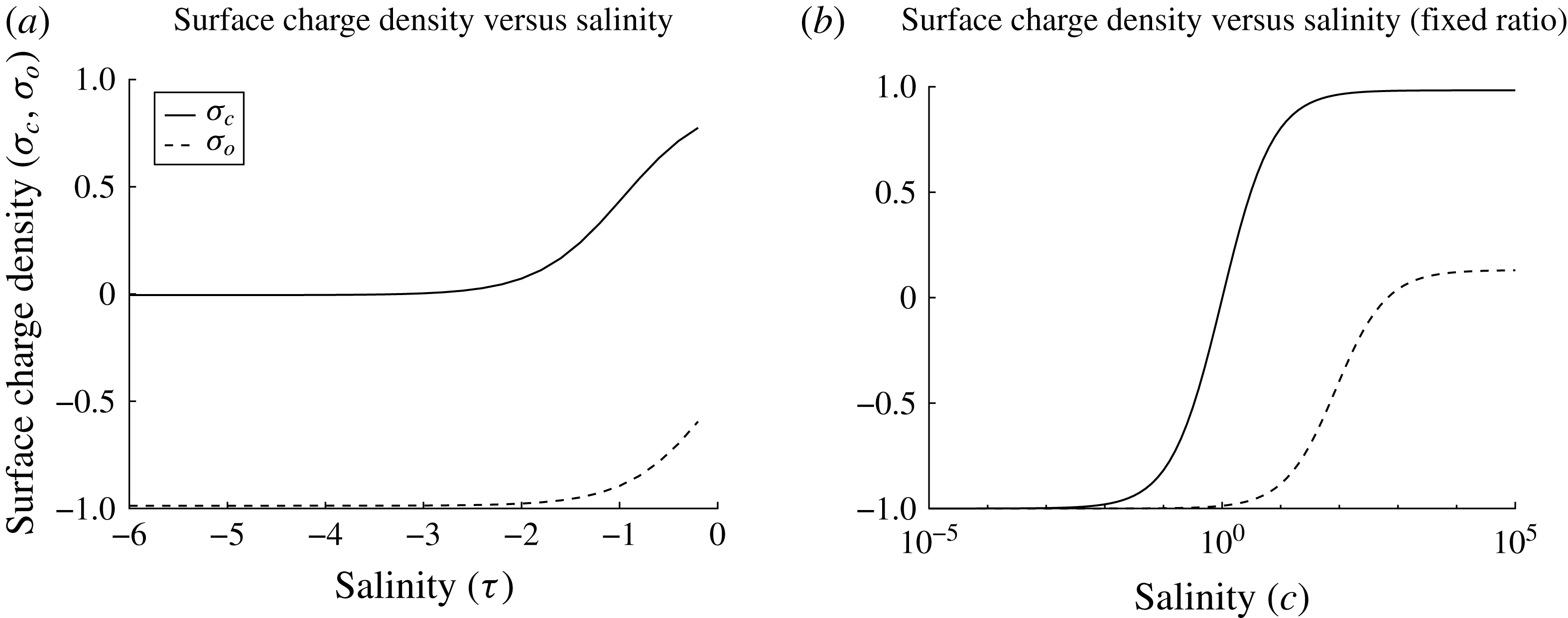
 $\unicode[STIX]{x1D70E}_{c}=q(2s_{c}^{+}+s_{c}-s_{c}^{\ast })$
and
 $\unicode[STIX]{x1D70E}_{o}=q(2s_{o}^{+}+s_{o}-s_{o}^{\ast })$
, for the clay and oil surfaces, respectively.
Owing to the charged surfaces, there is a discontinuity in the electric field across the clay–water and oil–water interfaces. We impose that the electric field is zero at infinity, since we assume that the system is globally neutral. These conditions read
 $$\begin{eqnarray}\displaystyle [\unicode[STIX]{x1D700}\unicode[STIX]{x1D719}_{z}]_{z=0^{-}}^{z=0^{+}}=\unicode[STIX]{x1D70E}_{c},\quad [\unicode[STIX]{x1D700}\boldsymbol{n}\boldsymbol{\cdot }\unicode[STIX]{x1D735}\unicode[STIX]{x1D719}]_{z=h^{-}}^{z=h^{+}}=\unicode[STIX]{x1D70E}_{o}, & & \displaystyle\end{eqnarray}$$
 $$\begin{eqnarray}\displaystyle \unicode[STIX]{x1D735}\unicode[STIX]{x1D719}\rightarrow 0,\quad \text{as }x^{2}+z^{2}\rightarrow \infty , & & \displaystyle\end{eqnarray}$$
where the permittivity is given by
 $\unicode[STIX]{x1D700}=\unicode[STIX]{x1D700}_{w}$
in the water phase,
 $\unicode[STIX]{x1D700}=\unicode[STIX]{x1D700}_{o}$
in the oil phase and
 $\unicode[STIX]{x1D700}=\unicode[STIX]{x1D700}_{c}$
in the clay phase.
Finally, we also assume that the electric potential is continuous across these interfaces,
 $$\begin{eqnarray}\displaystyle [\unicode[STIX]{x1D719}]_{z=0^{-}}^{z=0^{+}}=[\unicode[STIX]{x1D719}]_{z=h^{-}}^{z=h^{+}}=0. & & \displaystyle\end{eqnarray}$$
2.2.1 Capturing salinity variations
In order to study the effect of varying the concentrations of monovalent and divalent ions simultaneously, since this is typical for water-flood experiments, we introduce the parameter
 $\unicode[STIX]{x1D70F}$
such that
 $$\begin{eqnarray}\displaystyle c_{\infty }^{1,2}=c_{low}^{1,2}+10^{\unicode[STIX]{x1D70F}}(c_{high}^{1,2}-c_{low}^{1,2}), & & \displaystyle\end{eqnarray}$$
where
 $c_{low}^{1,2}$
are the concentrations of monovalent and divalent ions, respectively, in the low-salinity regime, and
 $c_{high}^{1,2}$
are the concentrations of monovalent and divalent ions, respectively, in the high-salinity regime. By varying
 $\unicode[STIX]{x1D70F}$
from
 $-\infty$
to 0, we can study the model continuously between the low-salinity and high-salinity regimes using a single parameter. We choose a power law for
 $\unicode[STIX]{x1D70F}$
, as typically the salinities span multiple orders of magnitude.
2.3 Non-dimensionalisation
We non-dimensionalise the problem using the following scalings:
 $$\begin{eqnarray}\displaystyle \left.\begin{array}{@{}c@{}}x=L\hat{x},\quad z=R\hat{z},\quad h=R{\hat{h}},\\ u_{w}=U\hat{u} _{w},\quad u_{o}=U\hat{u} _{o},\quad w_{w}=\unicode[STIX]{x1D716}_{1}U{\hat{w}}_{w},\quad w_{o}=\unicode[STIX]{x1D716}_{1}U{\hat{w}}_{o},\\ p_{w}=P\hat{p_{w}},\quad p_{o}=P\hat{p_{o}},\quad \displaystyle t=\frac{L}{U}\hat{t},\\ c^{\pm }=c_{low}^{1}{\hat{c}}^{\pm },\quad c^{2\pm }=c_{low}^{2}{\hat{c}}^{2\pm },\quad \displaystyle \unicode[STIX]{x1D719}=\frac{k_{B}T}{q}\hat{\unicode[STIX]{x1D719}},\quad \unicode[STIX]{x1D700}=\unicode[STIX]{x1D700}_{w}\hat{\unicode[STIX]{x1D700}},\\ s_{c}=s_{c}^{\ast }{\hat{s}}_{c},\quad s_{c}^{+}=s_{c}^{\ast }{\hat{s}}_{c}^{+},\quad s_{o}=s_{o}^{\ast }{\hat{s}}_{o},\quad s_{o}^{+}=s_{o}^{\ast }{\hat{s}}_{o}^{+}.\end{array}\right\} & & \displaystyle\end{eqnarray}$$
We choose
 $U=(PR^{2})/(\unicode[STIX]{x1D707}_{w}L)$
in order to get a balance in (2.2), and
 $\unicode[STIX]{x1D716}_{1}=R/L$
is the aspect ratio of the capillary tube. After substituting in these variables, and dropping the hats, the dimensionless equations read as follows:
 $$\begin{eqnarray}\displaystyle & \displaystyle \unicode[STIX]{x1D716}_{1}^{2}Re\frac{\text{D}u_{w}}{\text{D}t}=-{p_{w}}_{x}+(\unicode[STIX]{x1D716}_{1}^{2}{u_{w}}_{xx}+{u_{w}}_{zz})-\frac{\unicode[STIX]{x1D709}}{\unicode[STIX]{x1D6FF}P^{\ast }}(c^{+}-c^{-}+2c^{\ast }c^{2+}-2c^{\ast }c^{2-})\unicode[STIX]{x1D719}_{x},\quad \text{in }\unicode[STIX]{x1D6FA}_{w}, & \displaystyle \nonumber\\ \displaystyle & & \displaystyle\end{eqnarray}$$
 $$\begin{eqnarray}\displaystyle \unicode[STIX]{x1D716}_{1}^{4}Re\frac{\text{D}w_{w}}{\text{D}t} & = & \displaystyle -{p_{w}}_{z}+\unicode[STIX]{x1D716}_{1}^{2}(\unicode[STIX]{x1D716}_{1}^{2}{w_{w}}_{xx}+{w_{w}}_{zz})\nonumber\\ \displaystyle & & \displaystyle -\,\frac{\unicode[STIX]{x1D709}}{\unicode[STIX]{x1D6FF}P^{\ast }}(c^{+}-c^{-}+2c^{\ast }c^{2+}-2c^{\ast }c^{2-})\unicode[STIX]{x1D719}_{z},\quad \text{in }\unicode[STIX]{x1D6FA}_{w},\end{eqnarray}$$
 $$\begin{eqnarray}\displaystyle & \displaystyle {u_{w}}_{x}+{w_{w}}_{z}=0,\quad \text{in }\unicode[STIX]{x1D6FA}_{w}, & \displaystyle\end{eqnarray}$$
 $$\begin{eqnarray}\displaystyle & \displaystyle \unicode[STIX]{x1D716}_{1}^{2}\unicode[STIX]{x1D70C}^{\ast }Re\frac{\text{D}u_{o}}{\text{D}t}=-{p_{o}}_{x}+\unicode[STIX]{x1D707}^{\ast }(\unicode[STIX]{x1D716}_{1}^{2}{u_{o}}_{xx}+{u_{o}}_{zz}),\quad \text{in }\unicode[STIX]{x1D6FA}_{o}, & \displaystyle\end{eqnarray}$$
 $$\begin{eqnarray}\displaystyle & \displaystyle \unicode[STIX]{x1D716}_{1}^{4}\unicode[STIX]{x1D70C}^{\ast }Re\frac{\text{D}w_{o}}{\text{D}t}=-{p_{o}}_{z}+\unicode[STIX]{x1D716}_{1}^{2}\unicode[STIX]{x1D707}^{\ast }(\unicode[STIX]{x1D716}_{1}^{2}{w_{o}}_{xx}+{w_{o}}_{zz}),\quad \text{in }\unicode[STIX]{x1D6FA}_{o}, & \displaystyle\end{eqnarray}$$
 $$\begin{eqnarray}\displaystyle & \displaystyle {u_{o}}_{x}+{w_{o}}_{z}=0,\quad \text{in }\unicode[STIX]{x1D6FA}_{o}, & \displaystyle\end{eqnarray}$$
 $$\begin{eqnarray}\displaystyle & \displaystyle \unicode[STIX]{x1D716}_{1}^{2}Pe^{\pm }\frac{\text{D}c^{\pm }}{\text{D}t}=\unicode[STIX]{x1D716}_{1}^{2}(c_{x}^{\pm }\pm c^{\pm }\unicode[STIX]{x1D719}_{x})_{x}+(c_{z}^{\pm }\pm c^{\pm }\unicode[STIX]{x1D719}_{z})_{z},\quad \text{in }\unicode[STIX]{x1D6FA}_{w}, & \displaystyle\end{eqnarray}$$
 $$\begin{eqnarray}\displaystyle & \displaystyle \unicode[STIX]{x1D716}_{1}^{2}Pe^{2\pm }\frac{\text{D}c^{2\pm }}{\text{D}t}=\unicode[STIX]{x1D716}_{1}^{2}(c_{x}^{2\pm }\pm 2c^{2\pm }\unicode[STIX]{x1D719}_{x})_{x}+(c_{z}^{2\pm }\pm 2c^{2\pm }\unicode[STIX]{x1D719}_{z})_{z},\quad \text{in }\unicode[STIX]{x1D6FA}_{w}, & \displaystyle\end{eqnarray}$$
 $$\begin{eqnarray}\displaystyle & \displaystyle \unicode[STIX]{x1D6FF}\unicode[STIX]{x1D709}(\unicode[STIX]{x1D716}_{1}^{2}\unicode[STIX]{x1D719}_{xx}+\unicode[STIX]{x1D719}_{zz})=-(c^{+}-c^{-}+2c^{\ast }c^{2+}-2c^{\ast }c^{2-}),\quad \text{in }\unicode[STIX]{x1D6FA}_{w}, & \displaystyle\end{eqnarray}$$
 $$\begin{eqnarray}\displaystyle & \displaystyle \unicode[STIX]{x1D716}_{1}^{2}\unicode[STIX]{x1D719}_{xx}+\unicode[STIX]{x1D719}_{zz}=0,\quad \text{in }\unicode[STIX]{x1D6FA}_{o}\cup \unicode[STIX]{x1D6FA}_{c}, & \displaystyle\end{eqnarray}$$
 $$\begin{eqnarray}\displaystyle \unicode[STIX]{x1D700}=1\quad \text{in }\unicode[STIX]{x1D6FA}_{w},\quad \unicode[STIX]{x1D700}=\unicode[STIX]{x1D700}_{1}\quad \text{in }\unicode[STIX]{x1D6FA}_{o},\quad \unicode[STIX]{x1D700}=\unicode[STIX]{x1D700}_{2}\quad \text{in }\unicode[STIX]{x1D6FA}_{c}. & & \displaystyle\end{eqnarray}$$
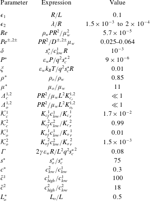
The dimensionless parameters, summarised in table 1, are as follows:
 $Re=\unicode[STIX]{x1D70C}_{w}PR^{2}/\unicode[STIX]{x1D707}_{w}^{2}$
is the Reynolds number,
 $Pe^{\pm ,2\pm }=PR^{2}/D^{\pm ,2\pm }\unicode[STIX]{x1D707}_{w}$
are the Péclet numbers for the different ionic species,
 $\unicode[STIX]{x1D6FF}=s_{c}^{\ast }/c_{low}^{1}R$
is the ratio of the adsorption depth to the radius of the capillary,
 $P^{\ast }=\unicode[STIX]{x1D700}_{w}P/q^{2}{s_{c}^{\ast }}^{2}$
is the ratio of the pressure drop across the capillary to the electrostatic pressure due to the charged surfaces,
 $\unicode[STIX]{x1D709}=\unicode[STIX]{x1D700}_{w}k_{B}T/q^{2}s_{c}^{\ast }R$
is the ratio of the thermal voltage to the potential due to the charged surfaces,
 $\unicode[STIX]{x1D70C}^{\ast }=\unicode[STIX]{x1D70C}_{o}/\unicode[STIX]{x1D70C}_{w}$
is the ratio of the density of the oil to the density of the water,
 $\unicode[STIX]{x1D707}^{\ast }=\unicode[STIX]{x1D707}_{o}/\unicode[STIX]{x1D707}_{w}$
is the ratio of the viscosity of the oil to the viscosity of the water, and
 $c^{\ast }=c_{low}^{2}/c_{low}^{1}$
is the ratio of the bulk concentration of divalent ions to the bulk concentration of monovalent ions in the low-salinity regime. The dimensionless permittivity is
 $\unicode[STIX]{x1D700}_{1}=\unicode[STIX]{x1D700}_{o}/\unicode[STIX]{x1D700}_{w}$
in the oil phase, and
 $\unicode[STIX]{x1D700}_{2}=\unicode[STIX]{x1D700}_{c}/\unicode[STIX]{x1D700}_{w}$
in the clay phase.

Equations (2.32)–(2.42) are subject to the axial boundary conditions
 $$\begin{eqnarray}\displaystyle p_{w}=1,\quad c^{\pm ,2\pm }=1+10^{\unicode[STIX]{x1D70F}}(\bar{c}^{1,2}-1),\quad \text{at }x=0, & & \displaystyle\end{eqnarray}$$
 $$\begin{eqnarray}\displaystyle p_{w}=0,\quad c^{\pm ,2\pm }=1+10^{\unicode[STIX]{x1D70F}}(\bar{c}^{1,2}-1),\quad \text{at }x=1, & & \displaystyle\end{eqnarray}$$
as well as the zero net current constraint
 $$\begin{eqnarray}\displaystyle \int _{0}^{1}\left\{\frac{c_{x}^{+}+c^{+}\unicode[STIX]{x1D719}_{x}}{Pe^{+}}-\frac{c_{x}^{-}-c^{-}\unicode[STIX]{x1D719}_{x}}{Pe^{-}}+2c^{\ast }\left[\frac{c_{x}^{2+}+2c^{2+}\unicode[STIX]{x1D719}_{x}}{Pe^{2+}}-\frac{c_{x}^{2-}-2c^{2-}\unicode[STIX]{x1D719}_{x}}{Pe^{2-}}\right]\right\}\text{d}z=0, & & \displaystyle\end{eqnarray}$$
at
 $x=0$
, where we have substituted (2.6) and (2.7). We also have that
 $$\begin{eqnarray}\displaystyle \left.\begin{array}{@{}c@{}}\boldsymbol{u}_{w}=0,\quad \unicode[STIX]{x1D709}[\unicode[STIX]{x1D700}\unicode[STIX]{x1D719}_{z}]_{z=0^{-}}^{z=0^{+}}=2s_{c}^{+}+s_{c}-1,\quad [\unicode[STIX]{x1D719}]_{z=0^{-}}^{z=0^{+}}=0,\\ \displaystyle \unicode[STIX]{x1D6EC}_{c}^{1}\frac{\unicode[STIX]{x2202}s_{c}}{\unicode[STIX]{x2202}t}={\mathcal{K}}_{c}^{1}c^{+}(1-s_{c}-s_{c}^{+})-s_{c},\\ \displaystyle \unicode[STIX]{x1D6EC}_{c}^{2}\frac{\unicode[STIX]{x2202}s_{c}^{+}}{\unicode[STIX]{x2202}t}={\mathcal{K}}_{c}^{2}c^{2+}(1-s_{c}-s_{c}^{+})-s_{c}^{+},\\ \displaystyle c_{z}^{+}+c^{+}\unicode[STIX]{x1D719}_{z}=\unicode[STIX]{x1D716}_{1}^{2}\unicode[STIX]{x1D6FF}\,Pe^{+}\frac{\unicode[STIX]{x2202}s_{c}}{\unicode[STIX]{x2202}t},\quad c_{z}^{-}-c^{-}\unicode[STIX]{x1D719}_{z}=0,\\ \displaystyle c_{z}^{2+}+2c^{2+}\unicode[STIX]{x1D719}_{z}=\frac{\unicode[STIX]{x1D716}_{1}^{2}\unicode[STIX]{x1D6FF}\,Pe^{2+}}{c^{\ast }}\frac{\unicode[STIX]{x2202}s_{c}^{+}}{\unicode[STIX]{x2202}t},\quad c_{z}^{2-}-2c^{2-}\unicode[STIX]{x1D719}_{z}=0,\end{array}\right\}\quad z & =0, & \displaystyle\end{eqnarray}$$
 $$\begin{eqnarray}\left.\begin{array}{@{}c@{}}\boldsymbol{u}_{w}=\boldsymbol{u}_{o},\quad h_{t}=w_{w}-u_{w}h_{x},\quad [\unicode[STIX]{x1D719}]_{z=h^{-}}^{z=h^{+}}=0,\\ \displaystyle \frac{\unicode[STIX]{x1D709}}{(1+\unicode[STIX]{x1D716}_{1}^{2}h_{x}^{2})^{1/2}}[\unicode[STIX]{x1D700}(\unicode[STIX]{x1D719}_{z}-\unicode[STIX]{x1D716}_{1}^{2}h_{x}\unicode[STIX]{x1D719}_{x})]_{z=h^{-}}^{z=h^{+}}=s^{\ast }(2s_{o}^{+}+s_{o}-1),\\ \displaystyle \unicode[STIX]{x1D6EC}_{o}^{1}\frac{\text{D}s_{o}}{\text{D}t}={\mathcal{K}}_{o}^{1}c^{+}(1-s_{o}-s_{o}^{+})-s_{o},\\ \displaystyle \unicode[STIX]{x1D6EC}_{o}^{2}\frac{\text{D}s_{o}^{+}}{\text{D}t}={\mathcal{K}}_{o}^{2}c^{2+}(1-s_{o}-s_{o}^{+})-s_{o}^{+},\\ \displaystyle c_{z}^{+}+c^{+}\unicode[STIX]{x1D719}_{z}-\unicode[STIX]{x1D716}_{1}^{2}h_{x}(c_{x}^{+}+c^{+}\unicode[STIX]{x1D719}_{x})=\unicode[STIX]{x1D716}_{1}^{2}\,Pe^{+}\left(h_{x}u_{w}c^{+}-w_{w}c^{+}-\unicode[STIX]{x1D6FF}s^{\ast }\frac{\text{D}s_{o}}{\text{D}t}\right),\\ \displaystyle c_{z}^{2+}+2c^{2+}\unicode[STIX]{x1D719}_{z}-\unicode[STIX]{x1D716}_{1}^{2}h_{x}(c_{x}^{2+}+2c^{2+}\unicode[STIX]{x1D719}_{x})=\unicode[STIX]{x1D716}_{1}^{2}\,Pe^{2+}\left(h_{x}u_{w}c^{2+}-w_{w}c^{2+}-\frac{\unicode[STIX]{x1D6FF}s^{\ast }}{c^{\ast }}\frac{\text{D}s_{o}^{+}}{\text{D}t}\right),\\ c_{z}^{-}-c^{-}\unicode[STIX]{x1D719}_{z}-\unicode[STIX]{x1D716}_{1}^{2}h_{x}(c_{x}^{-}-c^{-}\unicode[STIX]{x1D719}_{x})=\unicode[STIX]{x1D716}_{1}^{2}\,Pe^{-}(h_{x}u_{w}c^{-}-w_{w}c^{-}),\\ c_{z}^{2-}-2c^{2-}\unicode[STIX]{x1D719}_{z}-\unicode[STIX]{x1D716}_{1}^{2}h_{x}(c_{x}^{2-}-2c^{2-}\unicode[STIX]{x1D719}_{x})=\unicode[STIX]{x1D716}_{1}^{2}\,Pe^{2-}(h_{x}u_{w}c^{2-}-w_{w}c^{2-}),\end{array}\right\}\quad z=h,\end{eqnarray}$$
 $$\begin{eqnarray}\displaystyle & & \displaystyle \unicode[STIX]{x1D707}^{\ast }[({u_{o}}_{z}+\unicode[STIX]{x1D716}_{1}{w_{o}}_{z})(1-\unicode[STIX]{x1D716}_{1}^{2}h_{x}^{2})+2\unicode[STIX]{x1D716}_{1}^{2}h_{x}({w_{o}}_{z}-{u_{o}}_{x})]=({u_{w}}_{z}+\unicode[STIX]{x1D716}_{1}{w_{w}}_{z})(1-\unicode[STIX]{x1D716}_{1}^{2}h_{x}^{2})\nonumber\\ \displaystyle & & \displaystyle \quad +\,2\unicode[STIX]{x1D716}_{1}^{2}h_{x}({w_{w}}_{z}-{u_{w}}_{x})-\frac{\unicode[STIX]{x1D716}_{1}}{P^{\ast }}[h_{x}(\unicode[STIX]{x1D716}_{1}^{2}\unicode[STIX]{x1D719}_{x}^{2}-\unicode[STIX]{x1D719}_{z}^{2})+(1-\unicode[STIX]{x1D716}_{1}^{2}h_{x}^{2})\unicode[STIX]{x1D719}_{x}\unicode[STIX]{x1D719}_{z}]_{z=h^{-}}^{z=h^{+}},\quad \text{on }z=h,\end{eqnarray}$$
 $$\begin{eqnarray}\displaystyle & & \displaystyle \unicode[STIX]{x1D716}_{1}^{2}\unicode[STIX]{x1D707}^{\ast }\frac{[{w_{o}}_{z}-h_{x}{u_{o}}_{z}+\unicode[STIX]{x1D716}_{1}^{2}h_{x}(h_{x}{u_{o}}_{x}-{w_{o}}_{x})]}{1+\unicode[STIX]{x1D716}_{1}^{2}h_{x}^{2}}=\unicode[STIX]{x1D716}_{1}^{2}\frac{[{w_{w}}_{z}-h_{x}{u_{w}}_{z}+\unicode[STIX]{x1D716}_{1}^{2}h_{x}(h_{x}{u_{w}}_{x}-{w_{w}}_{x})]}{1+\unicode[STIX]{x1D716}_{1}^{2}h_{x}^{2}}\nonumber\\ \displaystyle & & \displaystyle \quad +\,\frac{1}{2}(p_{o}-p_{w})+\frac{\unicode[STIX]{x1D709}^{2}}{P^{\ast }}\left[\frac{\unicode[STIX]{x1D716}_{1}^{2}h_{x}\unicode[STIX]{x1D719}_{x}\unicode[STIX]{x1D719}_{z}}{1+\unicode[STIX]{x1D716}_{1}^{2}h_{x}^{2}}+\frac{1}{4}(\unicode[STIX]{x1D716}_{1}^{2}\unicode[STIX]{x1D719}_{x}^{2}-\unicode[STIX]{x1D719}_{z}^{2})\right]_{z=h^{-}}^{z=h^{+}}\nonumber\\ \displaystyle & & \displaystyle \quad -\,\frac{\unicode[STIX]{x1D6E4}h_{xx}}{4P^{\ast }(1+\unicode[STIX]{x1D716}_{1}^{2}h_{x}^{2})^{3/2}},\quad \text{on }z=h,\end{eqnarray}$$
 $$\begin{eqnarray}\displaystyle & \displaystyle {u_{w}}_{z}={u_{o}}_{z}=w_{w}=w_{o}={p_{w}}_{z}={p_{o}}_{z}=c_{z}^{\pm }=c_{z}^{2\pm }=\unicode[STIX]{x1D719}_{z}=0,\quad \text{at }z=1, & \displaystyle\end{eqnarray}$$
 $$\begin{eqnarray}\displaystyle & \displaystyle \unicode[STIX]{x1D735}\unicode[STIX]{x1D719}\rightarrow \mathbf{0},\quad \text{as }x^{2}+z^{2}\rightarrow \infty , & \displaystyle\end{eqnarray}$$
where we have substituted in the expressions for the stress tensors, equations (2.19) and (2.20), into the boundary conditions on the oil–water interface, equations (2.17) and (2.18), to obtain (2.48) and (2.49).
The ratios of the ion concentrations in the high-salinity and low-salinity regimes are given by
 $\bar{c}^{1,2}=c_{high}^{1,2}/c_{low}^{1,2}$
, the ratios of the time scales of the surface reactions to the flow time scale are given by
 $\unicode[STIX]{x1D6EC}_{c}^{1,2}=PR^{2}/\unicode[STIX]{x1D707}_{w}L^{2}K_{c_{r}}^{1,2}$
and
 $\unicode[STIX]{x1D6EC}_{o}^{1,2}=PR^{2}/\unicode[STIX]{x1D707}_{w}L^{2}K_{o_{r}}^{1,2}$
, the dimensionless equilibrium constants are
 ${\mathcal{K}}_{c}^{1,2}={K_{c}}_{f}^{1,2}c_{low}^{1,2}/{K_{c}}_{r}^{1,2}$
and
 ${\mathcal{K}}_{o}^{1,2}={K_{o}}_{f}^{1,2}c_{low}^{1,2}/{K_{o}}_{r}^{1,2}$
, the ratio of the surface tension forces to the electrostatic forces is
 $\unicode[STIX]{x1D6E4}=2\unicode[STIX]{x1D6FE}\unicode[STIX]{x1D700}_{w}R/L^{2}q^{2}{s_{c}^{\ast }}^{2}$
(we note that
 $2\unicode[STIX]{x1D716}_{1}^{3}P^{\ast }/\unicode[STIX]{x1D6E4}$
is the capillary number), and
 $s^{\ast }=s_{o}^{\ast }/s_{c}^{\ast }$
is the ratio of the saturation concentration of the oil surface to the saturation concentration of the clay surface.
Austad et al. (Reference Austad, Rezaeidoust and Puntervold2010) performed experiments using brine with low salinity concentrations
 $c_{low}^{1}\approx 17~\text{mol}~\text{m}^{-3}$
,
 $c_{low}^{2}\approx 5~\text{mol}~\text{m}^{-3}$
, and high salinity concentrations
 $c_{high}^{1}\approx 1.7\times 10^{3}~\text{mol}~\text{m}^{-3}$
,
 $c_{high}^{2}\approx 90~\text{mol}~\text{m}^{-3}$
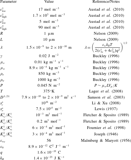
; hence we take these to be our low-salinity and high-salinity regimes, respectively. In a given sample of reservoir rock, there will be a range of pore throat sizes. Nelson (Reference Nelson2009) studied the distribution of these throat sizes for various rocks, and for the purposes of this paper we assume
 $R=1~\unicode[STIX]{x03BC}\text{m}$
, which is typical for a sandstone reservoir. The grain size, and hence the length of a typical pore throat, is typically an order of magnitude larger, so we assume that
 $L=10~\unicode[STIX]{x03BC}\text{m}$
. For the oil viscosity, density and interfacial tension, we use values determined by Buckley (Reference Buckley1996) for a range of oil samples. Typically,
 $\unicode[STIX]{x1D6FE}\approx 0.02~\text{N}~\text{m}^{-1}$
, with some variation depending on the pH. The viscosities of the oils used by Buckley ranged from
 $0.006$
to
 $0.035~\text{kg}~\text{m}^{-1}~\text{s}^{-1}$
, so we choose
 $\unicode[STIX]{x1D707}_{o}=0.01~\text{kg}~\text{m}^{-1}~\text{s}^{-1}$
. The oil densities were in the range
 $840{-}900~\text{kg}~\text{m}^{-3}$
, so we choose
 $\unicode[STIX]{x1D70C}_{o}=850~\text{kg}~\text{m}^{-3}$
. The viscosity of water is
 $8.9\times 10^{-4}~\text{kg}~\text{m}^{-1}~\text{s}^{-1}$
, and the density of water is in the range
 $1000~\text{kg}~\text{m}^{-3}$
(pure water) to
 $1027~\text{kg}~\text{m}^{-3}$
(seawater), so we choose
 $\unicode[STIX]{x1D70C}_{w}=1000~\text{kg}~\text{m}^{-3}$
for simplicity. Injection rates used in core experiments vary considerably (Jadhunandan Reference Jadhunandan1990). For the purposes of this paper, we assume that the flow velocity within the pores of a reservoir is
 $V_{p}=1.5\times 10^{-5}~\text{m}~\text{s}^{-1}$
(
 ${\approx}4~\text{ft}~\text{day}^{-1}$
). We estimate the pressure using Darcy’s law,
 $\unicode[STIX]{x1D713}V_{p}=KP/\unicode[STIX]{x1D707}L$
, where
 $K$
is the permeability of the reservoir rock, and
 $\unicode[STIX]{x1D713}$
is the porosity. For
 $K/\unicode[STIX]{x1D713}=3000~\text{mD}$
(Ligthelm et al.
Reference Ligthelm, Gronsveld, Hofman, Brussee, Marcelis and van der Linde2009), this gives
 $P\approx 0.045~\text{N}~\text{m}^{-2}$
.
Lager et al. (Reference Lager, Webb, Black, Singleton and Sorbie2008) performed core-scale experiments at
 $102\,^{\circ }\text{C}$
, so we choose
 $T=375~\text{K}$
. Using
 $\unicode[STIX]{x1D700}_{w}={\unicode[STIX]{x1D700}_{w}}_{r}\unicode[STIX]{x1D700}_{0}$
, where
 ${\unicode[STIX]{x1D700}_{w}}_{r}\approx 56$
(Malmberg & Maryott Reference Malmberg and Maryott1956) and
 $\unicode[STIX]{x1D700}_{0}\approx 8.9\times 10^{-12}~\text{C}^{2}~\text{J}^{-1}~\text{m}^{-1}$
are the relative permittivity of water at
 $100\,^{\circ }\text{C}$
and the permittivity of free space, respectively, we find that
 $\unicode[STIX]{x1D700}_{w}\approx 5\times 10^{-10}~\text{C}^{2}~\text{J}^{-1}~\text{m}^{-1}$
. We take
 $D^{+}\approx 1.3\times 10^{-9}~\text{m}^{2}~\text{s}^{-1}$
,
 $D^{-}\approx 2\times 10^{-9}~\text{m}^{2}~\text{s}^{-1}$
,
 $D^{2+}\approx 7.9\times 10^{-10}~\text{m}^{2}~\text{s}^{-1}$
and
 $D^{2-}\approx 1.1\times 10^{-9}~\text{m}^{2}~\text{s}^{-1}$
, as these are the mass diffusivities of sodium, chloride, sulfate and calcium ions, respectively (Samson, Marchand & Snyder Reference Samson, Marchand and Snyder2003). We use the standard values for
 $q\approx 1.6\times 10^{-19}~\text{C}$
and
 $k_{B}\approx 1.4\times 10^{-23}~\text{J}~\text{K}^{-1}$
.
Fletcher & Sposito (Reference Fletcher and Sposito1989) study the equilibrium constants for a sample of montmorillonite. From these results, we estimate that
 $K_{c_{f}}^{1}/K_{c_{r}}^{1}=10^{-3}~\text{m}^{3}~\text{mol}^{-1}$
and
 $K_{c_{f}}^{2}/K_{c_{r}}^{2}=0.2~\text{m}^{3}~\text{mol}^{-1}$
. The ion exchange reactions occurring in the MIE mechanism involve the dissociation and recombination of monovalent and divalent cations with carboxylic acid groups on the oil surface. We assume that the monovalent and divalent cations are sodium and calcium, respectively, and that the carboxylic acid on the oil surface is acetic acid. The
 $\text{p}K_{a}$
values of sodium acetate and calcium acetate are approximately
 $-0.2$
(Fournier et al.
Reference Fournier, Oelkers, Gout and Pokrovski1998) and
 $-0.53$
(Joseph Reference Joseph1946), respectively, so we take the equilibrium constants for the reactions occurring on the oil surface to be
 $K_{o_{f}}^{1}/K_{o_{r}}^{1}\approx 6\times 10^{-4}~\text{m}^{3}~\text{mol}^{-1}$
and
 $K_{o_{f}}^{2}/K_{o_{r}}^{2}\approx 3\times 10^{-4}~\text{m}^{3}~\text{mol}^{-1}$
. Li & Xu (Reference Li and Xu2008) studied the surface charge densities for different clays for various values of the pH of the surrounding fluid. For a binary system containing kaolinite, a typical maximum surface charge is approximately
 $\unicode[STIX]{x1D70E}_{c}^{max}=5\times 10^{-4}~\text{C}~\text{m}^{-2}$
. Hence, by supposing that
 $\unicode[STIX]{x1D70E}_{c}^{max}\approx qs_{c}^{\ast }$
, we estimate that
 $s_{c}^{\ast }\approx 10^{16}~\text{m}^{-2}$
. Lewis (Reference Lewis1937) studied the maximum charge at an oil–water interface, from which we estimate that the saturation concentration is approximately
 $s_{o}^{\ast }\approx 7.5\times 10^{17}~\text{m}^{-2}$
. We present a summary of the dimensional parameters in the model in table 2.
Dimensional parameters.
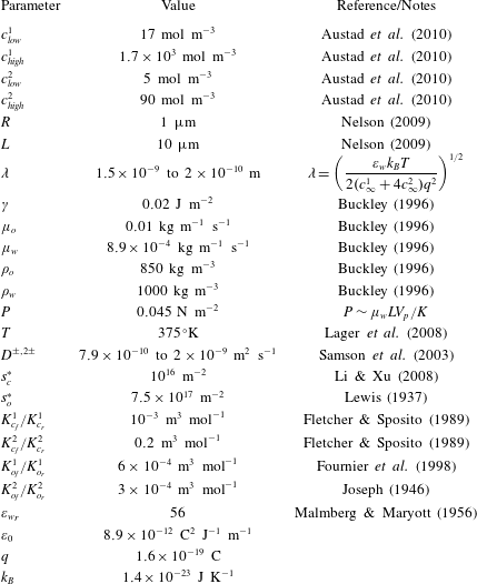
Using these values, we find that
 $\unicode[STIX]{x1D716}_{1}\approx 0.1\ll 1$
. The Reynolds number is
 $Re\approx 5.7\times 10^{-5}\ll 1$
, and therefore we neglect the inertial terms in the Navier–Stokes equations. The Péclet numbers are
 $Pe^{+}\approx 0.039$
,
 $Pe^{-}\approx 0.025$
,
 $Pe^{2+}\approx 0.064$
and
 $Pe^{2-}\approx 0.046$
; we will assume that these are all
 $O(1)$
for generality. We also assume that the ions react quickly at the surfaces by comparison to the flow time scale so that instantaneous adsorption occurs, that is, we assume that
 $\unicode[STIX]{x1D6EC}_{c}^{1,2}\ll 1$
and
 $\unicode[STIX]{x1D6EC}_{o}^{1,2}\ll 1$
.
We find that the ratio of the adsorption depth to the capillary radius is given by
 $\unicode[STIX]{x1D709}\approx 0.01$
and the ratio of the thermal voltage to the potential due to charged surfaces is
 $\unicode[STIX]{x1D6FF}\approx 10^{-3}$
. Thus we suppose that
 $\unicode[STIX]{x1D6FF}\ll \unicode[STIX]{x1D709}\ll 1$
. We find that
 $\unicode[STIX]{x1D6E4}\approx 0.08$
, which we take to be
 $O(1)$
for generality, and
 $P^{\ast }\approx 9\times 10^{-6}$
. We will find later that viscous effects become important for
 $P^{\ast }\approx 10^{-5}$
, hence we will not neglect terms proportional to
 $P^{\ast }$
at this stage. In § 4.5 we will consider the limit
 $P^{\ast }\rightarrow 0$
. The values of the dimensionless parameters in the model are presented in table 1.
Neglecting terms proportional to
 $\unicode[STIX]{x1D716}_{1}$
,
 $Re$
,
 $\unicode[STIX]{x1D6EC}_{c}^{1,2}$
and
 $\unicode[STIX]{x1D6EC}_{o}^{1,2}$
, equations (2.32)–(2.51) read
 $$\begin{eqnarray}\displaystyle & \left.\begin{array}{@{}c@{}}\displaystyle {u_{w}}_{zz}={p_{w}}_{x}+\frac{\unicode[STIX]{x1D709}}{\unicode[STIX]{x1D6FF}P^{\ast }}(c^{+}-c^{-}+2c^{\ast }c^{2+}-2c^{\ast }c^{2-})\unicode[STIX]{x1D719}_{x},\\ \displaystyle {p_{w}}_{z}=\frac{\unicode[STIX]{x1D709}}{\unicode[STIX]{x1D6FF}P^{\ast }}(c^{+}-c^{-}+2c^{\ast }c^{2+}-2c^{\ast }c^{2-})\unicode[STIX]{x1D719}_{z},\\ {u_{w}}_{x}+{w_{w}}_{z}=0,\end{array}\right\}\quad \text{in }\unicode[STIX]{x1D6FA}_{w}, & \displaystyle\end{eqnarray}$$
 $$\begin{eqnarray}\displaystyle \unicode[STIX]{x1D707}^{\ast }{u_{o}}_{zz}={p_{o}}_{x},\quad {p_{o}}_{z}=0,\quad {u_{o}}_{x}+{w_{o}}_{z}=0,\quad \text{in }\unicode[STIX]{x1D6FA}_{o}, & & \displaystyle\end{eqnarray}$$
 $$\begin{eqnarray}\displaystyle (c_{z}^{\pm }\pm c^{\pm }\unicode[STIX]{x1D719}_{z})_{z}=0,\quad (c_{z}^{2\pm }\pm 2c^{2\pm }\unicode[STIX]{x1D719}_{z})_{z}=0,\quad \text{in }\unicode[STIX]{x1D6FA}_{w}, & & \displaystyle\end{eqnarray}$$
 $$\begin{eqnarray}\displaystyle \unicode[STIX]{x1D6FF}\unicode[STIX]{x1D709}\unicode[STIX]{x1D719}_{zz}=\left\{\begin{array}{@{}ll@{}}-(c^{+}-c^{-}+2c^{\ast }c^{2+}-2c^{\ast }c^{2-}),\quad & \text{in }\unicode[STIX]{x1D6FA}_{w},\\ 0,\quad & \text{in }\unicode[STIX]{x1D6FA}_{o}\cup \unicode[STIX]{x1D6FA}_{c},\end{array}\right. & & \displaystyle\end{eqnarray}$$
 $$\begin{eqnarray}\displaystyle \unicode[STIX]{x1D700}=1\quad \text{in }\unicode[STIX]{x1D6FA}_{w},\quad \unicode[STIX]{x1D700}=\unicode[STIX]{x1D700}_{1}\quad \text{in }\unicode[STIX]{x1D6FA}_{o},\quad \unicode[STIX]{x1D700}=\unicode[STIX]{x1D700}_{2}\quad \text{in }\unicode[STIX]{x1D6FA}_{c}, & & \displaystyle\end{eqnarray}$$
subject to
 $$\begin{eqnarray}\displaystyle p_{w}=1,\quad c^{\pm ,2\pm }=1+10^{\unicode[STIX]{x1D70F}}(\bar{c}^{1,2}-1),\quad x=0, & & \displaystyle\end{eqnarray}$$
 $$\begin{eqnarray}\displaystyle p_{w}=0,\quad c^{\pm ,2\pm }=1+10^{\unicode[STIX]{x1D70F}}(\bar{c}^{1,2}-1),\quad x=1, & & \displaystyle\end{eqnarray}$$
 $$\begin{eqnarray}\displaystyle & & \displaystyle \int _{0}^{1}\left\{\frac{c_{x}^{+}+c^{+}\unicode[STIX]{x1D719}_{x}}{Pe^{+}}-\frac{c_{x}^{-}-c^{-}\unicode[STIX]{x1D719}_{x}}{Pe^{-}}\right.\nonumber\\ \displaystyle & & \displaystyle \quad \left.+\,2c^{\ast }\left[\frac{c_{x}^{2+}+2c^{2+}\unicode[STIX]{x1D719}_{x}}{Pe^{2+}}-\frac{c_{x}^{2-}-2c^{2-}\unicode[STIX]{x1D719}_{x}}{Pe^{2-}}\right]\right\}\,\text{d}z=0,\quad x=0,\end{eqnarray}$$
 $$\begin{eqnarray}\displaystyle \left.\begin{array}{@{}c@{}}\boldsymbol{u}_{w}=0,\quad \unicode[STIX]{x1D709}[\unicode[STIX]{x1D700}\unicode[STIX]{x1D719}_{z}]_{z=0^{-}}^{z=0^{+}}=2s_{c}^{+}+s_{c}-1,\quad [\unicode[STIX]{x1D719}]_{z=0^{-}}^{z=0^{+}}=0,\\ {\mathcal{K}}_{c}^{1}c^{+}(1-s_{c}-s_{c}^{+})-s_{c}=0,\\ {\mathcal{K}}_{c}^{2}c^{2+}(1-s_{c}-s_{c}^{+})-s_{c}^{+}=0,\\ c_{z}^{\pm }\pm c^{\pm }\unicode[STIX]{x1D719}_{z}=0,\quad c_{z}^{2\pm }\pm 2c^{2\pm }\unicode[STIX]{x1D719}_{z}=0,\end{array}\right\}\quad z=0, & & \displaystyle\end{eqnarray}$$
 $$\begin{eqnarray}\displaystyle & \displaystyle \left.\begin{array}{@{}c@{}}\boldsymbol{u}_{w}=\boldsymbol{u}_{o},\quad \unicode[STIX]{x1D709}[\unicode[STIX]{x1D700}\unicode[STIX]{x1D719}_{z}]_{-}^{+}=s^{\ast }(2s_{o}^{+}+s_{o}-1),\quad [\unicode[STIX]{x1D719}]_{z=h^{-}}^{z=h^{+}}=0,\\ {\mathcal{K}}_{o}^{1}c^{+}(1-s_{o}-s_{o}^{+})-s_{o}=0,\\ {\mathcal{K}}_{o}^{2}c^{2+}(1-s_{o}-s_{o}^{+})-s_{o}^{+}=0,\\ c_{z}^{\pm }\pm c^{\pm }\unicode[STIX]{x1D719}_{z}=0,\quad c_{z}^{2\pm }\pm 2c^{2\pm }\unicode[STIX]{x1D719}_{z}=0,\\ h_{t}=w_{w}-u_{w}h_{x},\quad \unicode[STIX]{x1D707}^{\ast }{u_{o}}_{z}={u_{w}}_{z},\\ p_{w}=p_{o}-\displaystyle \frac{\unicode[STIX]{x1D709}^{2}}{2P^{\ast }}[\unicode[STIX]{x1D719}_{z}^{2}]_{z=h^{-}}^{z=h^{+}}-\frac{\unicode[STIX]{x1D6E4}h_{xx}}{2P^{\ast }},\end{array}\right\}\quad z=h, & \displaystyle\end{eqnarray}$$
 $$\begin{eqnarray}\displaystyle & \displaystyle {u_{w}}_{z}={u_{o}}_{z}=w_{w}=w_{o}={p_{w}}_{z}={p_{o}}_{z}=c_{z}^{\pm }=c_{z}^{2\pm }=\unicode[STIX]{x1D719}_{z}=0,\quad z=1, & \displaystyle\end{eqnarray}$$
 $$\begin{eqnarray}\displaystyle & \displaystyle \unicode[STIX]{x1D735}\unicode[STIX]{x1D719}\rightarrow \mathbf{0},\quad x^{2}+z^{2}\rightarrow \infty . & \displaystyle\end{eqnarray}$$
Taking the limit
 $\unicode[STIX]{x1D716}_{1}\rightarrow 0$
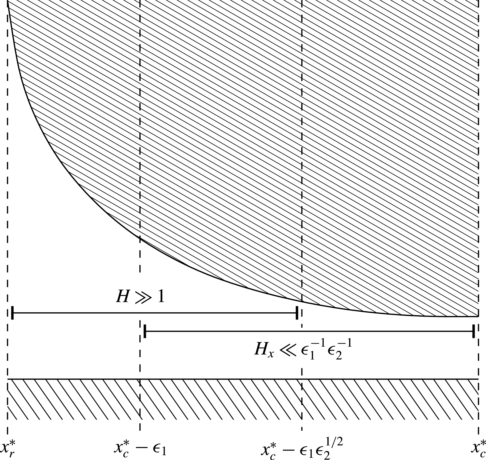
has resulted in a system that is not closed: the extra information we need arises from solvability conditions on higher-order terms in the expansion when substituted into (2.38) and (2.39). To find these conditions, we separate the water phase into five regions, as shown in figure 3: the bulk region of water to the left of the oil slug (region I); the thin layer of water separating the oil from the capillary walls (region II); the bulk region of water to the right of the oil slug (region III); and the meniscus regions at each end of the oil slug (regions IV and V). We integrate (2.38) and (2.39), and impose (2.46), (2.47) and (2.50), to get
 $$\begin{eqnarray}\displaystyle & \displaystyle Pe^{+}\int _{0}^{1}\frac{\text{D}c^{+}}{\text{D}t}\,\text{d}z=\frac{\unicode[STIX]{x2202}}{\unicode[STIX]{x2202}x}\int _{0}^{1}\left(\frac{\unicode[STIX]{x2202}c^{+}}{\unicode[STIX]{x2202}x}+c^{+}\frac{\unicode[STIX]{x2202}\unicode[STIX]{x1D719}}{\unicode[STIX]{x2202}x}\right)\text{d}z-\unicode[STIX]{x1D6FF}\,Pe^{+}\frac{\unicode[STIX]{x2202}s_{c}}{\unicode[STIX]{x2202}t}, & \displaystyle\end{eqnarray}$$
 $$\begin{eqnarray}\displaystyle & \displaystyle Pe^{2+}\int _{0}^{1}\frac{\text{D}c^{2+}}{\text{D}t}\,\text{d}z=\frac{\unicode[STIX]{x2202}}{\unicode[STIX]{x2202}x}\int _{0}^{1}\left(\frac{\unicode[STIX]{x2202}c^{2+}}{\unicode[STIX]{x2202}x}+2c^{2+}\frac{\unicode[STIX]{x2202}\unicode[STIX]{x1D719}}{\unicode[STIX]{x2202}x}\right)\text{d}z-\frac{\unicode[STIX]{x1D6FF}\,Pe^{2+}}{c^{\ast }}\frac{\unicode[STIX]{x2202}s_{c}^{+}}{\unicode[STIX]{x2202}t}, & \displaystyle\end{eqnarray}$$
 $$\begin{eqnarray}\displaystyle & \displaystyle Pe^{k-}\int _{0}^{1}\frac{\text{D}c^{k-}}{\text{D}t}\,\text{d}z=\frac{\unicode[STIX]{x2202}}{\unicode[STIX]{x2202}x}\int _{0}^{1}\left(\frac{\unicode[STIX]{x2202}c^{k-}}{\unicode[STIX]{x2202}x}-kc^{k-}\frac{\unicode[STIX]{x2202}\unicode[STIX]{x1D719}}{\unicode[STIX]{x2202}x}\right)\text{d}z,\quad \text{for }k=1,2, & \displaystyle\end{eqnarray}$$
in regions I and III, and
 $$\begin{eqnarray}\displaystyle Pe^{+}\int _{0}^{h}\frac{\text{D}c^{+}}{\text{D}t}\,\text{d}z & = & \displaystyle \frac{\unicode[STIX]{x2202}}{\unicode[STIX]{x2202}x}\int _{0}^{h}\left(\frac{\unicode[STIX]{x2202}c^{+}}{\unicode[STIX]{x2202}x}+c^{+}\frac{\unicode[STIX]{x2202}\unicode[STIX]{x1D719}}{\unicode[STIX]{x2202}x}\right)\text{d}z\nonumber\\ \displaystyle & & \displaystyle -\,\unicode[STIX]{x1D6FF}\,Pe^{+}\left(s^{\ast }\frac{\text{D}s_{o}}{\text{D}t}+\frac{\unicode[STIX]{x2202}s_{c}}{\unicode[STIX]{x2202}t}\right)-Pe^{+}\frac{\unicode[STIX]{x2202}h}{\unicode[STIX]{x2202}t}c^{+}|^{z=h},\end{eqnarray}$$
 $$\begin{eqnarray}\displaystyle Pe^{2+}\int _{0}^{h}\frac{\text{D}c^{2+}}{\text{D}t}\,\text{d}z & = & \displaystyle \frac{\unicode[STIX]{x2202}}{\unicode[STIX]{x2202}x}\int _{0}^{h}\left(\frac{\unicode[STIX]{x2202}c^{2+}}{\unicode[STIX]{x2202}x}+2c^{2+}\frac{\unicode[STIX]{x2202}\unicode[STIX]{x1D719}}{\unicode[STIX]{x2202}x}\right)\text{d}z\nonumber\\ \displaystyle & & \displaystyle -\,\frac{\unicode[STIX]{x1D6FF}\,Pe^{2+}}{c^{\ast }}\left(s^{\ast }\frac{\text{D}s_{o}^{+}}{\text{D}t}+\frac{\unicode[STIX]{x2202}s_{c}^{+}}{\unicode[STIX]{x2202}t}\right)-Pe^{2+}\frac{\unicode[STIX]{x2202}h}{\unicode[STIX]{x2202}t}c^{2+}|^{z=h},\end{eqnarray}$$
 $$\begin{eqnarray}\displaystyle Pe^{k-}\int _{0}^{h}\frac{\text{D}c^{k-}}{\text{D}t}\,\text{d}z & = & \displaystyle \frac{\unicode[STIX]{x2202}}{\unicode[STIX]{x2202}x}\int _{0}^{h}\left(\frac{\unicode[STIX]{x2202}c^{k-}}{\unicode[STIX]{x2202}x}-kc^{k-}\frac{\unicode[STIX]{x2202}\unicode[STIX]{x1D719}}{\unicode[STIX]{x2202}x}\right)\,\text{d}z-Pe^{k-}\frac{\unicode[STIX]{x2202}h}{\unicode[STIX]{x2202}t}c^{k-}|^{z=h},\end{eqnarray}$$
in regions II, IV and V for
 $k=1,2$
. Note that we have swapped the order of integration and differentiation in (2.67)–(2.69) by applying the kinematic and flux boundary conditions in (2.47). Equations (2.52)–(2.69) form a closed system of equations and boundary conditions for
 $u_{w}$
,
 $u_{o}$
,
 $w_{w}$
,
 $w_{o}$
,
 $p_{w}$
,
 $p_{o}$
,
 $c^{\pm }$
,
 $c^{2\pm }$
,
 $\unicode[STIX]{x1D719}$
,
 $s_{c}$
,
 $s_{c}^{+}$
,
 $s_{o}$
and
 $s_{o}^{+}$
, which will be solved in §§ 3 and 4.
3 Solution to the electrical problem
Since the oil and clay surfaces are charged, there is a net force acting between them; this force can be attractive or repulsive, depending on the relative signs of the two surface charge densities. The proposed low-salinity enhanced oil recovery mechanism states that, as the attraction between the surfaces decreases due to the salinity reduction, the thickness of the water layer separating them increases, thus enabling the oil within the pore throat to move more freely.
To determine the thickness of the water film as a function of the salinity, we must first find the electric potential,
 $\unicode[STIX]{x1D719}$
, resulting from the charged surfaces. In this section, we solve the electrical problem (2.54)–(2.69) in the limit
 $\unicode[STIX]{x1D6FF}\rightarrow 0$
to determine
 $\unicode[STIX]{x1D719}$
, considering the oil, clay and water phases separately.
3.1 In the oil phase
In the oil phase,
 $\unicode[STIX]{x1D6FA}_{o}$
, we solve (2.55) subject to (2.62) to get that
 $\unicode[STIX]{x1D719}_{z}\equiv 0$
. This is sufficient for our needs; however, to find
 $\unicode[STIX]{x1D719}(x,t)$
we could first solve for
 $\unicode[STIX]{x1D719}$
in the water phase, and then impose (2.61).
3.2 In the clay phase
In the clay phase,
 $\unicode[STIX]{x1D6FA}_{c}$
, we solve (2.55) subject to (2.63) to find that
 $\unicode[STIX]{x1D719}_{z}\equiv 0$
. Again, this is sufficient for our needs; however, we could find
 $\unicode[STIX]{x1D719}(x,t)$
by solving for
 $\unicode[STIX]{x1D719}$
in the water phase and applying (2.60).
3.3 In the water phase
In the water phase,
 $\unicode[STIX]{x1D6FA}_{w}$
, integrating (2.54) twice and applying (2.60) yields
 $$\begin{eqnarray}\displaystyle c^{\pm }=d^{\pm }\text{e}^{\mp \unicode[STIX]{x1D719}},\quad c^{2\pm }=d^{2\pm }\text{e}^{\mp 2\unicode[STIX]{x1D719}}, & & \displaystyle\end{eqnarray}$$
for some functions
 $d^{\pm ,2\pm }(x,t)$
. By substituting (3.1) into (2.55) and (2.64)–(2.69), we find that
 $$\begin{eqnarray}\displaystyle & \displaystyle \unicode[STIX]{x1D6FF}\unicode[STIX]{x1D709}\unicode[STIX]{x1D719}_{zz}=d^{-}\text{e}^{\unicode[STIX]{x1D719}}-d^{+}\text{e}^{-\unicode[STIX]{x1D719}}+2c^{\ast }(d^{2-}\text{e}^{2\unicode[STIX]{x1D719}}-d^{2+}\text{e}^{-2\unicode[STIX]{x1D719}}), & \displaystyle\end{eqnarray}$$
 $$\begin{eqnarray}\displaystyle & \displaystyle Pe^{+}\left[\frac{\unicode[STIX]{x2202}}{\unicode[STIX]{x2202}t}\int _{0}^{1}d^{+}\text{e}^{-\unicode[STIX]{x1D719}}\,\text{d}z+\int _{0}^{1}(\boldsymbol{u}_{w}\boldsymbol{\cdot }\unicode[STIX]{x1D735})d^{+}\text{e}^{-\unicode[STIX]{x1D719}}\,\text{d}z\right]=\left[\int _{0}^{1}d_{x}^{+}\text{e}^{-\unicode[STIX]{x1D719}}\,\text{d}z\right]_{x}-\unicode[STIX]{x1D6FF}\,Pe^{+}\frac{\unicode[STIX]{x2202}s_{c}}{\unicode[STIX]{x2202}t},\quad & \displaystyle\end{eqnarray}$$
 $$\begin{eqnarray}\displaystyle & \displaystyle Pe^{2+}\left[\frac{\unicode[STIX]{x2202}}{\unicode[STIX]{x2202}t}\int _{0}^{1}d^{2+}\text{e}^{-2\unicode[STIX]{x1D719}}\,\text{d}z+\int _{0}^{1}(\boldsymbol{u}_{w}\boldsymbol{\cdot }\unicode[STIX]{x1D735})d^{2+}\text{e}^{-2\unicode[STIX]{x1D719}}\,\text{d}z\right]=\left[\int _{0}^{1}d_{x}^{2+}\text{e}^{-2\unicode[STIX]{x1D719}}\,\text{d}z\right]_{x}-\frac{\unicode[STIX]{x1D6FF}\,Pe^{2+}}{c^{\ast }}\frac{\unicode[STIX]{x2202}s_{c}^{+}}{\unicode[STIX]{x2202}t}, & \displaystyle \nonumber\\ \displaystyle & & \displaystyle\end{eqnarray}$$
 $$\begin{eqnarray}\displaystyle & \displaystyle Pe^{k-}\left[\frac{\unicode[STIX]{x2202}}{\unicode[STIX]{x2202}t}\int _{0}^{1}d^{k-}\text{e}^{k\unicode[STIX]{x1D719}}\,\text{d}z+\int _{0}^{1}(\boldsymbol{u}_{w}\boldsymbol{\cdot }\unicode[STIX]{x1D735})d^{k-}\text{e}^{k\unicode[STIX]{x1D719}}\,\text{d}z\right]=\left[\int _{0}^{1}d_{x}^{k-}\text{e}^{k\unicode[STIX]{x1D719}}\,\text{d}z\right]_{x}, & \displaystyle\end{eqnarray}$$
in regions I and III, and
 $$\begin{eqnarray}\displaystyle & & \displaystyle Pe^{+}\left[\frac{\unicode[STIX]{x2202}}{\unicode[STIX]{x2202}t}\int _{0}^{h}d^{+}\text{e}^{-\unicode[STIX]{x1D719}}\,\text{d}z+\int _{0}^{h}(\boldsymbol{u}_{w}\boldsymbol{\cdot }\unicode[STIX]{x1D735})d^{+}\text{e}^{-\unicode[STIX]{x1D719}}\,\text{d}z\right]\nonumber\\ \displaystyle & & \displaystyle \quad =\left[\int _{0}^{h}d_{x}^{+}\text{e}^{-\unicode[STIX]{x1D719}}\,\text{d}z\right]_{x}-\unicode[STIX]{x1D6FF}\,Pe^{+}\left(s^{\ast }\frac{\text{D}s_{o}}{\text{D}t}+\frac{\unicode[STIX]{x2202}s_{c}}{\unicode[STIX]{x2202}t}\right),\end{eqnarray}$$
 $$\begin{eqnarray}\displaystyle & & \displaystyle Pe^{2+}\left[\frac{\unicode[STIX]{x2202}}{\unicode[STIX]{x2202}t}\int _{0}^{h}d^{2+}\text{e}^{-2\unicode[STIX]{x1D719}}\,\text{d}z+\int _{0}^{h}(\boldsymbol{u}_{w}\boldsymbol{\cdot }\unicode[STIX]{x1D735})d^{2+}\text{e}^{-2\unicode[STIX]{x1D719}}\,\text{d}z\right]\nonumber\\ \displaystyle & & \displaystyle \quad =\left[\int _{0}^{h}d_{x}^{2+}\text{e}^{-2\unicode[STIX]{x1D719}}\,\text{d}z\right]_{x}-\frac{\unicode[STIX]{x1D6FF}\,Pe^{2+}}{c^{\ast }}\left(s^{\ast }\frac{\text{D}s_{o}^{+}}{\text{D}t}+\frac{\unicode[STIX]{x2202}s_{c}^{+}}{\unicode[STIX]{x2202}t}\right),\end{eqnarray}$$
 $$\begin{eqnarray}\displaystyle Pe^{k-}\left[\frac{\unicode[STIX]{x2202}}{\unicode[STIX]{x2202}t}\int _{0}^{h}d^{k-}\text{e}^{k\unicode[STIX]{x1D719}}\,\text{d}z+\int _{0}^{h}(\boldsymbol{u}_{w}\boldsymbol{\cdot }\unicode[STIX]{x1D735})d^{k-}\text{e}^{k\unicode[STIX]{x1D719}}\,\text{d}z+\right]=\left[\int _{0}^{h}d_{x}^{k-}\text{e}^{k\unicode[STIX]{x1D719}}\,\text{d}z\right]_{x}, & & \displaystyle\end{eqnarray}$$
in regions II, IV and V, for
 $k=1,2$
. To solve these equations for
 $\unicode[STIX]{x1D719}$
and
 $d^{\pm ,2\pm }$
, we consider the five regions of the water phase separately.
3.3.1 Regions I and III
In regions I and III, we expand
 $\unicode[STIX]{x1D719}$
and
 $d^{\pm ,2\pm }$
in powers of
 $\unicode[STIX]{x1D6FF}$
to find that the leading-order contributions,
 $\unicode[STIX]{x1D719}_{0}$
and
 $d_{0}^{\pm ,2\pm }$
, satisfy
 $$\begin{eqnarray}\displaystyle d_{0}^{-}\text{e}^{\unicode[STIX]{x1D719}_{0}}-d_{0}^{+}\text{e}^{-\unicode[STIX]{x1D719}_{0}}+2c^{\ast }(d_{0}^{2-}\text{e}^{2\unicode[STIX]{x1D719}_{0}}-d_{0}^{2+}\text{e}^{-2\unicode[STIX]{x1D719}_{0}})=0. & & \displaystyle\end{eqnarray}$$
Since (3.9) is an algebraic expression relating
 $\unicode[STIX]{x1D719}_{0}$
and
 $d_{0}^{\pm ,2\pm }(x,t)$
, it follows that
 $\unicode[STIX]{x1D719}_{0}=\unicode[STIX]{x1D719}_{0}(x,t)$
, and therefore at leading order (3.3)–(3.5) become
 $$\begin{eqnarray}\displaystyle & \displaystyle Pe^{\pm }\left[(d_{0}^{\pm }\text{e}^{\mp \unicode[STIX]{x1D719}_{0}})_{t}+(d_{0}^{\pm }\text{e}^{\mp \unicode[STIX]{x1D719}_{0}})_{x}\int _{0}^{1}u_{w}\,\text{d}z\right]=(d_{0_{x}}^{\pm }\text{e}^{\mp \unicode[STIX]{x1D719}_{0}})_{x}, & \displaystyle\end{eqnarray}$$
 $$\begin{eqnarray}\displaystyle & \displaystyle Pe^{2\pm }\left[(d_{0}^{2\pm }\text{e}^{\mp 2\unicode[STIX]{x1D719}_{0}})_{t}+(d_{0}^{2\pm }\text{e}^{\mp 2\unicode[STIX]{x1D719}_{0}})_{x}\int _{0}^{1}u_{w}\,\text{d}z\right]=(d_{0_{x}}^{2\pm }\text{e}^{\mp 2\unicode[STIX]{x1D719}_{0}})_{x}, & \displaystyle\end{eqnarray}$$
for
 $0<x<x_{r}^{\ast }$
and
 $x_{f}^{\ast }<x<1$
, where
 $x_{r}^{\ast }=x_{r}/L$
and
 $x_{f}^{\ast }=x_{f}/L$
. Equations (3.10) and (3.11) are subject to
 $d_{0}^{\pm ,2\pm }(1,t)=d_{0}^{\pm ,2\pm }(0,t)=1+10^{\unicode[STIX]{x1D70F}}(\bar{c}^{1,2}-1)$
and
 $$\begin{eqnarray}\displaystyle \frac{(d_{0}^{+})_{x}\,\text{e}^{-\unicode[STIX]{x1D719}_{0}}}{Pe^{+}}-\frac{(d_{0}^{-})_{x}\,\text{e}^{\unicode[STIX]{x1D719}_{0}}}{Pe^{-}}+2c^{\ast }\left[\frac{(d_{0}^{2+})_{x}\,\text{e}^{-2\unicode[STIX]{x1D719}_{0}}}{Pe^{2+}}-\frac{(d_{0}^{2-})_{x}\,\text{e}^{2\unicode[STIX]{x1D719}_{0}}}{Pe^{2-}}\right]=0, & & \displaystyle\end{eqnarray}$$
at
 $x=0$
, from (2.57)–(2.59). We will find that the relevant solutions are
 $\unicode[STIX]{x1D719}_{0}$
constant, which we take to be zero without loss of generality, and
 $d_{0}^{\pm ,2\pm }\equiv 1+10^{\unicode[STIX]{x1D70F}}(\bar{c}^{1,2}-1)$
by matching with the solutions in regions IV and V.
However, after imposing (2.60) and solving
 $\unicode[STIX]{x1D719}_{zz}=0$
in the clay phase, we find that
 $\unicode[STIX]{x1D719}_{z}$
becomes unbounded as
 $z\rightarrow -\infty$
, which contradicts (2.63). Hence, there is a boundary layer at the capillary wall of size
 $\unicode[STIX]{x1D716}_{2}$
(to be determined). We rescale
 $z=\unicode[STIX]{x1D716}_{2}Z$
. From (2.60) and (2.61), we observe that the rescaling
 $\unicode[STIX]{x1D719}=\unicode[STIX]{x1D716}_{2}\unicode[STIX]{x1D709}^{-1}\unicode[STIX]{x1D6F7}$
is required to balance the terms in the boundary conditions.
We expand
 $d^{\pm ,2\pm }\sim \tilde{d_{0}}^{\pm ,2\pm }+\unicode[STIX]{x1D716}_{2}\unicode[STIX]{x1D709}^{-1}\tilde{d_{1}}^{\pm ,2\pm }+O(\unicode[STIX]{x1D716}_{2}^{2}\unicode[STIX]{x1D709}^{-2})$
(assuming that
 $\unicode[STIX]{x1D716}_{2}\unicode[STIX]{x1D709}^{-1}\ll 1$
) and substitute into (3.2) to get
 $$\begin{eqnarray}\displaystyle \frac{\unicode[STIX]{x1D6FF}\unicode[STIX]{x1D709}}{\unicode[STIX]{x1D716}_{2}^{2}}\unicode[STIX]{x1D6F7}_{ZZ}=[d_{0}^{+}+d_{0}^{-}+4c^{\ast }(d_{0}^{2+}+d_{0}^{2-})]\unicode[STIX]{x1D6F7}+\tilde{d_{1}}^{-}-\tilde{d_{1}}^{+}+2c^{\ast }(\tilde{d_{1}}^{2-}-\tilde{d_{1}}^{2+})+O\left(\frac{\unicode[STIX]{x1D716}_{2}}{\unicode[STIX]{x1D709}}\right), & & \displaystyle \nonumber\\ \displaystyle & & \displaystyle\end{eqnarray}$$
where we have used the fact that
 $\tilde{d_{0}}^{\pm ,2\pm }=d_{0}^{\pm ,2\pm }$
by matching with the solution for
 $d^{\pm ,2\pm }$
in the outer region. To balance the leading-order terms in (3.13), we substitute
 $d_{0}^{-,2-}=d_{0}^{+,2+}$
and set
 $$\begin{eqnarray}\displaystyle \unicode[STIX]{x1D716}_{2}=\left(\frac{\unicode[STIX]{x1D6FF}\unicode[STIX]{x1D709}}{2(d_{0}^{+}+4c^{\ast }d_{0}^{2+})}\right)^{1/2}=\frac{\unicode[STIX]{x1D706}}{R}, & & \displaystyle\end{eqnarray}$$
where
 $$\begin{eqnarray}\displaystyle \unicode[STIX]{x1D706}=\left(\frac{\unicode[STIX]{x1D700}_{w}k_{B}T}{2(c_{\infty }^{1}+4c_{\infty }^{2})q^{2}}\right)^{1/2} & & \displaystyle\end{eqnarray}$$
is the Debye length. From (3.14) we see that
 $\unicode[STIX]{x1D716}_{2}\unicode[STIX]{x1D709}^{-1}=O(\unicode[STIX]{x1D6FF}^{1/2}\unicode[STIX]{x1D709}^{-1/2})$
. Since
 $\unicode[STIX]{x1D6FF}\ll \unicode[STIX]{x1D709}$
, the assumption we made that
 $\unicode[STIX]{x1D716}_{2}\unicode[STIX]{x1D709}^{-1}\ll 1$
is valid, so our asymptotic analysis is consistent. The dimensionless parameter
 $\unicode[STIX]{x1D716}_{2}\unicode[STIX]{x1D709}^{-1}$
is the ratio of the adsorption depth to the Debye length.
Since
 $\unicode[STIX]{x1D716}_{2}\unicode[STIX]{x1D709}^{-1}\gg \unicode[STIX]{x1D6FF}$
, and the next non-zero terms in the expansions for
 $d^{\pm ,2\pm }$
in the outer region away from the capillary wall are
 $O(\unicode[STIX]{x1D6FF})$
, it follows that the
 $O(\unicode[STIX]{x1D716}_{2}\unicode[STIX]{x1D709}^{-1})$
terms,
 $\tilde{d_{1}}^{\pm ,2\pm }$
, in the expansion for
 $d^{\pm ,2\pm }$
near the capillary wall are zero. Hence, with this definition of
 $\unicode[STIX]{x1D716}_{2}$
, equation (3.13) reads
 $$\begin{eqnarray}\displaystyle \unicode[STIX]{x1D6F7}_{ZZ}=\unicode[STIX]{x1D6F7}, & & \displaystyle\end{eqnarray}$$
for
 $0<x<x_{r}^{\ast }$
,
 $0<z<\infty$
, and
 $x_{f}^{\ast }<x<1$
,
 $0<z<\infty$
at leading order in
 $\unicode[STIX]{x1D716}_{2}\unicode[STIX]{x1D709}^{-1}$
, subject to
 $$\begin{eqnarray}\displaystyle \unicode[STIX]{x1D6F7}_{Z}\rightarrow 0,\quad \text{as }Z\rightarrow \infty , & & \displaystyle\end{eqnarray}$$
 $$\begin{eqnarray}\displaystyle [\unicode[STIX]{x1D6F7}]_{Z=0^{-}}^{Z=0^{+}}=0,\quad \unicode[STIX]{x1D6F7}_{Z}=2{s_{c}}_{0}^{+}+{s_{c}}_{0}-1,\quad \text{at }Z=0. & & \displaystyle\end{eqnarray}$$
Equation (3.17) is the matching condition required to ensure that the potential in the boundary layer,
 $\unicode[STIX]{x1D6F7}$
, matches with the outer solution,
 $\unicode[STIX]{x1D719}_{0}=0$
. Note that we have used the fact that
 $\unicode[STIX]{x1D719}_{z}=0$
in the clay phase to derive (3.18). We solve (3.16) subject to (3.17) and (3.18) to get
 $$\begin{eqnarray}\displaystyle \unicode[STIX]{x1D6F7}=-(2{s_{c}}_{0}^{+}+{s_{c}}_{0}-1)\text{e}^{-Z}. & & \displaystyle\end{eqnarray}$$
From (3.19), we see that there is a boundary layer of the order of the Debye length across which the electric potential decays exponentially due to screening from counter-ions in the water phase.
3.3.2 Region II
We now turn our attention to finding the potential in region II. Since we expect the thickness of the wetting film to be partly determined by the electrostatic forces occurring between the two charged surfaces, we suppose that
 $h^{\ast }=O(\unicode[STIX]{x1D716}_{2})$
. (This is the canonical scaling. If
 $h^{\ast }$
is larger than
 $O(\unicode[STIX]{x1D716}_{2})$
, there is a bulk region between the surfaces in which
 $\unicode[STIX]{x1D719}=0$
, and therefore there is no electrical interaction between them.) Therefore, we rescale
 $h=\unicode[STIX]{x1D716}_{2}H$
. To balance the terms in (2.52) and (2.61), we rescale
 $u_{w}=\unicode[STIX]{x1D716}_{2}\unicode[STIX]{x1D709}U_{w}$
,
 $w_{w}=\unicode[STIX]{x1D716}_{2}^{2}\unicode[STIX]{x1D709}W_{w}$
and
 $t=\unicode[STIX]{x1D716}_{2}^{-1}\unicode[STIX]{x1D709}^{-1}T$
. In terms of
 $Z$
,
 $H$
,
 $\unicode[STIX]{x1D6F7}$
,
 $U_{w}$
,
 $W_{w}$
and
 $T$
, equations (3.2) and (3.6)–(3.8) read
 $$\begin{eqnarray}\displaystyle \unicode[STIX]{x1D6F7}_{ZZ}=\frac{\unicode[STIX]{x1D709}}{\unicode[STIX]{x1D716}_{2}}\frac{d^{-}-d^{+}+2c^{\ast }(d^{2-}-d^{2+})}{2(d_{0}^{+}+4c^{\ast }d_{0}^{2+})}+\frac{d^{+}+d^{-}+4c^{\ast }(d^{2+}+d^{2-})}{2(d_{0}^{+}+4c^{\ast }d_{0}^{2+})}\unicode[STIX]{x1D6F7}+O\left(\frac{\unicode[STIX]{x1D716}_{2}}{\unicode[STIX]{x1D709}}\right), & & \displaystyle \nonumber\\ \displaystyle & & \displaystyle\end{eqnarray}$$
 $$\begin{eqnarray}\displaystyle \unicode[STIX]{x1D709}^{2}\frac{\unicode[STIX]{x1D716}_{2}}{\unicode[STIX]{x1D709}}Pe^{+}\left[Hd_{T}^{+}+d_{x}^{+}\int _{0}^{H}U_{w}\,\text{d}Z\right] & = & \displaystyle \left[d_{x}^{+}\int _{0}^{H}\left(1-\frac{\unicode[STIX]{x1D716}_{2}}{\unicode[STIX]{x1D709}}\unicode[STIX]{x1D6F7}\right)\text{d}Z\right]_{x}\nonumber\\ \displaystyle & & \displaystyle -\,\frac{\unicode[STIX]{x1D6FF}\unicode[STIX]{x1D709}\,Pe^{2+}}{c^{\ast }}\left(s^{\ast }\frac{\text{D}s_{o}^{+}}{\text{D}T}+\frac{\unicode[STIX]{x2202}s_{c}^{+}}{\unicode[STIX]{x2202}T}\right)+O\left(\left(\frac{\unicode[STIX]{x1D716}_{2}}{\unicode[STIX]{x1D709}}\right)^{2}\right),\nonumber\\ \displaystyle & & \displaystyle\end{eqnarray}$$
 $$\begin{eqnarray}\displaystyle \unicode[STIX]{x1D709}^{2}\frac{\unicode[STIX]{x1D716}_{2}}{\unicode[STIX]{x1D709}}Pe^{2+}\left[Hd_{T}^{2+}+d_{x}^{2+}\int _{0}^{H}U_{w}\,\text{d}Z\right] & = & \displaystyle \left[d_{x}^{2+}\int _{0}^{H}\left(1-\frac{2\unicode[STIX]{x1D716}_{2}}{\unicode[STIX]{x1D709}}\unicode[STIX]{x1D6F7}\right)\text{d}Z\right]_{x}\nonumber\\ \displaystyle & & \displaystyle -\,\frac{\unicode[STIX]{x1D6FF}\unicode[STIX]{x1D709}\,Pe^{2+}}{c^{\ast }}\left(s^{\ast }\frac{\text{D}s_{o}^{+}}{\text{D}T}+\frac{\unicode[STIX]{x2202}s_{c}^{+}}{\unicode[STIX]{x2202}T}\right)+O\left(\left(\frac{\unicode[STIX]{x1D716}_{2}}{\unicode[STIX]{x1D709}}\right)^{2}\right),\nonumber\\ \displaystyle & & \displaystyle\end{eqnarray}$$
 $$\begin{eqnarray}\displaystyle \unicode[STIX]{x1D709}^{2}\frac{\unicode[STIX]{x1D716}_{2}}{\unicode[STIX]{x1D709}}Pe^{k-}\left[Hd_{T}^{k-}+d_{x}^{k-}\int _{0}^{H}U_{w}\,\text{d}Z\right]=\left[d_{x}^{k-}\int _{0}^{H}\left(1+\frac{k\unicode[STIX]{x1D716}_{2}}{\unicode[STIX]{x1D709}}\unicode[STIX]{x1D6F7}\right)\text{d}Z\right]_{x}+O\left(\left(\frac{\unicode[STIX]{x1D716}_{2}}{\unicode[STIX]{x1D709}}\right)^{2}\right), & & \displaystyle \nonumber\\ \displaystyle & & \displaystyle\end{eqnarray}$$
for
 $k=1,2$
. We expand
 $\unicode[STIX]{x1D6F7}$
and
 $d^{\pm ,2\pm }$
in powers of
 $\unicode[STIX]{x1D716}_{2}\unicode[STIX]{x1D709}^{-1}$
to find that, at leading order, equations (3.20)–(3.23) read
 $$\begin{eqnarray}\displaystyle d_{0}^{-}-d_{0}^{+}+2c^{\ast }(d_{0}^{2-}-d_{0}^{2+})=0, & & \displaystyle\end{eqnarray}$$
 $$\begin{eqnarray}\displaystyle ({d_{0}^{\pm }}_{x}H)_{x}=0,\quad ({d_{0}^{2\pm }}_{x}H)_{x}=0. & & \displaystyle\end{eqnarray}$$
We have used the fact that
 $\unicode[STIX]{x1D6FF}\unicode[STIX]{x1D709}=O((\unicode[STIX]{x1D716}_{2}/\unicode[STIX]{x1D709})^{2}\unicode[STIX]{x1D709}^{2})\ll (\unicode[STIX]{x1D716}_{2}/\unicode[STIX]{x1D709})^{2}$
, so that the terms involving the surface concentrations in (3.21) and (3.22) are neglected at leading order. We will find that the relevant solutions to (3.24) and (3.25) are the constant solutions
 $d_{0}^{\pm ,2\pm }\equiv 1+10^{\unicode[STIX]{x1D70F}}(\bar{c}^{1,2}-1)$
, by matching with the solutions in regions IV and V.
At the next order in
 $\unicode[STIX]{x1D716}_{2}\unicode[STIX]{x1D709}^{-1}$
, equation (3.20) reads
 $$\begin{eqnarray}\displaystyle {\unicode[STIX]{x1D6F7}_{0}}_{ZZ}=\unicode[STIX]{x1D6F7}_{0}+\frac{d_{1}^{-}-d_{1}^{+}+2c^{\ast }(d_{1}^{2-}-d_{1}^{2+})}{2(d_{0}^{+}+4c^{\ast }d_{0}^{2+})}. & & \displaystyle\end{eqnarray}$$
We solve this subject to the boundary conditions
 $$\begin{eqnarray}\displaystyle [\unicode[STIX]{x1D6F7}_{0}]_{Z=0^{-}}^{Z=0^{+}}=0,\quad {\unicode[STIX]{x1D6F7}_{0}}_{Z}=2{s_{c}}_{0}^{+}+{s_{c}}_{0}-1,\quad \text{at }Z=0, & & \displaystyle\end{eqnarray}$$
 $$\begin{eqnarray}\displaystyle [\unicode[STIX]{x1D6F7}_{0}]_{Z=H^{-}}^{Z=H^{+}}=0,\quad {\unicode[STIX]{x1D6F7}_{0}}_{Z}|^{Z=H^{-}}=-s^{\ast }(2{s_{o}}_{0}^{+}+{s_{o}}_{0}-1),\quad \text{at }Z=H, & & \displaystyle\end{eqnarray}$$
to get
 $$\begin{eqnarray}\displaystyle \unicode[STIX]{x1D6F7}_{0} & = & \displaystyle -\frac{d_{1}^{-}-d_{1}^{+}+2c^{\ast }(d_{1}^{2-}-d_{1}^{2+})}{2(d_{0}^{+}+4c^{\ast }d_{0}^{2+})}+(2{s_{c}}_{0}^{+}+{s_{c}}_{0}-1)\sinh Z\nonumber\\ \displaystyle & & \displaystyle -\,\frac{(2{s_{c}}_{0}^{+}+{s_{c}}_{0}-1)\cosh H+s^{\ast }(2{s_{o}}_{0}^{+}+{s_{o}}_{0}-1)}{\sinh H}\cosh Z.\end{eqnarray}$$
We have used the fact that
 $\unicode[STIX]{x1D719}_{z}=0$
in the oil and clay phases to derive the boundary conditions (3.27) and (3.28). We have also used the fact that
 $H_{x}$
is small in order to make the approximation
 $\boldsymbol{n}\boldsymbol{\cdot }\unicode[STIX]{x1D735}\unicode[STIX]{x1D6F7}\sim -\unicode[STIX]{x1D6F7}_{Z}$
on the oil surface, which is required to derive (3.28).
The first-order terms in (3.21)–(3.23) read
 $$\begin{eqnarray}\displaystyle [(d_{1}^{\pm })_{x}H]_{x}=0,\quad [(d_{1}^{2\pm })_{x}H]_{x}=0. & & \displaystyle\end{eqnarray}$$
In order to verify the solution
 $d_{0}^{\pm ,2\pm }\equiv 1+10^{\unicode[STIX]{x1D70F}}(\bar{c}^{1,2}-1)$
throughout the water phase, and
 $d_{1}^{\pm ,2\pm }\equiv 0$
in the thin film, we must match together the solutions in regions I, II and III via regions IV and V. A schematic diagram of the matching process is shown in figure 4. Towards the left of region IV, the oil and clay surfaces are far enough apart for the bulk water solution,
 $\unicode[STIX]{x1D719}_{0}\equiv 0$
,
 $d_{0}^{\pm ,2\pm }\equiv 1+10^{\unicode[STIX]{x1D70F}}(\bar{c}^{1,2}-1)$
, to be valid. We assume that, in region IV, the meniscus is approximately circular, which, dimensionally, reads
 $h\sim (x-x_{c})^{2}/2R$
. In terms of the dimensionless variables (
 $x=L\hat{x}$
,
 $h=\unicode[STIX]{x1D716}_{2}R{\hat{H}}$
, and subsequently dropping the hat notation for convenience) this reads
 $H\sim (1/2)\unicode[STIX]{x1D716}_{1}^{-2}\unicode[STIX]{x1D716}_{2}^{-1}(x-x_{c}^{\ast })^{2}$
for
 $|x-x_{c}^{\ast }|\ll 1$
, where
 $x_{c}^{\ast }=x_{c}/L$
is the dimensionless apparent contact point. Thus, for
 $|x-x_{c}^{\ast }|\gg \unicode[STIX]{x1D716}_{1}\unicode[STIX]{x1D716}_{2}^{1/2}$
, we find that
 $H\gg 1$
and therefore the relevant solution is
 $\unicode[STIX]{x1D719}_{0}\equiv 0$
and
 $d_{0}^{\pm ,2\pm }\equiv 1+10^{\unicode[STIX]{x1D70F}}(\bar{c}^{1,2}-1)$
, with a boundary layer on the clay surface in which
 $\unicode[STIX]{x1D6F7}$
is given by (3.19).
Towards the right of region IV, the gradient of the oil–water interface is small so (3.29) applies. This approximation is valid provided
 $H_{x}\ll \unicode[STIX]{x1D716}_{1}^{-1}\unicode[STIX]{x1D716}_{2}^{-1}$
, which holds for
 $|x-x_{c}^{\ast }|\ll \unicode[STIX]{x1D716}_{1}$
, assuming the circular shape of the meniscus. Hence, for
 $|x-x_{c}^{\ast }|\ll \unicode[STIX]{x1D716}_{1}$
,
 $\unicode[STIX]{x1D6F7}$
is given by (3.29),
 $d_{0}^{\pm ,2\pm }$
satisfy (3.25) and
 $d_{1}^{\pm ,2\pm }$
satisfy (3.30).
The two regimes (
 $H\gg 1$
and
 $H_{x}\ll \unicode[STIX]{x1D716}_{1}^{-1}\unicode[STIX]{x1D716}_{2}^{-1}$
) overlap for
 $\unicode[STIX]{x1D716}_{1}\unicode[STIX]{x1D716}_{2}^{1/2}\ll |x-x_{c}^{\ast }|\ll \unicode[STIX]{x1D716}_{1}$
. By applying a similar analysis to region V, we deduce that constant solutions for
 $d_{0}^{\pm ,2\pm }$
are applicable throughout the water region. Thus, our previous assertion that
 $d_{0}^{\pm ,2\pm }\equiv 1+10^{\unicode[STIX]{x1D70F}}(\bar{c}^{1,2}-1)$
is justified. To show that
 $d_{1}^{\pm ,2\pm }\equiv 0$
in the thin film, we use the fact that, in regions I and III,
 $d^{\pm ,2\pm }\sim 1+10^{\unicode[STIX]{x1D70F}}(c^{1,2}-1)+O(\unicode[STIX]{x1D6FF})$
, since the solution for
 $d^{\pm ,2\pm }$
is found using an expansion in powers of
 $\unicode[STIX]{x1D6FF}$
. Since
 $d_{1}^{\pm ,2\pm }$
appear as the
 $O(\unicode[STIX]{x1D6FF}^{1/2}\unicode[STIX]{x1D709}^{-1/2})\gg \unicode[STIX]{x1D6FF}$
terms in the expansions of
 $d^{\pm ,2\pm }$
in the thin film, we must match
 $d_{1}^{\pm ,2\pm }$
with zero in regions IV and V. Hence, the constant solutions
 $d_{1}^{\pm ,2\pm }\equiv 0$
are applicable. Finally, as (3.29) is asymptotically equivalent to (3.19) as
 $H\rightarrow \infty$
, equation (3.29) is valid near the clay wall throughout regions IV and V.
It is worth noting that a streaming potential does not develop in the leading-order solution since we have assumed that
 $Pe^{\pm ,2\pm }=O(1)$
. Therefore, the terms relating to ionic advection are
 $O(\unicode[STIX]{x1D709}\unicode[STIX]{x1D716}_{2},\unicode[STIX]{x1D709}\unicode[STIX]{x1D6FF})$
in equations (3.21)–(3.23), and consequently affect the potential at
 $O(\unicode[STIX]{x1D716}_{2}^{2},\unicode[STIX]{x1D716}_{2}\unicode[STIX]{x1D6FF})\ll O(\unicode[STIX]{x1D716}_{2}\unicode[STIX]{x1D709}^{-1})^{2}$
; this result is observed by Schnitzer, Frankel & Yariv (Reference Schnitzer, Frankel and Yariv2012).
Schematic diagram of region IV. For
 $|x-x_{c}^{\ast }|\gg \unicode[STIX]{x1D716}_{1}\unicode[STIX]{x1D716}_{2}^{1/2}$
the bulk water solution is valid, as
 $H\gg 1$
. For
 $|x-x_{c}^{\ast }|\ll \unicode[STIX]{x1D716}_{1}$
the thin-film solution is valid, as
 $H_{x}\gg \unicode[STIX]{x1D716}_{1}^{-1}\unicode[STIX]{x1D716}_{2}^{-1}$
.

3.4 Expressions for the surface charge densities
To write
 $\unicode[STIX]{x1D719}$
as a function of the salinity, we find expressions for the surface charge densities,
 ${s_{c}}_{0}$
,
 ${s_{c}}_{0}^{+}$
,
 ${s_{o}}_{0}$
and
 ${s_{o}}_{0}^{+}$
, in terms of the salinity,
 $\unicode[STIX]{x1D70F}$
. From (2.60) and (2.61), we obtain the following expressions for the surface concentrations:
 $$\begin{eqnarray}\displaystyle {s_{c}}_{0}=\frac{{\mathcal{K}}_{c}^{1}c_{0}^{+}}{1+{\mathcal{K}}_{c}^{1}c_{0}^{+}+{\mathcal{K}}_{c}^{2}c_{0}^{2+}},\quad {s_{c}}_{0}^{+}=\frac{{\mathcal{K}}_{c}^{2}c_{0}^{2+}}{1+{\mathcal{K}}_{c}^{1}c_{0}^{+}+{\mathcal{K}}_{c}^{2}c_{0}^{2+}}, & & \displaystyle\end{eqnarray}$$
 $$\begin{eqnarray}\displaystyle {s_{o}}_{0}=\frac{{\mathcal{K}}_{o}^{1}c_{0}^{+}}{1+{\mathcal{K}}_{o}^{1}c_{0}^{+}+{\mathcal{K}}_{o}^{2}c_{0}^{2+}},\quad {s_{o}}_{0}^{+}=\frac{{\mathcal{K}}_{o}^{2}c_{0}^{2+}}{1+{\mathcal{K}}_{o}^{1}c_{0}^{+}+{\mathcal{K}}_{o}^{2}c_{0}^{2+}}, & & \displaystyle\end{eqnarray}$$
where
 $c_{0}^{\pm ,2\pm }=1+10^{\unicode[STIX]{x1D70F}}(\bar{c}^{1,2}-1)$
. We observe that, as
 $c_{0}^{2+}$
decreases,
 ${s_{c}}_{0}$
and
 ${s_{o}}_{0}$
increase. This supports the claim made by Lager et al. (Reference Lager, Webb, Black, Singleton and Sorbie2008) that, as the concentration of divalent ions in the injected water decreases, the divalent ions attracting the oil to the clay migrate into the bulk and are replaced by monovalent ions.
Using the relations for the surface charge densities,
 $\unicode[STIX]{x1D70E}_{c}=2s_{c}^{+}+s_{c}-1$
and
 $\unicode[STIX]{x1D70E}_{o}=2s_{o}^{+}+s_{o}-1$
, we find that
 $$\begin{eqnarray}\displaystyle {\unicode[STIX]{x1D70E}_{c}}_{0}=\frac{{\mathcal{K}}_{c}^{2}c_{0}^{2+}-1}{1+{\mathcal{K}}_{c}^{1}c_{0}^{+}+{\mathcal{K}}_{c}^{2}c_{0}^{2+}},\quad {\unicode[STIX]{x1D70E}_{o}}_{0}=\frac{{\mathcal{K}}_{o}^{2}c_{0}^{2+}-1}{1+{\mathcal{K}}_{o}^{1}c_{0}^{+}+{\mathcal{K}}_{o}^{2}c_{0}^{2+}}. & & \displaystyle\end{eqnarray}$$
Note that
 ${\unicode[STIX]{x1D70E}_{c}}_{0}$
and
 ${\unicode[STIX]{x1D70E}_{o}}_{0}$
are constant along the capillary surface and oil–water interface, since, at leading order, the ion concentrations are constant. This is a result of the fact that
 $\unicode[STIX]{x1D719}=O(\unicode[STIX]{x1D716}_{2}/\unicode[STIX]{x1D709})$
, so the exponential factors in (3.1) are near unity. In figure 5(a), we plot the surface charge densities of the two surfaces as a function of the salinity. In the high-salinity regime (near
 $\unicode[STIX]{x1D70F}=0$
), the clay surface is positively charged and the oil surface is negatively charged. As the salinity is reduced, the oil surface becomes more negatively charged and the clay surface becomes slightly negatively charged. The surface charge reversal occurs when
 ${\mathcal{K}}_{c}^{2}c_{0}^{2+}-1$
changes sign. Since
 $c_{0}^{2+}$
typically spans multiple orders of magnitude, we expect charge reversal to occur for a wide range of parameters. This is consistent with the MIE proposal, as the surfaces are attractive in high-salinity brine and repulsive in low-salinity brine; this could potentially aid the oil recovery process by increasing the mobility of oil within the reservoir. This effect is enhanced by the fact that the Debye length is greater in the low-salinity regime, so the repulsion between the two surfaces is greater as a result of the reduced screening from the counter-ions.
In figure 5(b), we plot the surface charge density against the salinity, keeping the ratio of divalent ions to monovalent ions constant (given by the ratio typically observed in the low-salinity regime). The concentration of each ion species is defined to be
 $c:=c^{\pm ,2\pm }$
. In the limit
 $c\rightarrow 0$
, we see that both surfaces have the same surface charge density,
 $-1$
, resulting in the maximum repulsion between the two surfaces in the low-salinity regime. As
 $c\rightarrow \infty$
, the surface charge density on each surface approaches a limiting value determined by the reaction rates. These are given by
 ${\unicode[STIX]{x1D70E}_{c}}_{0}\rightarrow {\mathcal{K}}_{c}^{2}/({\mathcal{K}}_{c}^{1}+{\mathcal{K}}_{c}^{2})\approx 0.98$
and
 ${\unicode[STIX]{x1D70E}_{o}}_{0}\rightarrow {\mathcal{K}}_{o}^{2}/({\mathcal{K}}_{o}^{1}+{\mathcal{K}}_{o}^{2})\approx 0.13$
.
Graphs showing the surface charge densities of the oil–water and clay–water interfaces as a function of the salinity. In (a), the salinity varies between the high-salinity (
 $\unicode[STIX]{x1D70F}\approx 0$
) and low-salinity (
 $\unicode[STIX]{x1D70F}\approx -6$
) regimes used for low-salinity water-flooding experiments. In (b), the salinity ratio is kept constant, and the dimensionless concentration is defined to be
 $c:=c^{\pm ,2\pm }$
. The values of the dimensionless parameters, given in table 1, are
 $\bar{c}^{1}=100$
,
 $\bar{c}^{2}=18$
,
 ${\mathcal{K}}_{c}^{1}=1.7\times 10^{-2}$
,
 ${\mathcal{K}}_{c}^{2}=0.99$
,
 ${\mathcal{K}}_{o}^{1}=0.01$
and
 ${\mathcal{K}}_{o}^{2}=1.5\times 10^{-3}$
.

To understand how the change in the attraction between the surfaces affects the motion of the oil slug, we write the potential in the water phase in terms of the surface charge densities, namely
 $$\begin{eqnarray}\displaystyle \unicode[STIX]{x1D6F7}=\left\{\begin{array}{@{}ll@{}}-{\unicode[STIX]{x1D70E}_{c}}_{0}\text{e}^{-Z},\quad & \text{regions I and III},\\ \displaystyle {\unicode[STIX]{x1D70E}_{c}}_{0}\sinh Z-\frac{{\unicode[STIX]{x1D70E}_{c}}_{0}\cosh H+s^{\ast }{\unicode[STIX]{x1D70E}_{o}}_{0}}{\sinh H}\cosh Z,\quad & \text{regions II, IV and V},\end{array}\right. & & \displaystyle\end{eqnarray}$$
where
 ${\unicode[STIX]{x1D70E}_{c}}_{0}$
and
 ${\unicode[STIX]{x1D70E}_{o}}_{0}$
are given by (3.33). The electric potential affects the macroscopic flow through equations (2.52) and the boundary condition (2.61).
Having found an expression for the electric potential in the water phase, we are now in a position to find the thickness of the water film, the profile of the oil–water interface, and consequently the speed at which the oil slug moves through the capillary.
4 Solution to the fluid dynamics problem
As the shape of the oil slug is unknown a priori, it must be found as part of the solution. We will solve for the profile of the oil–water interface at the front and rear (downstream and upstream) ends of the oil slug separately, noting that the shape of the oil slug is different at each end due to the motion of the fluids in the capillary. We will first find the shape of the front end, assuming that the oil–water interface here can be split into three distinct regions, as shown in figure 6: (i) a flat region with constant thickness
 $h^{\ast }$
(to be determined) along the base of the oil slug, in which the electrostatic forces balance the viscous forces; (ii) a meniscus region with constant curvature
 $r^{+}$
(to be determined) in which the capillary forces balance the viscous forces; and (iii) a transition region matching regions (i) and (ii), in which we balance the capillary forces and the electrostatic forces with the viscous forces.
Once we have found the shape of the front end of the oil slug, we will find the shape of the rear end using the fact that the front end advances at the same speed that the rear end recedes. We must find the velocity of the oil slug,
 $V$
, as part of the solution, but in order to do so we must first determine the film thickness below the oil slug and the menisci radii at the front and rear ends. We will then consider the macroscopic flow problem, in which the water film allows the oil to slip along the clay interface, and the corrections to the front and rear curvatures affect the pressure drop felt by the oil slug. We will determine
 $V$
from this macroscopic problem.
Schematic diagram of the three regions at the front meniscus.

4.1 Front end of the oil slug
We study the neighbourhood of the point near
 $x=x_{c}+L_{o}$
where, from the macroscopic perspective, there appears to be a three-phase contact. We examine how the region of constant thickness matches with the region of constant curvature, and this will allow us to determine
 $h^{\ast }$
and
 $r^{+}$
.
4.1.1 Shape of the oil–water interface in the transition region
In the transition region, we expect the electrostatic, capillary and viscous forces to balance. In order to balance the terms in (2.52), (2.53), (2.60) and (2.61), we define the rescalings
 $$\begin{eqnarray}\displaystyle x-(x_{c}^{\ast }+L_{o}^{\ast })=\unicode[STIX]{x1D716}_{2}^{1/2}\bar{X},\quad z=\unicode[STIX]{x1D716}_{2}Z,\quad h=\unicode[STIX]{x1D716}_{2}H, & & \displaystyle\end{eqnarray}$$
 $$\begin{eqnarray}\displaystyle u_{w}=\unicode[STIX]{x1D716}_{2}^{3/2}\bar{U}_{w},\quad u_{o}=\unicode[STIX]{x1D716}_{2}^{3/2}\bar{U}_{o},\quad w_{w}=\unicode[STIX]{x1D716}_{2}^{2}\bar{W}_{w},\quad w_{o}=\unicode[STIX]{x1D716}_{2}^{2}\bar{W}_{o},\quad t=\unicode[STIX]{x1D716}_{2}^{-1}\bar{T}, & & \displaystyle\end{eqnarray}$$
where
 $L_{o}^{\ast }=L_{o}/L$
is the dimensionless length of the oil slug. At leading order in the new variables, equations (2.52), (2.53), (2.60) and (2.61) read
 $$\begin{eqnarray}\displaystyle \bar{U}_{w_{ZZ}}={p_{w}}_{\bar{X}}-\frac{1}{P^{\ast }}\unicode[STIX]{x1D6F7}_{\bar{X}}\unicode[STIX]{x1D6F7}_{ZZ},\quad \bar{U}_{w_{\bar{X}}}+\bar{W}_{w_{Z}}=0, & & \displaystyle\end{eqnarray}$$
 $$\begin{eqnarray}\displaystyle \unicode[STIX]{x1D707}^{\ast }\bar{U}_{o_{ZZ}}={p_{o}}_{\bar{X}},\quad \bar{U}_{o_{\bar{X}}}+\bar{W}_{o_{Z}}=0, & & \displaystyle\end{eqnarray}$$
 $$\begin{eqnarray}\displaystyle {p_{w}}_{Z}=\frac{1}{P^{\ast }}\unicode[STIX]{x1D6F7}_{Z}\unicode[STIX]{x1D6F7}_{ZZ},\quad {p_{o}}_{Z}=0, & & \displaystyle\end{eqnarray}$$
subject to
 $$\begin{eqnarray}\displaystyle \bar{U}_{w}=\bar{W}_{w}=0,\quad Z=0, & & \displaystyle\end{eqnarray}$$
 $$\begin{eqnarray}\displaystyle \bar{U}_{w}=\bar{U}_{o},\quad \bar{W}_{w}=\bar{W}_{o}=\bar{U}H_{\bar{X}}+H_{\bar{T}},\quad \bar{U}_{w_{Z}}=\unicode[STIX]{x1D707}^{\ast }\bar{U}_{o_{Z}},\quad Z=H, & & \displaystyle\end{eqnarray}$$
 $$\begin{eqnarray}\displaystyle p_{w}=p_{o}+\frac{1}{2P^{\ast }}\unicode[STIX]{x1D6F7}_{Z}^{2}|_{Z=H^{-}}-\frac{\unicode[STIX]{x1D6E4}}{2P^{\ast }}H_{\bar{X}\bar{X}},\quad Z=H, & & \displaystyle\end{eqnarray}$$
 $$\begin{eqnarray}\displaystyle {U_{o}}_{Z}\rightarrow 0,\quad {W_{o}}_{Z}\rightarrow 0,\quad Z\rightarrow \infty , & & \displaystyle\end{eqnarray}$$
where we have substituted
 $\unicode[STIX]{x1D6F7}_{Z}=0$
in the oil phase in (4.8). Note that (4.9) is the constraint that the velocity is bounded in the bulk of the oil.
Integrating (4.5b
) in the oil phase yields
 $p_{o}=p_{o}(\bar{X},\bar{T})$
. By substituting this into (4.4a
) and applying (4.9), we find that
 $\bar{U}_{o_{Z}}=0$
and
 $p_{o_{\bar{X}}}=0$
. Hence,
 $\bar{U}_{o}=\bar{U}_{o}(\bar{X},\bar{T})$
and
 $p_{o}=p_{o}(\bar{T})$
. By integrating (4.5a
) and applying (4.8), we find that the pressure in the water layer is given by
 $$\begin{eqnarray}\displaystyle p_{w}=p_{o}+\frac{1}{2P^{\ast }}\unicode[STIX]{x1D6F7}_{Z}^{2}-\frac{\unicode[STIX]{x1D6E4}}{2P^{\ast }}H_{\bar{X}\bar{X}}. & & \displaystyle\end{eqnarray}$$
By substituting this into (4.3a ), and applying (4.6) and (4.7), we find that the horizontal velocity in the transition region is given by
 $$\begin{eqnarray}\displaystyle \bar{U}_{w}=\frac{1}{4P^{\ast }}(2HZ-Z^{2})\left(\unicode[STIX]{x1D6E4}H_{\bar{X}\bar{X}}+\frac{{\unicode[STIX]{x1D70E}_{c}}_{0}^{2}+2s^{\ast }{\unicode[STIX]{x1D70E}_{c}}_{0}{\unicode[STIX]{x1D70E}_{o}}_{0}\cosh H+{s^{\ast }}^{2}{\unicode[STIX]{x1D70E}_{o}}_{0}^{2}}{\sinh ^{2}H}\right)_{\bar{X}}, & & \displaystyle\end{eqnarray}$$
where we have substituted
 $\unicode[STIX]{x1D6F7}$
using (3.34). By integrating (4.3b
) from
 $Z=0$
to
 $Z=H$
, and applying (4.6) and (4.7), we obtain the following thin-film equation describing the thickness of the water layer,
 $H(\bar{X},\bar{T})$
, in the transition region:
 $$\begin{eqnarray}\displaystyle H_{\bar{T}}+\left[\frac{H^{3}}{6P^{\ast }}\left(\unicode[STIX]{x1D6E4}H_{\bar{X}\bar{X}}+\frac{{\unicode[STIX]{x1D70E}_{c}}_{0}^{2}+2s^{\ast }{\unicode[STIX]{x1D70E}_{c}}_{0}{\unicode[STIX]{x1D70E}_{o}}_{0}\cosh H+{s^{\ast }}^{2}{\unicode[STIX]{x1D70E}_{o}}_{0}^{2}}{\sinh ^{2}H}\right)_{\bar{X}}\right]_{\bar{X}}=0. & & \displaystyle\end{eqnarray}$$
In the limit
 $\bar{X}\rightarrow -\infty$
we impose the condition that the solution approaches a constant value,
 $H^{\ast }$
, to be determined. As
 $\bar{X}\rightarrow \infty$
, we require the solution to match with the meniscus region. We assume that the radius of the meniscus is approximately the radius of the capillary tube and that the leading-order correction,
 $r_{1}^{+}$
, is of the order of the thickness of the wetting layer, i.e.
 $r^{+}=1-\unicode[STIX]{x1D716}_{2}r_{1}^{+}+O(\unicode[STIX]{x1D716}_{2}^{2})$
(the
 $+$
superscripts denote the front meniscus). Hence, the boundary conditions we impose on
 $H$
are
 $H\rightarrow H^{\ast }$
as
 $\bar{X}\rightarrow -\infty$
and
 $H_{\bar{X}\bar{X}}\rightarrow 1$
as
 $\bar{X}\rightarrow \infty$
.
We assume a quasi-static travelling wave solution,
 $H(\bar{X},\bar{T})=H(Y)$
, where
 $Y=\bar{X}-\bar{X}_{R}(\bar{T})$
, and
 $\bar{X}_{R}$
corresponds with the origin in the reference frame moving with the oil slug, which can be chosen arbitrarily. In the travelling wave coordinate, equation (4.12) becomes
 $$\begin{eqnarray}\displaystyle \unicode[STIX]{x1D716}_{2}^{-3/2}P^{\ast }VH_{Y}=\left[\frac{H^{3}}{6}\left(\unicode[STIX]{x1D6E4}H_{YY}+\frac{{\unicode[STIX]{x1D70E}_{c}}_{0}^{2}+2s^{\ast }{\unicode[STIX]{x1D70E}_{c}}_{0}{\unicode[STIX]{x1D70E}_{o}}_{0}\cosh H+{s^{\ast }}^{2}{\unicode[STIX]{x1D70E}_{o}}_{0}^{2}}{\sinh ^{2}H}\right)_{Y}\right]_{Y}, & & \displaystyle\end{eqnarray}$$
subject to
 $$\begin{eqnarray}\displaystyle & \displaystyle H\rightarrow H^{\ast },\quad \text{as }Y\rightarrow -\infty , & \displaystyle\end{eqnarray}$$
 $$\begin{eqnarray}\displaystyle & \displaystyle H_{YY}\rightarrow 1,\quad \text{as }Y\rightarrow \infty , & \displaystyle\end{eqnarray}$$
where
 $V=\unicode[STIX]{x1D716}_{2}^{3/2}\,\text{d}\bar{X}_{R}/\text{d}\bar{T}$
is the velocity at which the oil slug moves, scaled with the macroscopic variables. (In appendix A, we show that (4.14) and (4.15) impose the required number of constraints on (4.16) to be able to find both
 $H(Y)$
and
 $H^{\ast }$
.) We integrate (4.13) once to arrive at
 $$\begin{eqnarray}\displaystyle 6\unicode[STIX]{x1D716}_{2}^{-3/2}P^{\ast }V\frac{(H-H^{\ast })}{H^{3}}=\unicode[STIX]{x1D6E4}H_{YYY}+\left(\frac{{\unicode[STIX]{x1D70E}_{c}}_{0}^{2}+2s^{\ast }{\unicode[STIX]{x1D70E}_{c}}_{0}{\unicode[STIX]{x1D70E}_{o}}_{0}\cosh H+{s^{\ast }}^{2}{\unicode[STIX]{x1D70E}_{o}}_{0}^{2}}{\sinh ^{2}H}\right)_{Y}. & & \displaystyle\end{eqnarray}$$
We would like to be able to determine the film thickness,
 $H^{\ast }$
, for a given applied pressure,
 $P^{\ast }$
. However, at this stage, the velocity,
 $V$
, is still unknown. To better understand (4.16), we will, for the moment, treat
 $P^{\ast }V$
as an independent parameter. In § 4.3 we will find
 $V$
by solving the macroscopic flow problem in combination with (4.16). We note that we can rescale the transition region equation, (4.16), so that the viscous and capillary forces balance and we recover a Bretherton-type equation (Bretherton Reference Bretherton1961), which includes electrostatic effects. The details of this rescaling are given in appendix B.
To solve (4.16) subject to (4.14) and (4.15) for a given
 $P^{\ast }V$
, we use a shooting method. We treat (4.16) as an initial value problem with
 $H^{\ast }$
as the initial parameter, and vary
 $H^{\ast }$
until
 $H(Y)$
satisfies (4.15) in the limit
 $Y\rightarrow \infty$
. This gives us the correct value of the film thickness,
 $H^{\ast }$
, and the shape of the transition region,
 $H(Y)$
.
In figure 7(b) we plot
 $h(x)=\unicode[STIX]{x1D716}_{2}H(Y)$
in the high-salinity (
 $\unicode[STIX]{x1D70F}=0$
) and low-salinity (
 $\unicode[STIX]{x1D70F}=-6$
) regimes, for
 $P^{\ast }V=9\times 10^{-6}$
, where
 $P^{\ast }$
is determined by the values in table 2, and we have chosen
 $V=1$
. Values for the other parameters used are given in table 1. In the numerical computations, we use a fourth-order Runge–Kutta method to solve (4.16). We observe that the film is thicker in the low-salinity regime than in the high-salinity regime. This is consistent with the MIE proposal that reducing the salinity of the brine increases the film thickness, thus aiding the release of oil.
Plots of the rear (a) and front (b) transition region profiles,
 $h(x)$
, in the low-salinity (
 $\unicode[STIX]{x1D70F}=-6$
) and high-salinity (
 $\unicode[STIX]{x1D70F}=0$
) regimes, for
 $P^{\ast }V=9\times 10^{-6}$
.

4.1.2 Correction to the radius of curvature
To determine the leading-order correction to the radius of curvature in the meniscus region,
 $r_{1}^{+}$
, we consider the behaviour of
 $H(Y)$
as
 $Y$
approaches the meniscus region. Since
 $H_{YY}\sim 1$
as
 $Y\rightarrow \infty$
, at leading order
 $$\begin{eqnarray}\displaystyle H\sim {\textstyle \frac{1}{2}}(Y+\unicode[STIX]{x1D6FC}^{+})^{2}+\unicode[STIX]{x1D6FD}^{+}, & & \displaystyle\end{eqnarray}$$
as
 $Y\rightarrow \infty$
for some constants
 $\unicode[STIX]{x1D6FC}^{+}$
and
 $\unicode[STIX]{x1D6FD}^{+}$
. Using the leading-order translational invariance of the problem,
 $\unicode[STIX]{x1D6FC}^{+}$
can be chosen arbitrarily. To determine
 $\unicode[STIX]{x1D6FD}^{+}$
, we match (4.17) with the film thickness in the meniscus region. In the meniscus region the oil–water interface is circular, which, in terms of the macroscopic variables
 $x$
and
 $h$
, gives
 $$\begin{eqnarray}\displaystyle (1-h)^{2}+(x-x^{\ast })^{2}=(r^{+})^{2}\sim (1-\unicode[STIX]{x1D716}_{2}r_{1}^{+})^{2}, & & \displaystyle\end{eqnarray}$$
where
 $(x^{\ast },1)$
is the centre of the circle with the same tangent and curvature as the extremal point of the oil–water interface, as shown in figure 8. As
 $x\rightarrow x^{\ast }$
(i.e. as
 $x$
approaches the transition region), expanding in
 $(x-x^{\ast })$
and
 $\unicode[STIX]{x1D716}_{2}$
yields
 $$\begin{eqnarray}\displaystyle h\sim {\textstyle \frac{1}{2}}(x-x^{\ast })^{2}+\unicode[STIX]{x1D716}_{2}r_{1}^{+}+O((x-x^{\ast })^{4},\unicode[STIX]{x1D716}_{2}(x-x^{\ast })^{2}). & & \displaystyle\end{eqnarray}$$
Matching the inner solution (4.17) with the outer solution (4.19) gives
 $\unicode[STIX]{x1D6FD}^{+}=r_{1}^{+}$
. Rearranging (4.17) then gives the first correction to the radius of the meniscus as
 $$\begin{eqnarray}\displaystyle r_{1}^{+}=\lim _{Y\rightarrow \infty }H-{\textstyle \frac{1}{2}}H_{Y}^{2}. & & \displaystyle\end{eqnarray}$$
By substituting the solution for
 $H(Y)$
found in § 4.1.1 into (4.20), we can therefore compute the correction to the curvature in the front meniscus region.
Schematic diagram of the circular solution the oil–water interface approaches.

4.2 Rear end of the oil slug
4.2.1 Shape of the oil–water interface in the transition region
We study the rear end of the oil slug advancing with speed
 $V$
by considering the equivalent problem of the front end receding with speed
 $V$
. Thus, to find the shape of the oil–water interface at the rear end of the oil slug, we make the substitution
 $V\mapsto -V$
and solve (4.16) subject to (4.14) and (4.15) using a shooting method. However, as we found
 $H^{\ast }$
by considering the shape of the front transition region, we can no longer use this as a shooting parameter. To determine the correct parameter to vary, we examine the behaviour of
 $H(Y)$
as
 $Y\rightarrow -\infty$
(towards the thin-film region). In this limit, we assume that
 $H\sim H^{\ast }+\bar{H}$
, where
 $\bar{H}$
is small. By substituting this into (4.16), applying
 $\bar{H}\rightarrow 0$
as
 $Y\rightarrow -\infty$
, and using the translational invariance of the problem to eliminate one constant of integration, we find that
 $$\begin{eqnarray}\displaystyle H\sim H^{\ast }+\text{e}^{k_{1}Y}+A\text{e}^{k_{2}Y}. & & \displaystyle\end{eqnarray}$$
The constants
 $k_{1}$
and
 $k_{2}$
are roots of the characteristic equation associated with the linear ordinary differential equation (ODE) satisfied by
 $\bar{H}$
(see appendix A for details), and
 $A$
is an unknown constant. We determine the shape of the rear transition region,
 $H(Y)$
, by solving (4.16) (with the substitution
 $V\mapsto -V$
) subject to (4.15) in the limit
 $Y\rightarrow \infty$
and (4.21) in the limit
 $Y\rightarrow -\infty$
, with
 $A$
as a shooting parameter.
In figure 7(a) we plot
 $h(x)=\unicode[STIX]{x1D716}_{2}H(Y)$
in the high-salinity (
 $\unicode[STIX]{x1D70F}=0$
) and low-salinity (
 $\unicode[STIX]{x1D70F}=-6$
) regimes, with
 $P^{\ast }V=9\times 10^{-6}$
. We observe that the profile of the rear of the oil slug is non-monotonic in the high-salinity regime. This is in contrast to the profile of the front of the oil slug, shown in figure 7(b), which is monotonic in both regimes. This is consistent with Bretherton (Reference Bretherton1961), who studied the motion of a bubble through a capillary and found that the front meniscus is monotonic, whereas the rear meniscus exhibits sinusoidal behaviour in the absence of electrostatic forces.
4.2.2 Correction to the radius of curvature
At the rear of the oil slug, we find that, similarly to the front of the oil slug, the leading-order correction to the radius of curvature of the meniscus is given by
 $$\begin{eqnarray}\displaystyle r_{1}^{-}=\lim _{Y\rightarrow \infty }H-{\textstyle \frac{1}{2}}H_{Y}^{2}, & & \displaystyle\end{eqnarray}$$
where the radius of curvature is
 $r^{-}\sim 1-\unicode[STIX]{x1D716}_{2}r_{1}^{-}+O(\unicode[STIX]{x1D716}_{2}^{2})$
, and
 $H(Y)$
is the solution found in § 4.2.1.
4.3 Macroscopic capillary problem
We now consider the macroscopic flow problem to determine the velocity,
 $V$
, at which the oil slug moves through the capillary, using the solutions for the shape of the oil slug found in §§ 4.1 and 4.2. On the macroscopic scale, the thickness of the thin wetting film is effectively zero and the presence of this thin film will be felt by the oil through an effective boundary condition on the clay interface. The corrections to the menisci radii will affect the pressure difference at the oil–water interface at each end of the oil slug, and hence the speed at which the oil slug moves.
Returning to the macroscopic variables
 $x$
,
 $z$
,
 $u_{w}$
,
 $u_{o}$
,
 $w_{w}$
and
 $w_{o}$
, the leading-order equations governing the fluid dynamics, equations (2.52) and (2.53), read
 $$\begin{eqnarray}\displaystyle {u_{w}}_{zz}={p_{w}}_{x},\quad {p_{w}}_{z}=0,\quad {u_{w}}_{x}+{w_{w}}_{z}=0, & & \displaystyle\end{eqnarray}$$
 $$\begin{eqnarray}\displaystyle \unicode[STIX]{x1D707}^{\ast }{u_{o}}_{zz}={p_{o}}_{x},\quad {p_{o}}_{z}=0,\quad {u_{o}}_{x}+{w_{o}}_{z}=0. & & \displaystyle\end{eqnarray}$$
We separate the problem into the five regions shown in figure 3. However, we can neglect meniscus regions IV and V as
 $x$
is scaled with the length of the capillary,
 $L$
, and these regions have length
 $O(R)$
. Hence,
 $x_{c}^{\ast }-x_{r}^{\ast }=O(\unicode[STIX]{x1D716}_{1})$
and
 $x_{f}^{\ast }-x_{c}^{\ast }-L_{o}^{\ast }=O(\unicode[STIX]{x1D716}_{1})$
, where
 $x_{r}^{\ast }=x_{r}/L$
and
 $x_{f}^{\ast }=x_{f}/L$
are the dimensionless positions of the rear and front end of the oil slug, respectively. Thus, we impose the Laplace–Young boundary condition, (2.61), on
 $x=x_{c}^{\ast }$
and
 $x=x_{c}^{\ast }+L_{o}^{\ast }$
. In figure 9, we present a schematic diagram of the regions involved in the macroscopic problem.
Schematic diagram of the macroscopic flow problem.

We let
 $P_{1}$
and
 $P_{2}$
correspond to the unknown pressures on the water side of the water–oil interfaces at
 $x=x_{c}^{\ast }$
and
 $x=x_{c}^{\ast }+L_{o}^{\ast }$
, respectively. The boundary conditions (2.57)–(2.63) read
 $$\begin{eqnarray}\displaystyle p_{w}=1,\quad \text{at }x=0, & & \displaystyle\end{eqnarray}$$
 $$\begin{eqnarray}\displaystyle p_{w}=P_{1},\quad p_{o}=P_{1}+\frac{\unicode[STIX]{x1D6E4}}{2P^{\ast }(1-\unicode[STIX]{x1D716}_{2}r_{1}^{-})},\quad \text{at }x=x_{c}^{\ast }, & & \displaystyle\end{eqnarray}$$
 $$\begin{eqnarray}\displaystyle p_{w}=P_{2},\quad p_{o}=P_{2}+\frac{\unicode[STIX]{x1D6E4}}{2P^{\ast }(1-\unicode[STIX]{x1D716}_{2}r_{1}^{+})},\quad \text{at }x=x_{c}^{\ast }+L_{o}^{\ast }, & & \displaystyle\end{eqnarray}$$
 $$\begin{eqnarray}\displaystyle & \displaystyle p_{w}=0,\quad \text{at }x=1, & \displaystyle\end{eqnarray}$$
 $$\begin{eqnarray}\displaystyle & \displaystyle \boldsymbol{u}_{w}=0,\quad \text{at }z=0, & \displaystyle\end{eqnarray}$$
 $$\begin{eqnarray}\displaystyle \boldsymbol{u}_{w}=\boldsymbol{u}_{o},\quad \unicode[STIX]{x1D707}^{\ast }{u_{o}}_{z}={u_{w}}_{z},\quad p_{w}=p_{o},\quad \text{at }z=\unicode[STIX]{x1D716}_{2}H^{\ast }, & & \displaystyle\end{eqnarray}$$
 $$\begin{eqnarray}\displaystyle p_{z}={u_{w}}_{z}={u_{o}}_{z}=w_{w}=w_{o}=0,\quad \text{at }z=1. & & \displaystyle\end{eqnarray}$$
We will solve (4.23)–(4.31) to determine the flux in regions I, II and III separately, in terms of
 $P_{1}$
and
 $P_{2}$
. We will then use conservation of flux between the three regions to eliminate the unknown pressures and find the macroscopic flux through the capillary.
4.3.1 Regions I and III
From (4.23b
), we see that
 $p_{w}=p_{w}(x)$
. By integrating (4.23a
) twice and applying (4.29) and (4.31), we find that, in regions I and III,
 $$\begin{eqnarray}\displaystyle u_{w}={p_{w}}_{x}({\textstyle \frac{1}{2}}z^{2}-z). & & \displaystyle\end{eqnarray}$$
By integrating (4.23c
) from
 $z=0$
to
 $z=1$
and applying (4.29) and (4.31), we find that
 $$\begin{eqnarray}\displaystyle \frac{\unicode[STIX]{x2202}}{\unicode[STIX]{x2202}x}\left[\int _{0}^{1}u_{w}\,\text{d}z\right]=0. & & \displaystyle\end{eqnarray}$$
It follows that
 ${p_{w}}_{xx}=0$
, i.e. the pressure gradient is constant. Integrating (4.33) and substituting (4.32) yields
 $$\begin{eqnarray}\displaystyle Q_{w}:=\int _{0}^{1}u_{w}\,\text{d}z=-\frac{1}{3}{p_{w}}_{x}, & & \displaystyle\end{eqnarray}$$
where
 $Q_{w}$
is the volumetric flow rate of water in the lower half of the capillary tube. By applying (4.25)–(4.28) we find that
 $$\begin{eqnarray}\displaystyle & \displaystyle Q_{w}=\frac{1}{3x_{c}^{\ast }}(1-P_{1}),\quad \text{in region I,} & \displaystyle\end{eqnarray}$$
 $$\begin{eqnarray}\displaystyle & \displaystyle Q_{w}=\frac{1}{3(1-x_{c}^{\ast }-L_{o}^{\ast })}P_{2},\quad \text{in region III.} & \displaystyle\end{eqnarray}$$
4.3.2 Region II
From (4.24b
), we see that
 $p_{o}=p_{o}(x)$
. Integrating (4.23a
) and (4.24a
) subject to (4.29)–(4.31) yields (to
 $O(\unicode[STIX]{x1D716}_{2})$
)
 $$\begin{eqnarray}\displaystyle & \displaystyle u_{w}={p_{w}}_{x}({\textstyle \frac{1}{2}}z^{2}-z),\quad 0<z<\unicode[STIX]{x1D716}_{2}H^{\ast }, & \displaystyle\end{eqnarray}$$
 $$\begin{eqnarray}\displaystyle & \displaystyle u_{o}=\frac{1}{\unicode[STIX]{x1D707}^{\ast }}{p_{o}}_{x}\left(\frac{1}{2}z^{2}-z+\unicode[STIX]{x1D716}_{2}H^{\ast }(1-\unicode[STIX]{x1D707}^{\ast })\right),\quad \unicode[STIX]{x1D716}_{2}H^{\ast }<z<1. & \displaystyle\end{eqnarray}$$
By integrating (4.23c
) from
 $z=0$
to
 $z=\unicode[STIX]{x1D716}_{2}H^{\ast }$
, (4.24c
) from
 $z=\unicode[STIX]{x1D716}_{2}H^{\ast }$
to
 $z=1$
, and applying (4.29)–(4.31), we find that
 $$\begin{eqnarray}\displaystyle \frac{\unicode[STIX]{x2202}}{\unicode[STIX]{x2202}x}\left[\int _{0}^{\unicode[STIX]{x1D716}_{2}H^{\ast }}u_{w}\,\text{d}z+\int _{\unicode[STIX]{x1D716}_{2}H^{\ast }}^{1}u_{o}\,\text{d}z\right]=0,\quad \text{in region II}. & & \displaystyle\end{eqnarray}$$
By substituting (4.37), we find that the water flux is
 $O(\unicode[STIX]{x1D716}_{2}^{2})$
, since the water layer is thin and has low velocity near the capillary surface, and can thus be neglected. Hence, by substituting (4.38), it follows that
 ${p_{o}}_{xx}=0$
. Integrating (4.39) yields
 $$\begin{eqnarray}\displaystyle Q_{o}:=\int _{\unicode[STIX]{x1D716}_{2}H}^{1}u_{o}\,\text{d}z=-\frac{1}{\unicode[STIX]{x1D707}^{\ast }}{p_{o}}_{x}\left(\frac{1}{3}-\unicode[STIX]{x1D716}_{2}(1-\unicode[STIX]{x1D707}^{\ast })H^{\ast }\right),\quad \text{in region II}, & & \displaystyle\end{eqnarray}$$
where
 $Q_{o}$
is the volumetric flow rate of oil in the lower half of the capillary tube. By applying (4.26) and (4.27), we find that
 $$\begin{eqnarray}\displaystyle Q_{o}=\frac{1}{\unicode[STIX]{x1D707}^{\ast }L_{o}^{\ast }}\left\{\frac{P_{1}-P_{2}}{3}+\unicode[STIX]{x1D716}_{2}\left[\frac{\unicode[STIX]{x1D6E4}}{6P^{\ast }}(r_{1}^{-}-r_{1}^{+})-(P_{1}-P_{2})(1-\unicode[STIX]{x1D707}^{\ast })H^{\ast }\right]\right\},\quad \text{in region II.} & & \displaystyle \nonumber\\ \displaystyle & & \displaystyle\end{eqnarray}$$
To better understand how the water film affects the flow of oil, we derive the effective boundary condition satisfied by the oil on the capillary surface. By evaluating
 $u_{o}$
and
 ${u_{o}}_{z}$
on
 $z=0$
using (4.38), and eliminating
 ${p_{o}}_{x}$
, we find that
 $$\begin{eqnarray}\displaystyle u_{o}=\unicode[STIX]{x1D716}_{2}H^{\ast }(\unicode[STIX]{x1D707}^{\ast }-1){u_{o}}_{z},\quad \text{on }z=0. & & \displaystyle\end{eqnarray}$$
We observe that, since the oil is more viscous than the water, the presence of the thin water film below the oil slug results in partial slip along the capillary surface, with the slip length being proportional to the width of the water film.
4.3.3 Macroscopic flux
Since we assume that the slug fills almost the whole width of the channel (
 $\unicode[STIX]{x1D716}_{2}H^{\ast }$
is small), conservation of volume imposes that
 $Q:=Q_{o}\sim Q_{w}$
. Hence, by solving the three equations, (4.35), (4.36) and (4.41), for the three unknowns,
 $P_{1}$
,
 $P_{2}$
and
 $Q$
, we find that
 $$\begin{eqnarray}\displaystyle Q\sim \frac{1}{1+(\unicode[STIX]{x1D707}^{\ast }-1)L_{o}^{\ast }}\left\{\frac{1}{3}+\unicode[STIX]{x1D716}_{2}\left[\frac{\unicode[STIX]{x1D6E4}}{6P^{\ast }}(r_{1}^{-}-r_{1}^{+})+\frac{\unicode[STIX]{x1D707}^{\ast }L_{o}^{\ast }}{1+(\unicode[STIX]{x1D707}^{\ast }-1)L_{o}^{\ast }}(\unicode[STIX]{x1D707}^{\ast }-1)H^{\ast }\right]\!\right\}. & & \displaystyle\end{eqnarray}$$
We see from (4.43) that the volumetric flow rate consists of a leading-order term, plus a capillary contribution resulting from the difference between the droplet shape at the front and rear of the slug, and a slip contribution resulting from the finite film thickness. In order to make use of this expression, we require the solutions for
 $r_{1}^{\pm }$
and
 $H^{\ast }$
found in §§ 4.1 and 4.2 by solving (4.16) subject to (4.14) and (4.15). However, since the volumetric flow rate is the velocity of the oil slug multiplied by the channel width,
 $Q=V$
, the solution for
 $H$
given by solving (4.16) is dependent on
 $Q$
. Thus, we must solve (4.16) and (4.43) simultaneously to determine the velocity.
In figure 10(a), we plot the film thickness,
 $h^{\ast }=\unicode[STIX]{x1D716}_{2}H^{\ast }$
, against the salinity,
 $\unicode[STIX]{x1D70F}$
. As the salinity increases from the low-salinity regime to the high-salinity regime, the film thickness decreases by 39 %. This is consistent with the MIE model proposed by Lager et al. (Reference Lager, Webb, Black, Singleton and Sorbie2008). However, the percentage decrease is larger than found experimentally by Lee et al. (Reference Lee, Webb, Collins, Lager, Clarke, O’Sullivan, Routh and Wang2010). This is probably due to the fact that structural and van der Waals forces have been neglected in this model. In the high-salinity limit, structural forces dominate the electrostatic forces, which prevents the film thickness from reducing further. Hirasaki (Reference Hirasaki1991) discusses this in more detail. Furthermore, as the thickness of the film becomes comparable with the size of the ions in the model, the continuum assumption breaks down and the model presented here is no longer applicable.
In figure 10(b) we plot the corrections to the menisci radii,
 $r_{1}^{\pm }$
, and the magnitude of the difference between them,
 $|r_{1}^{+}-r_{1}^{-}|$
. The front and rear corrections are similar, so that the difference between them is an order of magnitude smaller than the corrections themselves. The difference is approximately 8.4 times larger in the high-salinity regime than in the low-salinity regime.
(a) Plot of the film thickness,
 $h^{\ast }$
, as a function of the salinity,
 $\unicode[STIX]{x1D70F}$
. (b) Plots of the corrections to the menisci radii,
 $r_{1}^{\pm }$
, and the difference between the front and rear menisci,
 $|r_{1}^{+}-r_{1}^{-}|$
, as functions of the salinity,
 $\unicode[STIX]{x1D70F}$
. The low-salinity and high-salinity regimes correspond to
 $\unicode[STIX]{x1D70F}\approx -6$
, and
 $\unicode[STIX]{x1D70F}\approx 0$
, respectively.

In figure 11(a), we plot the velocity of the oil slug,
 $V$
, against the salinity,
 $\unicode[STIX]{x1D70F}$
. We choose
 $L_{o}^{\ast }=0.5$
for this calculation and for subsequent computations. We observe that the velocity decreases as the salinity increases, with the velocity being approximately 3.1 times larger in the low-salinity regime than in the high-salinity regime.
In figure 11(b), we plot the components of the velocity corresponding to (i) the difference in the menisci radii,
 $V_{1}^{(1)}=\unicode[STIX]{x1D716}_{2}\unicode[STIX]{x1D6E4}(r_{1}^{-}-r_{1}^{+})/6P^{\ast }$
, and (ii) the slip resulting from the thin water layer,
 $V_{1}^{(2)}=\unicode[STIX]{x1D716}_{2}\unicode[STIX]{x1D707}^{\ast }L_{o}^{\ast }(\unicode[STIX]{x1D707}^{\ast }-1)H^{\ast }/(1+(\unicode[STIX]{x1D707}^{\ast }-1)L_{o}^{\ast })$
. We observe that these components are larger in magnitude than the total velocity,
 $V$
. Since
 $P^{\ast }\ll \unicode[STIX]{x1D716}_{2}$
for the values of the parameters used (given in table 2), we find that the primary balance in (4.43) is between
 $V_{1}^{(1)}$
(which depends on
 $V$
through (4.16)) and
 $1/3+V_{1}^{(2)}$
. This is in contrast with the
 $P^{\ast }\gg \unicode[STIX]{x1D716}_{2}$
regime, in which
 $V_{1}^{(1)}$
and
 $V_{1}^{(2)}$
are perturbations to the leading-order velocity. Although
 $P^{\ast }\ll \unicode[STIX]{x1D716}_{2}$
for the values used in this paper, it is worth noting that, due to the diversity of reservoir conditions, there will probably be applications in which
 $P^{\ast }\gg \unicode[STIX]{x1D716}_{2}$
. Since we are able to make further analytical progress in this regime, we will briefly discuss the case
 $P^{\ast }\gg \unicode[STIX]{x1D716}_{2}$
in § 4.4.
Plots of the velocity of the oil slug, given by (4.43), as functions of the salinity,
 $\unicode[STIX]{x1D70F}$
, where
 $\unicode[STIX]{x1D70F}\approx -6$
corresponds to the low-salinity regime, and
 $\unicode[STIX]{x1D70F}\approx 0$
corresponds to the high-salinity regime: (a) the total velocity, and (b) the two corrections to the velocity. The latter are
 $V_{1}^{(1)}=(\unicode[STIX]{x1D716}_{2}\unicode[STIX]{x1D6E4}/6P^{\ast })(r_{1}^{-}-r_{1}^{+})$
and
 $V_{1}^{(2)}=(\unicode[STIX]{x1D716}_{2}\unicode[STIX]{x1D707}^{\ast }L_{o}^{\ast }/(1+(\unicode[STIX]{x1D707}^{\ast }-1)L_{o}^{\ast }))(\unicode[STIX]{x1D707}^{\ast }-1)H^{\ast }$
.

4.4 Solution when
 $P^{\ast }\gg \unicode[STIX]{x1D716}_{2}$

Since
 $P^{\ast }$
is the ratio of the applied pressure drop across the capillary to the electrostatic pressure, we expect that, in the
 $P^{\ast }\gg \unicode[STIX]{x1D716}_{2}$
regime, the electrostatic effects will result in a perturbation to the viscous-dominated flow. We expand
 $Q\sim Q_{0}+\unicode[STIX]{x1D716}_{2}Q_{1}+O(\unicode[STIX]{x1D716}_{2}^{2})$
and
 $V\sim V_{0}+\unicode[STIX]{x1D716}_{2}V_{1}+O(\unicode[STIX]{x1D716}_{2}^{2})$
. At leading order in
 $\unicode[STIX]{x1D716}_{2}$
, (4.43) reduces to
 $$\begin{eqnarray}\displaystyle Q_{0}=V_{0}=\frac{1}{3}\left[\frac{1}{1+(\unicode[STIX]{x1D707}^{\ast }-1)L_{o}^{\ast }}\right]. & & \displaystyle\end{eqnarray}$$
Using this leading-order expression for the velocity, we determine
 $H^{\ast }$
and
 $r_{1}^{\pm }$
using the method described in §§ 4.1 and 4.2 with
 $V=V_{0}$
. We substitute the resulting solutions into (4.43) to get the correction to the velocity. By expanding in
 $\unicode[STIX]{x1D716}_{2}$
, we are able to solve (4.16) and (4.43) independently since, at leading order, (4.43) does not depend on the shape of the oil slug. For
 $P^{\ast }\ll \unicode[STIX]{x1D716}_{2}$
this is not possible since the velocity correction due to the difference in the menisci radii can no longer be neglected at leading order. However, for
 $P^{\ast }\ll \unicode[STIX]{x1D716}_{2}^{3/2}$
we can simplify (4.16), enabling us to make further analytical progress.
4.5 Solution when
$P^{\ast }\ll \unicode[STIX]{x1D716}_{2}^{3/2}$

The limit
 $P^{\ast }\ll \unicode[STIX]{x1D716}_{2}^{3/2}$
corresponds to the regime in which the pressure difference across the capillary tube is negligible in comparison with the electrostatic pressure between the charged interfaces. For the values used in this paper,
 $\unicode[STIX]{x1D716}_{2}^{-3/2}P^{\ast }\approx 0.15$
in the low-salinity regime, which justifies considering this limit. However, different reservoirs will contain different clays, oils and pore geometries, so the quasi-static limit in which
 $P^{\ast }\rightarrow 0$
may not always be applicable. Furthermore, in the high-salinity regime,
 $\unicode[STIX]{x1D716}_{2}^{-3/2}P^{\ast }\approx 3.2$
, so this approximation does not apply. We note that this
 $P^{\ast }\ll \unicode[STIX]{x1D716}_{2}^{3/2}$
regime corresponds to uniform flux along the film, as can be seen by taking the limit
 $P^{\ast }\rightarrow 0$
in (4.12).
4.5.1 Film thickness in the limit
$P^{\ast }\ll \unicode[STIX]{x1D716}_{2}^{3/2}$

To determine the film thickness in the limit
 $P^{\ast }\ll \unicode[STIX]{x1D716}_{2}^{3/2}$
, we return to (4.16) and integrate once to find that
 $$\begin{eqnarray}\displaystyle \unicode[STIX]{x1D6E4}H_{YY}+\frac{{\unicode[STIX]{x1D70E}_{c}}_{0}^{2}+2s^{\ast }{\unicode[STIX]{x1D70E}_{c}}_{0}{\unicode[STIX]{x1D70E}_{o}}_{0}\cosh H+{s^{\ast }}^{2}{\unicode[STIX]{x1D70E}_{o}}_{0}^{2}}{\sinh ^{2}H}+6\unicode[STIX]{x1D716}_{2}^{-3/2}P^{\ast }V\int _{Y}^{\infty }\frac{H-H^{\ast }}{H^{3}}\,\text{d}Y^{\prime }=\unicode[STIX]{x1D6E4}. & & \displaystyle\end{eqnarray}$$
We expand
 $H\sim H_{0}+\unicode[STIX]{x1D716}_{2}^{-3/2}P^{\ast }H_{1}+O(\unicode[STIX]{x1D716}_{2}^{-3}{P^{\ast }}^{2})$
and
 $H^{\ast }\sim H_{0}^{\ast }+\unicode[STIX]{x1D716}_{2}^{-3/2}P^{\ast }H_{1}^{\ast }+O(\unicode[STIX]{x1D716}_{2}^{-3}{P^{\ast }}^{2})$
and consider (4.45) in the limit
 $Y\rightarrow -\infty$
. We find that, at leading order, after some simplification, the film thickness is given by
 $$\begin{eqnarray}\displaystyle H_{0}^{\ast }=\cosh ^{-1}\!\left(\frac{s^{\ast }{\unicode[STIX]{x1D70E}_{c}}_{0}{\unicode[STIX]{x1D70E}_{o}}_{0}+\sqrt{({\unicode[STIX]{x1D70E}_{c}}_{0}^{2}+\unicode[STIX]{x1D6E4})({s^{\ast }}^{2}{\unicode[STIX]{x1D70E}_{o}}_{0}^{2}+\unicode[STIX]{x1D6E4})}}{\unicode[STIX]{x1D6E4}}\right). & & \displaystyle\end{eqnarray}$$
In figure 12(a) we plot the film thickness against the salinity, for
 $-6<\unicode[STIX]{x1D70F}<0$
. We compare the numerical solution found in § 4.3.3, using
 $P^{\ast }=9\times 10^{-6}$
, with the asymptotic solution in the limit
 $\unicode[STIX]{x1D716}_{2}^{-3/2}P^{\ast }\rightarrow 0$
, equation (4.46). There is good agreement between the two solutions. In figure 12(b) we show that the film thickness,
 $h^{\ast }=\unicode[STIX]{x1D716}_{2}H^{\ast }$
, found numerically in § 4.3.3 varies with
 $\unicode[STIX]{x1D716}_{2}^{-3/2}P^{\ast }$
in the low-salinity regime, for
 $10^{-2}<\unicode[STIX]{x1D716}_{2}^{-3/2}P^{\ast }<10^{2}$
. We compare the result with the film thickness found in the asymptotic limit
 $\unicode[STIX]{x1D716}_{2}^{-3/2}P^{\ast }\rightarrow 0$
. The asymptotic solution agrees with the numerical solution to within 4.4 %, for
 $\unicode[STIX]{x1D716}_{2}^{-3/2}P^{\ast }<10$
.
(a) Film thickness as a function of the salinity, comparing the numerical solution for
 $P^{\ast }=9\times 10^{-6}$
with the asymptotic solution in the limit
 $\unicode[STIX]{x1D716}_{2}^{-3/2}P^{\ast }\rightarrow 0$
. (b) Film thickness as a function of the dimensionless pressure,
 $\unicode[STIX]{x1D716}_{2}^{-3/2}P^{\ast }$
, in the low-salinity regime, comparing the numerical solution with the analytic solution in the limit
 $\unicode[STIX]{x1D716}_{2}^{-3/2}P^{\ast }\rightarrow 0$
.

4.5.2 Corrections to the menisci radii in the limit
$P^{\ast }\ll \unicode[STIX]{x1D716}_{2}^{3/2}$

To determine
 $r_{1}^{\pm }$
in the quasi-static limit, we integrate (4.45) to get
 $$\begin{eqnarray}\displaystyle & & \displaystyle \frac{\unicode[STIX]{x1D6E4}}{2}H_{Y}^{2}+\frac{2s^{\ast }{\unicode[STIX]{x1D70E}_{c}}_{0}{\unicode[STIX]{x1D70E}_{o}}_{0}+({\unicode[STIX]{x1D70E}_{c}}_{0}^{2}+{s^{\ast }}^{2}{\unicode[STIX]{x1D70E}_{o}}_{0}^{2})\cosh H^{\ast }}{\sinh H^{\ast }}-\frac{2s^{\ast }{\unicode[STIX]{x1D70E}_{c}}_{0}{\unicode[STIX]{x1D70E}_{o}}_{0}+({\unicode[STIX]{x1D70E}_{c}}_{0}^{2}+{s^{\ast }}^{2}{\unicode[STIX]{x1D70E}_{o}}_{0}^{2})\cosh H}{\sinh H}\nonumber\\ \displaystyle & & \displaystyle \qquad +\,6\unicode[STIX]{x1D716}_{2}^{-3/2}P^{\ast }V\int _{-\infty }^{Y}H_{Y}\int _{Y^{\prime }}^{\infty }\frac{H-H^{\ast }}{H^{3}}\,\text{d}Y^{\prime \prime }\,\text{d}Y^{\prime }=\unicode[STIX]{x1D6E4}(H-H^{\ast }).\end{eqnarray}$$
We expand
 $H\sim H_{0}+\unicode[STIX]{x1D716}_{2}^{-3/2}P^{\ast }H_{1}+O(\unicode[STIX]{x1D716}_{2}^{-3}{P^{\ast }}^{2})$
and consider the leading-order terms in the limit
 $Y\rightarrow \infty$
to get
 $$\begin{eqnarray}\displaystyle H_{0}\sim \frac{1}{2}(Y+\unicode[STIX]{x1D6FC}^{+})^{2}+\left\{H_{0}^{\ast }+\frac{({\unicode[STIX]{x1D70E}_{c}}_{0}^{2}+{s^{\ast }}^{2}{\unicode[STIX]{x1D70E}_{o}}_{0}^{2})}{\unicode[STIX]{x1D6E4}}(\coth H_{0}^{\ast }-1)+\frac{2s^{\ast }{\unicode[STIX]{x1D70E}_{c}}_{0}{\unicode[STIX]{x1D70E}_{o}}_{0}}{\unicode[STIX]{x1D6E4}\sinh H_{0}^{\ast }}\right\}. & & \displaystyle\end{eqnarray}$$
By matching terms with (4.17), and using the fact that
 $\unicode[STIX]{x1D6FD}^{+}=r_{1}^{+}$
, we find that the bracketed term in (4.48) must be the first-order (in
 $\unicode[STIX]{x1D716}_{2}$
) correction to the radius of the meniscus,
 $$\begin{eqnarray}\displaystyle r_{1}^{+}\sim H_{0}^{\ast }+\frac{({\unicode[STIX]{x1D70E}_{c}}_{0}^{2}+{s^{\ast }}^{2}{\unicode[STIX]{x1D70E}_{o}}_{0}^{2})}{\unicode[STIX]{x1D6E4}}(\coth H_{0}^{\ast }-1)+\frac{2s^{\ast }{\unicode[STIX]{x1D70E}_{c}}_{0}{\unicode[STIX]{x1D70E}_{o}}_{0}}{\unicode[STIX]{x1D6E4}\sinh H_{0}^{\ast }}+O(\unicode[STIX]{x1D716}_{2}^{-3/2}P^{\ast }). & & \displaystyle\end{eqnarray}$$
Since the oil slug is moving, we expect the front and rear menisci to have different radii, and hence, by the Laplace–Young equation (2.61), the pressure drop across the oil will be dependent on the difference between these two radii. To find the correction to the meniscus radius at the rear end of the oil slug, we make the substitution
 $V\mapsto -V$
. However, as the leading-order correction to the radius of curvature (4.49) is independent of
 $V$
, the first-order correction is required in order to find the leading-order difference between the radii of the two menisci.
The
 $O(\unicode[STIX]{x1D716}_{2}^{-3/2}P^{\ast })$
terms in equation (4.47) read
 $$\begin{eqnarray}\displaystyle & & \displaystyle \unicode[STIX]{x1D6E4}{H_{0}}_{Y}{H_{1}}_{Y}+H_{1}\frac{2s^{\ast }{\unicode[STIX]{x1D70E}_{c}}_{0}{\unicode[STIX]{x1D70E}_{o}}_{0}\cosh H_{0}+{\unicode[STIX]{x1D70E}_{c}}_{0}^{2}+{s^{\ast }}^{2}{\unicode[STIX]{x1D70E}_{o}}_{0}^{2}}{\sinh ^{2}H_{0}}\nonumber\\ \displaystyle & & \displaystyle \qquad +\,6V\int _{-\infty }^{Y}{H_{0}}_{Y}\int _{Y^{\prime }}^{\infty }\frac{H_{0}-H_{0}^{\ast }}{H_{0}^{3}}\,\text{d}Y^{\prime \prime }\,\text{d}Y^{\prime }=\unicode[STIX]{x1D6E4}H_{1},\end{eqnarray}$$
where we have made use of (4.46) in eliminating some of the terms. We find that
 $$\begin{eqnarray}\displaystyle H_{1}\sim \frac{6V}{\unicode[STIX]{x1D6E4}}\int _{-\infty }^{\infty }\frac{(H_{0}-H_{0}^{\ast })^{2}}{H_{0}^{3}}\,\text{d}Y^{\prime }, & & \displaystyle\end{eqnarray}$$
as
 $Y\rightarrow \infty$
, which provides the
 $O(\unicode[STIX]{x1D716}_{2}^{-3/2}P^{\ast })$
term in the expression for
 $r_{1}^{+}$
. By making the substitution
 $V\mapsto -V$
, we find that the
 $O(\unicode[STIX]{x1D716}_{2})$
corrections to the front
 $(r^{+})$
and back
 $(r^{-})$
radii are
 $$\begin{eqnarray}\displaystyle r_{1}^{\pm }\sim H_{0}^{\ast }+\frac{({\unicode[STIX]{x1D70E}_{c}}_{0}^{2}+{s^{\ast }}^{2}{\unicode[STIX]{x1D70E}_{o}}_{0}^{2})}{\unicode[STIX]{x1D6E4}}(\coth H_{0}^{\ast }-1)+\frac{2s^{\ast }{\unicode[STIX]{x1D70E}_{c}}_{0}{\unicode[STIX]{x1D70E}_{o}}_{0}}{\unicode[STIX]{x1D6E4}\sinh H_{0}^{\ast }}\pm \frac{6P^{\ast }V}{\unicode[STIX]{x1D716}_{2}^{3/2}\unicode[STIX]{x1D6E4}}\int _{-\infty }^{\infty }\frac{(H_{0}-H_{0}^{\ast })^{2}}{H_{0}^{3}}\,\text{d}Y^{\prime }. & & \displaystyle \nonumber\\ \displaystyle & & \displaystyle\end{eqnarray}$$
4.5.3 Velocity of the oil slug in the limit
$P^{\ast }\ll \unicode[STIX]{x1D716}_{2}^{3/2}$

To determine the velocity of the oil slug in the limit
 $P^{\ast }\ll \unicode[STIX]{x1D716}_{2}^{3/2}$
, we substitute (4.52) into (4.43) and rearrange (using the fact that
 $Q=V$
) to find
 $$\begin{eqnarray}\displaystyle Q=V\sim \frac{\displaystyle \frac{1+(\unicode[STIX]{x1D707}^{\ast }-1)L_{o}^{\ast }}{3}+\unicode[STIX]{x1D716}_{2}[L_{o}^{\ast }\unicode[STIX]{x1D707}^{\ast }(\unicode[STIX]{x1D707}^{\ast }-1)H_{0}^{\ast }]}{[1+(\unicode[STIX]{x1D707}^{\ast }-1)L_{o}^{\ast }]^{2}+2\unicode[STIX]{x1D716}_{2}^{-1/2}(1+(\unicode[STIX]{x1D707}^{\ast }-1)L_{o}^{\ast })\displaystyle \int _{-\infty }^{\infty }\frac{(H_{0}-H_{0}^{\ast })^{2}}{H_{0}^{3}}\,\text{d}Y^{\prime }}, & & \displaystyle\end{eqnarray}$$
where
 $H_{0}^{\ast }$
is given by (4.46).
It should be noted that (4.16) needs to be solved numerically to evaluate the integral term in (4.53), even in this asymptotic limit. However, this computation can be made significantly simpler. Since the integral term occurs in the first-order (in
 $\unicode[STIX]{x1D716}_{2}^{-3/2}P^{\ast }$
) correction to the meniscus radius, equation (4.52), we only require the leading-order term of the integral (as we have neglected
 $O(\unicode[STIX]{x1D716}_{2}^{-3}{P^{\ast }}^{2})$
terms). To determine the leading-order film profile,
 $H_{0}(Y)$
, we set the left-hand side of (4.16) to zero and integrate twice to obtain (4.47) (with
 $P^{\ast }$
set to zero), and thus we only need to solve a first-order ODE in the small
 $P^{\ast }$
limit. Further, since we have an expression for the film thickness, equation (4.46), we can solve (4.47) as a boundary value problem, whereas for the
 $\unicode[STIX]{x1D716}_{2}^{-3/2}P^{\ast }=O(1)$
problem we need to use a shooting method, as this boundary condition is unknown.
In figure 13(a) we plot the velocity of the oil slug against the salinity,
 $\unicode[STIX]{x1D70F}$
, for
 $-6<\unicode[STIX]{x1D70F}<0$
. We compare the numerical solution found in § 4.3.3 using
 $P^{\ast }=9\times 10^{-6}$
, with the asymptotic solution in the limit
 $\unicode[STIX]{x1D716}_{2}^{-3/2}P^{\ast }\rightarrow 0$
, equation (4.53). There is good agreement between the two solutions. The velocity is approximately three times greater in the low-salinity regime, for
 $P^{\ast }=0$
, which suggests that the MIE mechanism, as described by the model presented here, contributes to the low-salinity effect.
(a) Velocity of the oil slug as a function of the salinity, comparing the numerical solution for
 $P^{\ast }=9\times 10^{-6}$
with the asymptotic solution in the limit
 $\unicode[STIX]{x1D716}_{2}^{-3/2}P^{\ast }\rightarrow 0$
. (b) Velocity as a function of the dimensionless pressure,
 $\unicode[STIX]{x1D716}_{2}^{-3/2}P^{\ast }$
, in the low-salinity regime, comparing the numerical solution with the analytic solution in the limit
 $\unicode[STIX]{x1D716}_{2}^{-3/2}P^{\ast }\rightarrow 0$
.

In figure 13(b) we plot the velocity as a function of
 $\unicode[STIX]{x1D716}_{2}^{-3/2}P^{\ast }$
in the low-salinity regime, comparing the numerical and asymptotic solutions. The solutions agree to within 2.8 % for
 $\unicode[STIX]{x1D716}_{2}^{-3/2}P^{\ast }<10$
. We expect that
 $\unicode[STIX]{x1D716}_{2}^{-3/2}P^{\ast }<10$
for most reservoir conditions, and consequently that the quasi-static limit can usually be applied. However, there will be many applications where the applied pressure is much larger, and
 $P^{\ast }$
can no longer be considered small. We briefly study how larger pressures affect the shape and velocity of the oil slug.
4.6 Shape of the oil–water interface for large
$\unicode[STIX]{x1D716}_{2}^{-3/2}P^{\ast }$

In figure 14, we plot the front and rear transition profiles,
 $H(Y)$
, for
 $P^{\ast }=10^{-5},10^{-2},10^{-1.5},10^{-1}$
in the low-salinity regime,
 $\unicode[STIX]{x1D70F}=-6$
. We see that the front meniscus is always monotonic, but that non-monotonic solutions are possible for the rear meniscus. This is because the characteristic equation of (4.16) under a perturbation,
 $H=H^{\ast }+\bar{H}$
, admits real-valued solutions when
 $V>0$
for all
 $P^{\ast }$
, but admits complex-valued solutions when
 $V<0$
for
 $P^{\ast }>1.6\times 10^{-3}$
in the low-salinity regime. (Details of this calculation can be found in appendix A.) Hence, the front profile is monotonic for all pressures, the rear profile is monotonic at lower pressures (
 $P^{\ast }=10^{-5}$
), but for higher pressures (
 $P^{\ast }=10^{-2},10^{-1.5},10^{-1}$
) the rear profile has a sinusoidal component. We also observe that, as
 $P^{\ast }$
increases, the film thickness increases. This is because at higher pressures the oil slug is moving more quickly, so more water is being forced between the oil and the clay surface.
Plots of the rear and front oil–water interface profiles,
 $h(x)$
, in the low-salinity regime,
 $\unicode[STIX]{x1D70F}=-6$
, for
 $P^{\ast }=10^{-5},10^{-2},10^{-1.5},10^{-1}$
.

4.7 Velocity of the oil slug for large
$\unicode[STIX]{x1D716}_{2}^{-3/2}P^{\ast }$

In figure 15 we plot the velocity of the oil slug against the salinity for
 $-6<\unicode[STIX]{x1D70F}<0$
, comparing the solutions in which
 $P^{\ast }=10^{-2},10^{-1.5},10^{-1}$
. For all of the applied pressures,
 $P^{\ast }$
, the speed increases as the salinity decreases. This is consistent with the MIE proposal, and suggests that the MIE mechanism contributes to the low-salinity effect. We observe that, as
 $P^{\ast }$
increases, the percentage increase in the velocity also increases. The percentages are 130 %, 330 % and 390 %, for
 $P^{\ast }=10^{-2},10^{-1.5},10^{-1}$
, respectively.
Velocity of the oil slug,
 $V$
, as a function of the salinity, for
 $P^{\ast }=10^{-2},10^{-1.5},10^{-1}$
.

5 Conclusion and discussion
In this paper, we have presented a model for the steady motion of an oil slug through a pore throat, assuming that low-salinity oil recovery can be explained by multicomponent ionic exchange (MIE). We assumed that the pore throat could be represented by a capillary tube with small aspect ratio, for which lubrication theory is applicable. We treated the oil and clay surfaces as charged surfaces, separated by a thin layer of salt water, and we assumed that the rates at which the ions in the water react with the surfaces are fast in comparison to the typical relaxation time of the surfaces in the viscous fluid.
In § 3, we derived expressions (3.33) for the surface charge densities on the oil–water and clay–water interface resulting from the MIE reactions. These were determined as functions of the salinity of the surrounding fluid, with this surrounding fluid behaving as a reservoir of ions at specified concentration. As a result of these charges, there is an electrostatic force acting between the two surfaces. We derived an expression (3.34) for the electric potential,
 $\unicode[STIX]{x1D6F7}$
, in the water phase in terms of the surface charge densities. Since the electric field affects the distance between the two charged surfaces, and governs how charges are distributed in saline water, an expression for
 $\unicode[STIX]{x1D6F7}$
is required when solving the fluid flow problem.
In § 4.1, we derived an equation (4.16) describing the shape of the water film separating the oil and the clay surfaces as a function of the salinity of the surrounding fluid. During low-salinity injection, the film thickness increases, enabling the release of oil. This is consistent with experimental data (Berg et al. Reference Berg, Cense, Jansen and Bakker2010; Lee et al. Reference Lee, Webb, Collins, Lager, Clarke, O’Sullivan, Routh and Wang2010) and previous theoretical models (Lager et al. Reference Lager, Webb, Black, Singleton and Sorbie2008). In §§ 4.1 and 4.2, we determined the menisci radii of the oil slug as functions of the salinity, as this affects the pressure drop felt by the oil slug.
In § 4.3 we solved the macroscopic flow model to obtain an expression (4.43) for the velocity of the oil slug. We found that, on this scale, the thin water film acts as a slip layer, with the slip length proportional to the film thickness. As the salinity of the water reduces, the slip length increases, so the speed of the oil slug increases. The corrections to the menisci radii at the front and rear of the oil slug affect the pressure drop felt by the oil, and hence also affect the speed at which it moves. In § 4.5 we considered the asymptotic limit
 $P^{\ast }\rightarrow 0$
(
 $P^{\ast }=\unicode[STIX]{x1D700}_{w}P/q^{2}{s_{c}^{\ast }}^{2}$
) to derive an analytical expression (4.46) for the thickness of the wetting film between the oil and the capillary, as well as a simplified expression (4.53) for the velocity.
Numerical results showed that, for the values given in table 2, the flow rate increases by approximately three times when transitioning from high-salinity to low-salinity regimes, which contributes to the increase in oil recovery often observed in core-scale experiments. While care was taken to estimate reasonable values for the parameters, one of the main limitations of our numerical results is that the values of
 $s_{o}^{\ast }$
,
 $s_{c}^{\ast }$
,
 ${\mathcal{K}}_{c}^{k}$
and
 ${\mathcal{K}}_{o}^{k}$
, for
 $k=1,2$
, are difficult to estimate without more data. An experimental investigation to determine the correct values of these parameters would improve the accuracy of the results.
A restriction on our model is that at high salinities the width of the water film becomes comparable with the size of the ions. This will restrict the movement of ions in to and out of the water film. At some point the continuum model will break down and an alternative model for ion movement in the thin film would need to be considered. Hirasaki (Reference Hirasaki1991) discusses this issue in more depth, and includes structural forces in his model to account for the fact that the finite size of the ions will dominate the behaviour of the film for small thicknesses. Furthermore, when the number of ions in the film,
 $c_{low}^{1}h$
, falls as low as the number of exchange sites on the surface,
 $s_{c}^{\ast }$
, then the film will cease to act as a reservoir of ions at fixed concentration. This occurs when
 $\unicode[STIX]{x1D6FF}=s_{c}^{\ast }/c_{low}^{1}R=O(h/R)=O(\unicode[STIX]{x1D716}_{2})$
, and from (3.14) it follows that
 $\unicode[STIX]{x1D716}_{2}=O(\unicode[STIX]{x1D709})$
. Hence, in this regime,
 $\unicode[STIX]{x1D719}=O(1)$
, so that the exponential factors in (3.1) are no longer near unity and the subsequent analysis is no longer valid.
In order to get an accurate estimate of how the increase in velocity due to a low-salinity injection at the pore scale would affect flow in an oil reservoir, a larger-scale model needs to be developed. Our future aim is to homogenise the pore-scale model described in this paper, assuming a microscopic network of capillaries containing flow governed by (4.43), to describe the flow at the core sample scale in order to compare with experiments. Further, owing to the similarities between the MIE and pH increase mechanisms, by considering different reactions in place of (2.21), and following the same procedure, different mechanisms for the low-salinity oil recovery process can be compared. The benefit of such models is the ability to translate chemical-scale mechanisms into core-scale results. By comparing experimental results with such a model, we hope to obtain a better understanding of the low-salinity process.
Acknowledgements
We would like to thank EPSRC and BP for their financial support in the form of a CASE conversion. We would particularly like to thank P. Salino, T. Totton and B. Rashid for their guidance and advice on the industrial aspects of this work, and for their support throughout this project. We would also like to thank the anonymous referees for their comments and suggestions, which significantly improved the quality and clarity of the paper. In compliance with EPSRC’s open access inititive, the data in this paper are available from http://dx.doi.org/10.5287/bodleian:QmJDM88ER
Appendix A. Transition region boundary conditions
At first glance it may appear that there are not enough boundary conditions to solve the third-order differential equation (4.16). In order to examine this, we consider the behaviour of
 $H$
as
 $Y\rightarrow \pm \infty$
.
As
 $Y\rightarrow -\infty$
, we set
 $H=H^{\ast }+\bar{H}$
, and linearise in
 $\bar{H}(Y)$
, to give
 $$\begin{eqnarray}\displaystyle \bar{H}_{YYY}-a\bar{H}_{Y}-b\bar{H}=0, & & \displaystyle\end{eqnarray}$$
where
 $$\begin{eqnarray}\displaystyle & \displaystyle a=\frac{2}{\unicode[STIX]{x1D6E4}\sinh ^{3}H^{\ast }}[({s^{\ast }}^{2}{\unicode[STIX]{x1D70E}_{o}}_{0}^{2}+{\unicode[STIX]{x1D70E}_{c}}_{0}^{2})\cosh H^{\ast }+(\cosh ^{2}H^{\ast }+1)s^{\ast }{\unicode[STIX]{x1D70E}_{o}}_{0}{\unicode[STIX]{x1D70E}_{c}}_{0}], & \displaystyle\end{eqnarray}$$
 $$\begin{eqnarray}\displaystyle & \displaystyle b=\frac{6P^{\ast }V}{\unicode[STIX]{x1D716}_{2}^{3/2}\unicode[STIX]{x1D6E4}{H^{\ast }}^{3}}. & \displaystyle\end{eqnarray}$$
The solution is
 $$\begin{eqnarray}\displaystyle \bar{H}=A_{1}\text{e}^{k_{1}Y}+A_{2}\text{e}^{k_{2}Y}+A_{3}\text{e}^{k_{3}Y}, & & \displaystyle\end{eqnarray}$$
where
 $k_{i}$
are the roots of
 $k^{3}-ak-b=0$
. By rescaling
 $k=b^{1/3}\hat{k}$
, we can show that finding these roots is equivalent to finding the roots of
 $$\begin{eqnarray}\displaystyle \hat{k}^{3}-\frac{a}{b^{2/3}}\hat{k}-1=0. & & \displaystyle\end{eqnarray}$$
This equation has precisely two roots with negative real part, and one root with positive real part, for any real value of
 $ab^{-2/3}$
. A plot of the real part of these roots is given in figure 16.
Plot of the real parts of the roots of (A 5) as
 $a/b^{2/3}$
varies.

We require
 $\bar{H}$
to decay as
 $Y\rightarrow -\infty$
. At the front meniscus,
 $V>0$
, so
 $b>0$
; hence, the coefficients of the two exponentials corresponding to the roots with negative real part must be zero. Thus, the boundary condition
 $H\rightarrow H^{\ast }$
(for unknown
 $H^{\ast }$
) as
 $Y\rightarrow -\infty$
eliminates two degrees of freedom of the solution.
By translational invariance, we can set the final coefficient in (A 4) to be unity without loss of generality. Hence, as
 $Y\rightarrow -\infty$
in the front meniscus region, the film thickness is given by
 $$\begin{eqnarray}\displaystyle H\sim H^{\ast }+\text{e}^{k_{1}Y}. & & \displaystyle\end{eqnarray}$$
The remaining degree of freedom,
 $H^{\ast }$
, is constrained by the condition
 $H_{YY}\rightarrow 1$
as
 $Y\rightarrow \infty$
. Hence, the two boundary conditions (4.14) and (4.15) are sufficient to solve (4.16) (for
 $V>0$
, i.e. at the front of the oil slug) and to determine
 $H^{\ast }$
. Numerically, we find
 $H^{\ast }$
by using a shooting method. That is, we treat (4.16) as an initial value problem, using (A 6) as the initial value, and vary
 $H^{\ast }$
until
 $\lim _{Y\rightarrow \infty }H_{YY}=1$
.
At the rear meniscus, we solve the same differential equation with
 $V<0$
. Hence,
 $b<0$
, so
 $k=b^{1/3}\hat{k}$
has only one root with negative real part, and thus only one coefficient is determined (to be zero) in (A 4). After setting one of the remaining coefficients to be unity by translational invariance, there is still one degree of freedom. Explicitly,
 $$\begin{eqnarray}\displaystyle H\sim H^{\ast }+\text{e}^{k_{1}Y}+A\text{e}^{k_{2}Y}, & & \displaystyle\end{eqnarray}$$
as
 $Y\rightarrow -\infty$
, for some
 $A$
to be determined. Since
 $H^{\ast }$
is determined by the solution to the equation at the front meniscus, this leaves one unknown to be found, which is determined by imposing the condition
 $H_{YY}\rightarrow 1$
as
 $Y\rightarrow \infty$
. Hence, (4.14) and (4.15) are sufficient to solve (4.16) for
 $V<0$
, provided
 $H^{\ast }$
is known. This is what we expect; the shape of the front end of the oil slug determines the film thickness, which in turn determines the shape of the rear end of the oil slug, i.e. the information travels in the direction of the flow in a frame of reference in which the oil slug is stationary.
To determine
 $A$
numerically, we solve (4.16) using a shooting method, similarly to the
 $V>0$
case. We use (A 7) as the initial value, and vary
 $A$
until
 $\lim _{Y\rightarrow \infty }H_{YY}=1$
.
It can be shown that the roots of (A 5) with negative real part are complex-valued for
 $ab^{-2/3}<3/2^{2/3}$
. Thus, the rear of the oil slug is non-monotonic for
 $$\begin{eqnarray}\displaystyle P^{\ast }V>\frac{\unicode[STIX]{x1D716}_{2}^{3/2}\sqrt{2\unicode[STIX]{x1D6E4}}{H^{\ast }}^{3}}{9\sqrt{3}\sinh ^{3/2}H^{\ast }}\sqrt{({s^{\ast }}^{2}{\unicode[STIX]{x1D70E}_{o}}_{0}^{2}+{\unicode[STIX]{x1D70E}_{c}}_{0}^{2})\cosh H^{\ast }+(\cosh ^{2}H^{\ast }+1)s^{\ast }{\unicode[STIX]{x1D70E}_{o}}_{0}{\unicode[STIX]{x1D70E}_{c}}_{0}}. & & \displaystyle\end{eqnarray}$$
Using (4.44) to estimate the velocity at leading order, we find that this inequality holds for approximately
 $P^{\ast }>7.2\times 10^{-4}$
in the high-salinity regime, and
 $P^{\ast }>1.6\times 10^{-3}$
in the low-salinity regime, where
 ${\unicode[STIX]{x1D70E}_{c}}_{0}$
and
 ${\unicode[STIX]{x1D70E}_{o}}_{0}$
are given by (3.33) and the values for the dimensionless parameters are given in table 1.
The limit of (A 1) in which the electrostatics become unimportant is given by
 $a\rightarrow 0$
. In this limit, (A 8) is satisfied and thus the profile of the rear meniscus is non-monotonic. This is in agreement with the Bretherton model of a bubble moving through a capillary tube (Bretherton Reference Bretherton1961), in which electrostatic effects are neglected.
Appendix B. Bretherton scaling
If we rescale
 $H=\unicode[STIX]{x1D712}\unicode[STIX]{x1D702}$
and
 $Y=\unicode[STIX]{x1D712}^{1/2}y$
, where
 $$\begin{eqnarray}\displaystyle \unicode[STIX]{x1D712}=\left(\frac{6P^{\ast }}{\unicode[STIX]{x1D716}_{2}^{3/2}\unicode[STIX]{x1D6E4}}\right)^{2/3}, & & \displaystyle\end{eqnarray}$$
then (4.16) reads
 $$\begin{eqnarray}\displaystyle V\frac{\unicode[STIX]{x1D702}-\unicode[STIX]{x1D702}^{\ast }}{\unicode[STIX]{x1D702}^{3}}=\frac{\text{d}^{3}\unicode[STIX]{x1D702}}{\text{d}y^{3}}+\frac{1}{\unicode[STIX]{x1D6E4}}\left(\frac{{\unicode[STIX]{x1D70E}_{c}}_{0}^{2}+2{\unicode[STIX]{x1D70E}_{c}}_{0}{\unicode[STIX]{x1D70E}_{o}}_{0}\cosh (\unicode[STIX]{x1D702}/\unicode[STIX]{x1D712})+{s^{\ast }}^{2}{\unicode[STIX]{x1D70E}_{o}}_{0}^{2}}{\sinh ^{2}(\unicode[STIX]{x1D702}/\unicode[STIX]{x1D712})}\right)_{y}. & & \displaystyle\end{eqnarray}$$
Equation (B 2) is an extension of the Bretherton equation (Bretherton Reference Bretherton1961) that includes electrostatic effects. We can treat the electrostatic effects as a perturbation to the Bretherton model if
 $\unicode[STIX]{x1D6E4}\gg 1$
. Whilst this regime is not applicable to the MIE mechanism, it will apply to systems in which the electrostatic forces are small in comparison to the surface tension forces.