Implications
Genetic selection to decrease environmental variability of birth weight (BW) improves robustness in the sense of achieving higher survivability and litter size (LS) in mice. This will probably be the same in prolific livestock species like pigs or rabbits. Selecting directly on standard deviation could be possible to achieve.
Introduction
The homogeneity of traits in animals, and particularly homogeneity of body weight, has become important in recent years (Moreno et al., Reference Moreno, Ibáñez-Escriche, Salgado, Nieto and Gutiérrez2011). Several studies have shown evidence of heterogeneity in the residual variance in different livestock species (Högberg and Rydhmer, Reference Högberg and Rydhmer2000; Jaffrezic et al., Reference Jaffrezic, White, Thompson and Hill2000), and statistical evidence of genetic control of trait homogeneity for farm animals has also been demonstrated (Hill and Mulder, Reference Hill and Mulder2010). In addition, selecting for modifying the environmental variability in mammals has been shown to be possible in selection experiments in rabbits (Garreau et al., Reference Garreau, Bolet, Larzul, Robert-Granie, Saleil, SanCristobal and Bodin2008) and mice (Formoso-Rafferty et al., Reference Formoso-Rafferty, Cervantes, Ibáñez-Escriche and Gutiérrez2015). Rabbits and mice were chosen as experimental mammals in selection experiments because of their short generation interval and any conclusions based on these populations can easily be extrapolated to other livestock (Hill and Caballero, Reference Hill and Caballero2000).
Divergent selection experiments are useful to examine the feasibility of selecting traits of interest. Direct and correlated responses can be studied by comparing the means of high and low lines for traits of interest and for different traits after selection (Zomeño et al., Reference Zomeño, Blasco and Hernández2013).
Recently, Formoso-Rafferty et al. (Reference Formoso-Rafferty, Cervantes, Ibáñez-Escriche and Gutiérrez2015) reported a successful divergent selection experiment in mice for environmental variability of BW. This success in modifying environmental variability for BW could be accompanied by changes in other interesting productive traits (Moreno et al., Reference Moreno, Ibáñez-Escriche, Salgado, Nieto and Gutiérrez2011). Within this context some authors had previously reported relationships between homogeneity in weight and important traits such as fertility or LS (Bolet et al., Reference Bolet, Gaffeau, Joly, Theau-Clement, Faheres, Hurtaud and Bodin2007; Larzul et al., 2014), and robustness traits such as welfare (Mormede and Terenina, Reference Mormede and Terenina2012) or survival (Högberg and Rydhmer, Reference Högberg and Rydhmer2000; Damgaard et al., Reference Damgaard, Rydhmer, Lovendahl and Grandinson2003; Garreau et al., Reference Garreau, Bolet, Larzul, Robert-Granie, Saleil, SanCristobal and Bodin2008). Therefore, before implementing the environmental variability of BW as a target trait in a breeding scheme, knowledge about the impact of this kind of selection in other traits would be needed.
The objective of this work was to study the changes that selecting for environmental variability can bring to other interesting traits in livestock such as survivability, LS and weaning weight (WW).
Material and methods
Data
Data proceeded from the successful divergent selection experiment conducted to modify the environmental variability of BW by Formoso-Rafferty et al. (Reference Formoso-Rafferty, Cervantes, Ibáñez-Escriche and Gutiérrez2015). The experiment started from a created mouse population originating from a balanced genetic contribution of three inbred mice lines: BALB/c, C57BL and CBA. The three-way cross-population was previously maintained in panmixia during 40 generations ensuring high levels of both genetic and phenotypic variability. This high-variability population was also the origin for other selection experiments (Fernández et al., Reference Fernández, Moreno, Gutiérrez, Nieto, Piqueras and Salgado1998; Gutiérrez et al., Reference Gutiérrez, Nieto, Piqueras, Ibáñez-Escriche and Salgado2006; Ibáñez-Escriche et al., Reference Ibáñez-Escriche, García and Sorensen2008; Moreno et al., Reference Moreno, Ibáñez-Escriche, Salgado, Nieto and Gutiérrez2011; Pun et al., Reference Pun, Cervantes, Nieto, Salgado, Pérez-Cabal, Ibáñez-Escriche and Gutiérrez2013). To set up the low and high-variability lines, initially a total of 64 males and females were randomly mated one male to one female having two litters in order to evaluate the mothers for the environmental BW variability of their offspring. A total of 43 male and female offsprings from ten mothers with the highest and lowest predicted genetic value for BW environmental variability were selected to establish the first generation of the high and low-variability lines. This process was followed within line over seven additional generations. This procedure was improved by implementing weighted selection by allowing more descendants from the best litters if mean coancestry was not increased. A simulated annealing (Formoso-Rafferty et al., Reference Formoso-Rafferty, Cervantes, Ibáñez-Escriche and Gutiérrez2015) was used to reach the optimal solution. Individual inbreeding coefficients were controlled by avoiding mating between animals sharing grandparents. More details of the selecting process can be found in Formoso-Rafferty et al. (Reference Formoso-Rafferty, Cervantes, Ibáñez-Escriche and Gutiérrez2015).
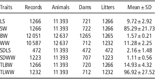
LS and survivability at weaning (SW) for each parturition were recorded across the experiment. Individual BW and WW was also recorded across generations. Phenotypic standard deviations of LS (SDLS) within female, and standard deviations WW (SDWW) within litter, were also considered as traits and afterwards analysed. Note that only two records of LS were used to calculate SDLS when available, and that single litters of the same female were used to analyse LS, but removed to analyse SDLS. Finally, total litter weight at birth (TLBW) and total litter weight at weaning (TLWW) were also registered to simultaneously account for, in a unique integrated trait, LS and BW in the TLBW and LS, WW and SW in the TLWW. The mean of the traits and number of records are shown in Table 1. The pedigree file contained 12 637 records including five generations of the panmictic population.
Number of records, animals in the pedigree, dams, litters and mean and standard deviation for eight analysed traits

LS=litter size (newborns); SW=survivability at weaning (%); BW=birth weight (g); WW=weaning weight (g); SDLS=standard deviation of litter size (newborns); SDWW=standard deviation of weaning weight (g); TLBW=total litter birth weight (g); TLWW=total litter weaning weight (g).
Models
Three different models were used to analyse the traits. First, a classical homoscedastic model (Model HOm) was used to estimate variance components and to predict breeding values for LS, SW, WW, SDLS, SDWW, TLBW and TLWW with the following equation:
 $$y_{i} \,{\equals}\,{\bf{x}} _{i} {\bf{b{\plus}w}} _{i} {\bf{m{\plus}v}} _{i} {\bf{c{\plus}e}} $$
where y
i
is either LS, SW, WW, SDLS, SDWW, TLBW or TLWW of the individual i, b the vectors of the systematic effects; m the vector of the direct genetic effect of the female (the mother when the record belongs to the pup) and c (not fitted for SDLS) the vector for the permanent environmental effect (litter effect for WW); x
i
, w
i
and v
i
are the incidence vectors for systematic, animal and permanent effects, respectively. The genetic effect m is Gaussian with
 $${\bf{m}} \!\sim\!N\left( {{\bf{0}} ,{\bf{A}} \sigma _{m}^{2} } \right)$$
, where A is the additive genetic relationship matrix and
 $$\sigma _{m}^{{\rm 2}} $$
is the additive genetic variance of the female effect, the vector c is assumed to be independent, with
 $${\bf{c}} \!\sim\!N\left( {\bf{0}} ,\,{\bf{I}} _{{\bf{c}} } \sigma _{c}^{2} } \right)$$
where I
c
is the identity matrix of equal order to the number of mothers and
 $$\sigma _{c}^{2} $$
is the permanent environmental variance, and the vector e is assumed to be independent, with
 ${\bf{e}} \!\sim\!N\left( {0,\,{\bf I}\sigma _{e}^{2} } \right)$
, and
 $$\sigma _{e}^{2} $$
is the residual variance. The fitted systematic effects were the same across models and are described below.
The second model was a homoscedastic direct-maternal animal model (Model HOi) that was used to analyse BW and WW:
 $$y_{i} \,{\equals}\,{\bf{x}} _{i} {\bf{b{\plus}w}} _{i} {\bf{m{\plus}v}} _{i} {\bf{c{\plus}e}} $$
with all the model definitions as the previous model, but a being the vector of the direct genetic effect of the pup and m the maternal genetic effect of its dam, c the vector for the maternal permanent environmental effect; z i , w i and v i are the incidence vectors for a, m and c, respectively. The genetic effects a and m are Gaussian with
 $$\left[ {\matrix{ {\bf a} \cr {\bf m} \cr } } \right]\,\sim\,N\left( {\left[ {\matrix{ {\bf 0} \cr {\bf 0} \cr } } \right],\left[ {\matrix{ {{\bf A}\sigma _{a}^{2} } & {{\bf A}\sigma _{{am}} } \cr {{\bf A}\sigma _{{am}} } & {{\bf A}\sigma _{m}^{2} } \cr } } \right]} \right)$$
where A is the additive genetic relationship matrix and
 $\sigma _{a}^{2} $
and
 $\sigma _{m}^{2} $
are, respectively, the direct and maternal additive genetic variances and
 $\sigma _{{am}} $
the genetic covariance between both genetic effects.
The third model was the heteroscedastic model (Model HE) developed by SanCristobal-Gaudy et al. (Reference SanCristobal-Gaudy, Elsen, Bodin and Chevalet1998) which assumes that the environmental variance is heterogeneous and partially under genetic control, and was used to analyse LS and WW traits:
 $$y_{i} \,{\equals}\,{\bf x}_{i} {\bf b}{\plus}{\bf w}_{i} {\bf m}{\plus}{\bf v}_{i} {\bf c}{\plus}e^{{{\raise0.5ex\hbox{$\scriptstyle 1$}\kern-0.1em/\kern-0.15em\lower0.25ex\hbox{$\scriptstyle 2$}}\left( {{\bf x}_{i} {\bf b}{\asterisk}{\plus}{\bf w}_{i} {\bf m}{\asterisk}{\plus}{\bf v}_{i} {\bf c}{\asterisk}} \right)}} {\epsilon}_{i} $$
where y
i
is either LS of the female i and WW of the mother i of the pup, * indicates the parameters associated with environmental variance; b and b* are the vectors of the systematic effects; m and m* the vectors of the direct genetic effect of the mother, and c and c* the vectors of the litter effect; x
i
, w
i
and v
i
are the incidence vectors for systematic, animal and litter effects, respectively. Finally,
 ${\epsilon}_{i} \!\sim\!N(0,1)$
. The genetic effects m and m* are distributed together and are assumed to be Gaussian:
 $$\left[ {\matrix{ {\bf m} \cr {{\bf m}{\asterisk}} \cr } } \right]\,\sim\,N\left( {\left[ {\matrix{ {\bf 0} \cr {\bf 0} \cr } } \right],\left[ {\matrix{ {\sigma _{m}^{2} } & {\rho \sigma _{m} \sigma _{{m{\asterisk}}} } \cr {\rho \sigma _{m} \sigma _{{m{\asterisk}}} } & {\sigma _{{m{\asterisk}}}^{2} } \cr } } \right]\,\otimes\,{\bf A}} \right)$$
where A is the additive genetic relationship matrix;
 $\sigma _{m}^{2} $
the maternal additive genetic variance of the trait;
 $\sigma _{{m{\rm {\asterisk}}}}^{2} $
the maternal additive genetic variance affecting environmental variance of the trait; ρ the coefficient of genetic correlation; and ⊗ denotes the Kronecker product. The vectors c and c* are also assumed to be independent, with
 ${\bf{c}} \!\sim\!N\left( {0,{\bf{I}} _{{\bf{c}} } \sigma _{c}^{2} } \right)$
and
 ${\bf{c}} ^{{\rm {\asterisk}}} \!\sim\!N\left( {0,{\bf{I}} _{{\bf{c}} } \sigma _{{c^{{\rm {\asterisk}}} }}^{2} } \right)$
where I
c
is the identity matrix of equal order to the number of litters and
 $\sigma _{c}^{2} $
and
 $\sigma _{{c{\asterisk}}}^{2} $
are the litter effect variances affecting, respectively, the mean of the trait and its environmental variability (Ibáñez-Escriche et al., Reference Ibáñez-Escriche, García and Sorensen2008). The systematic effects (b and/or b*) of the applied models included generation (eight levels), LS (from 2 to 17, 16 levels) except for LS and SDLS, sex (male and female for WW and also unknown for BW) and parity number (two levels). There were 1232 levels of permanent environmental effects (c) with 1232 levels of litters, and 12 637 levels of additive genetic effects or 11 393 when traits were assigned to the mother. Model HE was used in the experiment with data from Formoso-Rafferty et al. (Reference Formoso-Rafferty, Cervantes, Ibáñez-Escriche and Gutiérrez2015) to predict the breeding values for BW environmental variability.
Genetic parameters under both models HOm and Hoi were estimated by using TM software (Legarra, Reference Legarra2008). The Model HE was fitted by using the GSEVM programme (Ibáñez-Escriche et al., Reference Ibáñez-Escriche, Moreno, Nieto, Piqueras, Salgado and Gutiérrez2010). The results for each model were computed by averaging the results obtained from chains of Monte Carlo (Markov chain Monte Carlo (MCMC)) samples after running 1 000 000 iterations sampling one of each 100 iterations, and discarding the first 100 000. Genetic trends for the three models were analysed by averaging the predicted breeding values within line and generation and plotting them against generation.
For statistical inferences, LS, SW, WW, SDLS, SDWW, TLBW and TLWW were also analysed under a simple least squared model:
 $$y_{i} \,{\equals}\,{\bf x}_{i} {\bf b}{\plus}e_{i} $$
in which y i was either one of LS, SW, WW, SDLS, SDWW, TLBW or TLWW, and systematic effects in b were line×generation (17 levels) instead of generation, and the other systematic effects as described above, except TLBW and TLWW in which LS was excluded given that there were differences in mean LS between lines. Marginal posterior distributions of the difference between solutions for different lines, but ‘same generation’ were drawn to infer probabilities of response.
Results
Genetic parameters
Table 2 shows the estimated genetic parameters for the involved traits under a variety of models according to the analysed trait. Maternal heritabilities from Model HOm ranged from 0.06 for SW to 0.34 for SDLS. Variance components at the trait level were consistent between Model HOm and HE for LS and WW, the traits fitted under both models. The genetic variance concerning the environmental variability of WW and LS fell within the range reviewed by Hill and Mulder (Reference Hill and Mulder2010). Genetic correlation between the trait and the environmental variability levels was −0.33 for WW and −0.81 for LS. Direct and maternal heritabilities as well as c 2 were computed as the ratio between the respective variance component and the phenotypic variance estimated under Model HOi. Direct and maternal heritabilities were, respectively, 0.07 and 0.16 for WW, and 0.15 and 0.07 for BW, with a direct-maternal genetic correlation of 0.19 for BW and almost null for WW (−0.02).
Mean (and standard deviation) of the marginal posterior distribution for the additive genetic variance (
 $\sigma _{a}^{2} $
), maternal genetic variance affecting the mean and its variation (
 $\sigma _{m}^{2} $
and
 $\sigma _{{m{\asterisk}}}^{2} $
), the litter (or permanent for BW and WW) variances affecting the mean and its variation (
 $$\sigma _{c}^{2} $$
and
 $\sigma _{{c{\asterisk}}}^{2} $
), their genetic correlation (
 $\rho _{{mm{\asterisk}}}^{{}} $
),the direct-maternal genetic covariance (
 $\sigma _{{am}}^{{}} $
) and correlation (
 $\rho _{{am}}^{{}} $
), the direct and maternal heritabilities (h
2 and m
2) and the ratio between the litter (or permanent) and phenotypic variance (c
2), under models heteroscedastic (Model HE), individual homoscedastic (Model HOi) or maternal homoscedastic (Model HOm)

BW=Individual birth weight; WW=weaning weight; LS=litter size; SDLS=litter size standard deviation; SDWW=weaning weight standard deviation; SW=survivability at weaning; TLWW=total litter weaning weight; TLBW=total litter birth weight.
Trends
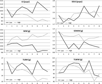
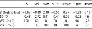
Figure 1 shows phenotypic trends for the traits LS, SDLS, WW, SDWW, TLBW and TLWW across eight generations of selection. All of them performed irregularly across generations. However, a clear divergence between lines for LS and WW was exhibited, whereas for SDLS this was erratic with no clear differences between lines. Regarding the other traits, the low line had a higher performance than the high line for TLBW and TLWW, but lower for WW and SDWW. Looking at the marginal posterior distribution of the difference in the performance between the two lines in the last generation, the probability of these differences being higher (for WW and SDWW) or lower (LS, SW, SDLS, TLBW and TLWW) than zero were 100% for LS, 62% for SW, 100% for WW, 90% for SDLS, 100% for SDWW, 96% for TLBW and 25% for TLWW (Table 3).
Phenotypic trends of litter size (LS), standard deviation of litter size (SDLS), weaning weight (WW), standard deviation of weaning weight (SDWW), total litter birth weight (TLBW) and total litter weaning weight (TLWW) across eight generations of selection.

Mean (D), standard deviation, and probability of D>0 or D<0 (P%) of the marginal posterior distribution of the difference between high and low environmental variability lines at the last generation for litter size (LS), survivability at weaning (SW), weaning weight (WW), litter size standard deviation (SDLS), weaning weight standard deviation (SDWW), total litter weaning weight (TLWW) and total litter birth weight (TLBW)

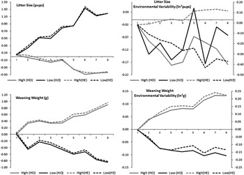
LS, WW, SDLS and SDWW were analysed each under Model HO. LS and WW were also analysed with its respective environmental variability under Model HE. The evolution of LS and WW at the trait level can be assessed by the genetic trend from either HO and HE models, and their evolution at the environmental variability level can be addressed by either the genetic trend of SDLS and SDWW under the Model HO, and the genetic trend at the variability level of SD and WW under the Model HE. Figure 2 shows these comparisons by drawing together the genetic trends at the trait level of both models HO and HE across eight generations of selection. In the same Figure 2, genetic trends for SDLS and SDWW under Model HO are shown together with the corresponding trends at the environmental variability level of LS and WW when analysed under Model HE. The trends were almost identical across models for LS and WW at the trait level. There was a clear divergence between lines with the low line having a better performance for LS but worse for WW. However, the models performed very differently at the environmental variability level depending on the trait. Although this trend for WW under Model HE was virtually identical to that of the SDWW under Model HO, the same comparison for LS showed big differences between models leading to complete different conclusions. Figure 2 also shows how WW at both trait and environmental variability levels evolved in the same direction in agreement with that observed for BW (Formoso-Rafferty et al., Reference Formoso-Rafferty, Cervantes, Ibáñez-Escriche and Gutiérrez2015). This was despite the genetic correlation between the WW mean and its environmental variability was negative,−0.33 (Table 2), unlike BW.
Genetic trends of the mean (left) of litter size (top) and weaning weight (bottom) and their respective environmental variability (right) by fitting Homoscedastic (HO) and Heteroscedastic (HE) models across eight generations of selection.

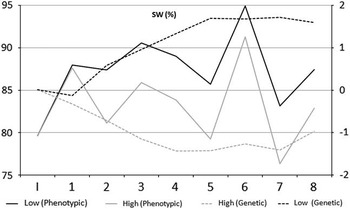
Phenotypic and genetic trends for SW are shown in Figure 3. The low line showed superiority in both trends. The phenotypic difference between lines was in fact obtained in the second generation and held across generations, with a throughout slope of 0.29 points of percentage per line and generation. From the genetic trends perspective, this slope was 0.16 points of percentage in the same period. The phenotypic trend exhibited a very important environmental influence of the generation effect but keeping the superiority of the low line along the whole experiment.
Genetic (right axis) and phenotypic (left axis) trends of the percentage of survivability at weaning (SW) across eight generations of selection.

Information about the marginal posterior distribution of the difference between lines at the last generation, considering LS, SW, WW, SDLS, SDWW, TLBW and TLWW traits, is shown in Table 3. The results tended to lead to the same conclusion previously obtained from the genetic trends. Thus, to a greater or lesser extent, the low line performed better than the high line for LS, SW and SDWW (lower values) but worse for WW, by not showing any superiority of the lines for SDLS. As a combination of the performance of these traits, the low line also performed higher for TLBW. Phenotypic trends showed that TLBW and TLWW were higher in the low line for both traits across generations except TLWW in the last generation in which the low line was 3% lower.
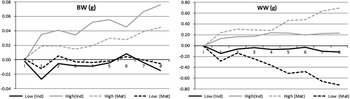
As the selection was based on BW environmental variability as a maternal trait, we checked whether genetic trends for BW and WW had a similar pattern when these traits were assigned to the individual. Figure 4 shows the individual and maternal genetic trends when data were analysed under a model involving both effects. Divergence was observed in the same direction for both genetic effects showing a superiority of the high line. Even though a practically null genetic correlation between direct and maternal genetic effects, both showed genetic response as a consequence of their genetic correlation with the selection objective, the BW environmental variability.
Direct (Ind) and maternal (Mat) genetic trends for birth weight (BW) and weaning weight (WW) across eight generations of selection.

Discussion
Formoso-Rafferty et al. (Reference Formoso-Rafferty, Cervantes, Ibáñez-Escriche and Gutiérrez2015) showed that selection for BW environmental variability was a successful process, but they did not show its implications on other production traits. Therefore, before applying this experience to livestock, the impact on some other welfare and productive traits should have to be addressed. In this paper, the correlated genetic trends affecting such other interesting traits were studied.
First, genetic parameters were estimated. In this case, most of the estimates were obtained by using maternal models because previously published results (Pun et al., Reference Pun, Cervantes, Nieto, Salgado, Pérez-Cabal, Ibáñez-Escriche and Gutiérrez2013) showed the convenience of analysing BW environmental variability as a maternal trait. The maternal heritability obtained for the traits were within the range of previous results published on mice (Ibáñez-Escriche et al., Reference Ibáñez-Escriche, García and Sorensen2008). The estimate of maternal heritability for SW was slightly lower than the value of 0.10 reported in pigs (Mesa et al., Reference Mesa, Safranski, Cammack, Weaber and Lamberson2006).
BW and WW were also analysed under direct-maternal animal models due to its important individual genetic base and to see how selecting mothers would impact on the evolution of the direct genetic effect. When comparing estimated parameters for WW across models, it should be remembered that in the maternal model, the maternal effect is also gathering half the individual direct effect, and maternal variance also gather a quarter of the individual additive genetic variance. Results were not completely equivalent given that a direct-maternal genetic covariance was also fitted. This led to a greater reduction of the maternal variance component but increasing the litter variance component.
Genetic correlation estimates between direct and maternal effects for WW and BW were low. These results are in contrast with usual high negative genetic correlations found in the literature (Cervantes et al., Reference Cervantes, Gutiérrez, Fernández and Goyache2010). Specifically, this genetic correlation found for WW suggests that genetic trends in this population would be expected to be independent in both genetic effects. However, looking at Figure 4, both genetic trends evolve in the same direction, with this evolution being roughly proportional to the variance of the effect. This would suggest that the selection criterion, the BW environmental variability, was correlated with both direct and maternal WW genetic effects. The mean WW was 2.10 g heavier in the high line than in low line, at the end of the selection process (Table 3). Looking at Figure 4, this superiority would be caused mainly by the maternal effect (Eisen, Reference Eisen1978). These trends were in agreement with other authors (Eisen, Reference Eisen1978; Bayon et al., Reference Bayon, Fuente and San Primitivo1987).
A detail worth mentioning refers to the performance of Model HE that virtually had identical genetic trends than the Model HO at the trait levels for both LS and WW. However, Figure 2 shows the different performance of models HO and HE for LS and WW on the variability level. On this level, the performance of the Model HE was fairly similar to that of Model HO for WW but very different for LS. There are several differences between SDWW and SDLS that explain the different performances of the model. The number of records for SDLS and SDWW were, respectively, 472 and 1223, and that standard deviation was computed with only two records in the first case, and with an average of 8.60 records in the second case. Standard deviations were poorly computed within individuals with two records at maximum. Then the phenotypic values, the genetic values and the corresponding trends were badly estimated. As a consequence, genetic correlation between the trait and environmental variability levels of LS was also poorly estimated. In this case this correlation resulted in a extreme negative value (−0.81), conditioning a highly related but inverse genetic trends between both levels. Thus, the genetic trend at the environmental variability level (Figure 2) became dramatically different from that of SDLS under Model HO (Figure 2), and also different from the phenotypic trend (Figure 1). A second conclusion can be drawn from this study. It has been shown that predicted breeding values for the environmental variability are unreliable with insufficient information under Model HE. However, in the scenario in which data provide enough information, both approaches perform mostly equal. Theoretically, there are more benefits in Model HE. It can simultaneously fit systematic effects on the trait and variability levels in one step, and it takes into account the whole structure of the data by using one residual per observation instead of one record per individual. Therefore, it would be theoretically preferred, but both models perform similarly in practice under robust information. The results show that the selection response evaluated with either models HO or HE are in good agreement. This can be considered as an argument in favour of the results found under Model HE, and therefore also in favour of the genetic parameters used in the analysis of the process of selection (García et al., 2009).
The positive relationship between the phenotypic and genetic trends of WW with its environmental variability (Figure 2) contradicted the obtained negative genetic correlation between them (−0.33, Table 2). Computed genetic correlation between predicted breeding values of the trait and the variability for WW, not shown, resulted negative within line and generation, but both genetic correlations between them and the selection criterion, the breeding value for the variability level of BW, were positive. It was a welcome surprise to realise how the negative genetic correlation could be bypassed to obtain both indirect genetic trends in the same direction by using as criterion a third positive genetically correlated trait. An interesting implication of this would be that selecting for reducing WW variability would lead to favourable response in both levels, increasing the WW mean and reducing its variability. There was therefore, a relationship between the variability at birth and at weaning. It could be partially explained because, in the low line, pups tend to weigh all the same at birth, having less competition for sucking, and tending to have consequently the same growth.
The experiment was carried out as a model for livestock species. Therefore, consequences on productivity and welfare are a concern. Regarding the consequences of selecting for BW environmental variability, the low line was clearly better for LS and SW. For the case of SW, and from a phenotypic point of view it seems that a strong response occurred at generation 2 and the difference between lines was maintained later on, but did not change under selection. Even this superiority was clear, the evolution was not always growing across generations and its magnitude varied depending on the method used to address it. There were identical genetic and phenotypic trends of 0.1 pups per line and generation with a final total rough difference of 1.65 pups between lines.
All these traits have been shown in the past to be related. Selection for LS should be accompanied by selection for mortality and/or BW traits. Losses from birth to weaning and the minimal BW in the litter were proposed as potential traits for selection against piglet mortality (Damgaard et al., Reference Damgaard, Rydhmer, Lovendahl and Grandinson2003; Wolf et al., Reference Wolf, Žakova and Groeneveld2008). The effect of LS on mortality and growth can be reduced markedly in homogeneous litters, which results in more efficient growth in rabbits of low BW. In addition, heterogeneous litters would be more prone to diseases that infect other pups in the same litter (Poigner et al., Reference Poigner, Szendrö, Levai, Radnai and Biro-Nemeth2000). However, grading BW and fostering methods would improve preweaning survival (Perrier, Reference Perrier2003). The results reported by García and Baselga (2002) indicate that selection for LS at weaning offers a tool to improve reproductive traits for weaning in rabbits, improving significantly ovulation rate, without significant negative changes in prenatal survival.
Thus, low line performed better for LS and SW with the consequent benefits in productivity and welfare. García et al. (Reference García, Argente, Muelas, Birlanga and Blasco2012) tested the hypothesis that in the rabbit a selection for LS residual variance affected animal welfare. This was partially confirmed in the present study. However, the mice in the low line were smaller both at birth and at weaning, which would be accompanied by a lower economic benefit and for some the state of their welfare might be worse. Thus, for example, thinking of the sale of animals at weaning, after eight generations of selection, a weaned animal from the high line weighed 26% more than one from the low line (12.72 v. 10.09 g). Although the animals were selected based on the performance of their mothers, both genetic trends, direct and maternal, were growing through generations. This difference could have been due in part to increased LS of the low line.
Summarising, considering LS and survival, low line was preferable from the welfare perspective, but its superiority from the productivity point of view was not clear. On the one hand the low line performed a higher LS and SW but with animals weaned with lower weight. However, the low line did not perform less total weight as shown by the final TLWW after eight generations.
It seems that robustness was higher in the low line as understood by Mormede and Terenina (Reference Mormede and Terenina2012) as less sensitivity with respect to environmental effects as indicated by a low variation having benefits in the animal welfare, but this still remains unclear. Other researches, for example, on growth after weaning, lifetime, number of weaned offspring during an uncensured life and responses to environmental changes should be carried out in order to understand robustness better.
Acknowledgements
This paper was partially funded by a grant from the Spanish Government (AGL2008-00794). The experiment will be continued with partial funding of Feed-a-gene and a grant from MEC-INIA (RTA2014-00015-C02-01). The authors wish to thank the detailed work of an anonymous reviewer who has contributed greatly to improving this work.