1. Introduction
The flow in the atmospheric boundary layer (ABL) critically affects several aspects of human activity, including weather, air quality, building and town-planning architecture, agriculture, and wind energy extraction (Stull Reference Stull2012; Mondal et al. Reference Mondal, Kethavath, Abhinay and Ghaisas2023). A prominent numerical methodology used to study turbulence in the ABL is large-eddy simulations (LES) of the Navier–Stokes equations, where only large-scale eddies are resolved, and the effects of the subgrid-scale (SGS) eddies are modelled (Stoll et al. Reference Stoll, Gibbs, Salesky, Anderson and Calaf2020). Specific LES techniques can be categorised into wall-resolved LES (WRLES) and wall-modelled LES (WMLES) types, depending on the near-wall treatment and the numerical resolution of the wall viscous scale. Since WRLES are presently limited to moderate Reynolds numbers owing to prohibitively high computational costs (Piomelli & Balaras Reference Piomelli and Balaras2002), simulations of high-Reynolds-number ABL flows rely heavily on SGS and wall modelling (Liu & Stevens Reference Liu and Stevens2020; Gadde, Stieren & Stevens Reference Gadde, Stieren and Stevens2021).
The most widely used SGS modelling method is the Smagorinsky model (Smagorinsky Reference Smagorinsky1963), in which the SGS stresses are parametrised using the eddy viscosity concept. The model coefficient
 $C_{s, \varDelta }$
at grid scale
 $\varDelta$
is derived from theoretical arguments and empirical formulations (Lilly Reference Lilly1967). The Smagorinsky model is usually applied to the LES of ABL flows combined with a wall damping function, such as the Mason wall damping function (Mason & Thomson Reference Mason and Thomson1992), which can be overly dissipative near the surface (Porté-Agel et al. Reference Porté-Agel, Meneveau and Parlange2000). This drawback is overcome by calculating
 $C_{s, \varDelta }$
dynamically based on the relation between the SGS stresses at different scales (typically, grid scale
 $\varDelta$
and test-filter scale
 $2\Delta$
) (Germano et al. Reference Germano, Piomelli, Moin and Cabot1991). To account for scale effects and heterogeneous surfaces of geophysical flows, Bou-Zeid, Meneveau & Parlange (Reference Bou-Zeid, Meneveau and Parlange2005) proposed the Lagrangian-averaged scale-dependent dynamic (LASD) model, combining scale-dependent refinement (Porté-Agel et al. Reference Porté-Agel, Meneveau and Parlange2000) and Lagrangian averaging (averaging over fluid path lines) (Meneveau, Lund & Cabot Reference Meneveau, Lund and Cabot1996). At a given grid resolution, this approach has proven capable of capturing the flow physics for neutral and both stably and unstably stratified boundary layers more effectively than does the Smagorinsky model (Gadde et al. Reference Gadde, Stieren and Stevens2021).
A further commonly used parametrisation for wall-bounded flows is the standard ‘equilibrium’ wall model based on the Monin–Obukhov similarity theory (Moeng Reference Moeng1984), which estimates the mean wall shear stress magnitude by inverting the logarithmic law of the wall; this model is referred to as the log-law (LL) model. The pure LL model encounters theoretical limitations in flows over heterogeneous rough surfaces, as horizontal averaging becomes invalid in such flows (Mondal et al. Reference Mondal, Kethavath, Abhinay and Ghaisas2023), making its predictive performance highly dependent on the chosen SGS model. To address this limitation, Abkar & Porté-Agel (Reference Abkar and Porté-Agel2012) developed a new boundary condition for LES of ABL flows over surface-roughness transitions. By incorporating a blending function, this model explicitly accounts for streamwise variations in local friction velocity, and their gradual approach to equilibrium values. Although effective on heterogeneous surfaces, this model requires specifying the internal boundary layer (IBL) – formed downstream of roughness transitions and growing vertically with streamwise distance – as an input parameter. Specifically, it requires the ratio of internal equilibrium layer (IEL, the IBL sublayer fully adjusted to local roughness) height to total IBL height.
The WMLES conducted by Yang & Bose (Reference Yang and Bose2017), Wang, Hu & Zheng (Reference Wang, Hu and Zheng2020) and Feng et al. (Reference Feng, Gupta, Li and Wan2024) demonstrate that the mean streamwise velocity and velocity variances in turbulent flows over smooth or homogeneous rough surfaces are insensitive to wall models, confirming that the LL model is sufficiently accurate as a benchmark for WMLES of ABLs over homogeneous surfaces. However, in WMLES of ABLs over heterogeneous surfaces with roughness transitions, wall models significantly affect the wall skin friction and outer region turbulence fluctuations, as shown by Mondal et al. (Reference Mondal, Kethavath, Abhinay and Ghaisas2023) and Abkar & Porté-Agel (Reference Abkar and Porté-Agel2012). This motivates the need for a parameter-free wall-modelling methodology for simulating ABL flows.
Structure-based concepts offer an alternative to phenomenological SGS and WMLES. The stretched vortex (SV) model (Misra & Pullin Reference Misra and Pullin1997) does not utilise specific filtering operations but instead explicitly represents subgrid motion within each computational cell using nearly axisymmetric stretched vortices aligned with either the local resolved strain rate tensor or a weighted mix of this with the resolved vorticity vector. The SV approach was extended by Chung & Matheou (Reference Chung and Matheou2014) to simulate buoyancy-stratified turbulence, and subsequently tested in both stably and unstably stratified flows (Matheou & Chung Reference Matheou and Chung2014).
Quasi-streamwise vortical structures in the overlap region of wall-bounded turbulence can be captured by the SV model as an ensemble of vortices aligned in the streamwise direction, providing natural advantages for simulating wall-modelled turbulence. Chung & Pullin (Reference Chung and Pullin2009) coupled this ansatz with the integral of the filtered momentum equation and semi-implicit, inner scaling of near-wall turbulence, to build a non-equilibrium wall model that describes wall shear stress evolution via an ordinary differential equation (ODE). The ODE solution then enables a Dirichlet slip velocity boundary condition at a raised, flat virtual wall, forming the virtual-wall model (VWM). The SV-VWM has been utilised for LES of various wall-bounded flows, including smooth (Chung & Pullin Reference Chung and Pullin2009) and rough (Saito, Pullin & Inoue Reference Saito, Pullin and Inoue2012; Saito & Pullin Reference Saito and Pullin2014) turbulent channel flows, smooth (Inoue & Pullin Reference Inoue and Pullin2011) and rough (Sridhar, Pullin & Cheng Reference Sridhar, Pullin and Cheng2017) turbulent boundary layers (TBLs), and smooth TBL separation (Cheng, Pullin & Samtaney Reference Cheng, Pullin and Samtaney2015). The performance of the SV-VWM model in LES of shear-dominated, neutral ABL flows over rough homogeneous or heterogeneous surfaces remains untested.
The main objective of this study is to extend the simulation capability of the SV-VWM model for effective LES of neutral ABL flows. The VWM is partially parametrised by the wall-normal displacement of the virtual wall, determined by Chung & Pullin (Reference Chung and Pullin2009) as a fixed fraction of the wall-adjacent cell height. To eliminate both this and other model parameters – such as the offset used in the Dirichlet, slip velocity boundary condition – we retain the friction velocity (
 $u_\tau$
) ODE component, but replace the slip velocity with a wall stress boundary condition. An eddy viscosity is not required. This approach eliminates the virtual wall requirement, and potentially simplifies applications to complex geometries. The improved model is termed the wall-stress ODE (WSODE) model.
In the following, the WSODE is coupled with the SV SGS model, denoted the SV-WSODE combination, and is applied to neutral ABL LES over both rough homogeneous and heterogeneous surfaces. The benchmark model employed is the LASD model, which has been successfully applied to ABL flow simulations. The paper is organised as follows. The numerical methodology and models studied are detailed in § 2. Case set-up details and simulation results are analysed and compared with experimental results in §§ 3 and 4. Concluding remarks are summarised in § 5.
2. The LES methodology
2.1. Numerical method
The generically filtered non-dimensional incompressible Navier–Stokes equations are
 \begin{equation} \begin{aligned} \frac {\partial \widetilde {u}_i}{\partial t}+\widetilde {u}_{\!j}\left (\frac {\partial \widetilde {u}_i}{\partial x_{\!j}}-\frac {\partial \widetilde {u}_{\!j}}{\partial x_i}\right )=-\frac {\partial \widetilde {p^*}}{\partial x_i}+ \frac {\partial }{\partial x_{\!j}} \left (\nu \frac {\partial \widetilde {u}_i}{\partial x_{\!j}}-\tau _{\textit{ij}}\right )+\delta _{1i}f_i, \quad \frac {\partial \widetilde {u}_i}{\partial x_i}=0, \end{aligned} \end{equation}
where
 $\widetilde {u}_i$
denotes the filtered velocity component, with subscripts
 $i=1,2,3$
corresponding to the streamwise
 $(\widetilde {u})$
, spanwise
 $(\widetilde {v})$
and vertical
 $(\widetilde {w})$
components;
 $\nu$
is the kinematic viscosity. The SGS stress tensor is given by
 $\tau _{\textit{ij}}=\widetilde {u_i u_{\!j}}-\widetilde {u}_i\widetilde {u}_{\!j}$
. Currently, no explicit spatial filtering is applied to the physical grid. The convection term employs the rotational form to conserve kinetic energy and mass, yielding the modified pressure
 $\widetilde {p^*}=\widetilde {p}/{\rho }+1/2\widetilde {u}_{\!j} \widetilde {u}_{\!j}$
, where
 $\widetilde {p}$
is the resolved pressure, and
 $\rho$
is the fluid density. Viscous and subgrid stresses are combined into the total stress
 $\tau _{\textit{ij}}^{\textit{tot}}=\nu\, {\partial \widetilde {u}_i}/{\partial x_{\!j}}-\tau _{\textit{ij}}$
. The forcing term
 $f_i$
drives the flow, and
 $\delta _{\textit{ij}}$
denotes the Kronecker delta. Since neutral stability conditions are considered, buoyancy effects are excluded (Porté-Agel et al. Reference Porté-Agel, Meneveau and Parlange2000). The Coriolis term is neglected, as the study focuses on flow physics within a
 $300\ \mathrm{m}$
ABL (Bou-Zeid, Meneveau & Parlange Reference Bou-Zeid, Meneveau and Parlange2004).
The governing equations are solved in a computational domain of dimensions
 $L_x \times L_y \times L_z$
(the streamwise, spanwise and vertical directions, respectively). The domain is discretised into
 $N_x$
,
 $N_y$
and
 $N_z$
grid points, with grid spacings
 $\Delta x=L_x/N_x$
,
 $\Delta y=L_y/N_y$
and
 $\Delta z=L_z/N_z$
. The numerical solver is generally based on the high-fidelity parallel pseudo-spectral open-source code LESGO, which has been extensively validated for ABL flow studies (Albertson & Parlange Reference Albertson and Parlange1999; Porté-Agel et al. Reference Porté-Agel, Meneveau and Parlange2000; Bou-Zeid et al. Reference Bou-Zeid, Meneveau and Parlange2004, Reference Bou-Zeid, Meneveau and Parlange2005). It uses a pseudo-spectral method with periodic boundary conditions in horizontal directions, combined with a second-order central difference scheme in the vertical direction. Time integration employs a second-order-accurate Adams–Bashforth scheme. Aliasing errors resulting from the nonlinear terms are prevented via the
 $3/2$
anti-aliasing rule (Hussaini & Zang Reference Hussaini and Zang1986). Refer to Albertson (Reference Albertson1996) and Albertson & Parlange (Reference Albertson and Parlange1999) for further details of LESGO. The ABL flow simulations employ a half-channel configuration. At the top boundary, zero vertical velocity and stress-free conditions are imposed, while the viscous effects at the bottom surface are captured by wall models. The computational domain configuration is schematised in figure 1.
Schematic of the computational domain and the boundary conditions. The bottom surface is divided into three patches with different wall roughnesses, where the first patch is referred to as the upstream patch and has roughness
 $z_{01}$
, and the second patch is referred to as the downstream patch and has roughness
 $z_{02}$
. The third patch has the same roughness
 $z_{01}$
as the first patch, so the periodic condition is fulfilled in the streamwise direction. For a rough homogeneous surface,
 $z_{01}=z_{02}=z_{0}$
.

Owing to the high Reynolds number of atmospheric flows and the fact that the viscous sublayer is not resolved in the present LES, the viscous term is negligible in the numerical solution of the resolved-scale equations (Porté-Agel et al. Reference Porté-Agel, Meneveau and Parlange2000; Bou-Zeid et al. Reference Bou-Zeid, Meneveau and Parlange2004, Reference Bou-Zeid, Meneveau and Parlange2005). However,
 $\nu$
is retained in both the SV model and the wall model, ensuring that finite Reynolds number effects in the overall LES are retained. In the present work, the SV SGS model and the WSODE are implemented in LESGO. The LASD model and the standard LL model, which have been developed in the code, serve as the benchmark SGS and wall models, respectively. Refer to Bou-Zeid et al. (Reference Bou-Zeid, Meneveau and Parlange2005) for the detailed formulation of this benchmark framework.
2.2. The SV SGS model
Unlike the typical eddy viscosity model, the SV SGS model directly models the full SGS stress tensor
 $\tau _{\textit{ij}}$
, thereby excluding the trace of the SGS stress tensor
 $\tau _{kk}$
from the modified pressure
 $\widetilde {p^*}$
. It is assumed that the subgrid vorticity in each cell comprises a superposition of vortices that may be stretched by the resolved-scale rate of strain tensor, each of which is unidirectional and of cylindrical type (Misra & Pullin Reference Misra and Pullin1997). The ensemble dynamics of SGS motion is further assumed to be dominated by a vortex aligned with a unit vector
 $\boldsymbol{e}^v$
, resulting in the subgrid stress tensor
 $\tau _{\textit{ij}}$
being modelled via a delta function probability density function as (Chung & Pullin Reference Chung and Pullin2009)
 \begin{equation} \begin{aligned} \tau _{\textit{ij}}=\big (\delta _{\textit{ij}}-e_i^v e_{\!j}^v\big) K, \quad K=\int _{k_c}^{\infty } E(k)\, \mathrm{d}k=\frac {1}{2} \mathscr{K}_0^{\kern3pt \prime } \varGamma \left [-\frac {1}{3}, \kappa _c^2\right ]\!, \end{aligned} \end{equation}
with
 $K$
the subgrid kinetic energy,
 $k_c=\pi / \varDelta _c$
the cut-off wavenumber,
 $k$
the wavenumber, and
 $E(k)$
the energy spectrum. In the integration above, the Lundgren vortex model (Lundgren Reference Lundgren1982) is used, with
 $\mathscr{K}_0^{\kern3pt \prime }=\mathscr{K}_0 \epsilon ^{2 / 3} \lambda _v^{2 / 3}$
, where
 $\epsilon$
is the local cell-averaged dissipation (resolved flow plus SGS). Here,
 $\varGamma$
is an incomplete Gamma function,
 $\kappa _c=k_c \lambda _v$
, and
 $\lambda _v=(2 \nu /(3\,|\widetilde {a}|))^{1/2}$
. The quantity
 $\widetilde {a}=e_i^v e_{\!j}^v \widetilde {S}_{\textit{ij}}$
represents the stretching along the subgrid vortex, where
 $\widetilde {S}_{\textit{ij}}= (1/2 ) (\partial \widetilde {u}_i / \partial x_{\!j}+\partial \widetilde {u}_{\!j} / \partial x_i )$
is the resolved strain rate tensor.
By using a matching procedure, the constant
 $\mathscr{K}_0^{\kern3pt \prime }$
can be found as
 $\mathscr{K}_0^{\kern3pt \prime }=\langle F_2\rangle / \langle Q(\kappa _c, d)\rangle$
. Here,
 $\langle {\cdot }\rangle$
denotes the local average computed technically from a set of 26 neighbouring points, and
 $F_2$
is the local second-order velocity structure function calculated from the resolved velocities. The quantity
 \begin{equation} \begin{aligned} Q\left (\kappa _c, d\right )=4 \int _0^{\kappa _c} \kappa ^{-5 / 3}\, \mathrm{e}^{-\kappa ^2}\left [1-J_0\left (\left (\kappa / \kappa _c\right ) \pi d\right )\right ] \mathrm{d} \kappa \end{aligned} \end{equation}
is calculated using an efficient asymptotic approximation with
 $d=r / \varDelta _c$
, and
 $r$
is the distance from the neighbour point to the vortex axis (Chung & Pullin Reference Chung and Pullin2009).
2.3. The WSODE model
The wall model discussed here is developed in the sense of wall integration (Chung & Pullin Reference Chung and Pullin2009; Inoue & Pullin Reference Inoue and Pullin2011; Saito et al. Reference Saito, Pullin and Inoue2012; Cheng et al. Reference Cheng, Pullin and Samtaney2015). Define wall-parallel filtering and wall-normal integration operators as
 \begin{align} \begin{aligned} \widetilde {\phi }(x, y, z, t)&=\iint \phi \left (x^{\prime }, y^{\prime }, z, t\right ) G\left (x-x^{\prime } ; \varDelta _{\!f}\right ) G\left (y-y^{\prime } ; \varDelta _{\!f}\right ) {\rm d} x^{\prime }\, {\rm d} y^{\prime }, \\ &{ \langle \widetilde {\phi }\rangle (x, y)=\frac {1}{h-k(x, y)} \int _{k(x, y)}^h \widetilde {\phi }(x, y, z)\, {\rm d} z,} \end{aligned} \end{align}
where
 $\widetilde {({\cdot })}$
denotes wall-parallel filtering, and
 $\langle {\cdot }\rangle$
represents wall-normal averaging. Here,
 $\varDelta _{\!f}$
represents the LES SGS length scale, which is much larger than the viscous length scale. We note the wall-parallel filter is formal and not implemented explicitly. The wall geometry is defined by
 $z=k(x, y)$
, and
 $h$
denotes the wall-integral height. Applying (2.4) to the streamwise momentum equation along with the no-slip condition
 $\widetilde {u}(x,y,k,t) = 0$
, and assuming that the streamwise pressure gradient is constant within the wall-integral layer, Saito et al. (Reference Saito, Pullin and Inoue2012) derive
 \begin{align} \begin{aligned} &\frac {\partial \langle \widetilde {u}\rangle }{\partial t}+\frac {\partial \langle \widetilde {u} \widetilde {u} \rangle }{\partial x}+\frac {\partial \langle \widetilde {u} \widetilde {v}\rangle }{\partial y}+\frac {\partial \langle \tau _{xx} \rangle }{\partial x}+\frac {\partial \langle \tau _{xy} \rangle }{\partial y} \\ &=-\left .\frac {1}{h} \widetilde {u} \widetilde {w}\right |_h -\left .\frac {1}{h} \tau _{xz}\right |_h -\left .\frac {\partial \widetilde {p}}{\partial x}\right |_h+f_1+\frac {\nu }{h}\left .\frac {\partial \widetilde {u}}{\partial z}\right |_h-\frac {1}{h} u_{\tau }^2, \end{aligned} \end{align}
where the subscript
 $h$
denotes the quantity evaluated at
 $z = h$
. The lateral diffusion has been neglected in (2.5), which is justifiably small, given the relative size of the filter width.
The semi-implicit inner-scaling ansatz, originally proposed by Chung & Pullin (Reference Chung and Pullin2009) for smooth-wall-bounded turbulence, and extended to rough-wall-bounded turbulence by Saito et al. (Reference Saito, Pullin and Inoue2012), is employed such that the unsteady term in (2.5) is expressed as
 \begin{equation} \begin{aligned} \frac {\partial \langle \widetilde {u}\rangle }{\partial t}=\left (\frac {\left .\widetilde {u}\right |_h}{u_\tau }-k_{s}^{+} \frac { {\rm d} \Delta U^{+}}{ {\rm d} k_{s}^{+}}\right )\frac {\partial u_\tau }{\partial t}\equiv F\frac {\partial u_\tau }{\partial t}, \end{aligned} \end{equation}
where
 $u_\tau = \sqrt {\tau _w / \rho }$
is the friction velocity, with
 $\tau _w$
and
 $\rho$
representing the wall shear stress and fluid density, respectively. Here,
 $F$
is referred to as the geometric factor. The detailed mathematical derivation extending the geometric factor
 $F$
from smooth-wall to rough-wall turbulence is provided in Appendix A. Here,
 $\Delta U^{+} = (1/\kappa ) \log (1+0.26 k_{s}^{+})$
is the Colebrook (Jiménez Reference Jiménez2004) roughness function, where
 $\kappa$
is the von Kármán constant,
 $k_{s}$
is the equivalent sand roughness, and
 $k_{s}^{+}=k_{s} u_{\tau }/{\nu }$
. Substituting (2.6) into (2.5) and adopting the nonlinear-term approximations
 \begin{equation} \begin{aligned} \frac {\partial \langle \widetilde {u} \widetilde {u} \rangle }{\partial x} \approx \frac {\partial \left . \widetilde {u} \widetilde {u}\right |_h}{\partial x}, \quad \frac {\partial \langle \widetilde {u} \widetilde {v} \rangle }{\partial y} \approx \frac {\partial \left . \widetilde {u} \widetilde {v}\right |_h}{\partial y}, \quad \frac {\partial \langle \tau _{xx} \rangle }{\partial x} \approx \frac {\partial \left . \tau _{xx}\right |_h}{\partial x}, \quad \frac {\partial \langle \tau _{xy} \rangle }{\partial y} \approx \frac {\partial \left . \tau _{xy}\right |_h}{\partial y}, \end{aligned} \end{equation}
an ODE for
 $u_{\tau }$
is obtained:
 \begin{align} \begin{aligned} &\frac { {\rm d} u_\tau }{ {\rm d} t}=\frac {1}{F}\left (-\frac {\partial \left . \widetilde {u} \widetilde {u}\right |_h}{\partial x}-\frac {\partial \left . \widetilde {u} \widetilde {v}\right |_h}{\partial y}-\frac {\partial \left . \tau _{xx}\right |_h}{\partial x}-\frac {\partial \left . \tau _{xy}\right |_h}{\partial y} \right. \\&\,-\left. \left .\frac {1}{h} \widetilde {u} \widetilde {w}\right |_h -\left .\frac {1}{h} \tau _{xz}\right |_h -\left .\frac {\partial \widetilde {p}}{\partial x}\right |_h+f_1+\frac {\nu }{h}\left .\frac {\partial \widetilde {u}}{\partial z}\right |_h-\frac {1}{h} u_{\tau }^2\right )\!. \end{aligned} \end{align}
Note that the tilde notation
 $\widetilde {({\cdot })}$
is used here to denote the two-dimensional wall-parallel filtering, which is formally distinct from the implicit three-dimensional LES filter used in (2.1). However, because no explicit filtering operations are performed in the present numerical framework, this planar filtering is purely formal (Chung & Pullin Reference Chung and Pullin2009). For the purposes of coupling the ODE (2.8) with the LES solver, the two-dimensional planar-filtered quantities are directly approximated by the three-dimensional LES resolved quantities evaluated at
 $z=h$
, allowing the variables in (2.8) to be evaluated directly using the corresponding LES fields. Furthermore, we emphasise that the present wall model always has a finite Reynolds number due to the existence of viscosity
 $\nu$
in the ODE (2.8). Variations in
 $\nu$
directly reflect the Reynolds number effect.
The integral height
 $h$
is set to
 $\Delta z/2$
. The ODE (2.8) is implemented at each wall-adjacent cell through the following procedure.
-
(i) Equation (2.8) is solved concurrently with the full LES time integration to estimate the instantaneous
 $u_{\tau }(x,y,t)$
field.
-
(ii) The wall-normal velocity gradient at
$z=h$
in the ODE (2.8) (second-last term inside the brackets on the right-hand side) is approximated using the logarithmic law of the wall, yielding
$\left .({\partial \widetilde {u}}/{\partial z})\right |_h \approx u_\tau /{(\kappa h)}$
, where
$\kappa$
is the von Kármán parameter, with good robustness, while the other terms on the right-hand side of (2.8) are obtained directly from the outer LES at
$z=h$
. -
(iii) The ODE requires information from the SGS model since it lacks information about the layer between the wall
$z=0$
and the wall-integral height
$z=h$
. Currently, the ODE is implemented in conjunction with the SV model (Chung & Pullin Reference Chung and Pullin2009; Inoue & Pullin Reference Inoue and Pullin2011; Saito et al. Reference Saito, Pullin and Inoue2012; Cheng et al. Reference Cheng, Pullin and Samtaney2015) to ensure accurate near-wall predictions. -
(iv) When
$u_\tau$
is obtained, the stress boundary condition is applied to the LES, based on the balance between wall shear stress
$u_\tau ^2$
and the near-wall fluid shear stress
$\tau _{xz}^{\textit{tot}}$
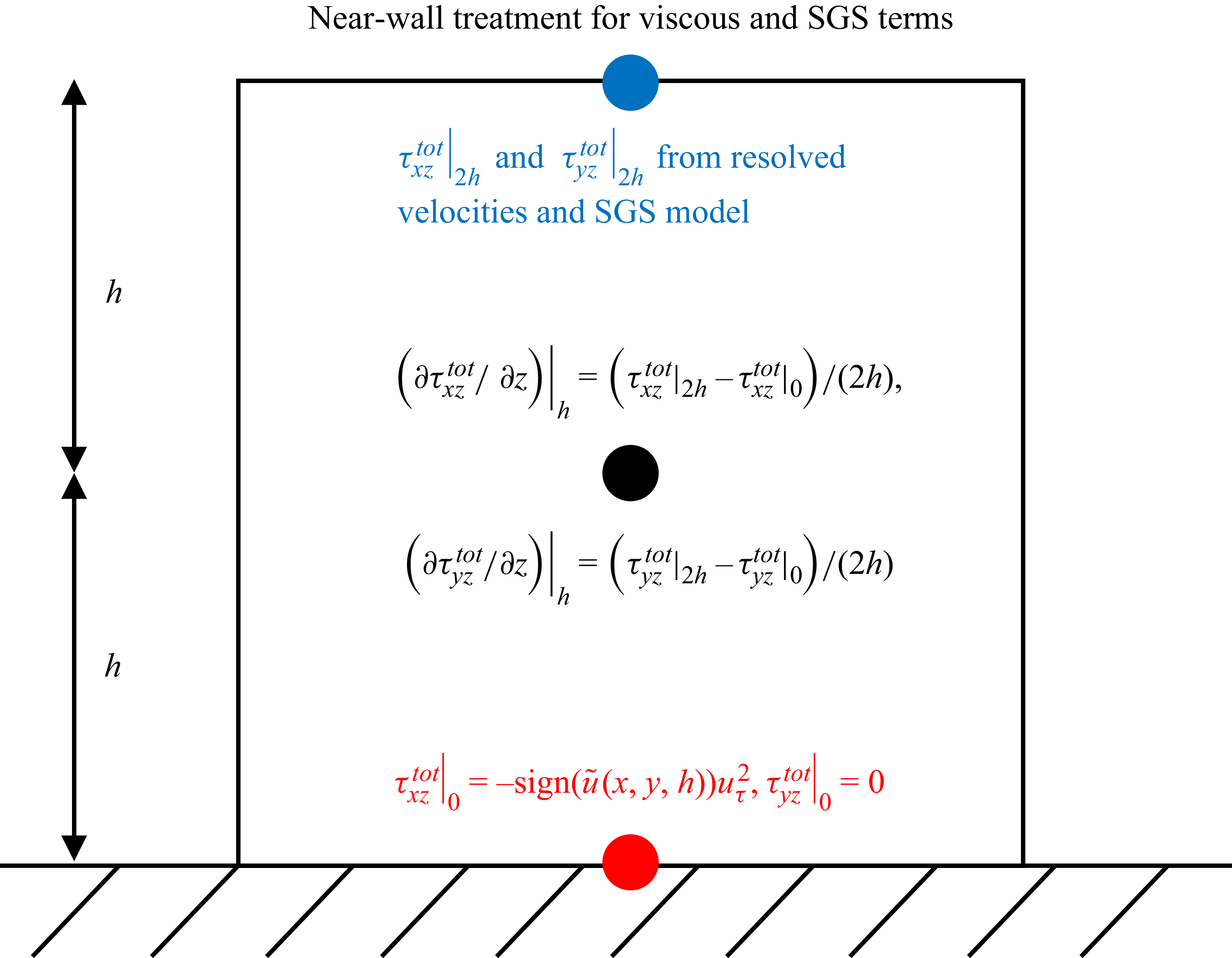
:(2.9)This closes the viscous and SGS terms at the half-cell near the wall, as shown in figure 2.
\begin{equation} \begin{aligned} \tau _{xz}^{\textit{tot}}(x, y, 0)=-\mathrm{sign}[{\widetilde {u}}(x, y, h)] \left [u_{\tau }(x, y)\right ]^2, \quad \tau _{yz}^{\textit{tot}}(x, y, 0) = 0. \end{aligned} \end{equation}


Chung & Pullin (Reference Chung and Pullin2009) determine
 $\kappa$
dynamically, but in step 2 above,
 $\kappa = 0.4$
is used for simplicity, which is the only numerical parameter of the wall model. The WMLES approach described above is referred to as the wall-stress ODE (WSODE) model. Compared to the original VWM, the WSODE model eliminates the virtual wall and the use of a Dirichlet, slip boundary condition. The wall model may be interpreted as the effective implementation of a Neumann boundary condition at each wall-adjacent cell. The LES contain a friction Reynolds number
 $Re_\tau = u_\tau L_z /\nu$
.
Near-wall treatment for the viscous term based on the stress boundary condition.

3. Neutral ABL over homogeneous surfaces
We first describe an LES study of neutral ABLs over homogeneous rough surfaces. Domain dimensions are set as
 $L_x=L_y=2{\pi }{L_z}$
, with height
 ${L_z}=1000\,\mathrm{m}$
. Grid spacings are
 $\Delta x=\Delta y=2 \pi\, \Delta z$
. The ABL is driven by a constant uniform body force
 $f_1$
, with wall roughness length
 $z_0 / L_z=10^{-4}$
imposed at the lower boundary. When the WSODE is employed for wall treatment, the roughness length
 $z_0$
can be related to the sand roughness
 $k_{s}$
via the logarithmic law.
Mesh convergence test of the SV-WSODE model.
 $(a)$
Mean velocity profile on a semi-logarithmic plot.
 $(b)$
Non-dimensional velocity gradient
 $\phi$
.

Typically, ABL flows show a friction Reynolds number
 $Re_\tau \approx \mathcal{O}(10^6){-}\mathcal{O}(10^9)$
. Simulations conducted with the LASD-LL assume zero molecular viscosity
 $\nu$
, accounting only for eddy viscosity. This aligns with the infinite Reynolds number assumption for rough-wall turbulent flows adopted in most related studies (Bou-Zeid et al. Reference Bou-Zeid, Meneveau and Parlange2005; Porté-Agel et al. Reference Porté-Agel, Meneveau and Parlange2000; Wurps, Steinfeld & Heinz Reference Wurps, Steinfeld and Heinz2020; Gadde et al. Reference Gadde, Stieren and Stevens2021; Mondal et al. Reference Mondal, Kethavath, Abhinay and Ghaisas2023). The LL wall model employs the roughness length
 $z_0$
as the characteristic length scale, and does not require
 $\nu$
as an input parameter. In contrast, the SV-WSODE model requires a specified
 $\nu$
in (2.8), so always carries a finite
 $Re_\tau$
, presently set at
 $Re_\tau = 1 \times 10^7$
for LES of walls with homogeneous roughness. Initial conditions consist of a near-surface logarithmic velocity profile, with velocity fluctuations superimposed via a prescribed turbulent kinetic energy profile from Andren et al. (Reference Andren, Brown, Mason, Graf, Schumann, Moeng and Nieuwstadt1994). Simulations are run until the total mean shear stress
 $\langle {u^{\prime }w^{\prime }}\rangle$
reaches a linear distribution. Note that the mean values reported in §§ 3 and 4 are obtained by spatial averaging over the homogeneous directions and temporal averaging, and are denoted by
 $\langle {\cdot }\rangle$
. The prime (
 $^\prime$
) denotes the fluctuation with respect to the mean. The velocity variances are defined as
 $\langle \widetilde {u}_i^\prime \widetilde {u}_i^\prime \rangle$
(no summation over
 $i$
). The resolved shear stress is
 $\langle \widetilde {u}^\prime \widetilde {w}^\prime \rangle$
, the modelled SGS shear stress is
 $\langle \tau _{xz} \rangle$
, and the total shear stress is given by
 $\langle u^\prime w^\prime \rangle = \langle \widetilde {u}^\prime \widetilde {w}^\prime \rangle + \langle \tau _{xz} \rangle$
.
3.1. Grid convergence test of the SV-WSODE LES
We first discuss the sensitivity of ABL flow statistics over homogeneous surfaces to grid resolution for LES with the SV-WSODE model. Three resolutions are tested:
 $N_x = N_y = N_z = 32, 64, 96$
. The intermediate grid (
 $64^3$
) represents a typical baseline resolution established in seminal studies utilising identical domain set-ups (Porté-Agel et al. Reference Porté-Agel, Meneveau and Parlange2000; Bou-Zeid et al. Reference Bou-Zeid, Meneveau and Parlange2005). The finest grid (
 $96^3$
, corresponding to
 $\Delta z \approx 10.4\;\text{m}$
) is specifically chosen based on the systematic evaluation by Wurps et al. (Reference Wurps, Steinfeld and Heinz2020), who demonstrated that a vertical resolution
 $\Delta z \approx 10\;\text{m}$
is sufficient for the asymptotic convergence of first- and second-order turbulence statistics in a comparable neutral ABL. Figure 3 depicts the mean streamwise velocity profile
 $\langle \widetilde {u} \rangle$
and non-dimensional velocity gradient
 $\phi = ({\kappa }z/u_{\tau } )\, \partial {\langle \widetilde {u} \rangle }/\partial {z}$
across resolutions. It is well known that the streamwise velocity profile of neutral ABLs follows the logarithmic law
 $\langle \widetilde {u}\rangle / u_\tau =(1 / \kappa ) \ln (z / z_0 )$
in the near-wall region
 $ (z/L_z \lesssim 0.1 {-} 0.2 )$
. Results agree well with the logarithmic law in the surface layer, and yield
 $\phi \approx 1$
in
 $z/{L_z} \lt 0.2$
, consistent with theoretical expectations. Moreover, simulations converge at grid resolutions
 $N_{x,y,z} \geq 64$
.
Figures 4(a–c) plot resolved streamwise, spanwise and vertical velocity variances scaled by
 $u_{\tau }^2$
across resolutions, respectively. Results for
 $N_{x,y,z} = 64$
and
 $N_{x,y,z} = 96$
agree well, though
 $N_{x,y,z} = 96$
yields sharper transitions in streamwise and vertical variances within the surface layer. Figure 4
 $(d)$
shows resolved shear stress
 $\langle \widetilde {u}^{\prime } \widetilde {w}^{\prime } \rangle$
, modelled SGS stress
 $\langle \tau _{x z}\rangle$
, and total shear stress
 $\langle u^{\prime } w^{\prime }\rangle$
, all scaled by
 $u_\tau ^2$
. Higher resolutions resolve a greater fraction of the total stresses, though total profiles remain consistent with a linear profile, as expected for steady states without Coriolis force.
Mesh convergence test of the SV-WSODE model. Vertical distribution of the normalised variance of the three components of the resolved velocity:
 $(a)$
streamwise
 $\langle {\widetilde {u}^{\prime } \widetilde {u}^{\prime }}\rangle$
,
 $(b)$
spanwise
 $\langle {\widetilde {v}^{\prime } \widetilde {v}^{\prime }}\rangle$
,
 $(c)$
vertical
 $\langle {\widetilde {w}^{\prime } \widetilde {w}^{\prime }}\rangle$
.
 $(d)$
Resolved shear stress
 $\langle {\widetilde {u}^{\prime } \widetilde {w}^{\prime }}\rangle$
, SGS shear stress
 $\langle {\tau _{xz}}\rangle$
, and total shear stress
 $\langle {u^{\prime }w^{\prime }}\rangle$
in the
 $xz$
direction.

Mesh convergence test of the SV-WSODE model. Normalised wavenumber spectra of the fluctuating velocity for different grid resolutions:
 $(a)$
 $N_{x,y,z}=32$
,
 $(b)$
 $N_{x,y,z}=64$
,
 $(c)$
 $N_{x,y,z}=96$
. In each panel, the curves are for different heights. From top to bottom,
 $z/L_z=0.008$
,
 $0.02$
,
 $0.024$
,
 $0.04$
,
 $0.056$
,
 $0.087$
,
 $0.119$
,
 $0.151$
,
 $0.183$
,
 $0.214$
,
 $0.246$
,
 $0.31$
,
 $0.373$
,
 $0.437$
and
 $0.5$
.

Figure 5 depicts streamwise velocity spectra at various heights. Despite finer grids resolving higher wavenumbers, the coarsest resolution
 $ (N_{x,y,z} = 32 )$
captures the energy spectrum accurately, including the
 $k_x^{-5/3}$
Kolmogorov spectral scaling of the inertial subrange within or outside the near-wall region, and the spectra scaling
 $k_x^{-1}$
characteristic of the production range at
 $k_xz \lt 1$
(see Nickels et al. Reference Nickels, Marusic, Hafez and Chong2005; Lee & Moser Reference Lee and Moser2015). In summary, flow statistics obtained using the composite SV-WSODE model show little sensitivity to the grid with
 $N_{x,y,z} \geq 64$
. Further LES reported here use a grid with
 $N_x = N_y = N_z = 96$
.
3.2. Mean streamwise velocity
The mean streamwise velocity
 $\langle \widetilde {u} \rangle$
and non-dimensional velocity gradient
 $\phi$
from simulations with the different model combinations are shown in figure 6 where the LASD-LL is used as a benchmark. The LASD-LL and SV-WSODE combinations agree well with the logarithmic law in the surface layer, differing mainly in the wake region. Model performance is compared via
 $\phi$
to quantify deviations. Both LASD-LL and SV-WSODE produce
 $\phi \approx 1$
in
 $z/{L_z} \lt 0.2$
, matching theoretical expectations. However, SV-WSODE produces a slightly larger
 $\phi$
than LASD-LL for
 $z / L_z \lesssim 0.05$
but a smaller
 $\phi$
for
 $z / L_z \approx 0.05{-}0.2$
. This shows that the SV-WSODE model exhibits performance comparable to the LASD-LL model. Furthermore, the SV-WSODE model is effective for neutral ABL simulations.
 $(a)$
Mean velocity profile on a semi-logarithmic plot.
 $(b)$
Non-dimensional velocity gradient
 $\phi$
.

3.3. Velocity variances
Figures 7(a–c) show velocity variances scaled by
 $u_{\tau }^2$
in the streamwise, spanwise and vertical directions, respectively. In the surface layer, the LASD-LL and SV-WSODE combinations exhibit inner peaks in close proximity. Beyond the surface layer, velocity variance profiles across model combinations are similar, particularly in the vertical component. Resolved, modelled and total shear stresses are scaled with
 $u_{\tau }^2$
and shown in figure 7
 $(d)$
. At the wall, total shear stress
 $\langle u^{\prime } w^{\prime }\rangle$
is dominated by modelled SGS stress
 $\langle \tau _{x z}\rangle$
, whereas the resolved stress
 $\langle \widetilde {u}^{\prime } \widetilde {w}^{\prime } \rangle$
contributes significantly away from the surface. Near the wall, the LASD-LL combination reveals sharp transitions in both resolved shear stress
 $\langle \widetilde {u}^{\prime } \widetilde {w}^{\prime } \rangle$
and modelled SGS stress
 $\langle \tau _{x z} \rangle$
, consistent with observations from Bou-Zeid et al. (Reference Bou-Zeid, Meneveau and Parlange2005) and Gadde et al. (Reference Gadde, Stieren and Stevens2021). In contrast, the SV-WSODE combination generates smooth shear stress profiles. Both model combinations yield total shear stress
 $ \langle u^{\prime } w^{\prime } \rangle$
with linear profiles featuring the wall balance of the near-wall turbulence.
Vertical distributions of the normalised variances of the three components of the resolved velocity:
 $(a)$
streamwise
 $\langle {\widetilde {u}^{\prime } \widetilde {u}^{\prime }}\rangle$
,
 $(b)$
spanwise
 $\langle {\widetilde {v}^{\prime } \widetilde {v}^{\prime }}\rangle$
,
 $(c)$
vertical
 $\langle {\widetilde {w}^{\prime } \widetilde {w}^{\prime }}\rangle$
.
 $(d)$
Resolved shear stress
 $\langle {\widetilde {u}^{\prime } \widetilde {w}^{\prime }}\rangle$
, SGS shear stress
 $\langle {\tau _{xz}}\rangle$
, and total shear stress
 $\langle {u^{\prime }w^{\prime }}\rangle$
.

3.4. Streamwise wavenumber spectra
In the absence of numerical resolution of the smallest viscous length and velocity scales, the SGS model dissipation plays a critical role in turbulence dynamics (Rozema et al. Reference Rozema, Bae, Moin and Verstappen2015; Abkar, Bae & Moin Reference Abkar, Bae and Moin2016; Abkar & Moin Reference Abkar and Moin2017; Wang et al. Reference Wang, Hu and Zheng2020; Feng et al. Reference Feng, Gupta, Li and Wan2024). Figure 8 compares streamwise velocity spectra at various heights. Near the surface, both models accurately reproduce both the
 $k_x^{-5/3}$
Kolmogorov spectral scaling in the inertial subrange, and the spectra scaling
 $k_x^{-1}$
characteristic of the production range at
 $k_xz \lt 1$
. Moreover, the
 $k_x^{-5/3}$
scaling can be accurately captured by both model combinations away from the surface. This demonstrates comparable dissipation characteristics between the SV-WSODE and LASD-LL models.
Normalised wavenumber spectra of the fluctuating velocity at different heights using
 $(a)$
LASD-LL and
 $(b)$
SV-WSODE. From top to bottom, the curves are for
 $z/L_z=0.008$
,
 $0.02$
,
 $0.024$
,
 $0.04$
,
 $0.056$
,
 $0.087$
,
 $0.119$
,
 $0.151$
,
 $0.183$
,
 $0.214$
,
 $0.246$
,
 $0.31$
,
 $0.373$
,
 $0.437$
and
 $0.5$
.

4. Neutral ABL over heterogeneous surfaces
It has been shown that the SV-WSODE model achieves performance comparable to the LASD-LL model when simulating ABL flows over rough homogeneous surfaces. However, the applicability of the pure LL wall model over heterogeneous surfaces is theoretically limited by its local equilibrium assumption. Although advanced SGS models can alleviate this limitation and yield reasonable predictions (Bou-Zeid et al. Reference Bou-Zeid, Meneveau and Parlange2005), the traditional LL framework fundamentally lacks the physical mechanism to independently capture the spatial non-equilibrium of the wall shear stress (Mondal et al. Reference Mondal, Kethavath, Abhinay and Ghaisas2023). In this section, we evaluate the performance of the SV-WSODE model in ABL flows over heterogeneous surfaces through comparison with two experimental datasets.
4.1. Field data of Bradley (Reference Bradley1968)
The SV-WSODE is validated using ABL measurements over abrupt surface roughness transitions from Bradley (Reference Bradley1968). The domain is shown schematically in figure 1. For this case, the domain dimensions are
 $L_x=200\,\mathrm{m}$
,
 $L_y = 60\,\mathrm{m}$
and
 $L_z=20 \,\mathrm{m}$
. The domain height is restricted to
 $L_z = 20 \,\mathrm{m}$
to simulate only the near-surface layer of the ABL. Following Bou-Zeid et al. (Reference Bou-Zeid, Meneveau and Parlange2005), this allows for a sufficiently high vertical grid resolution to accurately capture the IBLs originating at the roughness transitions. For low-to-high roughness transitions, upstream and downstream surface roughness values are
 $z_{01}=2.5 \times 10^{-3}\,\mathrm{m}$
and
 $z_{02}=2.0 \times 10^{-5}\,\mathrm{m}$
, respectively. For the high-to-low roughness transitions, the roughness values are reversed. In simulations, all domain dimensions and roughness heights are normalised by
 $L_z/3$
, as suggested by Mondal et al. (Reference Mondal, Kethavath, Abhinay and Ghaisas2023). The domain is discretised with three grid resolutions for convergence analysis:
 $N_x \times N_y \times N_z = 128 \times 32 \times 32$
,
 $N_x \times N_y \times N_z = 192 \times 64 \times 64$
and
 $N_x \times N_y \times N_z = 256 \times 96 \times 96$
. The set-up is similar to that described by Bou-Zeid et al. (Reference Bou-Zeid, Meneveau and Parlange2005).
Figure 9 depicts wall shear stress ratios
 $\tau _w/\tau _{ue}$
(local to upstream equilibrium values) from Bradley (Reference Bradley1968) and present simulations. The LES results agree with experiments, though wall shear stress transitions at roughness jumps are less abrupt than in the field measurements. This discrepancy is mitigated with grid refinement. As shown in figures 9
 $(c)$
and 9
 $(d)$
, the wall shear stress attains equilibrium smoothly downstream of the high-to-low roughness transition, whereas a stress bump emerges downstream of the low-to-high roughness transition under fine grids. This may be attributed to the effect of the first, off-wall grid points
 $ (z=\Delta z/2 )$
penetrating the edge of the IEL or the IBL with refined grids, inducing wall shear stress fluctuations (Abkar & Porté-Agel Reference Abkar and Porté-Agel2012; Li et al. Reference Li, De Silva, Chung, Pullin, Marusic and Hutchins2022).
Wall shear stress downstream of the
 $(a)$
high-to-low and
 $(b)$
low-to-high roughness jumps, and wall shear stress over the whole streamwise region with
 $(c)$
high-to-low and
 $(d)$
low-to-high roughness jumps. All normalised by the equilibrium stress of the upstream surface. The experimental data are from Bradley (Reference Bradley1968).

In figure 10, streamwise velocity profiles obtained from LES are compared with those measured by Bradley (Reference Bradley1968) at multiple downstream locations. Following Bradley’s approach, velocities are normalised by the velocity at a reference height outside the IBL formed at the downstream patch (i.e.
 $2.2\,\mathrm{m}$
for the low-to-high roughness transition and
 $1.125\,\mathrm{m}$
for the high-to-low roughness transition). Here, LES results show reasonable agreement with experimental data across all cases. Furthermore, velocity profiles are insensitive to grid resolution.
Evolutions of velocity profiles after an abrupt change in surface roughness: (a,c) for high-to-low roughness transition, (b,d) for low-to-high roughness transition. The experimental data are from Bradley (Reference Bradley1968).

4.2. Wind-tunnel experiments of Li et al. (Reference Li, De Silva, Chung, Pullin, Marusic and Hutchins2021)
The SV-WSODE model is further validated using the experimental dataset of Li et al. (Reference Li, De Silva, Chung, Pullin, Marusic and Hutchins2021), selected for its geophysically relevant
 $k_{s}/L_z$
ratio. The original experiments employed a flat-plane TBL configuration, which is approximately replicated by the periodic open-channel set-up shown in figure 1. Following the ‘Re21ks16’ experimental configuration of Li et al. (Reference Li, De Silva, Chung, Pullin, Marusic and Hutchins2021), we map the TBL to the open-channel flow by setting the domain height
 $L_z$
equal to the boundary layer thickness
 $\delta _{99}=0.32\,\mathrm{m}$
(defined as the wall-normal height where the mean streamwise velocity reaches
 $99\,\%$
of the free-stream velocity
 $U_\infty$
) measured by Li et al. (Reference Li, De Silva, Chung, Pullin, Marusic and Hutchins2021) at the rough-to-smooth transition. The sand roughness
 $k_{s}$
is set identically to the experimental values both upstream and downstream of the transition. Specifically, the surface transitions from a rough surface (
 $k_{s} = 2.43\,\mathrm{mm}$
) to a smooth surface at
 $1/4 L_x$
from the domain inlet, and reverts to a rough surface (
 $k_{s} = 2.43\,\mathrm{mm}$
) at
 $3/4 L_x$
to maintain streamwise periodicity. The streamwise domain length is
 $L_x = 11.2\,\mathrm{m}$
, ensuring that the wall shear stress
 $\tau _w$
recovers to the equilibrium value
 $\tau _{de}$
downstream of the rough-to-smooth transition (Li et al. Reference Li, De Silva, Chung, Pullin, Marusic and Hutchins2021). The spanwise width is
 $L_y = 1.92\,\mathrm{m}$
, consistent with values reported by Li et al. (Reference Li, De Silva, Chung, Pullin, Marusic and Hutchins2021). The friction Reynolds number (
 $Re_\tau = 21000$
) for the upstream surface matches the experimental measurement by Li et al. (Reference Li, De Silva, Chung, Pullin, Marusic and Hutchins2021) just prior to the transition. The mapping procedure and simulation set-up are illustrated in figure 11. During simulations, all domain dimensions and roughness heights are normalised by
 $L_z$
. Three grid resolutions are tested for convergence analysis:
 $N_x \times N_y \times N_z = 320 \times 60 \times 20$
,
 $480 \times 90 \times 30$
and
 $640 \times 120 \times 40$
.
The mapping procedure from the TBL to the periodic open-channel flow. The top panel shows the TBL experimental set-up of Li et al. (Reference Li, De Silva, Chung, Pullin, Marusic and Hutchins2021). The bottom panel shows the corresponding open-channel simulation.

To further evaluate the specific advantages of the WSODE wall model over heterogeneous roughness, an additional comparative simulation of this transition case is conducted using the widely adopted LASD-LL model on the finest grid (
 $640 \times 120 \times 40$
). Because the standard rough LL model requires a non-zero roughness length, the downstream smooth patch in the LASD-LL set-up is assigned a nominally small equivalent roughness length (two orders of magnitude smaller than the upstream patch) to accommodate the mathematical requirements of the model.
Although the experiment is a spatially developing TBL and our LES are streamwise-periodic, this mapping strategy was validated by Mondal et al. (Reference Mondal, Kethavath, Abhinay and Ghaisas2023). Within our simulated downstream fetch (
 $17.5 L_z$
), measurements by Li et al. (Reference Li, De Silva, Chung, Pullin, Marusic and Hutchins2021) show that the IBL remains confined within the initial thickness
 $\delta _{99}$
at the rough-to-smooth transition, and the skin friction coefficient
 $C_{\!f}$
barely reaches equilibrium without the decreasing trend typical of TBL spatial growth. This confirms that non-equilibrium transition effects dominate over global spatial growth here. While the periodic set-up cannot capture the outer-wake evolution, it is physically justified for evaluating the near-wall and logarithmic layer dynamics.
The wall shear stress
 $\tau _w$
from LES is presented in figure 12
 $(a)$
. The SV-WSODE simulations show good agreement with the experimental data. In comparison, while the LASD-LL framework successfully reproduces the qualitative recovery trend of the IBL, it noticeably underpredicts the wall shear stress distribution along the downstream fetch. This underprediction highlights the inherent limitation of the simple LL model, which imposes a strict local instantaneous equilibrium assumption between the wall stress and the off-wall velocity. In contrast, the SV-WSODE framework inherently preserves the non-equilibrium flow history via the advective terms in the ODE, thereby yielding a noticeably better quantitative agreement with the experimental measurements. Furthermore, a stress bump develops downstream of the smooth-to-rough transition in figure 12
 $(b)$
. It is also observed in figure 12
 $(b)$
that the normalised upstream wall stress
 $\tau _w/\tau _{de}$
for the LASD-LL model is slightly lower than that of the SV-WSODE model. This minor discrepancy arises because the downstream patch in the LASD-LL simulation is assigned a small finite roughness, whereas the SV-WSODE formulation applies a perfectly smooth wall. Consequently, the relative difference in surface drag between the upstream and downstream patches is smaller in the LASD-LL set-up, leading to a slightly lower normalised upstream stress limit. Note that the experimental data slightly overshoot
 $\tau _w/\tau _{de}=1$
(indicated by the black horizontal dashed line); this discrepancy may relate to measurement uncertainties and the empirical relationship used to determine skin friction downstream of the roughness transition (Li et al. Reference Li, De Silva, Chung, Pullin, Marusic and Hutchins2021).
 $(a)$
Wall shear stress downstream of the rough-to-smooth transition.
 $(b)$
Wall shear stress distribution across the entire streamwise domain. All values are normalised by the equilibrium shear stress of the downstream surface. Experimental data are from Li et al. (Reference Li, De Silva, Chung, Pullin, Marusic and Hutchins2021).

Figure 13 presents a comparison of mean velocity profiles from LES and experimental measurements at various streamwise locations, spanning both upstream and downstream of the transition. The velocity profiles are scaled in wall units, i.e.
 $z^+ = z u_\tau / \nu$
. As shown in figure 13
 $(a)$
, LES results closely match experimental measurements in the log layer just prior to the transition. However, the wake component is less pronounced than in the TBL experiment due to the absence of an outer potential flow region and growth of boundary layer thickness. Similar behaviour is observed in figures 13
 $(d)$
and 13
 $(e)$
, where the flow reaches approximate equilibrium.
Inner-scaled velocity profiles before and after an abrupt change in surface roughness. The data are extracted at
 $(a)$
 $0.3125 L_z$
upstream of the transition,
 $(b)$
 $0.2 L_z$
downstream of the transition,
 $(c)$
 $0.8 L_z$
downstream of the transition,
 $(d)$
 $3.8 L_z$
downstream of the transition, and
 $(e)$
 $6.6 L_z$
downstream of the transition. The experimental data are from Li et al. (Reference Li, De Silva, Chung, Pullin, Marusic and Hutchins2021). Here,
 $\kappa = 0.4$
and
 $B=5$
for the log law.

At downstream positions closer to the roughness transition (figures 13 b,c), the experimental profiles deviate from the log law and display a stronger wake region. While the LES capture the magnitude of this wake reasonably well, they underpredict the velocity in the logarithmic layer. This arises because the WSODE model is based on local inner scaling (see Saito et al. Reference Saito, Pullin and Inoue2012), while the downstream velocity profiles depend on both the upstream wall friction velocity and the downstream local wall friction velocity (Abkar & Porté-Agel Reference Abkar and Porté-Agel2012; Li et al. Reference Li, De Silva, Chung, Pullin, Marusic and Hutchins2022).
Outer-scaled velocity profiles after an abrupt change in surface roughness. The data are extracted at
 $(a)$
 $0.21 L_z$
downstream of the transition,
 $(b)$
 $0.42 L_z$
downstream of the transition,
 $(c)$
 $0.84 L_z$
downstream of the transition,
 $(d)$
 $1.78 L_z$
downstream of the transition, and
 $(e)$
 $3.49 L_z$
downstream of the transition. The experimental data are from Li et al. (Reference Li, De Silva, Chung, Pullin, Marusic and Hutchins2021).

Figure 14 shows outer-scaled velocity profiles at several downstream locations relative to the roughness transition. Because ABL flows lack a distinct wake region, only the experimental data below the wake are retained for comparison, and the velocities are normalised using a reference velocity taken at a height beneath the wake region. The LES results generally agree well with the experimental measurements. However, at streamwise locations closer to the roughness transition (see figures 14 a,b), discrepancies arise in the near-wall region, consistent with the behaviour observed in the inner-scaled profiles. Although the WSODE is based on a semi-implicit inner-scaling ansatz for the unsteady terms, it nevertheless incorporates certain non-equilibrium effects in (2.8), which allow it to provide reasonable predictions of the velocity profiles above the IEL.
Vertical profiles of the inner-scaled streamwise turbulence intensity
 $\langle \tilde {u}^{\prime } \tilde {u}^{\prime } \rangle / u_\tau ^2$
at
 $(a)$
 $x/L_z = 0.3125$
upstream of the rough-to-smooth transition, and
 $(b)$
 $x/L_z = 0.4$
downstream of the transition. The experimental data are from Li et al. (Reference Li, De Silva, Chung, Pullin, Marusic and Hutchins2021).

To evaluate the SV-WSODE framework’s capability in predicting second-order turbulence statistics, figure 15 compares the vertical profiles of the inner-scaled streamwise turbulence intensity
 $\langle \tilde {u}^{\prime } \tilde {u}^{\prime } \rangle / u_\tau ^2$
against the experimental measurements of Li et al. (Reference Li, De Silva, Chung, Pullin, Marusic and Hutchins2021). The profiles are extracted at two critical locations:
 $x/L_z = 0.3125$
just upstream of the rough-to-smooth transition, and
 $x/L_z = 0.4$
downstream of the transition.
A clear grid convergence behaviour is observed. The predicted turbulence intensity increases and converges towards the experimental data as the grid resolution is refined. At the finest resolution (
 $640 \times 120 \times 40$
), the SV-WSODE framework exhibits fair agreement with the experimental measurements in the region
 $z^+ \gt 10^2$
, confirming that the wall model accurately sustains the near-wall momentum fluxes and velocity fluctuations under non-equilibrium conditions.
In the outermost layer (
 $z^+ \gtrsim 3000$
), the SV-WSODE slightly underpredicts the experimental values. This minor discrepancy is a result of the domain mapping strategy. The experiment of Li et al. (Reference Li, De Silva, Chung, Pullin, Marusic and Hutchins2021) is a spatially developing TBL, where free-stream entrainment and the growth of large-scale structures sustain high turbulence intensities in the wake region. In contrast, the present LES utilise a streamwise-periodic open-channel configuration with a fixed domain height and a zero-shear top boundary. This set-up prevents free-stream entrainment and suppresses the vertical growth of large eddies, naturally leading to a lower turbulence intensity in the outermost region. Furthermore, while the experimental turbulence intensity ultimately decays to zero at the true boundary layer edge due to the irrotational free stream, the open-channel LES maintain a finite, non-zero fluctuation at the top slip boundary. Nevertheless, these outer-layer deviations do not compromise the accurate prediction of the inner and logarithmic layer dynamics, which are the primary targets of the proposed wall model.
5. Concluding remarks
We have developed an SGS-wall model combination to study the neutral ABL flows above different rough-wall surfaces. A WSODE model, which originates from the VWM, is developed by integrating the filtered momentum equation with semi-implicit near-wall inner scaling across the wall-adjacent computational cell. By replacing the slip velocity condition at the lifted virtual wall with a stress-like boundary condition, equivalent to an effective Neumann condition, we eliminate the virtual wall and provide an almost parameter-free wall model. When coupled with the SV SGS model, the resultant SV-WSODE combination accurately simulates neutral ABL flows over homogeneous surfaces. Results – including mean velocity profiles, velocity variance components, and resolved/modelled/total shear stresses – are consistent with and comparable to those obtained using the widely adopted combination of the LASD SGS model.
The SV-WSODE model combination is further applied in simulation of neutral ABL flows over heterogeneous surfaces. Validation utilises two datasets: field measurements from Bradley (Reference Bradley1968), and laboratory experimental data from Li et al. (Reference Li, De Silva, Chung, Pullin, Marusic and Hutchins2021). The LES results show strong agreement with experiments, confirming the capability of the SV-WSODE model for surfaces with diverse roughness distributions.
A current limitation of the proposed SV-WSODE framework is its restriction to neutrally stratified flows. While the SGS component – the SV model – has already been successfully extended and extensively validated for diverse buoyancy-stratified atmospheric conditions (including stable boundary layers, free convection, and various cumulus regimes) (Chung & Matheou Reference Chung and Matheou2014; Matheou & Chung Reference Matheou and Chung2014), the non-equilibrium WSODE must be modified for non-neutral conditions. Extending the WSODE to stratified flows would require coupling the momentum ODE with a filtered scalar equation for potential temperature. Furthermore, the assumed near-wall velocity profile used to derive the geometric factor
 $F$
and the wall-normal gradients would need to incorporate the empirical stability correction functions derived from Monin–Obukhov similarity theory. These wall-model extensions remain a subject for future investigation.
Funding
This work was supported by the National Natural Science Foundation of China (nos 12388101, 12172352) and the Strategic Priority Research Programme of the Chinese Academy of Sciences (no. XDB0500300).
Declaration of interests
The authors report no conflict of interest.
Appendix A. Derivation of the unsteady term for rough-wall turbulence
The unsteady term in the WSODE requires evaluating the time derivative of the wall-normally averaged velocity
 $\partial \langle \widetilde {u} \rangle / \partial t$
. By applying the chain rule, this can be expanded as
 $\partial \langle \widetilde {u} \rangle / \partial t = (\partial \langle \widetilde {u} \rangle / \partial u_\tau ) (\partial u_\tau / \partial t)$
.
To evaluate
 $\partial \langle \widetilde {u} \rangle / \partial u_\tau$
for rough-wall turbulence, we assume that the instantaneous near-wall velocity profile takes the general inner-scaled form incorporating the Hama roughness function
 $\Delta U^+$
:
 \begin{equation} \frac {\widetilde {u}}{u_\tau } = F_1(z^+) - \Delta U^+(k_s^+), \end{equation}
where
 $F_1(z^+)$
is the universal smooth-wall profile,
 $z^+ = z u_\tau / \nu$
, and
 $k_s^+ = k_s u_\tau / \nu$
.
Differentiating
 $\widetilde {u}$
with respect to
 $u_\tau$
yields
 \begin{equation} \frac {\partial \widetilde {u}}{\partial u_\tau } = \frac {\partial }{\partial u_\tau } \left [ u_\tau \left ( F_1(z^+) - \Delta U^+(k_s^+) \right ) \right ] = \frac {{\rm d}(z^+ F_1)}{{\rm d} z^+} - \frac {{\rm d}(k_s^+ \Delta U^+)}{{\rm d} k_s^+}. \end{equation}
Integrating this derivative over the wall-adjacent cell
 $z \in [k, h] \approx [0, h]$
gives
 \begin{align} \frac {\partial \langle \widetilde {u} \rangle }{\partial u_\tau } = \frac {1}{h^+} \int _0^{h^+} \left [\frac {{\rm d}(z^+ F_1)}{{\rm d} z^+} - \frac {{\rm d}(k_s^+ \Delta U^+)}{{\rm d} k_s^+} \right ] {\rm d} z^+ = F_1(h^+) - \Delta U^+(k_s^+) - k_s^+ \frac {{\rm d} \Delta U^+}{{\rm d} k_s^+}. \end{align}
Since
 $\widetilde {u}|_h / u_\tau = F_1(h^+) - \Delta U^+(k_s^+)$
from our initial assumption in (A1), the integration simplifies to
 \begin{equation} \frac {\partial \langle \widetilde {u} \rangle }{\partial u_\tau } = \frac {\widetilde {u}|_h}{u_\tau } - k_s^+ \frac {{\rm d} \Delta U^+}{{\rm d} k_s^+}. \end{equation}
Consequently, the unsteady term is formulated as
 \begin{equation} \frac {\partial \langle \widetilde {u} \rangle }{\partial t} = \underbrace {\left ( \frac {\widetilde {u}|_h}{u_\tau } - k_s^+ \frac {{\rm d} \Delta U^+}{{\rm d} k_s^+} \right )}_{F} \frac {\partial u_\tau }{\partial t}. \end{equation}
This derivation formally extends the geometric factor
 $F$
to rough-wall flows by incorporating the roughness penalty term
 $k_s^+ ({\rm d} \Delta U^+ / {\rm d} k_s^+)$
.