I. INTRODUCTION
In spite of the progress that was made on the envelope-transient (ET) method with the Krylov subspace [Reference Rizzoli, Neri, Mastri and Lipparini1], the evaluation of the circuit response using a digitally modulated signal is still problematic. Yet most spice-like simulators lack accurate and effective modeling solutions for the distributed components. Moreover, EM-derived models are commonly used for designing the linear sub-circuits of multistage power amplifiers (PAs), leading to troubleshooting while performing ET simulations in an Advanced Design System (ADS)-like tool. Time-domain modeling of components that are described in frequency domain, i.e. S-parameters matrices, is also of prime importance to ensure ET convergence at the circuit level.
On the other hand, the behavioral modeling of PAs is still a challenging problem for evaluating realistic performances and impact in a complete system. The conventional black-box approach is suitable to treat these effects separately, i.e. memory effects [Reference Soury, Ngoya and Nebus2], thermal effects [Reference Mazeau, Sommet, Caban-Chastas, Gatard, Quéré and Mancuso3], and mismatching [Reference Estagerie, Bennadji, Reveyrand, Mons, Quéré and Constancias4]. The topological approach [Reference Estagerie, Bennadji, Reveyrand, Mons, Quéré and Constancias4] (which combines sub-models corresponding to linear and nonlinear parts) is promising in the case of multistage PAs since it allows taking into account all these effects. Unfortunately, this approach has only been implemented in a circuit-level CAD tool (ADS) because most of the spice-like tools are not already able to solve “implicit” problems. Thanks to its DAE solver and through Modelica language, Scilab/Scicos [Reference Najafi and Nikoukhah5] is a promising alternative to Matlab/Simulink tool since it allows the implementation of bilateral models. Thus, the development of time-domain bilateral models of passive Multiple-Input Multiple-Output (MIMO) RF blocks, derived from S-parameters, is also a first step for the implementation of the full topological approach in a time-domain CAD tool.
This paper is structured into three main parts. Firstly, we introduce the vector fitting (VF) techniques which allow deriving a robust pole–residue (PR) model from an S-parameters matrix. The first application is dedicated to a circuit-level implementation through a lumped components synthesis process. This approach circumvents the convergence problems using ET simulation in the case of circuits that include sub-models of distributed elements or S-parameters. The second application is dedicated to system-level implementation in a high-level Spice-like simulator.
II. MODELING OF S-PARAMETERS USING VF TECHNIQUES
The modeling of passive circuits is achieved by a rational approximation of circuit responses in the frequency domain. The VF [Reference Gustavsen and Semlyen6] is an accurate iterative algorithm for estimating poles and residues of a rational function from frequency-domain samples:
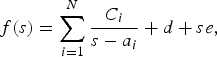
where d and e are optional real numbers, C i and a i are, respectively, the zeros and the poles, and s is the frequency.
The poles are identified by solving the following linear problem:
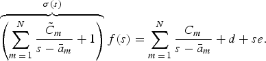
The unknowns of this equation (cm, d, e,  ) make it a linear one.
Applying (2) for several frequency samples give the over-determined linear problem,

where (cm, d, e,  ) are included in the solution vector x. Equation (3) is solved as a least squares problem.
Solving the linear problem (3) with accuracy needs a convenient choice of the starting poles to successfully apply the VF method. In order to achieve this, two conditions are required. The first one is to choose the starting poles in the complex form, because the linear problem becomes ill conditioned once real poles are chosen.
The other condition is to reduce the number of iterations required, by locating the starting poles in a sensitive location. However, this number is significantly related to the choice of the position of the starting poles.
This method is particularly suitable in the case of MIMO systems, for instance, a power combiner of a PA, which is commonly represented by its S matrix according to frequency.
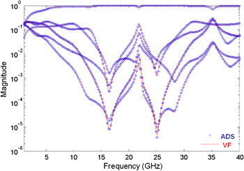
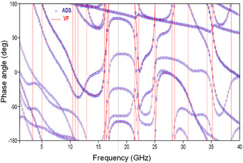
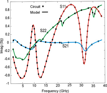
The following example assumes the power distributor issued from a two-stage X band PA. Figures 1 and 2 show, respectively, the accuracy of the magnitude and the phase of VF algorithm for modeling the full S matrix of this circuit from DC up to 40 GHz.
Magnitude of S-parameters versus frequency modeled by VF (X band PA's power distributor).

Phase of S-parameters versus frequency modeled by VF (X band PA's power distributor).

The rational identification of the complete S matrix is perfect if 40 poles are considered in the modeling process. If we reduce the bandwidth to that of the amplifier (i.e. 15%), 24 poles are sufficient.
VF is also a very robust method since the S-parameters are fitted using stable poles. Moreover, this method ensures the passivity enforcement (i.e. physical behavior of the resulting model entails that it should absorb active power for any set of applied voltages, at any frequency) which leads to a stable time-domain simulation.
III. SYSTEM-LEVEL IMPLEMENTATION, FOR CONTROL FLOW ENVELOP SIMULATION OF MIMO BLOCKS
Scilab is a CAD tool included in the scientific computing software ScicosLab [7]. It performs both, the modeling in the form of block diagrams and the simulation of hybrid dynamic systems including continuous- and discrete-time sub-systems; the input and output ports could be of two types: regular and activation.
Scicos uses explicit and implicit solvers for differential equations that allow the temporal integration of continuous nonlinear sub-systems. Scicos is an open simulation framework that includes a graphical editor for constructing models by interconnecting blocks, which permits the description of models in Modelica language.
Modelica language is an object-oriented, general-purpose language for modeling of physical systems, mechanical, electrical, and control systems [8]. The Modelica language allows a direct and convenient specification of systems with continuous-time and discrete-time dynamics.
The combination of Scilab/Scicos environment and Modelica language allows the modeling and time-domain simulation of bilateral sub-systems, which is the key point of the topological approach.
The associated Scicos block is written in Modelica, which allows us to define an implicit relationship between inputs and outputs; the same representation is used to associate each considered parameter S ij [Reference Mehdi, Bennadji, Mons, Ngoya and Quere9], hence the calculation of the following power wave equations (4)
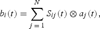
where ⊗ is the convolution operator.
Usual transformations between voltage/current and injected/reflected power waves are needed, assuming that a j are the inputs and b i the output at port i of the block.
A C-program is used to compute the Laplace transform representing the time-domain response using the following equation:
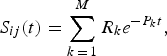
where R i and P i are, respectively, the residues and poles obtained by VF algorithm and M is the order of decomposition.
Each S ij contribution in equation (4) is computed by numerical convolution between the input power wave a j(t) and the S ij(t) impulse response. For CPU efficiency, the numerical convolution leads to compute a linear function that depends only on a i(t), t n (present time), and t n−1 (past time):

Hence, an efficient programmable form is obtained using the rectangle method for integral approximation:

where
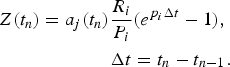
Also, equation (7) is effective for the numerical convolution computation (CPU efficiency) by keeping the results in a Z register to use them in the next step. Moreover, this approach is valid irrespective of the number of access of the block.
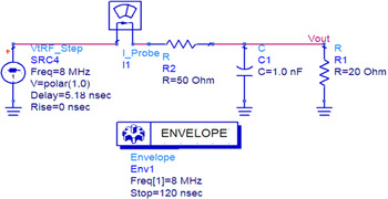
The first validation is realized on a very simple RC circuit, as shown in Fig. 3.
RC circuit envelope simulation (ADS).

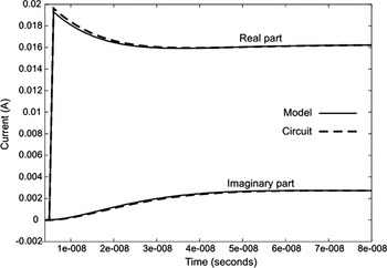
The comparison is made between circuit-level envelope simulation (ADS) and its system-level time-domain simulation (Scicos). Figure 4 shows the current response when the circuit is excited by a pulse signal.
Simulation-based behavioral model compared to circuit time response.

One can notice that the model is very perfect in this case if compared with envelope ADS simulation.
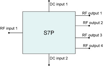
The second validation is realized on a much more complex circuit, the power distributor of the X band PA already defined by choosing the results of VF modeling in Figs 1 and 2 (Fig. 5).
X band power distributor (seven ports).

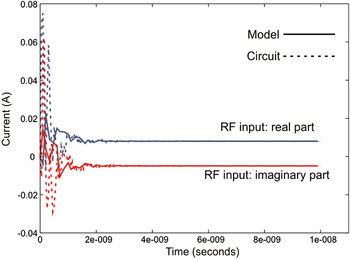
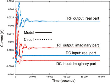
Figures 6 and 7 give a comparison between the model implemented in Scicos and the envelope simulation in ADS. Figure 6 presents the real (in blue) and imaginary (in red) parts of the input RF current, whereas Fig. 7 gives the RF output and the DC input currents.
Real and imaginary parts of the RF input current varying with time. Model response (solide line) compared to circuit one (dash line).

Real and imaginary parts of the RF output and the DC input currents varying with time. Model response (solid line) compared to circuit one (dash line).

A very good agreement between the model (simulated at the system level, i.e. Scicos) and the circuit (simulated at the circuit level, i.e. ADS) is observed in the steady state. However, a difference is noticed during the transient state (time less than 2 ns). This power distributor contains transmission lines and the ET simulation of ADS simulator encounters some difficulties in finding an accurate solution in the transition state. This transient response is not accurate and depends on the time step taken during the simulation.
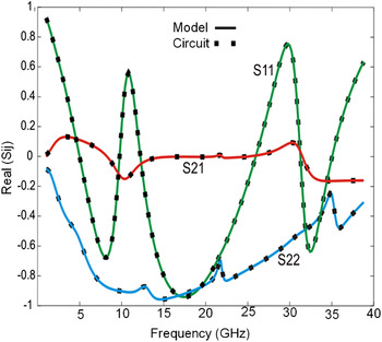
The power wave's a i and b i can be used at the system level for re-calculating the S-parameters. Figures 8 and 9 give a comparison between the S-parameters derived from a time-domain simulation at the system level (Scicos) with the original ones.
Real parts of the S-parameters re-calculated at the system level (solid line) compared to original ones (squares).

Imaginary parts of the S-parameters re-calculated at the system level (solid line) compared to original ones (squares).

Whereas the results of our approach are validated in the case of a localized circuit (Fig. 4), they can be considered as successful in this case. It is essential to mention that his approach is studied regardless of the presence or absence of transmission lines.
These results confirm that this behavioral approach is promising to evaluate the envelop response of a PA, submitted to a realistic signal, in a spice-like tool.
IV. CIRCUIT-LEVEL IMPLEMENTATION FOR ROBUST TRANSIENT ENVELOPE SIMULATION OF PA
In this part, an alternative to S-parameters models is given at the circuit level. This approach aims to improve the circuit simulation by generating an equivalent circuit that contains only simple lumped R, L, C components.
The generated equivalent circuit's simulation is simple; it circumvents the convergence problems made in the presence of actual signals, and overcomes the ET simulation's problem where the passive circuits contain transmission lines or EM-derived models.
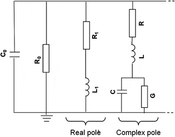
This method allows us to replace the linear sub-circuit (which contains transmission lines) by the synthesized one (R, L, C model). The model's implementation in the circuit CAD tool is performed using the synthesis circuit technique, after the calculation of the PR model by the VF method. The Matrix Fitting (MTRXFIT) method [Reference Gustavsen10] associates an R, L, C resonant circuit to each pole as presented in Fig. 10.
Admittance representation of the PR model.

The R, L, and C element values of this circuit are easily obtained using the following calculation method:


In the case of a real pole, the equivalent admittance has the following form:

where r i and p i are the residues and poles, respectively, then
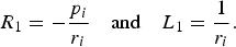
In the case of a complex pole, the equivalent admittance is calculated using the following form:
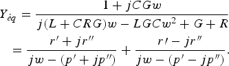
After the calculation of Y eq, we can calculate the R, L, and C components of the complex pole:




The synthesis circuit is based on an admittance representation, where all the branches are associated in a parallel form. Thus, an equivalent circuit for each Y ij parameter can be obtained.
The synthesis circuit implementation in a CAD environment is made automatically by generating a SPICE file, which is compatible with most circuit CAD tools.
A Matlab algorithm covers the entire process, starting from the poles/residues identification, to the equivalent circuit's synthesis, concluding by the circuit's implementation in a CAD environment.
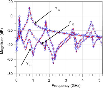
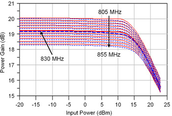
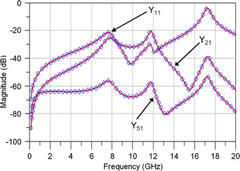
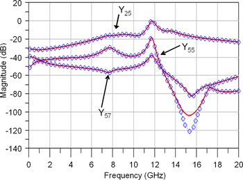
The first validation is realized on the passive circuits of a PA. This PA operates at 850 MHz and has a maximum gain of 19 dB. Since the passive parts contain only lumped components, ET simulation is very accurate. Figures 10 and 11 show the comparison of the circuit and the synthesized model on the Y-parameters. A very good agreement is observed on this three-port component.
Y-parameters (magnitude) versus frequency. Model (solid line) compared to circuit one (circles).

The synthesis process could now be applied to all the passive parts of the PA (power distributor and power combiner) to compare the efficiency of this approach on the full PA.
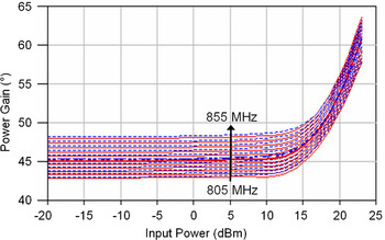
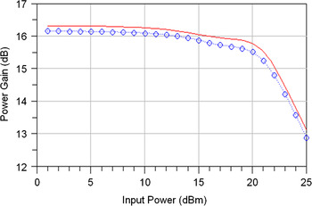
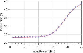
These circuits are evaluated in the case of a harmonic balance (HB) simulation. Figures 13 and 14 give the comparison of the gain in the case of PA when the passive parts are synthesized or not. These results are obtained by scanning the PA's frequency band, and varying the power generator's values from −20 to 22 dBm.
Figures 12 and 13 show the comparison results, a maximum error of 0.005 dB is observed between the circuit and the model. We can conclude that the synthesized circuit well represents the passive one. In fact, the HB simulation requires a very well accurate response of passive circuit in the frequency band of the PA, as well as in the DC simulation.
Y-parameters (magnitude) versus frequency. Model (solid line) compared to circuit (circles).

Power gain (magnitude) versus input power. Model (solid line) compared to circuit (dash line).

The final step is the validation of our approach in the case of ET simulation. A time-domain signal is applied to these two circuits. As shown in the preceding paragraphs (Figs 6 and 7), most ET simulations of the passive circuits containing transmission lines are not accurate.
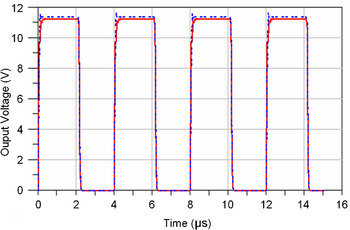
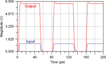
On the other hand, this PA contains only lumped elements, which allow us to precisely simulate this circuit and validate our approach by comparison with it. Figure 14 shows the comparison results when the circuit and its model are submitted to a pulse signal (Fig. 15).
Power gain (phase) versus input power. Model (solid line) compared to circuit (dash line).

Output voltage versus time. Model (solid line) compared to circuit (dash line).

After the validation of the synthesis process on a “small” PA which exhibits good convergence properties using ET (on radar or Telecom signal), we apply this technique on a complex PA where ET simulation is problematic.
For the second example given in predefined part (three-stage X band PA which operates at 10 GHz) we face consecutive problems: This PA operates with radar signals (time-domain discontinuities), all linear sub-circuits are derived from a MOMENTUM simulation (S-parameters defined from DC up to 40 GHz). In consequence, the number of harmonics must be smaller than 4, which is not enough in this case. No convergence is observed while performing ET simulation in this case. This method is now applied to all their passive parts.
Figure 16 shows the comparison of some Y-parameters after the synthesis process.
Y-parameters (magnitude) versus frequency. Model (solid line) compared to circuit one (circles).

A good accuracy is observed on the PA's frequency bandwidth.
These results allow us to test the HB simulation of the PA using the synthesized circuits. Figure 17 shows the validation of this simulation by comparing the gain of the PA in these two cases (Figs 18 and 19).
Y-parameters (magnitude) versus frequency. Model (solid line) compared to circuit one (circles).

Power gain (magnitude) versus input power. Model (solid line) compared to circuit (dash line).

Power gain (phase) versus input power. Model (solid line) compared to circuit (dash line).

The maximum error that is observed is about 0.15 dB. Finally, the PA's model is submitted to a pulse signal using ET simulation. Figure 20 shows the input and output voltage results of the PA.
Input and output voltages versus time.

These results could not be compared since this PA was not converged in the ET simulation, but according to the ET results of the simple PA (Figs 13 and 14) and to the HB and S-parameters results of this X band PA (Figs 15–17), we demonstrate that this approach is useful to circumvent the convergence problems while using ET simulation. It gives an alternative way for the prediction of performances on complex circuits if troubleshooting during ET simulation is observed.
V. CONCLUSION
The circuit envelope analysis that is used in ADS from Agilent allows simulating circuits with realistic signals. This method seems highly efficient in analyzing circuits with digitally modulated signals, because the transient simulation takes place only around the carrier and its harmonics. A consequence of this method is that any components that are characterized in the frequency domain need to have their response converted to the time domain for the portions of their frequency response which fall within the envelope bandwidth. In the case of complex circuits such as PAs, the ET simulation is still problematic if transmission lines or S-parameters are used. Using VF method seems to be a particular effective solution for the representation of MIMO blocks. In this paper, we firstly presented a time-domain implementation of S matrices at the system level, regardless of the value of the access number N. Thus, efficient bilateral implementation of passive circuits – such as filters, circulators – is now possible. This approach was validated in the system CAD tool in the cases of simple and complex circuits. Moreover, VF is effective in the case of ET simulation, regardless of the complexity of the used passive circuit. This approach provides a solution if transmission lines or [S] parameters files are used, by generating an equivalent circuit containing only lumped components. This approach was validated in ADS on PAs using HB and ET simulations and provides a solution if ET does not converge. The next step will be the implementation of a full topological model of HPA in a system environment simulation, where the passive parts and the active parts will be, respectively, represented by a VF approach and a nonlinear scattering function [Reference Estagerie, Bennadji, Reveyrand, Mons, Quéré and Constancias4].
 Hassan Mehdi was born in Saida Lebanon in 1983. He received the Ph.D. degree from the University of Limoges, Limoges, France, in 2010. His main research interests include passive circuit and power amplifiers modelling.
 Sébastien MONS was born in Limoges (France) in 1970. He received the Ph.D. Degree in Electronics from the University of Limoges in 1999. He joined the Microwave Laboratory of the CNES of Toulouse, France, in 1999. Since October 2001, he is a researcher of the French CNRS at XLIM institute, Limoges University. His main research interests include system level modelling and nonlinear analysis of microwaves circuits.
 Edouard NGoya received the Ph.D. degree in electronics from the University of Limoges, Limoges, France, in 1988. In 1990, he joined the French Centre National de la Recherche Scientifique (CNRS), XLIM (formerly IRCOM laboratory). He is the inventor of key analogue simulation and modelling technologies such as compressed transient, ET, and dynamic Volterra series. Since 1998, he has been the Consultant Chief Scientist with Xpedion Design Systems, Milpitas, CA. His current research activities focus on modelling and simulation techniques for large-scale integration RF circuits, RF system-on-chip (SOC) and system-in-package (SIP).
 Abderrazak Bennadji was born in Chlef, Algeria, in 1975. He received the Electronic engineering Degree from University of Blida, Algeria, in 1999, the Phd degree in electronic from the University of Limoges. From 2006, he works in institute of microwave and optical communications, University of Limoges, where he is currently involved with modeling and implementation of the amplifier models in the system simulators.
 Raymond Quéré (Fellow IEEE) was born in 1954 in St Brieuc (France). He received the Electrical Engineering degree from ENSEEIHT Toulouse, France in 1976. He prepared and earned a Ph.D. degree from University of Limoges in 1989. In 1992, he was appointed full professor at the University of Limoges. From 1992 to 1997 he headed the Department of Electrical Engineering at the Institute of Technology of the University of Limoges. Since 1998 he leads the Nonlinear High-frequency Devices, Circuits and Systems Research Department at XLIM-CNRS Laboratory. His main field of interest is in the area of nonlinear device and circuit modelling with a particular emphasis on nonlinear phenomena such as stability in power amplifiers.