1. Introduction
The growing urgency of addressing climate change has brought to light the intricate connections between economic growth, environmental sustainability, and fiscal policies (see, for instance, Besley and Persson (Reference Besley and Persson2023), Catalano et al. (Reference Catalano, Forni and Pezzolla2020), Jaimes (Reference Jaimes2023)). As governments worldwide seek to balance these competing objectives, understanding the dynamics that govern this relationship has become a critical area of research. Climate change poses significant risks to both economic output and environmental quality, and the role of policy intervention in mitigating these risks is paramount. This paper aims to contribute to this ongoing discourse by developing a dynamic overlapping generations (OLG) model incorporating pollution as a direct by-product of economic production, linking economic activity to environmental degradation.
Building on the works of John and Pecchenino (Reference John and Pecchenino1994), Antoci and Sodini (Reference Antoci and Sodini2009), Fodha and Seegmuller (Reference Fodha and Seegmuller2012), Wei and Aadland (Reference Wei and Aadland2022), Dávila-Fernández et al. (Reference Dávila-Fernández, Giombini and Sánchez-Carrera2023), Caravaggio and Sodini (Reference Caravaggio and Sodini2023), and Jaimes (Reference Jaimes2023), we analyze an environmental OLG framework by modeling pollution damage as a function of pollution, which is driven by economic output. This allows us to extend the previous works and get a more direct and simplified representation of how economic growth influences environmental outcomes, capturing the feedback loops between production, pollution, and fiscal policy. Our model introduces government fiscal policy through government spending financed by taxation and public debt, reflecting the real-world dynamics in which fiscal measures play a crucial role in shaping economic and environmental outcomes.
Several contributions have quite recently studied the interplay between production, pollution and public debt (see among the others Fodha and Seegmuller (Reference Fodha and Seegmuller2014), Catalano et al. (Reference Catalano, Forni and Pezzolla2020), Boly et al. (Reference Boly, Combes, Menuet, Minea, Motel and Villieu2022)). In contrast to this literature, we investigate and compare the long-term equilibrium behavior of economies under varying levels of government intervention. By examining the interaction between initial economic conditions (capital and pollution levels), government policies, and individual preferences for environmental quality, we aim to understand how different policy regimes influence the trajectory of economic and environmental variables.
This paper makes several key contributions to the literature. First, it provides a more comprehensive view of the fiscal implications of climate change in presence of private mitigation. Second, it explores the role of individual preferences for environmental quality in shaping long-term outcomes, particularly in pollution dynamics. Finally, the model offers nuanced insights into the trade-offs between economic growth and environmental sustainability under varying government interventions. Our findings underscore the role of multistability in shaping economic and environmental trajectories, where different equilibrium states emerge depending on initial conditions and the degree of government intervention. The existence of multiple equilibria implies that even minor initial variations can lead to markedly different long-term outcomes, reinforcing the idea that economic development is highly path-dependent. Maybe closely related to the well-known environmental Kuznets curve (Dinda, Reference Dinda2005; Ridzuan, Reference Ridzuan2019), which posits the existence of an inverted U-shape relationship between environmental degradation and economic development.
While our dynamic model is non-linear, their results do not support the environmental Kuznets curve hypothesis (in line with the empirical evidence pointed out by Özokcu and Özlem Özdemir (Reference Özokcu and Özdemir2017) and Wang et al. (Reference Wang, Li and Li2024)). Since, we show that limited government intervention, characterized by low taxes and reduced public spending, can help prevent capital erosion and severe environmental degradation. When government intervention is minimal or moderate, the system exhibits branching dynamics, where economies that begin with low levels of capital and pollution may follow a self-reinforcing trajectory toward sustained capital accumulation and environmental stability. Conversely, those economies starting with high capital and pollution risk settling into an equilibrium where pollution remains persistently high while capital levels decline. This pattern underscores the need for early policy action. Once pollution exceeds a certain threshold, the mechanisms that would otherwise support capital accumulation and ecological recovery weaken significantly, as environmental degradation cannot be resolved automatically through economic growth. Consequently, economies burdened by high initial pollution may find it difficult to escape the low-capital, high-pollution trap without timely intervention. On the other hand, strong government intervention can counteract some of the effects of initial disparities by directly fostering capital accumulation. However, this approach often leads to higher pollution levels, revealing an inherent trade-off between economic growth and environmental sustainability. Our calibration results highlight the reinforcing link between excessive pollution and economic decline. Without corrective measures, the destructive effects of pollution on capital formation could become self-perpetuating, leading to prolonged economic stagnation.
The rest of the paper is organized as follows. Section 2 presents our OLG model with a detailed explanation of its main transmission channels, yielding an economy composed of a dynamic system representing the government, households, and firms. Section 3 provides the main dynamic properties of such an economic system. Section 4 studies the main numerical scenarios, while subsection 4.2 presents the results on the policy implications for characterizing equilibrium economies. Subsection 4.3 presents a country-specific calibration analysis. Section 5 offers some final considerations.
2. The model
We examine a dynamic general equilibrium model with pollution and a government issuing public debt. Time is discrete,
 $t\in \mathbb{N}$
, and population is constant. Pollution affects the economy through a damage function reducing production. On the consumption side, we consider an OLG economy where individuals live two periods: youth and old age. In the first one, they work and save all their earnings by investing in capital or government bonds. They can also use their wage to improve environmental conditions. During the second period, they utilize their accumulated savings for consumption.
The first original and key ingredient of our approach lies in modeling the damage function
 $D(\cdot)$
. In our case, it is a function of pollution influenced by economic production. This approach simplifies the complex interactions by establishing a direct link between economic activity and changes in pollution levels, thus providing a more straightforward representation of the impact of economic growth on global warming.
Secondly, our analysis uses government budget constraints including public debt and taxation of the polluters. Hence, our analysis introduces a tax revenue function to assess climate change’s fiscal implications more comprehensively. The primary motivation for this inclusion is to reflect the real-world economic dynamics where government fiscal policy plays a crucial role in influencing economic stability and growth. Tax revenue is derived as a fraction of the output in our model. This approach allows us to capture the dual effect of climate change on both economic output and government fiscal capacity as it models the diminishing returns to tax revenue in the face of increasing pollution, thereby providing a more nuanced understanding of the economic impacts of climate change. By integrating taxation into our model, we aim to offer a more holistic view of the economic and fiscal dynamics under varying climatic conditions. This modification aligns with the broader literature that emphasizes the interplay between economic decisions and environmental quality in OLG models (John and Pecchenino Reference John and Pecchenino1994; de la Croix and Gosseries Reference de la Croix and Gosseries2012).
2.1 Production, pollution and damage function
Firms use a production technology that integrates capital (
 $K\gt 0$
) and labor (
 $N\gt 0$
), with labor representing a constant number of workers. Pollution acts as a detrimental externality on production factors. It impacts the capital stock directly through natural disasters or indirectly by heightening the fear of potential extreme events, thereby decreasing profitability. Production follows as:
 \begin{equation*} Y_t=\frac {1}{1+D(P_t)}F(K_t,N_t) \end{equation*}
where
 $D^\prime (P)\gt 0$
, and
 $F(K_t,N_t)$
is an increasing function with respect to capital and labor, concave and homogeneous of degree one.
 $Y_t\gt 0$
denotes output, and
 $P_t\in {\mathbb{R}^+}$
the level of pollution, and
 $1/(1+D(P_t))$
the proportion of economic output lost due to climate change. Consequently, higher emissions result in higher pollution and environmental degradation, which in turn reduces overall output. In the following, we normalize the number of workers, i.e.
 $N=1$
. Therefore, the output is given by:
 \begin{equation} Y_t=\frac {F(K_t,1)}{1+D(P_t)}. \end{equation}
In our analysis, we specify the damage function as initially proposed by Nordhaus (Reference Nordhaus1991), which has been a foundation for much of the recent literature. In the Dynamic Integrated Climate and Economics (DICE) model, Nordhaus (Reference Nordhaus2008) assumes that damages can be well-approximated by a quadratic function of temperature, while Bretschger and Vinogradova (Reference Bretschger and Vinogradova2018) discusses the linear relation between temperature and pollution. Following these arguments, we consider:
 \begin{equation} D(P_t)=\rho P_t^2, \quad \rho \in [0,1] \end{equation}
We use a simple pollution dynamics model that directly links economic production to pollution change: we assume that
 $Y_t$
directly impacts future pollution
 $P_{t+1}$
, but private mitigation
 $n_t$
may reduce the pollution flows:
 \begin{equation} P_{t+1} =(1-\delta) P_t + \lambda Y_t -\eta n_t \end{equation}
where
 $\lambda \gt 0$
measures the sensitivity of pollution to production changes,
 $\eta \gt 0$
the efficiency of mitigation,
 $n_t$
. At the same time,
 $\delta \in [0,1]$
is the decay rate of pollution, i.e. represents the rate at which pollutants inherited from the past
 $P_t$
dissipate.Footnote
1
Thus, production and mitigation at period
 $t$
directly affect the future stock of pollution
 $P_{t+1}$
, which is a negative externality on future production and income.
To simplify the analysis, we use a Cobb–Douglas production function:
 \begin{equation*} F(K_t,1)=AK^\alpha _t \end{equation*}
where
 $\alpha \in (0,1)$
represents the capital share in income, while
 $A\gt 0$
serves as a scaling parameter reflecting total factor productivity.
Production faces a proportional tax, at rate
 $\tau \in [0,1)$
. Therefore, profits are given by
 $(1-\tau)Y_t-w_tN_t-r_tK_t$
, where
 $w_t$
is the wage and
 $r_t$
the interest rate. Since there is perfect competition and
 $N_t=1$
, the firm’s profit maximization problem yields the following equations for wage and interest rates respectively:
 \begin{eqnarray*} w_t&=&\frac {1}{1+D(P_t)}(1-\tau)(1-\alpha)AK^\alpha _t \\ r_t&=&\frac {1}{1+D(P_t)}(1-\tau)\alpha AK^{\alpha -1}_t \end{eqnarray*}
The damage function introduces environmental degradation caused by emissions, which leads to decreased compensation for both production factors.
2.2 The government
Our analysis adopts a government budget constraint commonly found in macroeconomic literature. The standard government budget constraint can be expressed as follows:
 \begin{equation} B_{t+1} = (1 + i_t)B_t + G_t - T_t \end{equation}
where
 $ B_{t+1}$
represents the government debt at time
 $ t+1$
,
 $ i_t$
the interest rate which remunerates debt holding,
 $ G_t$
denotes government spending, and
 $ T_t$
tax revenue.
To integrate the impact of climate change on tax revenue, we propose an equation incorporating a feedback mechanism reflecting the adverse effects of increased pollution on economic productivity.Footnote
2
The tax revenue
 $ T_t$
is modeled as a proportional tax on production with rate
 $\tau \in [0,1)$
. The tax revenue equation is given by:
 \begin{equation} T_t=\tau Y_t\,. \end{equation}
This formulation captures the dual impact of climate change on economic performance and fiscal capacity, providing a comprehensive view of the fiscal dynamics under varying climatic conditions.
We represent government spending
 $ G_t$
as a share of GDP to align with the extensive body of literature underlying the interplay between fiscal policy and economic growth, i.e.
 \begin{equation} G_t = \psi Y_t \end{equation}
where
 $ \psi \in (0,1)$
represents the proportion of GDP allocated to government spending.Footnote
3
Using the above mentioned equation, our model captures an essential interaction between government spending and economic output, which conveys the idea that an important policy parameter corresponds to the level of public spending over GDP.
The two fiscal instruments are the tax rate
 $\tau$
and government spending over GDP
 $\psi$
. The first is a tax on polluting activities paid by the polluters, i.e., the firms, on production. An increase in this tax will hurt production, reducing pollution flows. For the second one, note that public spending is a share of aggregate demand, rather than an expense, that directly reduces the effect of pollution flows. Any increase in public spending will raise public debt, and, as we will see in the next section, public debt is part of a household’s savings. Therefore, higher public debt will have a crowding-out effect on capital investment, reducing future production and future pollution flows. Through this channel, government spending affects pollution.
2.3 Households and lifetime choice
Household members live in two periods and derive utility from consumption,
 $c_{t+1}$
, and pollution levels,
 $P_{t+1}$
. When the member is old, the utility function is:
 \begin{equation} U(c_{t+1}, P_{t+1}) = \ln c_{t+1} - \epsilon \ln P_{t+1}, \end{equation}
where
 $\epsilon \gt 0$
is a measure of green preferences. Note that the specification of the utility function,
 $U(c_{t+1}, P_{t+1}) = \ln c_{t+1} - \epsilon \ln P_{t+1}$
, is already used in Balleer and Endrikat (Reference Balleer and Endrikat2023) and it allows to avoid too complicated computations. It is, however, important to note that when
 $P_{t+1}$
varies, it modifies the disutility for pollution but the utility for consumption, too, because consumption is lower than production given by Eq. (1). For instance, if pollution increases and tends to infinity, the marginal disutility of pollution decreases. Still, consumption will tend to be zero, meaning pollution’s total marginal utility will not be zero.
In the first period, the household’s member earns a labor income equal to the wage because of an inelastic labor supply normalized to one. Income’s share goes to a portfolio choice between investing in the capital used in the production at the next period,
 $K_{t+1}$
, financing public debt issued by the government at the end of period
 $t$
,
 $B_{t+1}$
, and environmental mitigation,
 $n_t$
. In the second period, capital remuneration is at the interest factor
 $r_{t+1}$
under a complete depreciation of capital, and public debt is remunerated at the interest factor
 $1+i_{t+1}$
according to the inter-temporal budget constraint of the government, Eq. (4). Indeed, by convention, it is assumed that the public debt financed by young households’ members at period
 $t$
, denoted by
 $B_{t+1}$
and, as usual, the interest paid by the government at period
 $t+1$
is
 $i_{t+1}$
.Footnote
4
Therefore, a household maximizes its utility under the following constraints:
 \begin{eqnarray} w_t &=& K_{t+1} +B_{t+1} + n_t \end{eqnarray}
 \begin{eqnarray} c_{t+1} &=& r_{t+1}K_{t+1} + (1+i_{t+1})B_{t+1} \end{eqnarray}
and Eq. (3). The first constraint indicates that young agents’ wage income must be allocated among capital savings, government bonds, and resources dedicated to mitigation measures (
 $n_t$
). The second constraint shows that older agents’ consumption (
 $c_{t+1}$
) is financed by their youth’s remunerated savings, which include capital and government bonds. Finally, Eq. (3) implies that households opt for environmental mitigation to attenuate the intergenerational impact of pollution on their well-being.
Note that the two assets
 $K_{t+1}$
and
 $B_{t+1}$
are perfect substitutes. This implies that:
 \begin{equation*} r_{t+1}=1+i_{t+1}=\frac {(1-t)\alpha AK^{\alpha -1}_t}{1+D(P_t)}\,. \end{equation*}
Hence, a household member needs to solve:
 \begin{equation} \max _{n_t} \ln \left (r_{t+1} (w_t - n_t) \right) - \epsilon \ln \left [(1-\delta)P_t + \lambda Y_t - \eta n_t\right ] \end{equation}
subject to
 $n_t\geq 0$
. We deduce that:
 \begin{equation} \frac {r_{t+1}}{c_{t+1}}\geq \frac {\epsilon \eta }{P_{t+1}} \end{equation}
with an equality when
 $n_{t}\gt 0$
. Solving this optimization problem provides the optimal allocation between consumption and mitigation efforts, balancing the immediate utility of consumption with the long-term benefits of reduced pollution.
3. Existence of long-run equilibria
This section examines the conditions under which inter-temporal equilibria are feasible. A critical first step is determining the range of achievable values for
 $n_t$
; the resources individuals allocate to pollution mitigation. Specifically, the value of
 $n_t$
must satisfy two constraints: Firstly,
 $n_t$
cannot exceed the individual’s earnings,
 $w_t$
. This is because individuals cannot allocate more resources to pollution mitigation than they generate from their wages. Thus, the upper bound for
 $n_t$
is inherently limited by
 $w_t$
. Secondly, a practical maximum exists for
 $n_t$
, beyond which further investment in pollution mitigation would be inefficient. Specifically,
 $n_t$
should not exceed the level that would eliminate pollution
 $P_{t+1}$
, as it would be wasteful for individuals to dedicate more resources than necessary to achieve zero pollution. Investing beyond this threshold would result in diminishing returns, offering no additional environmental benefit. Therefore, the optimal upper bound for
 $n_t$
is determined by the pollution level at which further mitigation yields no additional reduction in pollution levels. These considerations are summarized in the following assumption:
Assumption 1. Resources allocated to pollution mitigation are limited by an individual’s wage and the level of resources required to mitigate pollution fully. Therefore:
 \begin{equation*} n_t\le n_{max}, \quad n_{max}=\min (w_t,n^{(p)}) \end{equation*}
where
 \begin{equation*} n^{(p)}=\frac {(1-\delta)P_t+\lambda Y_t}{\eta }. \end{equation*}
These constraints provide the foundation for the subsequent analysis of equilibria in the system, as they help delineate the feasible space within which individuals’ decisions can interact with environmental and economic dynamics. The second step is to determine which values of
 $n_t$
maximize the utility function of the households. Given that individuals derive utility from consumption and pollution mitigation, finding the optimal allocation of resources to these competing needs is crucial. Let us present a proposition that addresses this optimization problem and identifies the values of
 $n$
that maximize household utility (Proof in Appendix A.1).
Proposition 1.
Let the maximization problem of the households be given by (
10
) and assume
 $\lambda _1\equiv \eta (1-\tau)(1-\alpha)$
,
 $n^*=\frac {N_t+(\lambda -\epsilon \lambda _1)M_t}{1-\epsilon }$
. Then
-
• In case
 $\epsilon \gt 1$
and
-
–
$\lambda _1\lt \lambda \lt \epsilon \lambda _1$
and
$P_t\lt P^{(\epsilon)}$
-
–
$\lambda \lt \lambda _1$
and
$P^{(\lambda)}\lt P_t\lt P^{(\epsilon)}$
the optimal level of
$n_t$
is
$n^*$
; -
-
• In case
$\lambda \lt \lambda _1$
and
$P_t\lt P^{(\lambda)}$
, the optimal level of
$n_t$
is
$n^{(p)}$
; -
• In all other cases the optimal level of
$n_t$
is zero;





where
 $N_t=\frac {(1-\delta)P_t}{\eta }$
,
 $M_t=\frac {AK_t^\alpha }{\eta \left (1+\rho P_t^2\right)}$
and
 $P^{\epsilon },P^{\lambda }$
are given in Appendix A.1
.
Since we have established the households’ decision regarding
 $n_t$
(the resources allocated to pollution mitigation), we can proceed by analyzing the overall dynamic system. This system is governed by the evolution of three key variables: pollution, government debt, and capital stock. Each variable follows its dynamic equation, reflecting economic production, environmental conditions, and fiscal policy interactions. The resulting dynamical system is:
 \begin{align} K_{t+1} & = w_t-B_{t+1}-n_t\nonumber \\ B_{t+1} & = r_tB_t+(\psi -\tau)Y_t \\ P_{t+1} & = (1-\delta)P_t + \lambda Y_t - \eta n_t \nonumber \end{align}
Note that the first equation corresponds to the household’s budget constraint at the first period of life (8), where savings are for investing in capital and buying new public debt at equilibrium. The second equation is the inter-temporal budget constraint of the government in which we substitute the expressions of government spending (6) and tax revenue (5). The third equation corresponds to the evolution of the pollution stock, given by (3).
First, we will focus on analyzing the system’s equilibria. A fixed point represents a state where the system remains unchanged over time, meaning that once it reaches this state, it will stay there unless perturbed. For system (12) the following proposition holds (proof in Appendix A.2):
Proposition 2.
Considering that
 $n=n^*$
, then:
-
• In case
$\epsilon \delta \gt 1\wedge \lambda \gt \lambda _1$
or
$\epsilon \delta \lt 1\wedge \lambda \lt \lambda _1$
, there exist the fixed points
$E^{*}$
,
$E^{*1}$
and
$E^{*2}$
(defined in Appendix A.2),
-
– if
$r\gt 1 \wedge \psi \lt \tau$
or
$r\lt 1 \wedge \psi \gt \tau$
a unique fixed point exists given by
$E^*\equiv (K^*, B^*, P^*)$
-
– if
$r\gt 1 \wedge \psi \gt \tau$
or
$r\lt 1 \wedge \psi \lt \tau$
up to two fixed points may exist given by
$E^{*1}\equiv (K^{*1}, B^{*1}, P^{*1})$
and
$E^{*2}\equiv (K^{*2}, B^{*2}, P^{*2})$
-
-
• Otherwise, no fixed point exists.









When individuals decide to invest a portion
 $n^*$
of their resources in improving the environment, this does not automatically result in equilibrium in the economy. For one or two equilibria to emerge, one of two conditions must be satisfied, i.e., either individuals derive little utility from the environment (with
 $\epsilon \lt 1 / \delta$
, but not much more) and the damage caused by production is low (
 $\lambda$
is sufficiently low), or individuals derive significant utility from the environment (
 $\epsilon \gt 1/ \delta$
), and the damage from production is substantial (
 $\lambda \in (\lambda _1, \epsilon \lambda _1)$
). In intermediate cases, where either interest in the environment is high but the damage is low, or damage is great but interest is low, no equilibrium points arise in the economy shaped by pollution, capital, and government.
We now turn to the final case: When individuals derive little benefit from the environment, or even if they derive significant benefit, but the damage caused by production is very high, they choose not to allocate resources toward environmental protection. The consequences of this decision, in terms of equilibria, are captured in the following proposition (Proof in Appendix A.3).
Proposition 3.
Consider the case in which
 $n=0$
.
-
• In case
$\epsilon \gt 1 \wedge \lambda \ge \delta \epsilon \lambda _1$
or
$\epsilon \lt 1 \wedge \lambda \ge \delta \lambda _1$
there exist fixed points
$E^{\dagger }$
,
$E^{\dagger 1}$
and
$E^{\dagger 2}$
(defined in Appendix A.3),
Footnote
5
-
– if
$r\gt 1 \wedge \psi \lt \tau$
or
$r\lt 1 \wedge \psi \gt \tau$
a unique fixed point exists given by
$E^\dagger \equiv (K^\dagger, B^\dagger, P^\dagger)$
-
– if
$r\gt 1 \wedge \psi \gt \tau$
or
$r\lt 1 \wedge \psi \lt \tau$
up to two fixed points may exist given by
$E^{\dagger 1}\equiv (K^{\dagger 1}, B^{\dagger 1}, P^{\dagger 1})$
and
$E^{\dagger 2}\equiv (K^{\dagger 2}, B^{\dagger 2}, P^{\dagger 2})$
-
-
• Otherwise, no fixed point exists.









When individuals do not invest in the environment, no equilibria are generated if the damage caused by production is not extremely high. However, for higher values of
 $\lambda$
, one or two equilibria can emerge. The number of these equilibria also depends on the interest rates of capital and government bonds, which influence how resources are allocated within the economy.
4. Dynamics and convergence: the numerical analysis
We have shown that the decision by individuals to allocate a portion
 $n^*$
of their resources toward environmental improvements does not inherently lead to an equilibrium in the economy. This result stems from the complex interplay between the utility individuals derive from the environment (
 $\epsilon$
) and the damage caused by production (
 $\lambda$
). For equilibrium to exist, there must be a balance between environmental concerns and the harm caused by economic activities. Specifically, two cases allow for such an equilibrium:
-
• Low environmental utility and low damage: When individuals gain little utility from the environment (
$\epsilon$
is greater than a threshold but not much larger than
$ 1 /\delta$
), combined with the low effect of production on pollution (
$\lambda$
is sufficiently low), an equilibrium can emerge. In this case, the individuals’ investment in environmental protection is limited, and the economy can adjust without significant disruptions. -
• High environmental utility and high damage: Alternatively, if individuals derive substantial utility from the environment (
$\epsilon \gt 1 /\delta$
) and the effect of production on pollution is significant (
$\lambda \in (\lambda _1, \epsilon \lambda _1)$
), such an equilibrium is also possible. Here, the strong desire for environmental protection incentivizes sufficient investment to counterbalance the larger damage caused by production.


However, in intermediate cases—where individuals have high environmental interest but production damage is low, or where production damage is high, but the environmental preference is low—no stationary equilibrium with
 $n^*$
is reached. This is because the misalignment between the costs and benefits of environmental investment prevents the economy from stabilizing. For instance, if individuals care deeply about the environment but the damage from production is minimal, their investment might overshoot what is necessary, leading to inefficiencies. Similarly, if production damage is high but individuals derive little utility from the environment, the investment in environmental protection is insufficient to offset the economic and environmental impacts. This outcome highlights the delicate balance between environmental concern and the economic costs of pollution and production, showing that equilibrium is only guaranteed with a specific alignment of these factors.
Lastly, when individuals choose not to invest in environmental protection, the system’s behavior heavily depends on the damage caused by production. When the damage caused by production is sufficiently high (i.e.,
 $\lambda$
is large), one or even two equilibria can emerge. This is because greater environmental damage creates stronger incentives for the system to adjust in ways that balance the economic consequences of production and capital allocation. The economy seeks stationary points where the interplay between environmental degradation and resource allocation can be resolved, often leading to multiple possible equilibrium points. The exact number of equilibria—whether zero, one, or two—depends on the damage caused by production and factors such as the interest rates on capital and especially the level of public debt.
The system’s global dynamics analysis indicates that, over time, individuals may adjust the amount of resources they allocate to environmental protection based on the pollution levels they observe. This evolving investment strategy means feedback loops between pollution, production, and resource allocation characterize the system. Therefore, it is not enough to identify the fixed points; one must also consider how the system moves around them and whether these points are attractive or repellent. Given the complexity of this system, where multiple interacting factors shape the outcomes, we will undertake this stability analysis in the following section using numerical simulations. Simulations allow us to understand the complete dynamics of the system and provide a complete understanding of the behavior of the fixed points.Footnote 6
4.1 Numerical analysis
As we proceed with the simulations, we will hold specific parameters at their baseline values while varying others to explore their impact on the system’s stability.Footnote 7
Specifically, natural environmental processes largely determine the decay rate of pollution
 $\delta$
, which is assumed to be a fraction between 0 and 1, indicating how fast pollution decays over time. In the study by Brausmann and Bretschger (Reference Brausmann and Bretschger2024), this value represents the rate at which excess pollutants dissipate from the environment. A common assumption is slow decay, with values like 0.01–0.5 depending on the nature of the pollutant and environmental absorption capacity; we set
 $\delta =0.15$
. The scaling parameter
 $A$
reflects the overall efficiency of the production process. It is commonly set based on empirical estimates of productivity in macroeconomic models. Values of
 $A$
are often normalized to 1 in theoretical models for simplicity but can range between 0.8 and 1.5 depending on the economy’s productivity (as suggested in growth literature). We set
 $A=1$
. Typically
 $\alpha$
is between
 $0.2$
and
 $0.4$
. We set
 $\alpha =0.3$
. In environmental models like those of Nordhaus (Reference Nordhaus1991),
 $\eta$
measures how effectively resources reduce pollution. This parameter is usually a fraction between 0 and 1, with higher values indicating more effective mitigation efforts. In several models,
 $\eta$
ranges from 0.2 to 0.8, depending on the context of pollution reduction technologies and policies. For the baseline value, we set
 $\eta =0.5$
. The parameter
 $\rho$
quantifies how sensitive economic output is to changes in pollution. In models such as the DICE model by Nordhaus (Reference Nordhaus2008),
 $\rho$
is assumed to be small but significant, typically between 0.001 and 0.1. This reflects the gradual but impactful reduction in output due to increasing pollution. We set
 $\rho =0.05$
.
In our simulations, we use three sets of values to represent different government policy approaches for the parameters
 $\psi$
(government spending as a share of GDP) and
 $\tau$
(tax rate). First is a low-intervention policy with
 $\psi = 0.15$
and
 $\tau = 0.2$
, where the government plays a minimal economic role. Second, a moderate-intervention policy with
 $\psi = 0.3$
and
 $\tau = 0.25$
reflects a balanced approach where government spending and taxation are moderate. Finally, a high-intervention policy with
 $\psi = 0.45$
and
 $\tau = 0.4$
represents a scenario where the government actively intervenes in the economy through higher spending and taxation. These different policies allow us to observe how varying levels of government involvement affect economic stability and growth in the presence of climate shocks.
As a first step in our analysis, we focus on examining the long-term dynamics of the system. The primary goal is to determine whether, over time, the system converges to a fixed point, enters a cycle (we explored cycles ranging from cycle-2 to cycle-100), or exhibits divergent behavior. We also examine the impact of varying levels of government intervention: Low, moderate, and high (as described previously). Then, we test the system’s long-term behavior starting from different initial conditions, mainly focusing on the state variables’ low, medium, and high values
 $K$
,
 $B$
, and
 $P$
. This allowed us to capture a broad range of initial economic conditions, from undercapitalized economies to those with substantial resources. Once these scenarios are present, we analyze the system’s long-term trajectory by focusing on the final 100 iterations after allowing for an 1100-iteration transitory phase. Thus, we vary the key parameters
 $\lambda$
(representing the damage caused by production) and
 $\epsilon$
(representing the utility individuals derive from the environment) across broad ranges. Specifically, we test the values of
 $\lambda$
between 0 and 1 and
 $\epsilon$
between 0 and 3 to observe how these parameters influence the system’s behavior.
As summarized in Table 1, in all considered scenarios, regardless of the type of economy or the level of government intervention, the system converges to a fixed point. This result holds for all combinations of initial conditions, values of the parameters
 $\lambda$
and
 $\epsilon$
, and the various evaluated levels of capital, bonds, and pollution. We can conclude that, regardless of the specific values of the variables, the system eventually stabilizes and reaches a long-run equilibrium.
Summary of long-term dynamics analysis across different government interventions

However, this analysis does not explicitly examine whether the equilibrium point is always the same across different scenarios or whether the system converges to different fixed points depending on the initial conditions or parameter settings. While convergence is guaranteed, multiple distinct equilibria remain open, and further analysis is required to determine whether the fixed points are identical or vary across different parameter spaces. It is crucial to understand which specific fixed point the system converges to. This is particularly important for determining the long-term dynamics of the economy. To address this, we investigate the equilibrium values of
 $K$
,
 $P$
, and
 $B$
across different scenarios of the key variables. The results for these equilibrium values are presented both graphically and through a set of detailed statistics. Given the extensive nature of this analysis, we have included the full results in Appendix B and will discuss them in depth in the next section.
4.2 Characterizing economies in equilibrium
The results obtained thus far have laid a solid foundation for understanding the existence of fixed point equilibria in our model. We have demonstrated that the decision to invest in environmental protection does not inherently guarantee the emergence of an equilibrium in the economy. Instead, equilibrium occurs only under specific conditions related to the balance between the utility derived from the environment and the damage caused by production. We explored various scenarios to determine whether the system converges to a fixed point equilibrium, enters a cyclical pattern, or diverges over time. The system consistently converged to a fixed point equilibrium across all scenarios—encompassing varying levels of government intervention and diverse initial conditions. However, this result alone is insufficient for fully understanding the system’s dynamics.
While establishing equilibrium points, we must investigate which specific fixed point equilibrium the system converges to. Different initial conditions or parameter combinations may lead to different equilibrium values for the key variables: capital (
 $K$
), pollution (
 $P$
), and public debt (
 $B$
). This is particularly relevant for understanding the long-term behavior of the economy. A system may converge to a stable fixed point equilibrium, but the values it stabilizes at will determine the state of economic growth, environmental quality, and governmental effectiveness. To address this, we have thoroughly analyzed the equilibrium values for
 $K$
,
 $P$
, and
 $B$
across the different levels of government intervention. These results have been presented in graphical and tabular forms, offering a detailed look at the potential long-term outcomes for each scenario. Given the complexity and breadth of these results, the complete analysis is provided in Appendix B and will be further discussed in this section with additional examples.
4.2.1 The long-run evolution
Numerical experiments highlight a variety of possible equilibrium outcomes, illustrating how government intervention, initial conditions, and individual choices shape long-term dynamics. A key insight from the results is the presence of multiple equilibria even under the same government policy. The equilibrium ultimately reached is largely influenced by initial conditions, particularly the starting levels of capital and pollution.
As visible in Figure 1, when capital and pollution levels begin sufficiently low, the system tends to stabilize at equilibrium with high capital and low pollution. Conversely, when the economy starts with high capital and pollution levels, it generally converges to an equilibrium with lower capital but higher pollution. This pattern is especially evident when government intervention is weak or moderate. This phenomenon can be attributed to the individuals’ decisions regarding environmental investment. In economies with low or intermediate government intervention, much of the responsibility for environmental protection lies with individuals rather than the government. As individuals allocate more resources to environmental preservation in these scenarios, pollution is curbed, which helps boost capital levels, leading to a virtuous cycle of environmental and economic improvement. On the other hand, when initial pollution levels are already high, pollution continues to rise, and this ongoing environmental degradation negatively impacts the economy’s productive capacity, ultimately lowering the equilibrium level of capital. This outcome emphasizes the importance of early intervention: when pollution reaches critical levels, the system’s capacity for self-correction diminishes, and the environment and capital stock suffer.
Left panel: dynamic evolution of the three variables starting from two different initial conditions. The blue trajectories:
 $K = B = P = 0.1$
, red trajectories:
 $K = B = P = 10$
. Right panel: basins of attraction of the two equilibria for different initial conditions. Blue region: basin of attraction of the equilibrium characterized by high capital and low pollution; yellow region: basin of attraction of the equilibrium with low capital and high pollution. Parameter values:
 $\tau =0.25$
,
 $\phi =0.3$
.

Figure 2 shows that in case of high government intervention, the economy can reach higher capital levels in equilibrium, but this comes at the cost of increased pollution. High government intervention generally involves significant public spending to boost economic activity, which can drive capital accumulation even when individuals are not investing heavily in environmental protection. However, without corresponding efforts to mitigate pollution, this capital growth exacerbates environmental degradation, as the rising economic output leads to more production and, hence, more pollution.
Dynamics of capital and pollution starting from the same initial condition but under different levels of government intervention. The red trajectories correspond to a medium level of government intervention, while the blue trajectories represent a high level of intervention.

Thus, with high government intervention, the policy achieves its objective of fostering capital accumulation. However, it does so at the cost of environmental harm. The trade-off between economic growth and environmental quality becomes evident, raising important questions about the long-term sustainability of such an approach. Simulations in Appendix B show that capital levels in equilibrium tend to be low when
 $\lambda$
is low or
 $\epsilon$
is less than 1. However, as
 $\epsilon$
crosses the threshold of 1, capital rises significantly, especially when
 $\lambda$
is sufficiently high. This suggests that when individuals place a greater value on environmental protection (i.e., high
 $\epsilon$
), they are willing to allocate more resources to preserving the environment, leading to more sustainable capital accumulation. The rise in capital levels as
 $\epsilon$
increases highlights the crucial role of environmental preferences in shaping economic outcomes. However, capital levels eventually taper off after
 $\epsilon$
surpasses a certain point, indicating that excessive focus on environmental preservation can detract from economic productivity. Similar observations are regarding pollution levels. When
 $\lambda$
is low or
 $\epsilon$
is less than 1, pollution levels tend to be relatively low in equilibrium. As
 $\epsilon$
increases and as long as
 $\lambda$
is sufficiently high, pollution tends to increase due to the increase in the level of capital. However, if
 $\epsilon$
becomes too large, the impact on pollution diminishes, as the economy may have more resources allocated to environmental preservation. The behavior of the government budget is more complex. Budget outcomes are highly variable for very low values of
 $\lambda$
, with B sometimes being very high or very low, regardless of the value of
 $\epsilon$
. This can be explained by the limited impact of production damage when
 $\lambda$
is low, which means that even with different levels of environmental utility, the budget is influenced more by other factors like tax rates and government spending. When
 $\lambda$
crosses a certain threshold, the influence of
 $\epsilon$
becomes more pronounced. Under moderate or high government intervention, B tends to be higher when
 $\epsilon$
is less than 1, as individuals are not investing heavily in environmental protection, allowing the government to collect more revenue from economic activity. Conversely, when
 $\epsilon$
exceeds 1, the government budget tends to shrink as more resources are directed toward environmental preservation, reducing economic output and the tax base. Under low government intervention, the reverse is often true: B is higher when
 $\epsilon$
is greater than 1, as the government relies more on private environmental investments to support its budget.
In conclusion, the results highlight the fundamental role of multistability in shaping long-term economic and environmental outcomes. The presence of multiple equilibria suggests that seemingly small differences in initial conditions can lead to dramatically different long-term trajectories, emphasizing the path dependency of economic development.
When government intervention is low or moderate, the system exhibits bifurcation-like behavior, where economies that start with low capital and pollution tend to follow a self-reinforcing path toward high capital and low pollution. In contrast, those starting with high capital and high pollution settle into equilibrium with lower capital and persistently high pollution. This underscores the importance of early intervention—once an economy crosses a certain pollution threshold, the self-correcting mechanisms that would otherwise allow capital accumulation and environmental recovery become significantly weaker. This suggests that economies that initially suffer from high pollution without timely intervention may struggle to escape a low-capital, high-pollution trap. On the other hand, high government intervention overrides some of the effects of initial conditions by directly fostering capital accumulation. However, this comes at the cost of increased pollution, highlighting a fundamental trade-off between economic growth and environmental sustainability. In such cases, the lack of strong environmental incentives means that capital accumulation continues even when environmental degradation accelerates, potentially leading to unsustainable outcomes.
4.3 Model calibration
The calibration of the model was conducted by minimizing the quadratic error between observed and simulated data over the period from 1998 to 2023. Historical data on capital, debt, and pollution were normalized with respect to their mean values to ensure numerical stability during optimization. The dynamic model was implemented by incorporating update equations with upper-bound constraints to prevent numerical divergence. The objective function to be minimized was defined as:
 \begin{equation} J(\theta) = \sum _{t=1}^{T} (k_{\text{sim}}(t) - k_{\text{obs}}(t))^2 + 10 \sum _{t=1}^{T} (b_{\text{sim}}(t) - b_{\text{obs}}(t))^2 + \sum _{t=1}^{T} (p_{\text{sim}}(t) - p_{\text{obs}}(t))^2, \end{equation}
where the term associated with debt was weighted more heavily to enhance precision in its estimation. The optimization was performed using the lsqnonlin algorithm in MATLAB, which identified the optimal parameters
 $ A, \alpha, \rho, \psi, \lambda, \eta, \delta, \epsilon$
that minimized the discrepancy between the simulated and observed data. To ensure theoretical consistency, bounds were imposed on the parameters during the optimization process.
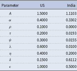
Following the calibration, the optimized parameter values were validated by comparing the simulated outputs with the actual data for both the United States and India, ensuring the robustness of the estimation. The final calibrated values for each parameter are presented in Table 2. The inclusion of India in the calibration process is motivated by several key factors. First, India represents one of the largest and fastest-growing economies in the world, with significant industrialization and urbanization trends that contribute to both economic expansion and environmental challenges. Given the scope of our model, which examines the interplay between economic growth, pollution, and government intervention, India provides a particularly relevant case study due to its rapid economic development and increasing environmental concerns.
Optimized parameter values for the US and India

Second, India’s fiscal policies, including government spending and taxation strategies, exhibit substantial differences from those of more developed economies such as the United States. These distinctions allow for a broader evaluation of how varying levels of government intervention impact long-term economic and environmental sustainability. The calibration results highlight these contrasts, with India displaying different parameter values for public spending, taxation, and pollution sensitivity.
Furthermore, India’s policy decisions regarding environmental regulations, public debt, and capital investment offer valuable insights into the global challenges of balancing economic development with sustainability. By incorporating India into our analysis, we aim to capture a more comprehensive picture of economic-environmental dynamics across diverse economic structures, strengthening the generalizability and applicability of our findings.
It is interesting to note that the damage caused by pollution, parameterized by
 $\rho$
, appears lower for India (rounded to zero in the table due to numerical precision), likely because the magnitude of India’s data is smaller. Additionally, the calibration suggests that the US have higher spending than taxation, while the opposite holds for India. After calibration, we simulated the future trajectories of the variables for India and the US using both the calibrated parameters and scenarios where
 $\tau$
and
 $\psi$
were increased or decreased by 20%. A crucial insight from these simulations is that, if no changes are made compared to the last 25 years (i.e., using the calibrated parameters), future projections indicate that extremely high-pollution levels will damage capital, ultimately driving it to zero in the long run. Consequently, pollution levels will also decrease, but this cannot be considered a positive outcome since lower pollution results from a collapsing economy. This effect is particularly pronounced in countries like India, where economic decline is severe, while in the US, the downturn occurs more gradually through boom-and-bust cycles that eventually stabilize at extremely low levels of capital (as shown in Figure 3).
Simulations of K and P over 50 periods using the calibrated parameters.

As previously discussed, further simulations were conducted to assess the impact of modifying
 $ \tau$
and
 $ \psi$
.
As seen in Figure 4, altering these parameters does not significantly affect capital accumulation in the US. The only observed change is that an increase in
 $ \tau$
shifts the timing of capital oscillations without reducing their amplitude. A similar effect is observed for pollution, as depicted in Figure 5.
Simulations of K over 50 periods, modifying the values of
 $\tau$
and
 $\psi$
. The red line represents the series with calibrated parameters, while the blue line represents the modified series. When only one line is visible, it indicates that the two simulations overlap.

Simulations of P over 50 periods, modifying the values of
 $\tau$
and
 $\psi$
. The red line represents the series with calibrated parameters, while the blue line represents the modified series. When only one line is visible, it indicates that the two simulations overlap.

For India, the same pattern holds: even increasing
 $ \tau$
does not induce substantial changes, reinforcing the idea that these parameters alone do not drive long-term economic and environmental outcomes in the model. Overall, the calibration results highlight the strong negative feedback loop between excessive pollution and economic decline, particularly for economies with already lower capital levels such as India. The findings indicate that, in the absence of corrective policies, pollution-induced capital destruction could become self-reinforcing, leading to economic stagnation. Moreover, the inability of modest changes in
 $ \tau$
and
 $ \psi$
to alter long-term trajectories suggests that deeper structural reforms or stronger policy interventions may be necessary to prevent catastrophic economic downturns. These insights emphasize the importance of proactive environmental and economic strategies to sustain long-term economic viability.
5. Conclusion
The analysis of global dynamics highlights several significant findings regarding the interplay between government intervention, initial economic conditions, and individual decisions related to environmental protection. One of the key insights from this study is the phenomenon of multistability—different economies can reach multiple possible equilibria depending on their initial starting points and the type of government intervention in place. The presence of multiple fixed points underscores the importance of considering both initial conditions and policy choices when addressing long-term economic and environmental sustainability. We observe that a combination of external factors, such as production damage and individual preferences for environmental utility, shapes capital accumulation, pollution levels, and government budget outcomes. The interaction between these parameters and the level of government intervention produces varying outcomes in equilibrium, with significant trade-offs between economic growth and environmental quality.
When starting from low levels of capital and pollution, the system tends to stabilize with higher capital and moderate pollution levels. However, starting with higher levels of capital and pollution often leads to a lower capital equilibrium with higher pollution. This pattern is particularly pronounced under low or intermediate government intervention. The underlying reason for this divergence lies in individual decisions about environmental investment. In low or intermediate government intervention cases, much of the responsibility for environmental protection falls on individuals. Since people tend to invest in environmental preservation only when pollution levels are not too high, economies with initially low pollution experience positive feedback: individuals continue to invest in the environment, curbing pollution and allowing capital to grow. Conversely, economies starting with high-pollution levels face a negative feedback loop, where individuals reduce their environmental investments due to high pollution, leading to further environmental degradation and lower capital levels in equilibrium. In the case of high government intervention, the results shift. Here, we see that capital levels in equilibrium are higher, but this comes at the cost of increased pollution. High government intervention fosters capital accumulation by boosting economic activity, but without sufficient environmental policies, it also leads to more pollution. This highlights a critical trade-off: high government intervention promotes capital growth but often at the expense of environmental sustainability. Additionally, calibration results reveal a strong negative feedback loop between pollution and economic decline. Without corrective policies, pollution-driven capital loss could become self-reinforcing, leading to stagnation. Furthermore, minor adjustments in economic policies may fail to alter long-term trends, suggesting the need for deeper structural reforms or stronger policy interventions to avert economic collapse.
Competing interests
No relevant or material financial interests related to the research described in this paper.
Funding
Thomas Seegmuller acknowledges financial support from the French government under the “France 2030”investment plan managed by the French National Research Agency Grant ANR-17-EURE-0020, and by the Excellence Initiative of Aix-Marseille University – A*MIDEX.
Appendix A. Proof of propositions
Appendix A.1 Proof of Proposition1
From Assumption1 we know that
 $n_{max}=\min (w_t,n^{(p)})$
and it is easy to verify that
-
• in case
$\lambda \ge \lambda _1$
or
$\lambda \lt \lambda _1 \wedge P\ge P^{(\lambda)}$
, it has
$n_{max}=w_t$
; -
• in all other cases,
$n_{max}=n^{(p)}$
.




where
 $P^{(\lambda)}$
is the value of
 $P$
that solves
 $\frac {(\lambda _1-\lambda)AK^\alpha }{1-\delta }=P+\rho P^3$
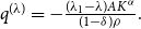
and thanks to Cartano method it is possible to give its analytical form:
 \begin{equation*} P^{(\lambda)} = \sqrt [3]{-\frac {q^{(\lambda)}}{2} + \sqrt {\left (\frac {q^{(\lambda)}}{2}\right)^2 + \left (\frac {p}{3}\right)^3}} + \sqrt [3]{-\frac {q^{(\lambda)}}{2} - \sqrt {\left (\frac {q^{(\lambda)}}{2}\right)^2 + \left (\frac {p}{3}\right)^3}} \end{equation*}
with
 $p=1/\rho$
and
 $q^{(\lambda)}=-\frac {(\lambda _1-\lambda)AK^\alpha }{(1-\delta)\rho }.$
Consider now the objective function given by (10):
 \begin{equation*} OBJ=\ln \left (r_{t+1} (w_t - n_t) \right) - \epsilon \ln \left [(1-\delta)P_t + \lambda Y_t - \eta n_t\right ] \end{equation*}
and its derivative
 \begin{equation*} \frac {\partial OBJ}{\partial n_t}=\frac {\epsilon \eta }{(1-\delta)P_t+\lambda Y_t-\eta n_t}-\frac {1}{w_t-n_t} \,. \end{equation*}
Then
-
• In case
$\epsilon \gt 1$
function
$OBJ$
has a maximum in
$n^*$
and-
– if
$\lambda \ge \epsilon \lambda _1$
or
$\lambda \lt \epsilon \lambda _1 \wedge P_t\ge P^{(\epsilon)}$
it has
$n^*\lt 0$
therefore
$n_t=0$
is the solution for the optimization problem; -
– if
$\lambda \lt \lambda _1 \wedge P_t\lt P^{(\lambda)}$
it has
$n^*\gt n_{max}=n^{(p)}$
therefore
$n^{(p)}$
is the solution for the optimization problem; -
– in all other cases
$0\lt n^*\lt n_{max}$
therefore
$n^*$
is the solution for the optimization problem;
-
-
• In case
$\epsilon \lt 1$
function
$OBJ$
has a minimum in
$n^*$
and-
– if
$n_{max}=w$
it has
$n^*\gt w$
therefore
$OBJ$
is decreasing in
$n_t$
and
$n_t=0$
is the solution for the optimization problem; -
– otherwise
$n_{max}=n^{(p)}$
is the solution of the optimization problem;
-









Note that
 $P^{(\epsilon)}$
is the real solution of
 $P_t+\rho P_t^3=\frac {\epsilon \lambda _1-\lambda }{1-\delta }AK_t^\alpha$
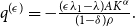
and thanks to Cartano method it is possible to give its analytical form:
 \begin{equation*} P^{(\epsilon)} = \sqrt [3]{-\frac {q^{(\epsilon)}}{2} + \sqrt {\left (\frac {q^{(\epsilon)}}{2}\right)^2 + \left (\frac {p}{3}\right)^3}} + \sqrt [3]{-\frac {q^{(\epsilon)}}{2} - \sqrt {\left (\frac {q^{(\epsilon)}}{2}\right)^2 + \left (\frac {p}{3}\right)^3}} \end{equation*}
with
 $p=1/\rho$
and
 $q^{(\epsilon)}=-\frac {(\epsilon \lambda _1-\lambda)AK^\alpha }{(1-\delta)\rho }.$
Appendix A.2 Proof of Proposition2
The equilibrium points of the dynamic system are defined as those for which the key variables remain constant over time, i.e.
 $P_{t+1}=P_t$
,
 $B_{t+1}=B_t$
,
 $K_{t+1}=K_t$
.
We consider the case with
 $n_t=n^*$
, therefore
 $\epsilon \gt 1$
,
 $\lambda \lt \epsilon \lambda _1$
and
 $P_t\lt P^{(\epsilon)}$
. The fist equation of system
 $T$
given in (12) models the evolution of capital. Note that, considering that in case
 $n_t=n^*$
the FOC (11) becomes
 \begin{equation*} \frac {r_{t+1}}{c_{t+1}}=\frac {\epsilon \eta }{P_{t+1}} \end{equation*}
we can rewrite the equation of pollution levels as
 \begin{equation*} P_{t+1}=\epsilon \eta (w_t-n_t)=\epsilon \eta (K_{t+1}+B_{t+1}) \end{equation*}
and considering that
 $n_t=w_t-K_{t+1}-B_{t+1}$
in the accumulation of pollution, we get:
 \begin{equation*} \eta (\epsilon -1)(K_{t+1}+B_{t+1})=(1-\delta)\epsilon \eta (K_t+B_t)+[\lambda -\eta (1-\alpha) (1-\tau)]Y_t \end{equation*}
with
 $Y_t=AK^\alpha /(1+\rho P^2)$
. It follows that we can write
 \begin{equation*} K+B=\frac {(\lambda -\lambda _1)AK^\alpha }{(1+\rho P^2)(\epsilon \delta -1)\eta } \end{equation*}
and the equilibrium points are values of
 $K$
that satisfy
 \begin{equation} K=\mathcal{K}(K)\, \end{equation}
with
 \begin{equation*} \mathcal{K}(K)=\frac {(\lambda -\lambda _1)AK^\alpha }{(1+\rho P^2)(\epsilon \delta -1)\eta }-B. \end{equation*}
The lhs of Eq. (A.1) is the identity line, while function
 $\mathcal{K}(K)$
is strictly increasing (decreasing) and concave (convex) for
 $\epsilon \delta \gt 1\wedge \lambda \gt \lambda _1$
or
 $\epsilon \delta \lt 1\wedge \lambda \lt \lambda _1$
(otherwise). Moreover it has
 $\mathcal{K}(0)=-B$
,
 $\lim _{K\to 0}\mathcal{K}^\prime =\infty$
,
 $\lim _{K\to \infty }\mathcal{K}^\prime =0$
. It follows that
-
• in case
$\epsilon \delta \gt 1\wedge \lambda \gt \lambda _1$
or
$\epsilon \delta \lt 1\wedge \lambda \lt \lambda _1$
-
• in case
$\epsilon \delta \gt 1\wedge \lambda \le \lambda _1$
or
$\epsilon \lambda \lt 1\wedge \lambda \ge \lambda _1$
eq. (A.1) has no solutions.






The second equation of system
 $T$
is linear in
 $B$
and it always has a fixed point equilibrium given by
 \begin{equation*} B^*=\frac {(\psi -\tau)AK^\alpha }{1+\rho P^2-(1-\tau)\alpha AK^{\alpha -1}}. \end{equation*}
Note that
 $B^*$
is negative if
 $r\gt 1 \wedge \psi \lt \tau$
or
 $r\lt 1 \wedge \psi \gt \tau$
.
The solution of the last equation of system
 $T$
is given by the value
 $P$
that solve
 \begin{equation*} P+\rho P^3=\frac {\epsilon (\lambda _1-\lambda)AK^\alpha }{1-\epsilon \delta }. \end{equation*}
Previous equation has no solution for
 $\epsilon \lt 1/\delta \wedge \lambda \gt \lambda _1$
or
 $\epsilon \gt 1/\delta \wedge \lambda \lt \lambda _1$
otherwise it has a unique real solution given by
 \begin{equation*} P^{*}=\sqrt [3]{-q + \sqrt {q^2 + \frac {1}{27\rho ^3}}} + \sqrt [3]{-q - \sqrt {q^2 +\frac {1}{27\rho ^3}}} \end{equation*}
where
 \begin{equation*} q=-\frac {\epsilon (\lambda _1-\lambda)AK_t^\alpha }{2(1-\epsilon \delta)\rho }. \end{equation*}
Under the conditions for which
 $n^*$
is the solution of the optimization problem, the point
 $P^*$
satisfies
 $P^*\lt P^{(\epsilon)}$
,
 $P^*\gt P^{(\lambda)}$
.
We can conclude that
-
• In case
$\epsilon \delta \gt 1\wedge \lambda \gt \lambda _1$
or
$\epsilon \delta \lt 1\wedge \lambda \lt \lambda _1$
-
–
$r\gt 1 \wedge \psi \lt \tau$
or
$r\lt 1 \wedge \psi \gt \tau$
a unique fixed point equilibrium exists given by
$E^*\equiv (K^*, B^*, P^*)$
-
–
$r\gt 1 \wedge \psi \gt \tau$
or
$r\lt 1 \wedge \psi \lt \tau$
at most two fixed points exist given by
$E^{*1}\equiv (K^{*1}, B^{*1}, P^{*1})$
and
$E^{*2}\equiv (K^{*2}, B^{*2}, P^{*2})$
-
-
• otherwise no fixed point exists









with
 $K^{*1}\lt K^{*2}$
and
 \begin{equation*} B^{\circ }=\frac {(\psi -\tau)A{(K^{\circ }})^\alpha }{1+\rho {(P^{\circ })}^2-(1-\tau)\alpha A{(K^{\circ })}^{\alpha -1}}, \end{equation*}
 \begin{equation*} P^{\circ }=\sqrt [3]{-q^\circ + \sqrt {(q^\circ)^2 + \frac {1}{27\rho ^3}}} + \sqrt [3]{-q^\circ - \sqrt {(q^\circ)^2 +\frac {1}{27\rho ^3}}}, \end{equation*}
 \begin{equation*} q^\circ =-\frac {\epsilon (\lambda _1-\lambda)A(K^\circ)^\alpha }{2(1-\epsilon \delta)\rho }, \quad \circ \in \{*, *1, *2\}. \end{equation*}
Appendix A.3 Proof of Proposition3
Here we consider the fixed points arising for
 $n_t=0$
. Considering that in the fixed points it has
 $K_{t+1}=K_t=K$
,
 $B_{t+1}=B_t=B$
and
 $P_{t+1}=P_t=P$
, the first equation of system
 $T$
can be written as
 \begin{equation*} \frac {(1-\tau)(1-\alpha)A}{1+\rho P^2}K^\alpha -K=B. \end{equation*}
The lhs of previous equation is equal to zero for
 $K=0$
it tends to
 $-\infty$
as
 $K\to \infty$
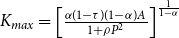
and it is unimodal with maximum in
 $K_{max}=\left [\frac {\alpha (1-\tau)(1-\alpha)A}{1+\rho P^2}\right ]^{\frac {1}{1-\alpha }}$
. Therefore
-
• for
$B\le 0$
previous equation always has one solution
$K^\dagger$
-
• for
$B\gt 0$
previous equation may have up to two solutions
$K^{\dagger 1}\lt K^{\dagger 2}$
.


As the second equation is concerned, the same results of proof 2 holds.
Lastly, fixed points of
 $P$
are solution of
 \begin{equation*} P(1+\rho P^2)=\frac {\lambda A K^\alpha }{\delta } \end{equation*}
and, considering the range of parameters values for which the condition
 $n_t=0$
holds, it follows that previous equation has one solution if one of the following is satisfied:
-
•
$\epsilon \gt 1 \wedge \lambda \ge \delta \epsilon \lambda _1$
-
•
$\epsilon \lt 1 \wedge \lambda \ge \delta \lambda _1$


We can conclude that
-
• In case
$\epsilon \gt 1 \wedge \lambda \ge \delta \epsilon \lambda _1$
or
$\epsilon \lt 1 \wedge \lambda \ge \delta \lambda _1$
-
–
$r\gt 1 \wedge \psi \lt \tau$
or
$r\lt 1 \wedge \psi \gt \tau$
a unique fixed point exists given by
$E^\dagger \equiv (K^\dagger, B^\dagger, P^\dagger)$
-
–
$r\gt 1 \wedge \psi \gt \tau$
or
$r\lt 1 \wedge \psi \lt \tau$
up to two fixed points may exist given by
$E^{\dagger 1}\equiv (K^{\dagger 1}, B^{\dagger 1}, P^{\dagger 1})$
and
$E^{\dagger 2}\equiv (K^{\dagger 2}, B^{\dagger 2}, P^{*2})$
-
-
• otherwise no fixed point exists






with
 $K^{\dagger 1}\lt K^{\dagger 2}$
and
 \begin{equation*} B^{\circ }=\frac {(\psi -\tau)A{(K^{\circ }})^\alpha }{1+\rho {(P^{\circ })}^2-(1-\tau)\alpha A{(K^{\circ })}^{\alpha -1}}, \end{equation*}
 \begin{equation*} P^{\circ }=\sqrt [3]{-q^\circ + \sqrt {(q^\circ)^2 + \frac {1}{27\rho ^3}}} + \sqrt [3]{-q^\circ - \sqrt {(q^\circ)^2 +\frac {1}{27\rho ^3}}}, \end{equation*}
 \begin{equation*} q^\circ =-\frac {\lambda A(K^\circ)^\alpha }{2\delta \rho }, \quad \circ \in \{\dagger, \dagger 1, \dagger 2\}. \end{equation*}
Appendix B. Global dynamics—simulations result
In this appendix, we provide a comprehensive analysis of the equilibrium values for the key variables
 $K$
(capital),
 $P$
(pollution), and
 $B$
(government budget) across different economic scenarios. We evaluate the impact of government intervention at three levels: low, medium, and high. We further analyze how the equilibrium values change according to the initial conditions and the parameters
 $\lambda$
and
 $\epsilon$
, representing the pollution damage and individuals’ environmental utility, respectively. These analyses are presented in graphical form and summarized in tables for each scenario. The detailed results allow us to observe not only the existence of equilibrium points but also the specific values of the variables at those points, providing insights into the system’s long-term behavior.
Appendix B.1 Simulation results
See Appendix Tables B1, B2 and B3.
Values of K in equilibrium. Gov: government intervention. I.C.: initial conditions

Values of B in equilibrium. Gov: government intervention. I.C.: initial conditions

Values of P in equilibrium. Gov: government intervention. I.C.: initial conditions

Values of K in equilibrium depending on parameters value.

Values of B in equilibrium depending on parameters value.

Values of P in equilibrium depending on parameters value.