1. Introduction

Malcolm Forster and Elliott Sober (Reference Forster and Sober1994) have appealed to a concept of predicted fit to defend the Akaike Information Criterion as a criterion for model selection in scientific inference. Given assumptions about errors in the data, fit of a model to the data is not always a good indication of how well the model will fit future data, as a model that fits the data too closely is likely to be tracking random errors in the data in addition to the lawlike phenomenon under investigation. An important contribution of their work has been its challenge to the assumption that fit to data exhausts the empirical criteria for scientific inference. This unwarranted assumption of naïve empiricism has contributed to unjustified scepticism about the objectivity of scientific inference.

Akaikean and other statistical methods can be useful tools of scientific inference. They cannot, however, be the whole of scientific inference, for two reasons: such methods do not function in a self-sufficient manner and must be supplemented by other considerations in order for them to be useful, and statistical methods by themselves do not satisfy all the goals of scientific inference, one of which is anticipation of the results of novel experiments. We argue that accurate measurement of causal parameters by phenomena is an important goal of scientific inference, both in its own right and for its contribution to prediction and its extension to novel experiments. These considerations undermine Sober's appeal (this volume) to Akaikean methodology to support an instrumentalist account of scientific inference.

2. Model Selection

A few remarks about terminology are in order We want to consider situations in which data is generated via some process, such as an experiment or a series of observations. Such a process may include errors or other elements that are to be regarded as stochastic (whether or not there is some underlying deterministic law). Following Linhart and Zucchini (Reference Linhart and Zucchini1986), we will use the word “model” for a probability distribution over possible data sets. A model is therefore fully specified and confers a definite probability on any data set. Our terminology differs, therefore, from that of Forster and Sober, who use the word “model” for what, in our terminology, is a family of models; if this difference is borne in mind, then no confusion should result. We will therefore assume that there is some probability distribution f *(X) that specifies the probability that a body of data X will be the one that is actually obtained. This distribution, which will be called the “true model,” will initially be unknown or incompletely known; it is the task of statistical inference to gain information about it from the data. Expectation values with respect to the true model will be denoted by E*[ · ]. Of particular interest are families of models f(X| θ) that depend on some vector of parameters θ.

Given a model f and a body of data X, the likelihood is defined as L = f(X); we will also write L(θ) = f(X| θ). The log-likelihood l(θ) is given by l(θ) = log(L(θ)). If there is a unique vector of parameters that maximizes the likelihood (and ipso facto the log-likelihood), this will be denoted by $\hat{\theta }$.

A statistical model is meant to be, in some sense, an approximation to the process by which the data is generated. The task of selecting a model based on a body of data involves several decisions. First, one must decide what is to count as a good fit of our model to the unknown or incompletely known process that generates the data. That is, one must decide on a discrepancy, a low value of which is to be regarded as a good match between our model and the truth. Second, one must choose families of models from which the model is to be selected. One then adopts a method designed to select from among these models one with a low discrepancy.

A naïve empiricism might regard closeness of fit of the model to the data as the goal of model selection. Forster and Sober (Reference Forster and Sober1994) have done a good job of arguing that this is unacceptable—and moreover, unacceptable on empirical grounds. Because of the phenomenon of overfitting, closeness of the model to the data is not always an indication of how close the model will fit future data, as a model that fits the data too closely is likely to be tracking random errors in the data in addition to the lawlike phenomenon under investigation. If one is interested in predictive success, then the criterion chosen should not be based solely on the fit of the model to the data.

The Akaike Information Criterion is designed to yield a model with a low value of the Kullback-Leibler discrepancy:

or, what is the same thing, to yield a model with high expected log-likelihood,

where the expectation value is taken with respect to a repetition of the same experiment—that is, the same process whereby the original data was generated. Forster and Sober refer to the expected log-likelihood as “predictive accuracy.” If log-likelihood is regarded as a measure of the accuracy of prediction, then there is some justification for this terminology. As Forster points out in his contribution to this symposium, the expected log-likelihood must be taken with respect to a repetition of the same experiment. A high value of l*(θ) does not guarantee that the model will work well if the data-gathering process is changed to include a wider range of data. To use Forster's terminology: it is the goal of the Akaike procedure to maximize interpolative accuracy, not extrapolative accuracy. A high value of interpolative accuracy does not guarantee that the model will continue to do well under novel circumstances.

As a simple example, consider the following. Let our data consist of 100 independently identically distributed pairs of numbers (x _i, y _i), where the x _i's are chosen according to a uniform distribution on the interval [−1, 1], and the y _i's are normally distributed, with variance 1, about g*(x _i), where g* is the gaussian function

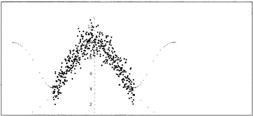
Take as the kth family of models linear combinations of the first k elements of the series of functions {1, sin(π x), cos(π x), sin(2π x), cos(2π x), . . .}. It turns out that k = 5 tends to give a good fit, whereas for higher values of k overfitting sets in. Figure 1 shows a typical data set, together with the best-fit curve using 5 basis functions to that data and the extrapolation of that best-fit curve beyond the interval [−1,1]. It should be emphasized that we are not here engaged in mere grue-mongering, but rather wish to make the point that a method designed to reward interpolative predictive accuracy—that is, expected fit upon repetition of the same data-generating process—won't tend to be sensitive to matters that are irrelevant to interpolative predictive accuracy.

Figure 1.

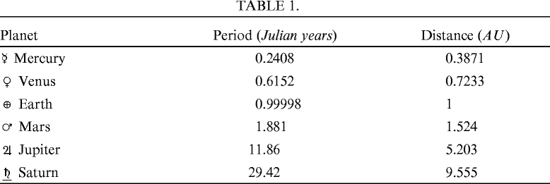
The term “interpolative predictive accuracy” is potentially misleading. What the Akaikean methodology strives to maximize is expected log-likelihood upon a repetition of the same experiment. Success at this task—the task for which the method was designed—need not extrapolate to novel situations, whether the new data points are found between or beyond the original data points. To illustrate this, consider the task of finding a relation between planetary distances and periods. The actual values are given in Table 1.

Table 1

Planet	Period (Julian years)	Distance (AU)
☿ Mercury	0.2408	0.3871
♀ Venus	0.6152	0.7233
⊕ Earth	0.99998	1
♂ Mars	1.881	1.524
♃ Jupiter	11.86	5.203
♄ Saturn	29.42	9.555

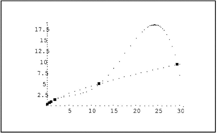
Figure 2 shows Kepler's harmonic law T ∝ R ^3/2, and a quartic law T = a + bR + cR ² + dR ³ + eR ⁴ that closely fits the data. Suppose that any further data we expect to gather will consists of more measurements of the positions and periods of the planets. In this case, the quartic curve has higher predictive accuracy, because it comes closer to the actual values. Clearly though, it will be less reliable when it comes to predicting results at intermediate distances.

Figure 2.

The Akaike procedure is applicable to cases in which we have several families F _k of models to choose from.Footnote ¹ Let the family F _k be parameterized by the vector θ _k. The Akaike methodology begins by selecting from each family k the maximum likelihood model ƒ _k(X| $\hat{\theta }_{k}$) One is now faced with a choice of which of these maximum likelihood models to select.

Associated with each family F _k is the quantity

that measures the average performance of this family under the procedure of generating data and then picking the maximum-likelihood vector of parameters. If we knew l*(k) for each family, then it would behoove us to use a family that has a high value for this quantity, on the grounds that this yields a high expectation value for the predictive accuracy of the maximum-likelihood model.Footnote ² The epistemic situation in which one confronts a typical model-selection problem is typically one in which we don't know l*(k). This is where Akaike's theorem comes in. This theorem states that, under certain regularity conditions,

where dim(F _k) is the dimension of the parameter space of the family F _k. That is: the quantities l( $\hat{\theta }_{k}$) − dim(F _k) and l*( $\hat{\theta }_{k}$) vary around the same mean, or, in other words, l( $\hat{\theta }_{k}$) − dim(F _k) is an unbiased estimator of l*( $\hat{\theta }_{k}$). For the curve-fitting case, in which linear combinations of a certain set of functions are to be fit to the data, then this relation holds if the errors are normally distributed about their true values. In general it applies to any case in which the maximum-likelihood parameters are normally distributed about the optimal values of the parameters—a condition that is approached asymptotically for a wide variety of model selection tasks.

The quantity l($\hat{\theta }_{k}$) − dim(F _k) is calculable from the data and, in the cases to which Akaike's theorem applies, is an unbiased estimator of l*($\hat{\theta }_{k}$). Akaikean methodology recommends that we choose the maximum-likelihood model from the family for which l*($\hat{\theta }_{k}$) − dim(F _k) has the largest value among all the families considered, or, equivalently, that we choose the family for which

has the least value.

One reason that this methodology cannot be all there is to scientific inference should be fairly clear: the method leaves it open what families of models to use. Success can depend on a judicious choice of families. Suppose, then, we have made a judicious choice of families of models to fit to the data, aided by background knowledge, and have applied the Akaike procedure. What are we entitled to infer about the selected model?

One is tempted to conclude that the predictive accuracy of the selected model, l*($\hat{\theta }$), is probably close to l($\hat{\theta }$) − dim(F _k). This temptation is encouraged by the terminology that refers to one as an “estimator” of the other. One might even suppose that the Akaike method presupposes the cogency of this conclusion. After all, l*( $\hat{\theta }$) is the quantity we wish to maximize, and we attempt to do it by choosing the largest value of l*( $\hat{\theta }$) − dim(F _k). Such a conclusion, however, requires an additional premise, namely, that these quantities have relatively small dispersions about their means. Only if this condition is satisfied do we have a right to conclude that the two quantities are probably close.

This is not a condition that is satisfied in all situations to which the AIC is applied. It can happen—and this may even be the typical case—that the variance of AIC(k) is large compared to the differences in the mean values of AIC(k) for different values of k. That this does not invalidate the Akaike method stems from the decision-theoretic rationale of the method. If methods are to be judged by their expected performance, then the Akaike method need not provide a reliable answer to the question of how close the selected model is to the truth (a question that, without further ado, it does not answer), if it can be shown to have better expected performance than other proposed methods.

The success of the Akaikean methodology, when it succeeds, is cashed out in terms of the expected value of the interpolative predictive accuracy of the selected model, which may or may not carry over to new situations.

3. Measuring Causal Parameters

Is this all that we can expect to gain from empirical data? That it is not can be illustrated by returning to Kepler's laws and considering the use to which Newton put them. Newton was able to show (Principia Bk. 1, Prop. 1 and 2) that Kepler's area law is equivalent to the proposition that the acceleration of each planet is directed toward the sun. Moreover, any deviation from the area law would carry information about the direction of the planet's acceleration Β a change in the rate at which the radius vector from the sun sweeps out area indicates a component of acceleration perpendicular to the radius vector. An increase in the areal rate indicates that the net acceleration of the planet is not directed at the sun but somewhat ahead of it; a decrease in the areal rate indicates an acceleration that deviates from the central in the opposite direction.

The accelerations of the planets, therefore, are directed toward the sun, or very nearly so. By Newton's second law, this entails that the force on each planet is directed toward the sun, or very nearly so. This suggests that we look for a law-like dependence of the magnitude of acceleration on distance from the sun.

Newton showed that, if the planetary orbits are ellipses with the sun at a focus, the acceleration of the planet toward the sun at the moment that its distance from the sun is equal to the semi-major axis of the ellipse is given by

where T is the period of the planet's orbit and R is the semi-major axis of its orbit.Footnote ³ The dependence of the periods of the planets on their distances from the sun, therefore, carries information about the dependence of the planetary accelerations on distance from the sun. If one suspects that such dependence will be given by a power law, then this is motivation for seriously considering a power law for the dependence of period on distance. Given the above relation between elliptical and concentric circular orbits, Newton's Corollary 7 of Proposition 4, Book I,

can be applied to infer the inverse-square power law for centripetal acceleration from the harmonic law for the planetary orbits (see Harper Reference Harper1999). Kepler's harmonic law, according to which T ∝ R ^3/2, therefore, dictates that the acceleration of the planets toward the sun be an inverse square law. Moreover, if the harmonic law is only approximately correct, then the dependence of acceleration on distance is approximately an inverse square law.

An independent measure of the dependence of acceleration on distance from the sun is given by the absence of precession. Newton showed (Principia Bk. 1, Cor. 1 Prop 45) that the orbit of a body is an ellipse with acceleration toward a focus, precessing at a rate of p degrees per revolution, if and only if the centripetal force acting on the body is given by the power law

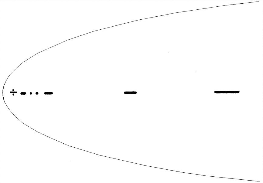
At a lecture given by Harper on Newton's argument, Howard Stein asked how the evidence Harper had cited from Newton for the inverse-square law for gravitation toward the sun—the absence of significant orbital precession for each orbit and Kepler's harmonic law for the system of those six orbits—gave evidence against a hypothesis for variation of force with distance that agreed with the inverse-square in the distances explored by each orbit and in the inverse square relation among the forces at those six small distance ranges, but differed wildly from the inverse-square power law in the large ranges of distance not explored by the motions of those planets.

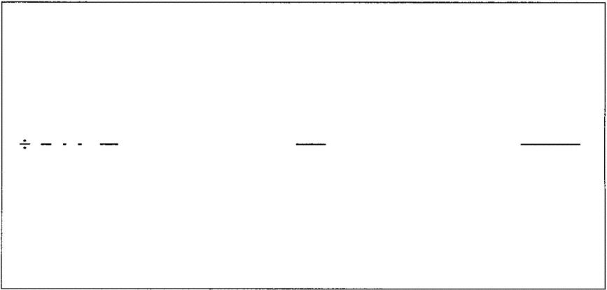
Figure 3 shows the approximate ranges of distances explored by each planet computed from the mean distances and eccentricities assigned to their orbits today.Footnote ⁴ A hypothesis corresponding to Stein's challenge might be given, for example, by one of the bizarre curves discussed above that result from using polynomials to fit to the data Kepler used to find the harmonic law. As we have seen above, and as Forster points out in his paper, the proof of Akaike's theorem shows that the Akaike criterion of predicted fit applies to future repetitions of the same experiment, but does not apply to extensions (or interpolations)Footnote ⁵ to ranges of independent variables not covered in the data set. For any given body of data about the periods and mean distances of the planetary orbits, however large, we can construct an alternative hypothesis that will mimic the harmonic law in the distances explored by the six planets but will do arbitrarily complex things in the distances not so explored. The Akaike criterion is not designed to meet challenges such as Stein's and it cannot be applied to do so, because it is helpless to reject such hypotheses.

Figure 3.

The distances explored by the planetary orbits.

Stein has argued that Newton's discussion of centripetal force and its three measures—motive, accelerative, and absolute—make it clear that what Newton counts as centripetal forces are what we would call acceleration fields (see Stein Reference Stein and Stuewer1970, 265–266 and Reference Stein1991, 211–213). The motive measure of a centripetal force on a body is its mass times its centripetal acceleration. The accelerative measure is the acceleration produced and is referred to distances from the center. That there should be an accelerative measure—that at each place around the center there is a quantity that is measured by the equal accelerations that would be produced on unsupported bodies at that distance—is what makes a centripetal force count as an acceleration field. The absolute measure of such a centripetal acceleration field is its strength. The harmonic law ratio for a system of orbits about a common center requires that the orbits exhibit centripetal accelerations corresponding to a single inverse square centripetal acceleration field. The ratio of the absolute measures of two such centripetal acceleration fields is the common ratio of the accelerations they would produce at any equal distances from their respective centers.

The following comments indicate the important role Stein sees for the concept of an acceleration field in Newton's argument for the inverse-square law.

This comment was preceded by the following comment about the extent to which Newton's induction is convincing.

The kinematical relation was the centripetal direction and inverse-square relation of the accelerations of these six planets. What Newton was lucky enough to find was the dynamical significance of Kepler's orbital laws. It is this dynamical significance that transforms the exponent in Kepler's harmonic law into a measure of a causally relevant parameter, namely, the exponent in the power law for a centripetal acceleration field directed toward the sun.

For any given distance from the center of the sun, the inverse-square adjusted centripetal accelerations exhibited by the planets count as agreeing measurements of the acceleration toward the sun that the sun-centered inverse-square acceleration field would produce on bodies at that distance. The estimate of the centripetal acceleration at distance d yielded by a given planetary orbit is given by

where R is the semi-major axis of the orbit and T is its period. For example, consider d = 7 A.U. The estimates of the acceleration at this distance yielded by the data (see Table 1) for each of the six planets is given in Table 2. It is the conviction that one is estimating this causally relevant parameter that warrants the extrapolation to distances other than those explored by the data. By way of contrast, the coefficients appearing in our polynomial fit are merely curve-fitting parameters, without the sort of dynamical significance that would lead one to expect that the fitted polynomials should continue to give the right results in regions beyond the data.

Table 2

Planet	Mercury	Venus	Earth	Mars	Jupiter	Saturn
Measure of Centripetal Acceleration at 7 AU	0.8060	0.8055	0.8057	0.8060	0.8069	0.8120

The alternative hypotheses suggested by Stein's challenge give up Newton's agreeing measurements of parameters of an inverse-square acceleration field without providing either a correspondingly rich realization of agreeing accurate measurements of proposed rival causal parameters or providing phenomena that would conflict with motion in accord with Newton's measurements.

Comets explore considerably more distances from the sun than the six small ranges explored by the primary planets known to Newton. In 1759 a particularly striking later vindication of extending the inverse-square law for an acceleration field toward the sun to distances not explored by planetary orbits was provided by Clairaut's celebrated success in predicting the return of Halley's comet. As early as 1705, Halley had proposed elements for this retrograde orbit with a perihelion distance of about .58 AU and a period of on average about 75.5 years, corresponding to a semi-major axis of about 17.86 AU and an eccentricity of about .97.Footnote ⁶

We want to claim that, in contrast to what would have been the case if legitimate scientific inference were limited to what could be justified by the Akaike criterion for predicted fit alone, it did not take empirical evidence sufficient for phenomena such as this comet orbit to be able to dismiss alternative hypotheses corresponding to Stein's challenge.

Newton offers additional measurements to back up his assumption that the inverse-square centripetal forces directed toward the sun, Jupiter, Saturn, and earth are acceleration fields.Footnote ⁷ These include pendulum experiments and the equality of the acceleration of terrestrial gravity at the surface of the earth with the inverse-square adjusted centripetal acceleration of the lunar orbit exhibited in the moon test. These put bounds on a parameter Δ _e representing differences in ratios of inertial mass to inverse-square adjusted weight towards the earth for bodies.Footnote ⁸ Newton's harmonic law data for Jupiter's moons and for Saturn's moons put bounds on the corresponding parameters Δ _j, and Δ _s for Jupiter and Saturn, while his harmonic law data for the orbits of the planets about the sun put bounds on Δ _h representing differences between ratios of inertial mass to inverse-square adjusted weight of bodies toward the sun. Additional bounds on Δ _h are provided by the absence of polarization with respect to the sun of the orbits of Jupiter's satellites, Saturn's satellites, and the orbit of the moon about the earth.Footnote ⁹ The measurements directly bounding Δ _h are backed up by the phenomena measuring bounds on Δ _e, Δ _j and Δ _s. All these phenomena count as agreeing measurements bounding toward zero a general parameter Δ representing differences between ratios of inertial mass to inverse-square adjusted weight toward solar system bodies.

Figure 4.

Halley's comet sweeps out a greater range of distances than those explored by planetary orbits.

In General Relativity these phenomena cited by Newton, together with far more precise phenomena made available from more recent Eötvös experiments and lunar laser ranging, count as agreeing measurements bounding toward zero an even more general parameter representing differences between inertial and passive gravitational mass.Footnote ¹⁰ These efforts at testing the Equivalence Principle as well as other research programs for developing testing frameworks for General Relativity very much conform to the goal of measuring causal parameters that guides Newton's inferences to inverse-square acceleration fields.Footnote ¹¹

In the later part of the nineteenth century Simon Newcomb based his improved model for calculating orbital ephemerides for predicting motions of the sun, moon, and planets on the development of a single consistent assignment of masses to the interacting solar system bodies.Footnote ¹² Newcomb's efforts were directed not just to accurate prediction of more precise phenomena but, rather, to accurate prediction in accordance with accurate estimates of these masses—causal parameters measured by the predicted phenomena. Today's orbital ephemerides are calculated according to a gravitational model that takes into account point mass interactions among the sun, moon, and planets together with corrections from General Relativity, as well as additional interactions such as the earth tide action on the moon.Footnote ¹³ The least squares adjustment of the model to such data as transit observations, radar ranging to planets, and lunar laser ranging is an adjustment that results in an assignment of values to the causal parameters of the model that count as better measured by these data.Footnote ¹⁴ Both the construction of Newtonian ephemerides by Simon Newcomb and the construction of ephemerides today, in accordance with General Relativity, are guided by the goal of prediction backed up by accurate measurement of causal parameters.