I. Introduction
The existing research on wine price prediction mainly deal with a cross-sectional analysis of wine prices, focusing on the prices at a particular point in time and their relationship to factors like weather, critical ratings, etc. Given that the primary focus of cross-sectional analysis is on explanation of the relationship between wine prices and a particular set of predictor variables, it is therefore unsurprising that parametric methods, particularly multiple linear regressions,Footnote 1 are most often used to predict wine prices (Ashenfelter, 2015; Storchmann, Reference Storchmann2012; Ashenfelter, Reference Ashenfelter2010; Jones and Storchmann, Reference Jones and Storchmann2001; Ashenfelter, 2001; Lima, Reference Lima2006). Thus, a hypothesized relationship between certain predictor variables (e.g. weather) and wine prices is made and linear regression is subsequently carried out to test the strength of that relationship.
This paper moves away from the cross-sectional analysis, which dominates the existing literature, and focuses purely on time series analysis, predicting wine returns based on a subset of previous return values. We treat the wine returns in our dataset as a stochastic process and employ machine learning techniques, specifically Gaussian processes, to model and predict the returns. The central question we seek to explore is the following: to what extent do complicated machine learning techniques like Gaussian process regression and multi-task feature learning outperform simpler time series regression models in predicting the prices of fine wine?
The importance of exploring this question is threefold: firstly, machine learning techniques (in fact, anything other than linear regression), though commonly used in the forecasting literature of other financial instruments (Ribeiro and Lopes, Reference Ribeiro, Lopes, Lu, Zhang and Kwok2011; Taylor and Hinton, Reference Taylor and Hinton2009; Lázaro-Gredilla and Titsias, Reference Lázaro-Gredilla and Titsias2011; Ou and Wang, Reference Ou and Wang2011), are completely unprecedented when it comes to wine price forecasting. This research is thus novel and would be beneficial to the larger field of wine price prediction. Secondly, one of the problems with wine price prediction based on previous price points is the lack of sufficient price points across time, especially with rare wines. Machine learning techniques, however, have been shown to work well with sparse data, and the field of wine price prediction will benefit from such techniques. Finally, wine differs from the majority of other financial instruments in three main ways: (1) it does not have a yield, (2) the supply of wine from a given vintage year is always monotonically decreasing, and (3) with most wines, the global supply is unknown and often has to be estimated. Together, these differences are arguably sufficient to put wine into a separate class of financial instrument altogether, and thus it would be interesting to see how the machine learning algorithms commonly used in forecasting for most other financial instruments fare on wine.
We start by giving a brief review of the machine learning and wine-finance literature surrounding this topic to better situate our research. Next, we present a quick overview of the wine data and fit basic ARMA and GARCH models used in most of the financial time series literature to the wine returns in our dataset, explaining their shortfalls in the process. We then go on to fit Gaussian process regression models. Following that, we incorporate relationships between the wines into the Gaussian process regression framework using multi-task feature learning. We conclude in the last section.
II. Related Work
Gaussian processes have been widely used in the forecasting of financial instruments with results which are comparable to other machine learning techniques like Bayesian vector autoregression models (Petelin et al., Reference Petelin, Sindelar, Prikryl and Kocijan2011) and superior to the simpler, classic time series models (Lázaro-Gredilla and Titsias, Reference Lázaro-Gredilla and Titsias2011; Ou and Wang, Reference Ou and Wang2011) A key problem in using Gaussian processes to model and predict time series data is the choice of the kernel function for the Gaussian process regression. However, there are a few resources describing the various kernel functions and how to combine them together to suit a particular regression problem or to capture a certain trend (Shawe-Taylor and Cristianini, Reference Shawe-Taylor and Cristianini2004; Duvenaud, Reference Duvenaud2014). The kernels used in our Gaussian process regression are based heavily on the combinations proposed in Duvenaud (Reference Duvenaud2014).
Multi-task learning has been used most frequently in the area of collaborative filtering (Argyriou et al., Reference Argyriou, Evgeniou, Pontil, Schölkopf, Platt and Hofmann2006, 2008; Phuong and Phuong, Reference Phuong and Phuong2008) to build recommender systems. Nevertheless, there has been existing research which uses multi-task learning in slightly more uncommon situations like time series forecasting (Bakker and Heskes, Reference Bakker and Heskes2003). Recently, there is some research in combining both Gaussian process regression and multi-task learning (Bonilla et al., Reference Bonilla, Chai and Williams2008; Yu et al., Reference Yu, Tresp and Schwaighofer2005), particularly for sparse data problems (Wang and Khardon, Reference Wang and Khardon2012).
In the wine-finance literature, there are several studies which deal with methods of estimating wine returns based on previous return values (Fogarty, Reference Fogarty2006; Burton and Jacobsen, Reference Burton and Jacobsen2001; Jaeger, Reference Jaeger1981). One of the key issues we face in our research is that some of the wines are traded infrequently and hence lack sufficient price data which makes the estimation of returns difficult. While we propose sparse machine learning based solutions, Fogarty and Sadler (Reference Fogarty and Sadler2014) and Fogarty and Jones (Reference Fogarty and Jones2011) both give an overview of several alternative regression and non-regression based approaches used in estimating returns for wines with infrequent sales.
In addition, there are also several studies which look at the relationship between wine returns and characteristics like critical ratings as well as the correlation between wine returns and other financial assets (Masset and Henderson, Reference Masset and Henderson2010; Masset and Weisskopf, Reference Masset, Weisskopf, Giraud-Heraud and M. Pichery2013; Sanning et al., Reference Sanning, Shaffer and Sharratt2008). From these relationships, we get more information on various other factors which could perhaps influence wine returns. While we do not look at correlations between wine returns and factors like critical ratings or other financial assets in our study, we note that this is an area that is potentially useful for further research.
Finally, we note there is some work in using machine learning techniques with wine data, but only in predicting wine quality (Zajc, Reference Zajc2012) and for matching wines with food (Theunissen, Reference Theunissen2015). So far, we have not seen anything related to using machine learning techniques to forecast wine returns.
III. Exploratory Data Analysis
Our wine data is provided by the Wine-Searcher website (http://www.wine-searcher.com/) through their API. Because of the sheer size of the database, however, we will focus the preliminary data analysis on smaller subset of 100 wines, namely the 100 wines in the Liv-Ex 100 wines index (April 2014 composition), which represents the price movements of 100 of the most sought-after fine wines for which there is a strong secondary market. The Liv-Ex 100 wines come from 5 regions (Bordeaux, Burgundy, Rhone, Champagne and Bolgheri) and 14 vintage years. Throughout this paper, we will only refer to the wines by their ID number and not their names since we feel that the length and similarity of some of the wine names would serve as nothing but an unnecessary distraction to the overall goal of this paper.
Data cleaning consists of first converting wine prices of these 100 wines into GBP and then standardizing the frequency of the wine prices. We chose to work with percentage returns
 $\bigg(\displaystyle{{\matrix{ {returns_t} \cr}} \over {\matrix{ {returns_{t - 1}} \cr}}} \; \; - {\rm } 1\bigg)$
instead of wine prices due to the fact that returns are generally more stationary. For each wine, we denote the observed percentage returns at the most recent time point as Y
T
, with the percentage returns at the previous time points as Y
T-1
, YT-2
and so on. We also assume that the returns are generated by a stochastic process defined as Y
t
+ εt, εt
being the value of a purely zero-mean random process at time t which is independent of Y
T
so that
 ${\rm {\open E}}$
(Yt
+ ε
t) = Yt
, for t = 1…T.
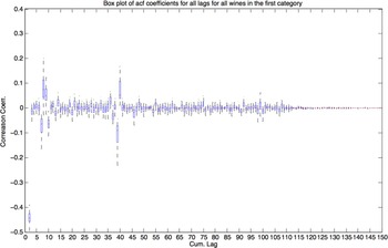
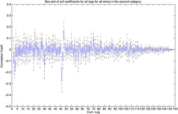
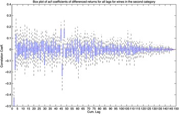
For almost all of the wines, the percentage returns at each time point tend to be constantly close to the mean of the series across time, with occasional spikes and dips which deviate significantly from the mean. There is slight evidence of volatility clustering, but no discernible upward or downward trend in the percentage returns of the wines. Looking at the sample autocorrelation function (acf) of percentage returns, that is, corr(YT,Yt−k ), for all the wines against lags (k) for all the lags up to the end of the each time series, we observe that half the wines show strong negative lag 1 temporal relationship, while the other half show a strong negative lag 1 temporal relationship in the first difference of the percentage returns.
A strong negative lag 1 temporal relationship is not uncommon in the returns of financial instruments. A likely explanation of this phenomenon in this case is a regression of wine prices to the mean, that is, large positive percentage returns tend to be followed by negative percentage returns and vice versa. It is slightly more difficult to venture an explanation for the autocorrelation structure observed in the second category since it appears to be more complicated than the first but a possible explanation of the negative autocorrelation observed in the first difference of the returns could be perhaps a regression of the rate of change of the returns (i.e. the gradient) to the mean rate of change. Thus larger positive rates of change of the returns tend to be followed by negative rates of change of the returns and vice versa so that overall, the rate of change or the gradient of the returns tends towards the mean rate of change for each wine in this category.
To further reinforce this observation, we looked at box plots of acf coefficients for the wines for all lags. The results are shown in figures 1, 2, and 3 below and clearly point to a natural classification of the wines into 2 categories: the former with a clear lag 1 temporal autocorrelation structure, and the latter with perhaps a more complicated autocorrelation structure. Because of this difference in autocorrelation structure, we will conduct our model fitting and forecasting on the two groups of wine separately for the rest of this research. We will also henceforth refer to the wines with a strong negative lag 1 autocorrelation structure as the first group, and the rest as the second group.
Box Plots of acf of Returns for all Lags for Wines of First Group

Box Plots of acf of Returns for All Lags of Wines from Second Group

Box Plots of acf of Differenced Returns for all Lags for Wines from Second Group

IV. ARMA/ARIMA and GARCH model fitting
A. ARMA/ARIMA
The exponential decay observed in the plots of the acf of percentage returns of the first group of Liv-Ex 100 wines as well as that of the first difference of the second suggests dependence in either observed returns or the random process or both across time. Common models used in the financial literature to fit such processes are autoregressive moving average (ARMA), autoregressive integrated moving average (ARIMA). An ARMA(p,q) process is essentially a process in which the current value of the process depends on p previous values of the process and q previous values of the random process. An ARIMA(p,d,q) process is simply a process in which the d-th difference of the series is an ARMA(p,q) process. A noteworthy assumption in ARMA models is that of weak stationarity, that is, the mean and variance of the distribution of the random variables is constant across time (Cryer and Chan, Reference Cryer and Chan2008).
For the first group of wines, we used the Box-Jenkins method outlined in (Cryer and Chan, Reference Cryer and Chan2008) to estimate the orders of the ARMA process which gives us p = 1 and q = 1 as our best estimation. For the second group, the optimal result led us to fit an ARIMA(2,1,1) model to the wine returns. For both groups, the residual diagnostics of the ARMA and ARIMA model fitting show evidence of non-normality, with QQplots highlighting thicker tails and slight dependence in standardized residuals which again suggests non-constant variance in the returns series.
We confirm evidence of non-normality using both QQplots and the Jarque Bera test for non-normality at significance level α = 0.05 and heteroscedasticity using the Engle test at α = 0.05 in the returns of all the wines. We note that almost all of the wines display non-normality in the returns and most of the wines display significant heteroscedasticity at certain time lags which suggest either non-normality or non-constant variance in the random process, which goes against the assumption of weak stationarity in ARMA/ARIMA models.
Finally, we fit the ARMA and ARIMA models to the returns up to January 2014, leaving the returns data in February, March, April 2014 to see how well the forecasts from the model perform in comparison to the actual observed returns for those months. We obtained an average Mean Squared Error (MSE) value 3.92 × 10⁻⁵ for the wines in the first group, and a slightly higher average MSE value of 8.21 × 10⁻⁵ for the wines in the second group.
B. GARCH
To deal with the apparent non-normality of the residuals and the slight evidence of non-constant variance in the returns series of the wines, we looked at fitting a more general class of generalized autoregressive conditional heteroscedasticity (GARCH) models which do not assume stationarity, in particular, the variance of the distribution of variables across the series need not be constant. Thus, a GARCH process is one in which the conditional variance of the series at any given time given the previous variance value is a linear combination of p past conditional variances and q past variances of the random process.
Using the model identification technique in (Cryer and Chan, Reference Cryer and Chan2008), we found the GARCH(2,1) and GARCH (1,1) models to be the best fit for the wine returns in the first group and thus we choose to use the GARCH(1,1) model for simplicity purposes. As compared to the residual diagnostics for the ARMA(1,1) model, the plots of standardized residuals vs. fitted values for most of the wines contain less extreme values and the QQplots appear more normal. We do note though that there is still evidence of heaviness in the tails. Splitting the data into training and test partitions as before and forecasting returns using the GARCH(1,1) model, we obtain an average MSE of 7.95 × 10⁻⁵ for the wines in category 1, which is higher than what we got with the ARMA(1,1) model forecasting in the previous section.
For the wines in category 2, we found the GARCH(1,1) model to be the best fit on the first difference of the returns for the wines in this category. Residual diagnostics similarly show better standardized residual values but also still display heavy tails in the QQplot of the residuals as well as the existence of a slight pattern in the plot of standardized residuals vs. fitted values.
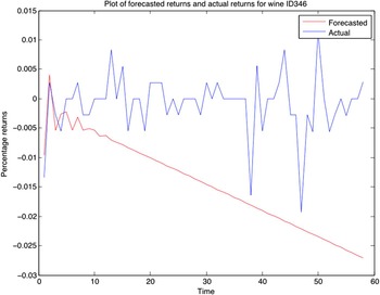
Once again splitting the data into training and test partitions as before and forecasting returns using the GARCH(1,1) model on the first difference, we obtain an average MSE of 4.5 × 10⁻³ which is significantly higher than that of the ARIMA(2,1,1) model. To perhaps understand the reason why this is so, we plot both the forecasted returns and actual returns against time for the forecasted ARIMA(2,1,1) model and the GARCH(1,1) model on the first difference of the returns of wine ID 346 in figures 4 and 5 respectively below. We see that the forecasted returns for the GARCH(1,1) model on the first difference follows closely to the observed returns for the first 10 new test observations but deviates very significantly after that which results in the larger MSE between forecasted returns and actual returns. The forecasted returns for the ARIMA(2,1,1) model, on the other hand, simply predict values closer to the mean of the returns and hence predicts values which on average do not deviate that far from the observed values.
ARIMA(2,1,1) Forecasted vs. Actual Returns of Wine ID 346

GARCH(1,1) Forecasted vs. Actual Returns of Wine ID 346

Finally, we note that a common shortfall of both models as seen from the plots of forecasted vs. actual returns is that the predicted values do not capture the spikes and dips in the actual returns very well. For the ARIMA(2,1,1) model, we simply get a straight line as a prediction and for the GARCH(1,1) model we get a prediction which follows the spikes and dips pretty closely at first, but following that, not only fails to capture the spikes and dips, but also deviates sharply from the trend.
V. Gaussian Process Regression
A. Gaussian Process Theory and Regression
A Gaussian process is a collection of random variables, any finite number of which have a joint Gaussian distribution (Rasmussen and Williams, Reference Rasmussen and Williams2006). A key feature of a Gaussian process is its relationship to linear regression. In particular, we note that Gaussian process regression is essentially equivalent to Bayesian linear regression with an appropriate prior on the weight vector w. Thus given a general learning problem of the form:
 $$y\left( {\bi x} \right) = {\bi \; w}^T \phi \left( {\bi x} \right)$$
where w is an N-dimensional weight vector and φ ( x )is a feature map φ : ℝ n → ℝ N , with N usually ≥ n, and φ ( x ) = [φ 1( x ), φ 2( x ), …, φ N ( x )] where φ i ( x ) are basis functions, that is, non-linear mappings of the input instance x into a higher dimensional feature space. We can place a 0 mean isotropic Gaussian prior with σ 2 I , σ ∈ ℝ over the weight vector w. With this prior over w and integrating, we can rewrite (1) as y( x ) ~ GP (0, σ 2 φ ( x ) T φ ( x′ )) (Bishop, Reference Bishop2006).
Based on what we have done so far, there are two main ways of proceeding with Gaussian process regression on the wine dataset. The first models and forecasts the returns by using a Gaussian process based on ARMA/ARIMA models highlighted in the previous chapter. For the wines in the first group, the returns will be a function of the previous return value since the ARMA(1,1) fitting was found to be ideal for such wines. Thus we have the following model for the wine returns:
 $$Y_t = {\bi w}\phi \left( {Y_{t - 1} + \; \epsilon _t} \right)$$
where φ is some feature map as explained above. For the wines in the second group, the first differenced returns sequence will be a function of the previous two first differenced sequence values based on the optimal ARIMA(2,1,1) fitting. We thus get a model for the first differenced returns sequence of the following form:
 $$D_t = {\bi w}\phi \left( {\bi D} \right) + \; \epsilon _t $$
where D :=
 $$\left[ {\matrix{ {D_{t - 1}} \cr {D_{t - 2}} \cr}} \right]$$
As shown in the beginning of this section, this is equivalent to Gaussian process regression by incorporating a suitable prior on the weight vectors for both cases.
The second way to proceed with Gaussian process regression is to model and forecast the variance of the process by combining Gaussian processes and GARCH models. This is recently seen in the financial literature where Gaussian process and GARCH models are combined to predict stock market volatility with superior performance over the standard GARCH process (Lázaro-Gredilla and Titsias, Reference Lázaro-Gredilla and Titsias2011; Ou and Wang, Reference Ou and Wang2011).
We will only employ the first method in this section and compare the results of this method to the results we obtained in the previous chapter as well as a couple of benchmarks. We ignore the second method mainly because it is focused on volatility forecasting which is not the aim of this project. In addition, we found the ARMA/ARIMA model fitting and forecasting to be much more favorable as compared to GARCH model fitting in the previous section, suggesting that perhaps modeling the conditional variance as a linear function of previous conditional variance terms and the variance of the random process might not be the most suitable for our data.
B. GP-ARMA/GP-ARIMA Regression
Since we observed heavier tails from the residual diagnostics in the previous section, we look at fitting the Laplace likelihood to the data instead of assuming the data comes from a Gaussian distribution. A comparison of the QQplots of the wine returns vs. the quantiles of the standard normal distribution in the case of fitting the Gaussian likelihood to the data, and the quantiles of the exponential distribution in the case of fitting the Laplace likelihood to the data, reveal the Laplace distribution to be a much better fit for almost all of the wines.
In addition, we fit zero-mean Gaussian distribution to the wine returns in the first group and to the differenced returns of the wines in the second group and received average maximal log likelihood values of 141.18 and 222.85 respectively with optimal variance parameters of
 $\sigma _{Gaussian}^2 = 0.05$
for both. Using the Laplace distribution to fit the data, we get higher average maximal log likelihood values of 236.68 and 250.24 respectively, suggesting that the Laplace distribution might be a better fit for for the data. We also obtained average variance parameters of
 $\sigma _{Laplace}^2 = \; 0.01$
for both groups.
We also use various different kernel functions for our Gaussian process regression so as to try and capture the various possible relationships between the wine returns across time. The optimal hyperparameters of the kernels we used for the Gaussian process regression was chosen using cross-validation. Since we note that we seem to be predicting near 0 most of the time, we add the trivial prediction of constantly predicting 0 as one of our benchmarks. Our results are as follows:
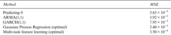
Comparing the MSE scores of the different methods in Tables 1 and 2 we note that we get a lower average MSE value compared to trivially predicting 0 as well as significantly lower values compared to predictions made with the ARMA and GARCH models earlier. This is especially pertinent in the results we get from the wines in the second group. In addition, we look at the Akaike information criterion (AIC) of the different models, which measures the goodness of fit of a model whilst penalizing for excessively complex models (models with too many parameters) and find that for both groups, we can lower AIC values for the optimal Gaussian process regression compared to the ARMA and GARCH models. This again suggests that Gaussian process regression is superior to ARMA and GARCH forecasting for the wines in this category.
Results for Wines in Group 1

Results for Wines in Group 2

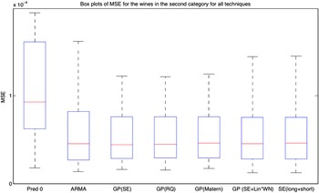
Looking at the boxplots of MSE across all wines in both groups (figures 6 and 7) we observe a persistently smaller whisker range for the Gaussian process regression methods with all the various kernel combinations as compared to the ARMA, GARCH and trivial models. This suggests that we get more consistent results with Gaussian process regression.
Comparing MSE Across all Wines in Group 1 for the Gaussian Process Regression Techniques

Box Plots of MSE Across all Wines in Group 2 for all Techniques (except GARCH)

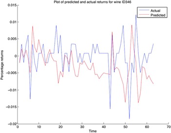
We also compare the plots of predicted vs. actual returns we get from our optimal Gaussian process regression to those from ARMA and GARCH forecasting and find that we seem to learn a more realistic function which better captures how the data varies. Comparing the plots of predicted vs. actual values of wine ID 346 we displayed in figures 4 and 5 earlier and that from Gaussian process regression below in figure 8, we note that unlike the ARMA forecasting which simply predicts a linear function, our optimal Gaussian process prediction of the returns of wine ID 346 as seen in figure 8 actually appears to follow pretty closely to the spikes and dips in the actual returns data. In this sense, we see that the function learned from our optimal Gaussian process model for the wines in this category seems to capture more information and variation in the data.
Predicted vs. Actual returns for wine ID 346

Finally, we compare the results we get from implementing Gaussian process regression on the wines from both categories. From Tables 1 and 2, we note that in general, our algorithms perform better on the wines in category 1 and it certainly seems like the returns of wines from category 1 are easier to predict in general. This is hardly surprising, as we have noted earlier that the wines in category 2 have a more complicated structure and are less similar to one another in general than those in category 1. Nevertheless, we note that interestingly, though Gaussian process regression does give us a better MSE result compared to other techniques like ARMA, GARCH, and even the trivial model of just predicting 0 all the time for the wines in category 1, the improvement in MSE is quite minimal. For the wines in the second category, however, the improvement in MSE of Gaussian process regression over the ARIMA, GARCH, and the trivial model is quite significant. Altogether, this suggests that Gaussian process regression models might perhaps be more suited for the wines in category 2 as it gives us a marked improvement in the overall average MSE for the wines in this category.
VI. Multitask Feature Learning
A. Motivation
A potential problem with our wine data is that the sequence of consistently frequent wine prices only go back to September 2013 (~156 lags long), we do not have as much returns data for each wine we work with. This could result in overfitting in our training data and thus negatively impact our performance on the test data. To address this issue, we use multi-task feature learning which “pools” data across the wines in each group, learning both features common to the wines in each group as well as using these common features to improve price forecasting for each wine.
The basic idea behind multi-task learning is to make use of some measure of task-relatedness and use this relationship between tasks as additional information so as to improve learning for each task in the data-poor environment. We will focus on a feature-centric notion of task-relatedness as developed by Argyriou, Evgeniou, and Pontil in Multi-task Feature Learning (Argyriou et al., Reference Argyriou, Evgeniou, Pontil, Schölkopf, Platt and Hofmann2006) and Convex Multi-task feature learning (Argyriou et al., Reference Argyriou, Evgeniou and Pontil2008), that is, a sequence of tasks can be related in that they all share a common, low-dimensional feature representation. Assuming we know this low-dimensional feature representation of the data, we can re-weight the weight vector in our regression for each task to place more weight on the features in this low-dimensional representation (i.e. the salient features) of the data. In addition, we note that because multi-task feature learning only capitalizes on the related features among tasks to improve learning the individual task functions, we have to use multi-task feature learning in conjunction with other learning algorithms (e.g., ridge regression, SVM regression etc.) to learn the individual task functions. In our case, we will continue using Gaussian process regression to learn the wine returns.
In the simplest example of using multi-task learning for time series forecasting, assuming that the value of the time series at a certain point in time is entirely dependent on previous values, as is most commonly assumed with the ARMA and GARCH models used in most financial time series modeling, and assuming that we do not use a non-linear feature map on the input points, we get the feature space to be the set of previous values for each value of the series. Using multi-task feature learning, this feature space is reduced to a subset of pertinent previous values which might give better predictive results.
B. Results
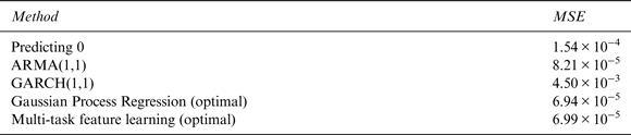
For both groups, the optimal multi-task feature learning algorithm did not perform too well compared to the optimal Gaussian process regression or ARMA/GARCH in terms of MSE as seen from Tables 3 and 6. Upon looking at the plots of predicted returns generated by the multi-task feature learning algorithm, however, we note that we seem to be correctly predicting the direction of change most of the time, but have a difficulty in predicting the magnitude of the change, resulting in our predicted spikes and dips sometimes being much higher or lower than the spikes and dips in the actual series. We see this phenomenon in figures 9 and 10.
Predicted vs. Actual Wine Returns of Wine ID 346

Predicted vs. Actual Wine Returns of Wine ID 8112

MSE Results for Wines in Category 1

Note: Summary of the optimal MSE for wines in category 1 for all methods in terms of predicting the actual wine returns
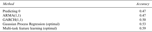
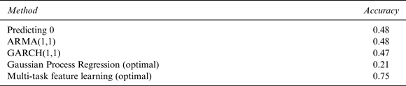
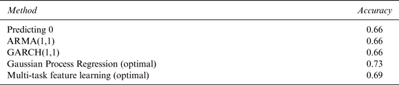
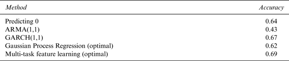
We devised two alternate tests of predictive ability since we feel that though our algorithm underperforms on the wine data in terms of MSE when compared to the other techniques we have tried, our results seem to conform best to the data just from the plots alone. The first test checks if we can perhaps better predict positive or negative wine returns with our algorithm, as measured by the accuracy of our algorithm in predicting the sign of the actual returns series with our predicted series with a 0–1 loss function, instead of focusing on predicting the actual return values. The second checks if we can guess the direction of the change in the actual returns series as measured by predicting the sign of the first difference of the actual returns series with a 0–1 loss function. This corresponds to predicting the sign of the gradient of the actual series. We measure the average accuracy of forecasted prices we get from the previous ARMA/GARCH and Gaussian process regression models using these metrics and the results are shown in Tables 4, 5, 7, and 8.
Accuracy of Predicting the Sign of Wine Returns for Wines in Category 1

Note: Summary of the optimal results for wines in category 1 for all methods in terms of accurately predicting the sign of the actual wine returns
Accuracy of Predicting the Sign of the Change in Wine Returns for Wines in Category 1

Note: Summary of the optimal results for wines in category 1 for all methods in terms of accurately predicting the sign of the change in the actual wine returns
MSE Results for Wines in Category 2

Accuracy of Predicting the sign of Wine Returns for Wines in Category 2

Note: Summary of the optimal results for wines in category 2 for all methods in terms of accurately predicting the sign of the actual wine returns
Accuracy of Predicting the Sign of the Change in Wine Returns for Wines in Category 2

Note: Summary of the optimal results for wines in category 2 for all methods in terms of accurately predicting the sign of the change in the actual wine returns
For the wines in group 1, we obtain the best results from the multi-task learning algorithm when we look at predicting either the sign or the directional change of the actual returns series as seen in figures 4 and 5. This suggests that though our MSE results for our multi-task algorithms might not be as good as those we get from the other methods, including Gaussian process regression, we do seem to learn the signs of the actual returns as well as directional change much better than the other methods. Also, this reinforces our earlier suspicion that perhaps the reason why we get higher MSE results when running our multi-task learning algorithm is due to the fact that the magnitude of our prediction might be wrong, even though we seem to be predicting better in terms of the sign of the returns as well as the directional change.
For the wines in the second group, we note from Tables 7 and 8 that although the multi-task learning algorithm does better than the trivial benchmark and the simple ARMA/GARCH models, the difference in accuracy rate is not as significant as compared to the wines in group 1. In addition, we note that our results from our optimal Gaussian process regression for the wines in this category actually surpasses those obtained from our multi-task algorithm when we look at just predicting the sign of the actual returns. In terms of plots, while we certainly seem to get better plots for our multi-task algorithms, especially compared to that of trivially predicting 0, the simple ARMA/GARCH models as well as Argyriou, Evgeniou, and Pontil's algorithm, we note that the plots we get from our optimal Gaussian process regression as seen in figure 8, are at least as comparable to that we get from our algorithms as seen in figure 9 above. Altogether, this suggests that, for the wines in this category at least, multi-task learning might not be that much more advantageous than Gaussian process regression in terms of predicting either the sign or the directional change of the actual returns series.
VII. Conclusion
Altogether, our results point to the fact that we can draw up two different research problems for the question of best predicting wine prices, each favoring a particular predictive algorithm. The first is more of a regression type of problem and seeks to learn a function which minimizes the difference between the predicted and actual results measured in terms of MSE. The second research problem is classificatory in nature and seeks to learn a function which can most accurately classify the sign of the actual returns as well as accurately classify the direction of the change of the returns series from one point to another.
For the wines in the first group, the first research question favors Gaussian process regression, although the results we get are not much better than that of the simpler ARMA/GARCH prediction techniques, while the second research question favors multi-task learning and we get results which are much better than those we get from the simpler ARMA/GARCH techniques. For the wines in the second group, both research questions favor Gaussian process regression, which gives us results that significantly surpasses those of the simpler models.
A natural consequence of our results is the question: where do we go from here? A well-known theory in finance is the random walk hypothesis, which argues that the prices of stocks evolve according to a random walk and as such cannot be predicted. Consistent with this theory, the best “prediction” we can get measured in terms of MSE is to just predict the empirical mean of the random walk all the time (Lawler, Reference Lawler2010).
Nevertheless our research has shown that, for the 100 wines in the Liv-Ex 100 index at least, this random walk hypothesis does not quite hold. Our superior results with both Gaussian process regression and multi-task learning with regard to both research questions compared to the trivial model of just predicting 0 all the time highlights that there is some pattern we can learn in the wine returns series. In addition, we have also shown that our machine learning techniques give us results with respect to both research questions which are superior to the simpler time series models. Perhaps nowhere is this more evident than in the plots of predicted returns vs. actual returns. Comparing the plots obtained from running our optimal Gaussian process regression and multi-task learning algorithms on the dataset to the ones we get by predicting 0 or just using ARMA/GARCH, we note that our predicted processes manage to capture more of the spikes and dips of the corresponding actual processes compared to that of the simpler models, which suggests that our techniques seem to be capturing more information from the previous return values so as to generate predictions which follow the actual values more closely.
Of course we are aware that we have only been looking at a small subset of wines and that perhaps these 100 Liv-Ex 100 wines just happen to be more predictable than others. Nonetheless, as mentioned in the beginning of this paper, using machine learning techniques in the field of fine wine price prediction is completely unprecedented and our results point to a huge potential of applying more of such machine learning research to the field.