1 Introduction
The unsteady dynamics of a free-surface system driven only by gravity force is encountered in many geophysical applications, such as avalanches, debris flows, lava flows, mudflows, etc. In order to predict the dynamics of these natural flows, several simple configurations have been extensively studied using laboratory experiments, numerical simulations and theoretical descriptions. One of these configurations is the slumping on a horizontal (or inclined) plane of a fluid initially at rest in a reservoir (see figure 1) like a Newtonian fluid (Hoult Reference Hoult1972; Huppert Reference Huppert1982; Stansby, Chegini & Barnes Reference Stansby, Chegini and Barnes1998), a non-Newtonian fluid (Piau & Debiane Reference Piau and Debiane2005; Matson & Hogg Reference Matson and Hogg2007; Balmforth et al. Reference Balmforth, Craster, Perona, Rust and Sassi2007) or even a granular material (Lajeunesse, Monnier & Homsy Reference Lajeunesse, Monnier and Homsy2005; Lube et al. Reference Lube, Huppert, Sparks and Freundt2005).
This configuration can be somewhat related to the case of a gravity current, or even a turbidity current, where the gravity-driven flow is induced by a difference of density between the current and the surrounding fluid (Benjamin Reference Benjamin1968; Hoult Reference Hoult1972; Huppert & Simpson Reference Huppert and Simpson1980; Huppert Reference Huppert1982; Rottman & Simpson Reference Rottman and Simpson1983; Meiburg & Kneller Reference Meiburg and Kneller2010). Whatever the influence of the surrounding fluid is, it is now admitted that the dynamics of such gravity-driven flows are characterized by different regimes, most of which are well predicted by shallow layer/lubrication models. In particular, self-similar solutions can be found depending on the dominant forces in the considered regime. It should be noted that this description disregards the vertical flow which is only dominant at the initial stages of the slumping depending on the initial height of the reservoir.
First, a so-called inertial slumping phase is dominated by inertial effects during which the front velocity remains constant. This regime is similar to the case of a semi-infinite reservoir dam-break problem for which a theoretical prediction of the front evolution was proposed by Ritter (Reference Ritter1892). In this case, dissipation induced by both the boundary layer close to the solid bottom and the bulk turbulence is neglected. The obtained height profile and front position are respectively
 $$\begin{eqnarray}\displaystyle h=\frac{1}{9g}\left(2\sqrt{gH}-\frac{x}{t}\right)^{2},\quad x_{f}=2\sqrt{gH}t, & & \displaystyle\end{eqnarray}$$
where
 $H$
is the initial height of the column and
 $g$
is the gravitational acceleration. Many studies show that this law is hardly reached due to bottom shear dissipation, which becomes significant in regions where the depth of the current becomes small, particularly close to the front (see Dressler Reference Dressler1952; Hogg & Woods Reference Hogg and Woods2001; Hogg & Pritchard Reference Hogg and Pritchard2004, for instance). In this case, the front velocity is shown to remain constant but with a smaller value than Ritter’s prediction. For instance, laboratory experiments (Dressler Reference Dressler1954; Leal, Ferreira & Cardoso Reference Leal, Ferreira and Cardoso2006; Roche et al.
Reference Roche, Montserrat, Niño and Tamburrino2008) and numerical simulations (Bonometti, Balachandar & Magnaudet Reference Bonometti, Balachandar and Magnaudet2008) predict a front velocity that lies in the interval
 $[\sqrt{gH},2\sqrt{gH}]$
, probably depending on the bottom boundary condition. A second inertial regime can be obtained for gravity currents when considering the finite size of the initial reservoir (Hoult Reference Hoult1972; Huppert & Simpson Reference Huppert and Simpson1980). However, in the case of a dam-break flow, i.e. when the surrounding fluid does not influence the dynamics, the front velocity obtained by Ritter (Reference Ritter1892) has been shown to be unaffected by the initial finite length (Hogg Reference Hogg2006).
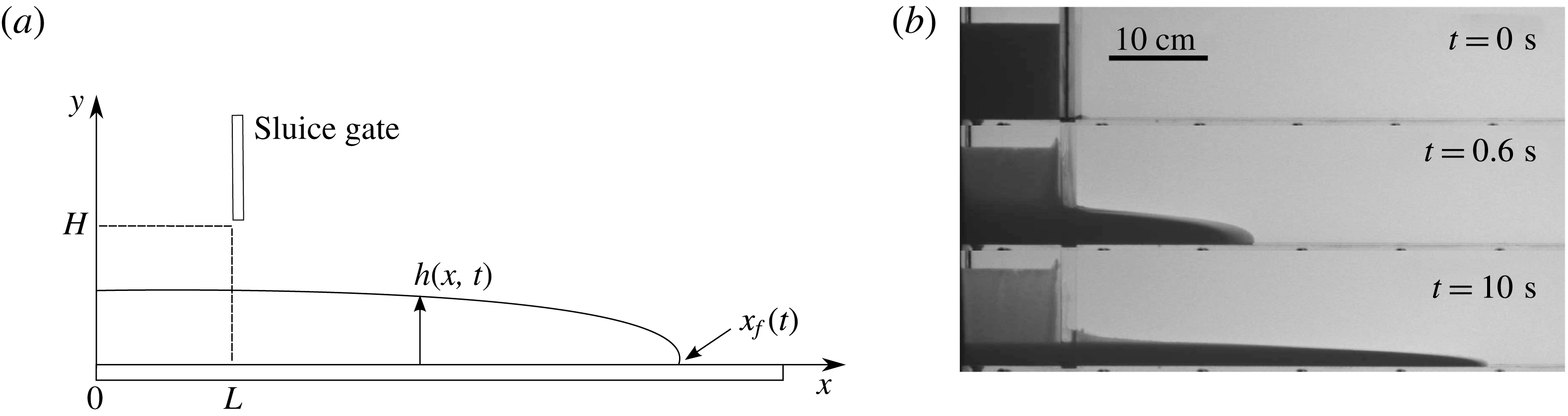
(a) Sketch of the experimental apparatus. (b) Snapshots of the slumping current for
 $\unicode[STIX]{x1D707}_{f}=0.049~\text{Pa}~\text{s}$
,
 $\unicode[STIX]{x1D719}=51.3\,\%$
, particles TS140 and protocol I, at different times.

The final regime is a viscous regime, which is characterized by a balance between gravity and viscous forces. In this case, the solution depends on the rheology of the considered fluid. A self-similar solution can be explicitly derived from lubrication theory in the case of a power-law fluid, for which the shear stress can be written as
 $\unicode[STIX]{x1D70F}=K\dot{\unicode[STIX]{x1D6FE}}^{m}$
, where
 $\dot{\unicode[STIX]{x1D6FE}}$
is the shear rate and
 $K$
and
 $m$
are the consistency and the index of the fluid respectively (Gratton, Minotti & Mahajan Reference Gratton, Minotti and Mahajan1999; Piau & Debiane Reference Piau and Debiane2005; Di Federico, Malavasi & Cintoli Reference Di Federico, Malavasi and Cintoli2006). In particular, the front position is found to be of the form
 $x_{f}\sim t^{m/(2m+3)}$
, as will be recalled in §§ 4 and 5. It can be noted that the Newtonian viscous regime is found for
 $m=1$
, with
 $x_{f}\sim t^{1/5}$
(Huppert Reference Huppert1982). In order to account for the presence of a yield stress observed in some complex fluids, the case of Herschel–Bulkley has also been considered in a few studies (Matson & Hogg Reference Matson and Hogg2007; Balmforth et al.
Reference Balmforth, Craster, Perona, Rust and Sassi2007). However, in this case, the yield stress makes the derivation of a general solution for the evolution of the front position and the height profile more difficult.
In many geophysical applications, the flowing material is a complex combination of different phases which are either fluid or solid. Depending on the considered system, the behaviour of this complex material can then highlight non-Newtonian features such as the ones mentioned above. As often used to highlight the behaviour of such complex materials, the most simple situation of a multiphase system is probably a non-colloidal and neutrally buoyant solid suspension in a Newtonian fluid.
A well-known feature of a neutrally buoyant suspension is the increase of the shear effective viscosity of the material with the volume fraction of the solid phase
 $\unicode[STIX]{x1D719}$
, as explicitly derived by Einstein (Reference Einstein1906) and Batchelor & Green (Reference Batchelor and Green1972) in the case of a relatively small
 $\unicode[STIX]{x1D719}$
. This evolution of the effective viscosity can be attributed to the small-scale interactions between the two phases, which can actually lead to non-Newtonian behaviour due to the local distribution of the particles in the suspension (Batchelor & Green Reference Batchelor and Green1972). These asymptotic models for the effective viscosity at small
 $\unicode[STIX]{x1D719}$
were accurate up to a volume fraction of the order of
 $10\,\%$
(Stickel & Powell Reference Stickel and Powell2005). Only semi-empirical or phenomenological models have been proposed so far to predict the effective viscosity at larger volume fractions. For instance, the Krieger–Dougherty model (Krieger & Dougherty Reference Krieger and Dougherty1959) is one of the most popular and is defined as
 $$\begin{eqnarray}\unicode[STIX]{x1D707}_{eff}=\unicode[STIX]{x1D707}_{f}\left(1-\frac{\unicode[STIX]{x1D719}}{\unicode[STIX]{x1D719}_{m}}\right)^{-\unicode[STIX]{x1D6FC}\unicode[STIX]{x1D719}_{m}},\end{eqnarray}$$
where
 $\unicode[STIX]{x1D719}_{m}$
denotes a maximum volume fraction of the solid phase above which the suspension should be jammed. It can be noted that
 $\unicode[STIX]{x1D6FC}=2.5$
is consistent with Einstein’s model at small
 $\unicode[STIX]{x1D719}$
. However, even if this value of
 $\unicode[STIX]{x1D6FC}$
can be found in the literature (Ovarlez, Bertrand & Rodts Reference Ovarlez, Bertrand and Rodts2006; Huang & Bonn Reference Huang and Bonn2007), a value of
 $\unicode[STIX]{x1D6FC}\unicode[STIX]{x1D719}_{m}=2$
is more widely used to describe experimental results (Ovarlez et al.
Reference Ovarlez, Bertrand and Rodts2006; Mueller, Llewellin & Mader Reference Mueller, Llewellin and Mader2010; Boyer, Guazzelli & Pouliquen Reference Boyer, Guazzelli and Pouliquen2011; Ancey, Andreini & Epely-Chauvin Reference Ancey, Andreini and Epely-Chauvin2013a
; Dbouk, Lobry & Lemaire Reference Dbouk, Lobry and Lemaire2013; Espín & Kumar Reference Espín and Kumar2014a
,Reference Espín and Kumar
b
). The physical origin of this exponent is therefore still not clear. Moreover, the jamming fraction
 $\unicode[STIX]{x1D719}_{m}$
is still under debate in the scientific community, and its value strongly depends on the experimental protocol even when similar materials are used.
The reason for this discrepancy in the evaluation of
 $\unicode[STIX]{x1D719}_{m}$
is often attributed to the small-range interactions between solid particles (Gallier et al.
Reference Gallier, Lemaire, Peters and Lobry2014; Mari et al.
Reference Mari, Seto, Morris and Denn2014). For instance, the solid friction between solid materials, local roughness or air bubbles trapped at the surface of the particles could influence these small-range interactions. However, even if difficult to define, the jamming fraction is usually found in a range of volume fraction
 $\unicode[STIX]{x1D719}_{m}\sim 60\pm 8\,\%$
(Krieger & Dougherty Reference Krieger and Dougherty1959; Nsom Reference Nsom2000; Ovarlez et al.
Reference Ovarlez, Bertrand and Rodts2006; Huang & Bonn Reference Huang and Bonn2007; Bonnoit et al.
Reference Bonnoit, Darnige, Clement and Lindner2010; Mueller et al.
Reference Mueller, Llewellin and Mader2010; Boyer et al.
Reference Boyer, Guazzelli and Pouliquen2011; Dbouk et al.
Reference Dbouk, Lobry and Lemaire2013; Mari et al.
Reference Mari, Seto, Morris and Denn2014).
Beyond the
 $\unicode[STIX]{x1D719}$
dependence of the effective viscosity, neutrally buoyant suspensions have been shown to highlight non-Newtonian behaviour such as shear-thickening/-thinning, yield stress, normal stress differences, etc. in many configurations (Gadala-Maria & Acrivos Reference Gadala-Maria and Acrivos1980; Leighton & Acrivos Reference Leighton and Acrivos1987; Lyon & Leal Reference Lyon and Leal1998; Snabre & Pouligny Reference Snabre and Pouligny2008; Fall et al.
Reference Fall, Bertrand, Ovarlez and Bonn2009, Reference Fall, Lemaitre, Bertrand, Bonn and Ovarlez2010; Ancey et al.
Reference Ancey, Andreini and Epely-Chauvin2013a
; Andreini, Ancey & Epely-Chauvin Reference Andreini, Ancey and Epely-Chauvin2013; Espín & Kumar Reference Espín and Kumar2014a
). Even if the origin of these mechanisms is not always obvious, it is clear that migration processes of the solid phase can play a significant role in the apparent behaviour of the suspension at the scale of the considered system, as the material becomes heterogeneous. Migration is generally attributed to a velocity gradient within the suspension or collisions at high volume fraction leading to a particle flux from high to low shear rates (Lhuillier Reference Lhuillier2009). In fact, any force applied to the particles that induces a modification of the local volume fraction can lead to this migration, inducing apparent non-Newtonian behaviour (Huang et al.
Reference Huang, Ovarlez, Bertrand, Rodts, Coussot and Bonn2005; Ovarlez et al.
Reference Ovarlez, Bertrand and Rodts2006; Fall et al.
Reference Fall, Bertrand, Ovarlez and Bonn2009; Andreini et al.
Reference Andreini, Ancey and Epely-Chauvin2013). The role of the migration of particles within the suspension would then be to modify the local volume fraction, the apparent fluid becoming non-homogeneous and highlighting an apparent non-Newtonian behaviour at the scale of the studied system.
Beyond this migration process or local heterogeneities, apparent non-Newtonian behaviour could be also discussed in terms of a transition based on the local dynamics of the particles within the suspension (Bagnold Reference Bagnold1954; Fall et al.
Reference Fall, Lemaitre, Bertrand, Bonn and Ovarlez2010; Trulsson, Andreotti & Claudin Reference Trulsson, Andreotti and Claudin2012). For a given volume fraction
 $\unicode[STIX]{x1D719}$
, this transition delimits a viscous Newtonian regime, characterized by a constant effective viscosity, from a Bagnold type regime, for which the shear stress to shear rate relationship becomes quadratic, depending on the relative influence of the viscous dissipation at the scale of the particle and its inertia (Fall et al.
Reference Fall, Lemaitre, Bertrand, Bonn and Ovarlez2010). This transition is usually found to be a function of the local shear rate
 $\dot{\unicode[STIX]{x1D6FE}}$
and the volume fraction
 $\unicode[STIX]{x1D719}$
through the Bagnold number
 $Ba$
(Bagnold Reference Bagnold1954). This dimensionless number is defined as
 $Ba=f(\unicode[STIX]{x1D719})Re_{p}$
, where
 $f(\unicode[STIX]{x1D719})$
is a
 $\unicode[STIX]{x1D719}$
-dependent function equal to
 $f(\unicode[STIX]{x1D719})=[(0.74/\unicode[STIX]{x1D719})^{1/3}-1]^{-1/2}$
(Bagnold Reference Bagnold1954), even if other expressions can be also found in the literature (Fall et al.
Reference Fall, Lemaitre, Bertrand, Bonn and Ovarlez2010; Trulsson et al.
Reference Trulsson, Andreotti and Claudin2012), and
 $Re_{p}=\unicode[STIX]{x1D70C}d^{2}\dot{\unicode[STIX]{x1D6FE}}/\unicode[STIX]{x1D707}_{f}$
is the particle Reynolds number. However, the transition from viscous to particle-inertial regimes is still unclear and the Bagnold number can be found in the range
 $Ba\sim 10^{-2}{-}10^{3}$
in the literature, and some of these observations are still debated (Hunt et al.
Reference Hunt, Zenit, Campbell and Brennen2002). In any case, the microscale dynamics, i.e. the dynamics at the scale of the particle, plays a significant role in the dynamics of neutrally buoyant suspensions, which could therefore strongly alter the dynamics of unsteady flows.
In the present study, the dam-break of a neutrally buoyant suspension over a horizontal bottom in a rectangular geometry is considered. Gravity-driven flows of a non-colloidal and neutrally buoyant suspension have been investigated in some studies (see Nsom Reference Nsom2000; Ward et al. Reference Ward, Wey, Glidden, Hosoi and Bertozzi2009; Bonnoit et al. Reference Bonnoit, Darnige, Clement and Lindner2010; Ancey et al. Reference Ancey, Andreini and Epely-Chauvin2013a ; Ancey, Andreini & Epely-Chauvin Reference Ancey, Andreini and Epely-Chauvin2013b ; Andreini et al. Reference Andreini, Ancey and Epely-Chauvin2013, for instance). Nevertheless, the study of the suspension flow on an inclined plane, with specific attention paid to the steady state, is more often considered and, to the best of our knowledge, only one article has considered the unsteady dynamics of slumping on a horizontal plane (Nsom Reference Nsom2000). Here, the focus is made on the description of the flow dynamics and the extraction of rheological behaviour, either Newtonian or non-Newtonian, at the scale of the current through the time evolution of the front position. It should be noted that a similar procedure was used by Castruccio, Rust & Sparks (Reference Castruccio, Rust and Sparks2010) in the case of suspensions of cubic crystals in various viscous liquids. In view of the previous studies on the dynamics of a slumping fluid and the rheology of a neutrally buoyant suspension, the key questions to be addressed in the following paper are as follows. (i) Are the different regimes observed in previous studies for the case of a single-phase Newtonian fluid slumping over a horizontal bottom still observed in the case of a neutrally buoyant suspension? (ii) Are the models of effective shear viscosity pertinent according to the self-similar viscous solution of a slumping current? (iii) How do apparent non-Newtonian behaviours manifest themselves on the dynamics of the current?
This paper is organized as follows. In § 2, we present the experimental set-up. Then, we show results obtained in the constant-speed inertial regime (§ 3) and in the viscous Newtonian regime (§ 4). Finally, in § 5, we present some apparent non-Newtonian behaviours (shear-thinning, shear-thickening, yielding) observed in our experiments on a longer time scale in the viscous-dominated regime.
2 Experimental set-up
2.1 Dam-break apparatus
In this study, experiments are conducted in a horizontal transparent channel of rectangular cross-section. The channel is
 $2~\text{m}$
long,
 $0.35~\text{m}$
high and
 $0.20~\text{m}$
wide along the streamwise
 $x$
, vertical
 $y$
and spanwise
 $z$
coordinates respectively (see figure 1
a). On one side of the channel,
 $x=0$
, a finite volume reservoir is delimited by a sluice gate positioned at
 $x=L=10~\text{cm}$
. In this study, the initial height of fluid
 $H$
in the reservoir is set constant,
 $H=10~\text{cm}$
. The aspect ratio of the initial column is then
 $a=H/L=1$
. At time
 $t=0$
, the manual sluice gate is removed in approximately
 $0.1~\text{s}$
and the fluid is released. The height profile
 $h(x,t)$
is extracted from image analysis using a classical shadowgraphy method. For this purpose, the 2D flow in the
 $(x,y)$
plane is recorded using two sCMOS Lavision
 $2560\times 2160$
pixel cameras and a backlight source on the opposite side of the channel. The acquisition rate of the cameras is varied from
 $10$
Hz to
 $200$
Hz depending on the time scale of the slumping dynamics. The obtained resolution is approximately
 $500~\unicode[STIX]{x03BC}\text{m}~\text{pix}^{-1}$
, allowing heights down to
 $1$
mm to be captured. The extraction process is performed using a Matlab routine.
2.2 Neutrally buoyant suspension
For all experiments, a mixture of water and Ucon oil 75H90000 (a viscous Newtonian fluid soluble in water) is used as the Newtonian interstitial fluid of viscosity
 $\unicode[STIX]{x1D707}_{f}$
and density
 $\unicode[STIX]{x1D70C}$
. The relative concentration of Ucon oil and water is characterized by the mass fraction
 $c_{m}=m_{o}/(m_{o}+m_{w})$
, with
 $m_{o}$
and
 $m_{w}$
the mass of oil and water respectively. The mass fraction
 $c_{m}$
is varied from
 $0\,\%$
(pure water) to
 $73.2\,\%$
, which corresponds to a variation of viscosity in the range
 $\unicode[STIX]{x1D707}_{f}=[10^{-3},10]~\text{Pa}~\text{s}$
. Sodium chloride (NaCl) is added to the fluid mixture to match the suspended particle density. The density of the interstitial fluid is measured by a DMA 35 Anton Paar electronic densimeter with an accuracy of
 $\pm 0.5~\text{kg}~\text{m}^{-3}$
. Finally, the viscosity is measured using a cone-plate geometry in a Haake Mars III rheometer with an accuracy of less than
 $5\,\%$
.
The particles used are monodisperse spherical polystyrene beads manufactured by Microbeads AS. Particles of diameter
 $d=41.8\pm 0.9~\unicode[STIX]{x03BC}\text{m}$
,
 $d=80.7\pm 7.3~\unicode[STIX]{x03BC}\text{m}$
,
 $d=141.8\pm 3.1~\unicode[STIX]{x03BC}\text{m}$
and
 $d=228\pm 7~\unicode[STIX]{x03BC}\text{m}$
, referred to as TS40, TS80, TS140 and TS250 respectively in the following, are used. In order to measure particle mean densities and dispersion, a sample of particles is poured into a tank filled with linearly density stratified salty water. The initial concentration of particles is lower than
 $0.5\,\%$
during the slow settling of the particles in the stratified fluid to prevent any collective effects. Once the particles are at rest, their mean height level in the tank gives the mean density while their vertical spreading indicates the dispersion in density. The obtained mean density is double-checked using several samples of fluid of constant density, whose density ranges from
 $1045~\text{kg}~\text{m}^{-3}$
to
 $1065~\text{kg}~\text{m}^{-3}$
with a difference of
 $1~\text{kg}~\text{m}^{-3}$
. After several hours, the sample with particles remaining in the bulk, not settling or creaming, indicates the density of particles. The obtained densities are
 $1050~\text{kg}~\text{m}^{-3}$
,
 $1060~\text{kg}~\text{m}^{-3}$
,
 $1060~\text{kg}~\text{m}^{-3}$
and
 $1063~\text{kg}~\text{m}^{-3}$
for TS40, TS80, TS140 and TS250 respectively, with a dispersion of
 $\pm 2~\text{kg}~\text{m}^{-3}$
. The overall error in density matching between the particles and the interstitial fluid can only be attributed to the particle density dispersion and is therefore of the order of
 $\pm 2~\text{kg}~\text{m}^{-3}$
. It should be noted that to confirm the results discussed in the following, several experiments were performed with density mismatch from
 $-10~\text{kg}~\text{m}^{-3}$
to
 $+10~\text{kg}~\text{m}^{-3}$
, i.e. well above the density uncertainty, to exclude any density effects from the physical analysis (not shown here). The volume fraction
 $\unicode[STIX]{x1D719}$
of the suspension is the same as the measured mass fraction
 $\unicode[STIX]{x1D719}_{weight}$
as the suspension is density matched. The volume fraction
 $\unicode[STIX]{x1D719}$
is then simply obtained from the mass of dry particles
 $m_{p}$
and the total mass
 $m_{t}$
as
 $\unicode[STIX]{x1D719}=\unicode[STIX]{x1D719}_{weight}=m_{p}/m_{t}$
.
Two different procedures are used to prepare the suspension, which will be referred to in the following as protocol I and protocol II. In protocol I, particles are mixed with the interstitial fluid, while in protocol II, Triton X-100 is added to the solution to prevent particle aggregation from air entrainment trapped at the particle surface. The concentration of Triton X-100 varies with the total apparent surface of solid particles in the suspension, i.e. the critical micelle concentration (CMC), which depends on the size and volume fraction of particles. Here,
 $0.5~\text{mL}$
of Triton X-100 is used for an equivalent solid surface of
 $90~\text{m}^{2}$
. In both protocols, the suspension is stirred for several hours (up to 24 h). It should be noted that, as for uncertainties in density mismatch, several experiments have been performed with different concentrations of Triton X-100 to exclude any misinterpretation due to any influence of this solvent (not shown here).
An example of a typical suspension slumping in the channel is shown at three different times in figure 1(b). See also movies 1 and 2 available online at https://doi.org/10.1017/jfm.2017.471. The different regimes observed in the dynamics of such a current are discussed in the following.
2.3 Dimensionless parameters
Different dimensionless numbers can be defined for this configuration. In this section, we discuss the order of magnitude of these different numbers to anticipate their relative influence on the dynamics. Beyond the initial length scales, which are
 $H=10~\text{cm}$
and
 $L=10~\text{cm}$
for the height and horizontal length respectively, the characteristic height
 $h$
and length
 $l$
of the current during a typical experiment are also used and are estimated to be of the order of
 $h\sim H/10=1~\text{cm}$
and
 $l\sim 1~\text{m}$
in our experiments. The aspect ratio of the current thus satisfies
 $h/l\sim 0.1$
.
At the scale of the current, the Reynolds number
 $Re=\unicode[STIX]{x1D70C}Uh/\unicode[STIX]{x1D707}$
, with
 $U=\sqrt{gh}$
the velocity scale, is in the range
 $Re=[10^{-1},10^{3}]$
in our study. The dynamic viscosity
 $\unicode[STIX]{x1D707}$
is chosen as
 $\unicode[STIX]{x1D707}=\unicode[STIX]{x1D707}_{f}$
for Newtonian single-phase currents and
 $\unicode[STIX]{x1D707}=\unicode[STIX]{x1D707}_{eff}$
for the suspension currents. The value of
 $\unicode[STIX]{x1D707}_{eff}$
can be estimated from available data in the literature or a posteriori in the present study. This large Reynolds number range allows us to study inertial and viscous macroscopic dynamics, at least for small to moderate
 $\unicode[STIX]{x1D707}_{f}$
and
 $\unicode[STIX]{x1D719}$
. The Bond number, based on the initial height
 $H$
, and defined as
 $Bo=\unicode[STIX]{x1D70C}gH^{2}/\unicode[STIX]{x1D70E}$
, with
 $\unicode[STIX]{x1D70E}$
the surface tension, is found to be
 $Bo\sim 10^{3}\gg 1$
, which suggests that capillarity effects are negligible on the initial column. It should be noted that to confirm that capillarity does not influence the dynamics of the current in the viscous-dominated regime, the capillarity number which compares viscous effects with surface tension at the front scale
 $Ca=U_{v}\unicode[STIX]{x1D707}/\unicode[STIX]{x1D70E}$
, with
 $U_{v}=\unicode[STIX]{x1D70C}gh^{2}/\unicode[STIX]{x1D707}$
, can be estimated as
 $Ca\sim 10$
, i.e. larger than
 $1$
.
At the scale of the particle, the Peclet number
 $Pe=6\unicode[STIX]{x03C0}\unicode[STIX]{x1D707}a^{3}\dot{\unicode[STIX]{x1D6FE}}/kT$
is found to satisfy
 $Pe\gg 1$
, leading to no influence of Brownian motion. Moreover, the particle Reynolds number
 $Re_{p}=\unicode[STIX]{x1D70C}d^{2}\dot{\unicode[STIX]{x1D6FE}}/\unicode[STIX]{x1D707}_{f}$
is found to be in the range of
 $Re_{p}=[10^{-3},1]$
. According to Stickel & Powell (Reference Stickel and Powell2005),
 $Re_{p}$
cannot be neglected and could play a significant role in the transition from viscous to particle-inertia regimes according to the Bagnold transition mentioned in § 1. This transition is usually defined as a function of
 $f(\unicode[STIX]{x1D719})Re_{p}$
, where different functions
 $f(\unicode[STIX]{x1D719})$
are found in the literature. It should be noted that
 $f(\unicode[STIX]{x1D719})=\unicode[STIX]{x1D706}^{1/2}=[(0.74/\unicode[STIX]{x1D719})^{1/3}-1]^{-1/2}$
leads to the well-known Bagnold number
 $Ba=\unicode[STIX]{x1D706}^{1/2}Re_{p}$
. In our case, the Bagnold number is in the range of
 $Ba=[10^{-3},10]$
, which suggests a possible transition between these regimes.
3 Inertial slumping regime and transition
The collapse of a Newtonian fluid column can exhibit an inertial constant-speed slumping phase at the first stages of the propagation, at least when the fluid viscosity is small enough. Here, we define the inertial dimensionless variables as
 $$\begin{eqnarray}h^{I}=\frac{h}{H},\quad x^{I}=\frac{x-L}{H},\quad t^{I}=\frac{\sqrt{gH}}{H}t.\end{eqnarray}$$
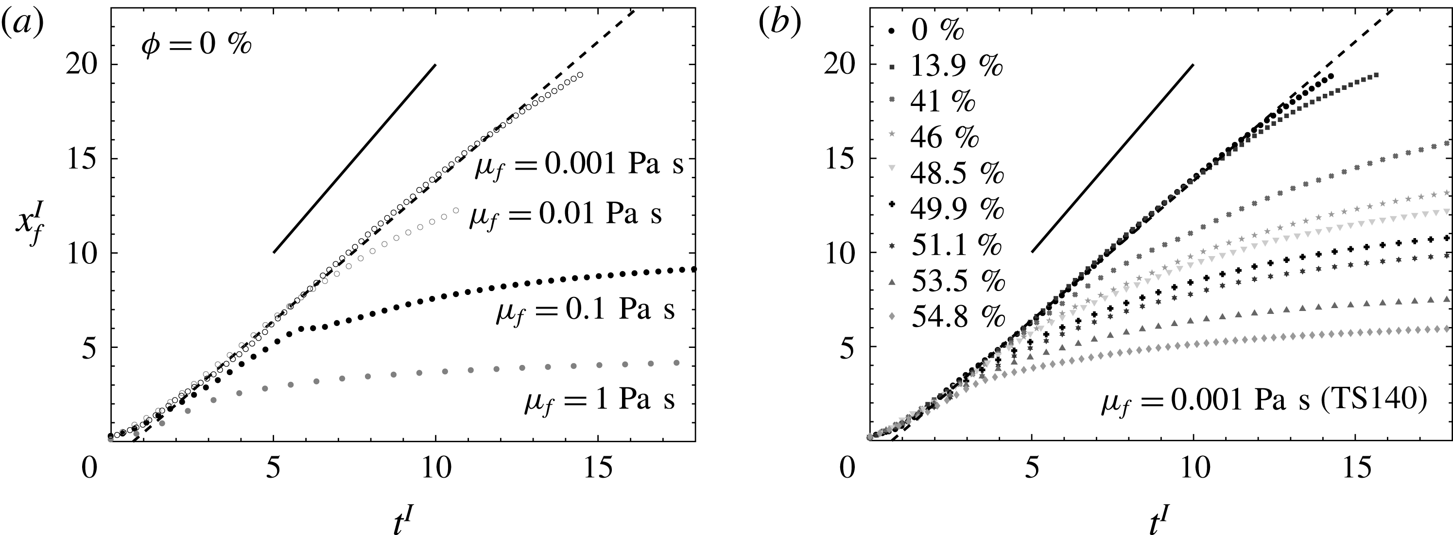
Figure 2 shows the front position
 $x_{f}^{I}$
as a function of
 $t^{I}$
for
 $\unicode[STIX]{x1D719}=0$
and
 $\unicode[STIX]{x1D707}_{f}=[10^{-3},10^{-2},10^{-1},1]~\text{Pa}~\text{s}$
(a) and for
 $\unicode[STIX]{x1D707}_{f}=10^{-3}~\text{Pa}~\text{s}$
and
 $\unicode[STIX]{x1D719}\in [0,0.548]$
(b). It should be noted that figure 2(a) corresponds to the Newtonian single-phase fluids. It can be observed that the single-phase fluids (a) and suspensions (b) highlight a similar trend. In particular, the constant-velocity phase corresponding to the inertial slumping regime is obtained in both configurations after an acceleration phase which ends at around
 $t^{I}\approx 2$
. It should be noted that this acceleration phase corresponds to a conversion from the initial potential energy to the horizontal kinetic energy, involving vertical acceleration, as mentioned in § 1. The acceleration phase is not discussed in the following. It should be noted also that the inertial slumping regime is observed in our set of experiments only for
 $Re\gtrsim 1$
. Otherwise, the currents evolve from the acceleration towards the viscous-dominated regime. In the inertial slumping regime, i.e.
 $t^{I}>2$
, the obtained constant front velocity is in accordance with Ritter’s prediction,
 $2\sqrt{gH}$
(see (1.1)), i.e.
 $x_{f}^{I}=2t^{I}$
in dimensionless form (solid line in figure 2). As shown in figure 2, Ritter’s solution slightly overestimates the front velocity obtained in the experiments, and a better approximation is shown here to be
 $1.5\sqrt{gH}$
, i.e.
 $x_{f}^{I}=1.5t^{I}$
(dashed line in figure 2). As discussed in § 1, this difference between the theoretical prediction and the experiments is in agreement with results obtained in the literature (Dressler Reference Dressler1954; Leal et al.
Reference Leal, Ferreira and Cardoso2006; Roche et al.
Reference Roche, Montserrat, Niño and Tamburrino2008), in which the discrepancy was attributed to the basal drag close to the bottom plane that is not taken into account in the theoretical prediction. In particular, the dissipation is usually found to be dominant close to the front. In order to estimate the length on which most of the dissipation occurs, Hogg & Pritchard (Reference Hogg and Pritchard2004) showed that friction is significant when
 $\unicode[STIX]{x1D709}=x_{f}-x\lesssim (C_{D}g^{2}Ht^{4})^{1/3}$
, where
 $C_{D}$
is the drag coefficient and
 $H$
is the initial height. The drag coefficient can be defined as
 $C_{D}=0.025Re_{H}^{-0.2}$
, where the Reynolds number is defined as
 $Re_{H}=\unicode[STIX]{x1D70C}\sqrt{gH^{3}}/\unicode[STIX]{x1D707}$
(Hager Reference Hager1988). In our case, this estimation gives that
 $\unicode[STIX]{x1D709}$
is approximately
 $15\,\%$
of the length
 $x_{f}$
on the time scale of the constant-speed inertial regime.
Evolution of the front position
 $x_{f}^{I}$
as a function of time
 $t^{I}$
in inertial dimensionless form (3.1) for Newtonian single-phase fluids with various values of
 $\unicode[STIX]{x1D707}_{f}$
(a) and suspensions with various values of
 $\unicode[STIX]{x1D719}$
(b). The suspensions are composed of particles TS140 and
 $\unicode[STIX]{x1D707}_{f}=10^{-3}~\text{Pa}~\text{s}$
using protocol I. The solid line (——) is Ritter’s solution (
 $x_{f}^{I}=2t^{I}$
) and the dashed line (- - -) is the best fit (
 $x_{f}^{I}=1.5t^{I}$
).

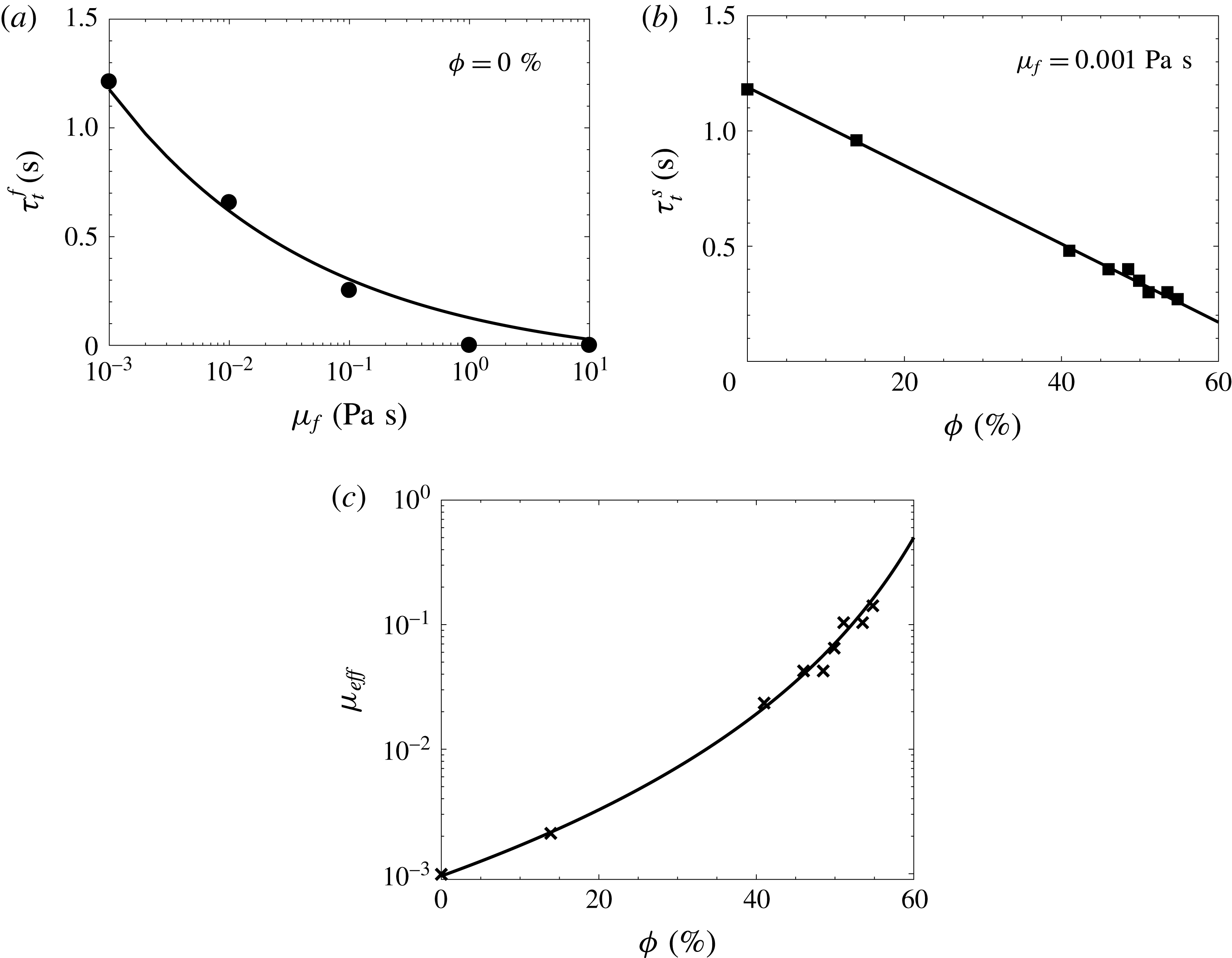
(a) The transition time
 $\unicode[STIX]{x1D70F}_{t}^{f}$
as a function of the viscosity
 $\unicode[STIX]{x1D707}_{f}$
for Newtonian single-phase currents (
 $\unicode[STIX]{x1D719}=0$
). The solid line (——) corresponds to the theoretical prediction (see text) with a slight offset, i.e.
 $\unicode[STIX]{x1D70F}_{t}^{f}=0.227\unicode[STIX]{x1D707}_{f}^{-1/4}-0.1$
. (b) The transition time
 $\unicode[STIX]{x1D70F}_{t}^{s}$
as a function of the volume fraction
 $\unicode[STIX]{x1D719}$
for suspension currents with
 $\unicode[STIX]{x1D707}_{f}=0.001~\text{Pa}~\text{s}$
. The solid line (——) represents the best linear fit,
 $\unicode[STIX]{x1D70F}_{t}^{s}=-1.7\unicode[STIX]{x1D719}+1.19$
. (c) The effective viscosity
 $\unicode[STIX]{x1D707}_{eff}$
as a function of the volume fraction
 $\unicode[STIX]{x1D719}$
. The crosses correspond to
 $\unicode[STIX]{x1D707}_{eff}=((\unicode[STIX]{x1D70F}_{t}^{s}+0.1)/0.227)^{-4}$
, with
 $\unicode[STIX]{x1D70F}_{t}^{s}$
corresponding to the experimental estimation (squares in figure 3
b), while the solid line is
 $\unicode[STIX]{x1D707}_{eff}=\unicode[STIX]{x1D6FD}(1-\unicode[STIX]{x1D719}/\unicode[STIX]{x1D719}_{m})^{-\unicode[STIX]{x1D6FC}\unicode[STIX]{x1D719}_{m}}$
with
 $\unicode[STIX]{x1D719}_{m}\sim 76\,\%$
,
 $\unicode[STIX]{x1D6FC}\sim 5.3$
and
 $\unicode[STIX]{x1D6FD}=0.96\times 10^{-3}~\text{Pa}~\text{s}$
.

After the slumping phase, the front velocity decreases. This indicates the transition from the inertial regime towards a viscous-dominated regime. We define the transition time
 $\unicode[STIX]{x1D70F}_{t}$
as the time at which the front position deviates from the best fit solution
 $x_{f}^{I}=1.5t^{I}$
(dashed line on the figure 2), suggesting the end of the inertial slumping regime.
From figure 2(a), one can therefore extract a transition time referred to as
 $\unicode[STIX]{x1D70F}_{t}^{f}$
which only depends on
 $\unicode[STIX]{x1D707}_{f}$
at
 $\unicode[STIX]{x1D719}=0$
. This transition time
 $\unicode[STIX]{x1D70F}_{t}^{f}$
is shown as a function of
 $\unicode[STIX]{x1D707}_{f}$
in figure 3(a). It should be noted that for
 $\unicode[STIX]{x1D707}_{f}>1~\text{Pa}~\text{s}$
, no inertial slumping is observed and the dynamics of the front is only controlled by viscous effects after the acceleration phase. The transition time
 $\unicode[STIX]{x1D70F}_{t}^{f}$
thus falls down to zero in this case. The evolution of the transition time
 $\unicode[STIX]{x1D70F}_{t}^{f}$
as a function of the viscosity
 $\unicode[STIX]{x1D707}_{f}$
can be estimated by equalizing the spreading laws obtained in both the inertial and viscous regimes (Amy et al.
Reference Amy, Hogg, Peakall and Talling2005). In the inertial regime, the front position was found to follow the law
 $x_{f}=1.5(gH)^{1/2}t$
, while the front position can be defined as
 $x_{f}=\unicode[STIX]{x1D702}_{n}(\unicode[STIX]{x1D70C}g(HL)^{3}t/3\unicode[STIX]{x1D707}_{f})^{1/5}$
in the viscous regime, from the self-similar solution recalled in § 1. Considering that these solutions merge at
 $\unicode[STIX]{x1D70F}_{t}^{f}$
, this leads to
 $\unicode[STIX]{x1D70F}_{t}^{f}=0.227\unicode[STIX]{x1D707}_{f}^{-1/4}$
. (It should be noted that the constants obtained from fitting analysis in this section are dimensional. Their dimension is not reported for the sake of simplicity as it can be easily obtained.) As shown in figure 3, this solution is in very good agreement with the experimental data, accounting for a slight offset such as
 $\unicode[STIX]{x1D70F}_{t}^{f}=0.227\unicode[STIX]{x1D707}_{f}^{-1/4}-0.1$
(see the solid line in figure 3
a).
From figure 2(b), a transition time
 $\unicode[STIX]{x1D70F}_{t}^{s}$
can be obtained as a function of
 $\unicode[STIX]{x1D719}$
at
 $\unicode[STIX]{x1D707}_{f}=10^{-3}~\text{Pa}~\text{s}$
. In figure 3(b),
 $\unicode[STIX]{x1D70F}_{t}^{s}$
is plotted as a function of
 $\unicode[STIX]{x1D719}$
, and it is shown to decrease linearly with
 $\unicode[STIX]{x1D719}$
, as
 $\unicode[STIX]{x1D70F}_{t}^{s}=-1.7\unicode[STIX]{x1D719}+1.19$
(solid line in figure 3
b). One can then define the effective viscosity of the suspension
 $\unicode[STIX]{x1D707}_{eff}$
as the fluid viscosity that allows the two transition times
 $\unicode[STIX]{x1D70F}_{t}^{f}$
and
 $\unicode[STIX]{x1D70F}_{t}^{f}$
to be balanced. In other words,
 $\unicode[STIX]{x1D707}_{eff}$
is such that
 $\unicode[STIX]{x1D70F}_{t}^{f}=\unicode[STIX]{x1D70F}_{t}^{s}$
, i.e.
 $0.227\unicode[STIX]{x1D707}_{eff}^{-1/4}-0.1=\unicode[STIX]{x1D70F}_{t}^{s}$
. The obtained results for
 $\unicode[STIX]{x1D707}_{eff}$
are plotted as a function of
 $\unicode[STIX]{x1D719}$
in figure 3(c). In this figure, the symbols correspond to
 $\unicode[STIX]{x1D707}_{eff}=((\unicode[STIX]{x1D70F}_{t}^{s}+0.1)/0.227)^{-4}$
, where the actual measure of
 $\unicode[STIX]{x1D70F}_{t}^{s}$
is used, while the solid line is the solution of
 $0.227\unicode[STIX]{x1D707}_{eff}^{-1/4}-0.1=-1.7\unicode[STIX]{x1D719}+1.19$
. The obtained scaling is in good agreement with the data and the associated effective viscosity resembles the Krieger–Dougherty model (1.2), as it can be rewritten as
 $\unicode[STIX]{x1D707}_{eff}=\unicode[STIX]{x1D6FD}(1-\unicode[STIX]{x1D719}/\unicode[STIX]{x1D719}_{m})^{-\unicode[STIX]{x1D6FC}\unicode[STIX]{x1D719}_{m}}$
, with
 $\unicode[STIX]{x1D719}_{m}\sim 76\,\%$
,
 $\unicode[STIX]{x1D6FC}\sim 5.3$
and
 $\unicode[STIX]{x1D6FD}=0.96\times 10^{-3}~\text{Pa}~\text{s}$
(solid line in figure 3
c). Given the gross estimation of
 $\unicode[STIX]{x1D707}_{eff}$
, through the determination of transition times, the obtained values are surprisingly of the expected order of magnitude. In particular, it should be noted that the value of
 $\unicode[STIX]{x1D6FD}=0.96\times 10^{-3}~\text{Pa}~\text{s}$
, which results from measurements and scaling law fittings, should represent the fluid viscosity at
 $\unicode[STIX]{x1D719}=0$
for this solution. Indeed, this is in good agreement with the interstitial fluid used for the suspension case, i.e. water with a viscosity of
 $10^{-3}~\text{Pa}~\text{s}$
.
4 Apparent Newtonian viscous regime
In this section, we focus on the viscous regime. After the transition
 $\unicode[STIX]{x1D70F}_{t}$
mentioned in the previous section, the dynamics of the front then evolves towards a viscous regime.
As long as the suspension can be considered as a viscous Newtonian fluid, the effective viscosity
 $\unicode[STIX]{x1D707}_{eff}$
is the pertinent parameter that controls the dynamics of the current in the viscous regime. This assumption is in accordance with the previously obtained effective viscosity from the transition time scales.
In the viscous regime, a more accurate estimation of this effective viscosity can be expected. For this purpose, the self-similar solution for a viscous Newtonian fluid (i.e.
 $m=1$
) and given by Huppert (Reference Huppert1982) is detailed here. In particular, the evolution of the front position and the height profile is obtained as a self-similar solution using lubrication theory, far from the initial condition, and will be referred to in the following as
 $x_{f}^{(s)}$
and
 $h^{(s)}$
. The solution for a two-dimensional planar collapse in the viscous regime reads
 $$\begin{eqnarray}\displaystyle & \displaystyle x_{f}^{(s)}(t)=\unicode[STIX]{x1D702}_{n}\left(\frac{\unicode[STIX]{x1D70C}gA^{3}}{3\unicode[STIX]{x1D707}_{eff}}t\right)^{1/5}, & \displaystyle\end{eqnarray}$$
 $$\begin{eqnarray}\displaystyle & \displaystyle h^{(s)}(x,t)=\unicode[STIX]{x1D702}_{n}^{2/3}\left(\frac{3A^{2}\unicode[STIX]{x1D707}_{eff}}{\unicode[STIX]{x1D70C}g}\right)^{1/5}t^{-1/5}f(x/x_{f}^{(s)}), & \displaystyle\end{eqnarray}$$
where
 $\unicode[STIX]{x1D702}_{n}\sim 1.411$
is a constant,
 $A=HL$
is the area of the slumping material and
 $f(x/x_{f}^{(s)})=(3/10)^{1/3}(1-(x/x_{f}^{(s)})^{2})^{1/3}$
for a horizontal channel.
In order to estimate
 $\unicode[STIX]{x1D707}_{eff}$
from the experimental measurement of the front position
 $x_{f}$
in the viscous regime, we therefore define
 $X_{f}=(x_{f}/\unicode[STIX]{x1D702}_{n})^{5}$
, which should be a linear function of
 $t$
according to (4.1). Then, the effective viscosity is simply determined from the front position as
 $$\begin{eqnarray}\unicode[STIX]{x1D707}_{eff}=\frac{\unicode[STIX]{x1D70C}gA^{3}}{3}\left(\frac{\text{d}X_{f}}{\text{d}t}\right)^{-1}.\end{eqnarray}$$
It should be noted that this definition allows us to overcome the problem of time offsets.
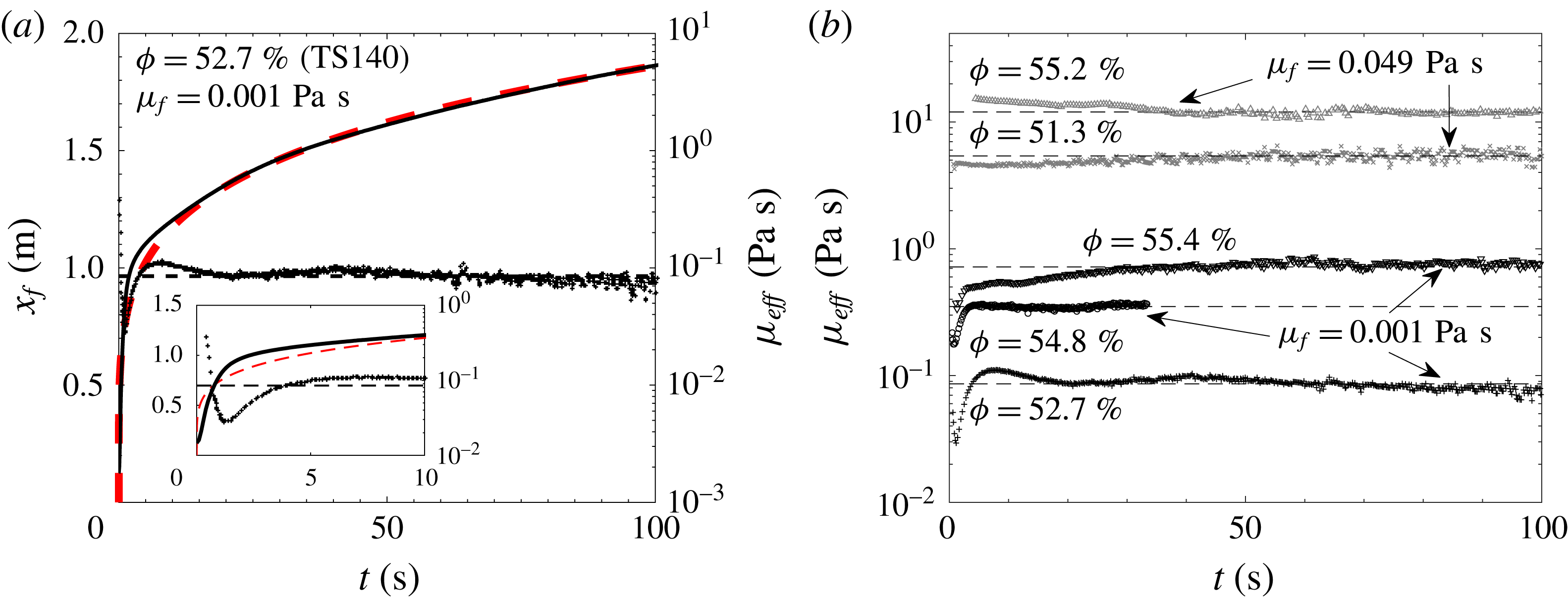
(a) The temporal evolution of the front
 $x_{f}$
and the effective viscosity
 $\unicode[STIX]{x1D707}_{eff}$
for a suspension composed of particles TS140 and
 $\unicode[STIX]{x1D707}_{f}=0.001~\text{Pa}~\text{s}$
at
 $\unicode[STIX]{x1D719}=52.7\,\%$
. The dashed line (red online) is the viscous asymptotic solution (4.1). The inset is a zoom at the early stages. (b) The temporal evolution of the effective viscosity
 $\unicode[STIX]{x1D707}_{eff}$
for various suspensions composed of particles TS140 and
 $\unicode[STIX]{x1D707}_{f}=0.001~\text{Pa}~\text{s}$
(black data) and
 $\unicode[STIX]{x1D707}_{f}=0.049~\text{Pa}~\text{s}$
(grey data).

The evolution of
 $\unicode[STIX]{x1D707}_{eff}$
obtained from (4.3) together with the corresponding front position
 $x_{f}$
is plotted as a function of time
 $t$
for
 $\unicode[STIX]{x1D707}_{f}=10^{-3}~\text{Pa}~\text{s}$
and
 $\unicode[STIX]{x1D719}=52.7\,\%$
(TS140) in figure 4(a). The viscous regime is reached when
 $\unicode[STIX]{x1D707}_{eff}$
becomes constant, i.e. for
 $t>20~\text{s}$
in this case. For
 $t<20~\text{s}$
, the quantity
 $\unicode[STIX]{x1D707}_{eff}$
is not an effective viscosity as it is not constant, and thus model (4.3) is not valid. However, the variation of this quantity gives some qualitative trends in the transient regime prior to the viscous regime. In particular, the front position evolves as
 $x_{f}\sim t^{\unicode[STIX]{x1D701}}$
with
 $\unicode[STIX]{x1D701}>0$
, and therefore
 $\text{d}X_{f}/\text{d}t\sim t^{5\unicode[STIX]{x1D701}-1}$
and
 $\unicode[STIX]{x1D707}_{eff}\sim t^{1-5\unicode[STIX]{x1D701}}$
from (4.3). It should be noted that from this simple scaling, the viscous regime corresponds to
 $\unicode[STIX]{x1D701}=1/5$
, i.e.
 $\unicode[STIX]{x1D707}_{eff}$
is constant. At the early stages,
 $\unicode[STIX]{x1D707}_{eff}$
is shown to decrease as a function of time (see the inset of figure 4
a), i.e.
 $\unicode[STIX]{x1D701}>1/5$
, in accordance with the acceleration and the inertial slumping regime. As
 $t$
increases,
 $\unicode[STIX]{x1D707}_{eff}$
is shown to suddenly increase, which implies
 $\unicode[STIX]{x1D701}<1/5$
. In particular, one obtains
 $\unicode[STIX]{x1D701}\sim 0.12$
, which corresponds to a front velocity decreasing faster than during the viscous regime. It should be noted that this regime is neither described by the different self-similar solutions nor reported in the literature. The height profile of the slumping current evolves from the inertial profile towards the viscous self-similar profile, inducing a strong deceleration of the front. This transient adaptation regime is also observed as an overshoot in the front position evolution in figure 5(a). This behaviour is also observed for
 $\unicode[STIX]{x1D719}=0$
(not shown here), and is therefore not linked to the presence of particles.
The evolution of
 $\unicode[STIX]{x1D707}_{eff}$
as a function of time for TS140 suspended particles and different values of
 $\unicode[STIX]{x1D707}_{f}$
and
 $\unicode[STIX]{x1D719}$
is shown in figure 4(b). Here, the black data and grey data correspond to
 $\unicode[STIX]{x1D707}_{f}=0.001~\text{Pa}~\text{s}$
and
 $\unicode[STIX]{x1D707}_{f}=0.049~\text{Pa}~\text{s}$
respectively. The trend of
 $\unicode[STIX]{x1D707}_{eff}$
is similar to the previous description for
 $\unicode[STIX]{x1D707}_{f}=0.001~\text{Pa}~\text{s}$
. For larger
 $\unicode[STIX]{x1D707}_{f}$
(
 $\unicode[STIX]{x1D707}_{f}=0.049~\text{Pa}~\text{s}$
here), the viscous regime is rapidly reached, leaving only a very brief, or even non-existent, inertial regime. The dashed lines in figure 4(b) show the obtained values of
 $\unicode[STIX]{x1D707}_{eff}$
when a plateau is reached. The obtained value
 $\unicode[STIX]{x1D707}_{eff}$
can then be used to support the model used to describe the front evolution as a function of time (4.1) (grey dashed line (red online) in figure 4
a).
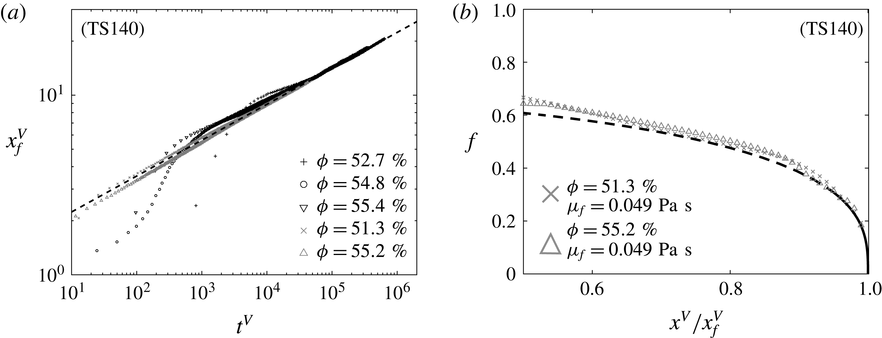
(a) The temporal evolution of the front position in viscous dimensionless form (4.4) for the same set of experiments as used in figure 4(b). (b) The shape function
 $f$
as a function of
 $(x^{V}/x_{f}^{V})$
for
 $\unicode[STIX]{x1D707}_{f}=0.049~\text{Pa}~\text{s}$
and
 $\unicode[STIX]{x1D719}=51.3\,\%$
(crosses) and
 $\unicode[STIX]{x1D719}=55.2\,\%$
(triangles). The dashed lines in (a) and (b) are the self-similar solutions
 $x_{f}^{(s)V}=\unicode[STIX]{x1D702}_{n}(t^{V})^{1/5}$
and
 $f(x/x_{f})=(3/10)^{1/3}(1-(x/x_{f})^{2})^{1/3}$
respectively.

Following relations (4.1) and (4.2), we can define the following viscous dimensionless variables:
 $$\begin{eqnarray}h^{V}=\frac{h}{H},\quad x^{V}=\frac{x}{L},\quad t^{V}=\frac{\unicode[STIX]{x1D70C}gH^{3}}{3\unicode[STIX]{x1D707}_{eff}L^{2}}t,\end{eqnarray}$$
to obtain the self-similar solution for the dimensionless front position and height profile
 $$\begin{eqnarray}\displaystyle x_{f}^{(s)V}=\unicode[STIX]{x1D702}_{n}(t^{V})^{1/5},\quad h^{(s)V}=\unicode[STIX]{x1D702}_{n}^{2/3}(t^{V})^{-1/5}f(x^{V}/x_{f}^{(s)V}). & & \displaystyle\end{eqnarray}$$
Figure 5(a) shows the dimensionless front position
 $x_{f}^{V}$
obtained from the experimental data as a function of the dimensionless time
 $t^{V}$
for the same set of experiments as used in figure 4(b). As
 $t^{V}$
increases, the suspension current evolves towards the apparent Newtonian viscous regime, for which the front position
 $x_{f}^{V}$
is nicely described by the asymptotic solution (4.5) represented by the dashed line in figure 5(a). Figure 5(b) shows the shape function
 $f$
as a function of
 $(x^{V}/x_{f}^{V})$
for
 $\unicode[STIX]{x1D707}_{f}=0.049~\text{Pa}~\text{s}$
and
 $\unicode[STIX]{x1D719}=51.3\,\%$
(crosses) and
 $\unicode[STIX]{x1D719}=55.2\,\%$
(triangles). The symbols correspond to experimental data for which the shape function is determined as
 $f=h^{V}x^{V}\unicode[STIX]{x1D702}_{n}^{-5/3}$
, while the dashed line corresponds to the self-similar solution. The depth profiles shown here are in excellent agreement with the self-similar profile (4.5) at least for
 $0.5\leqslant x^{V}/x_{f}^{V}\leqslant 1$
.
The relative viscosity
 $\unicode[STIX]{x1D707}_{eff}/\unicode[STIX]{x1D707}_{f}$
as a function of the volume fraction of particles
 $\unicode[STIX]{x1D719}$
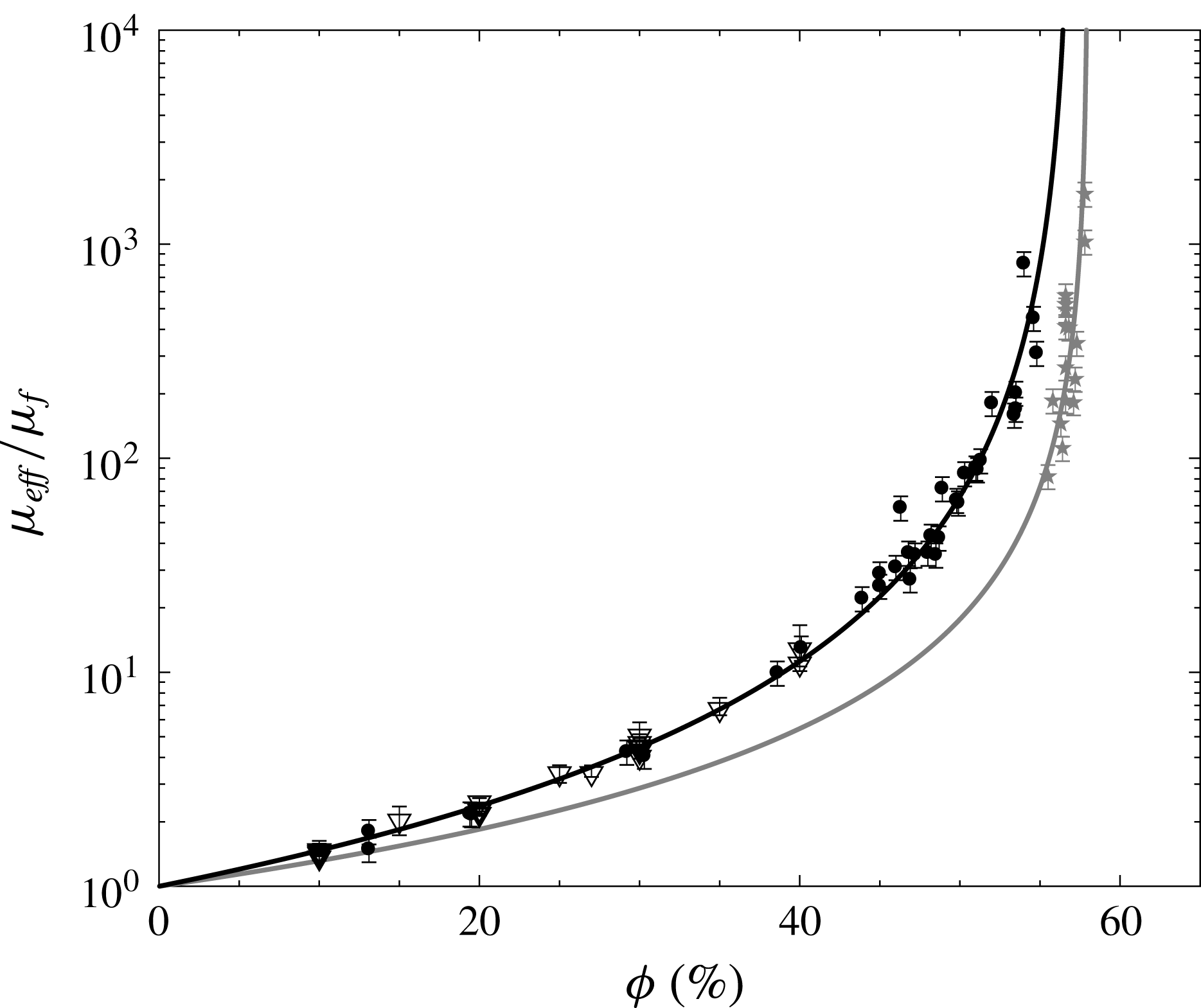
. The black circles and grey stars represent the relative viscosity of suspensions using protocols I and II respectively. For comparison, the triangles represent the relative viscosity of suspensions obtained using the serrated parallel-plate rheometer for protocol I. The solid lines represent the Krieger–Dougherty model (1.2) with
 $\unicode[STIX]{x1D719}_{m}=57.0\pm 1.0\,\%$
and
 $\unicode[STIX]{x1D6FC}\unicode[STIX]{x1D719}_{m}=2$
(black) and
 $\unicode[STIX]{x1D719}_{m}=58.0\pm 0.5\,\%$
and
 $\unicode[STIX]{x1D6FC}=2.5$
, i.e.
 $\unicode[STIX]{x1D6FC}\unicode[STIX]{x1D719}_{m}\sim 1.45\pm 0.01$
(grey).

From the previous analysis, it has been shown that the effective viscosity of the suspension can be determined from the dynamics of the front position (figure 4
a). It is thus possible to access the rheology of the suspension as a function of
 $\unicode[STIX]{x1D707}_{f}$
and
 $\unicode[STIX]{x1D719}$
for all suspensions used in the present study, as long as they enter an apparent Newtonian viscous regime. In figure 6, the relative viscosity
 $\unicode[STIX]{x1D707}_{eff}/\unicode[STIX]{x1D707}_{f}$
of the suspensions is plotted as a function of
 $\unicode[STIX]{x1D719}$
for all experiments. In this figure, dark (respectively grey) symbols correspond to experimental protocol I (respectively II). Uncertainties are shown with the error bars on these symbols, which are discussed in the Appendix. Empty symbols represent measurements performed with a Haake Mars III rheometer using a serrated parallel-plate geometry.
Only suspensions composed of particles TS40 and TS140 and prepared with protocol I have been used for rheometer measurements. In this case, the viscosity is obtained as the ratio of a measured shear stress to the shear rate imposed by the rheometer device. A ramp of increasing shear rate from
 $0.01~\text{s}^{-1}$
to
 $100~\text{s}^{-1}$
is covered, with a gap between the two serrated plates of
 $2~\text{mm}$
, i.e. large compared with the particle size. For a volume fraction
 $\unicode[STIX]{x1D719}\lesssim 35\,\%$
, the viscosity is well characterized. Above this volume fraction, the determination of the suspension rheology was more difficult and was not found to be reliable.
In figure 6, we can first notice that the effective viscosity increases with
 $\unicode[STIX]{x1D719}$
in all cases and is well fitted by a Krieger–Dougherty model (1.2) (see solid lines). For protocol I, the best approximation is found for
 $\unicode[STIX]{x1D6FC}\unicode[STIX]{x1D719}_{m}=2$
, in which case one obtains
 $\unicode[STIX]{x1D719}_{m}=57.0\pm 1.0\,\%$
(black line). For protocol II,
 $\unicode[STIX]{x1D6FC}=2.5$
is found to be a better exponent to fit the experimental data. In this case, one finds
 $\unicode[STIX]{x1D719}_{m}=58.0\pm 0.5\,\%$
(grey line). As observed in figure 6, all of the data are well defined by these two solutions, which correspond to the range of
 $\unicode[STIX]{x1D719}_{m}$
and
 $\unicode[STIX]{x1D6FC}$
found in the literature (see Ovarlez et al.
Reference Ovarlez, Bertrand and Rodts2006; Huang & Bonn Reference Huang and Bonn2007; Mueller et al.
Reference Mueller, Llewellin and Mader2010; Boyer et al.
Reference Boyer, Guazzelli and Pouliquen2011; Dbouk et al.
Reference Dbouk, Lobry and Lemaire2013; Mari et al.
Reference Mari, Seto, Morris and Denn2014, for instance), whatever the protocol used to make the suspension and the method used to extract the effective viscosity. Nevertheless, the set of data presented in figure 6 allows us to clearly distinguish the two protocols. In particular, the obtained effective viscosity is slightly larger for protocol I than for protocol II. This result clearly highlights the influence of the short-range interaction at the microscopic scale between the particles (Gallier et al.
Reference Gallier, Lemaire, Peters and Lobry2014; Mari et al.
Reference Mari, Seto, Morris and Denn2014). Here, the presence of air bubbles trapped at the surfaces of the particles in protocol I is probably the reason for a change in the short-range interaction, which leads to an increase in dissipation when the suspension is sheared.
5 Apparent non-Newtonian viscous regime
5.1 Shear-thinning versus shear-thickening
The previous section focused on the viscous regime considering that the suspension behaves as an idealized Newtonian fluid, for which the effective viscosity only varies with
 $\unicode[STIX]{x1D719}$
. It allowed us to extract the pertinent viscous scale, i.e. the effective viscosity, which controls the dynamics of the current in this regime. However, a slow evolution of
 $\unicode[STIX]{x1D707}_{eff}$
with time is often observed for dense suspensions, typically
 $\unicode[STIX]{x1D719}>35\,\%$
for protocol I and
 $\unicode[STIX]{x1D719}>55\,\%$
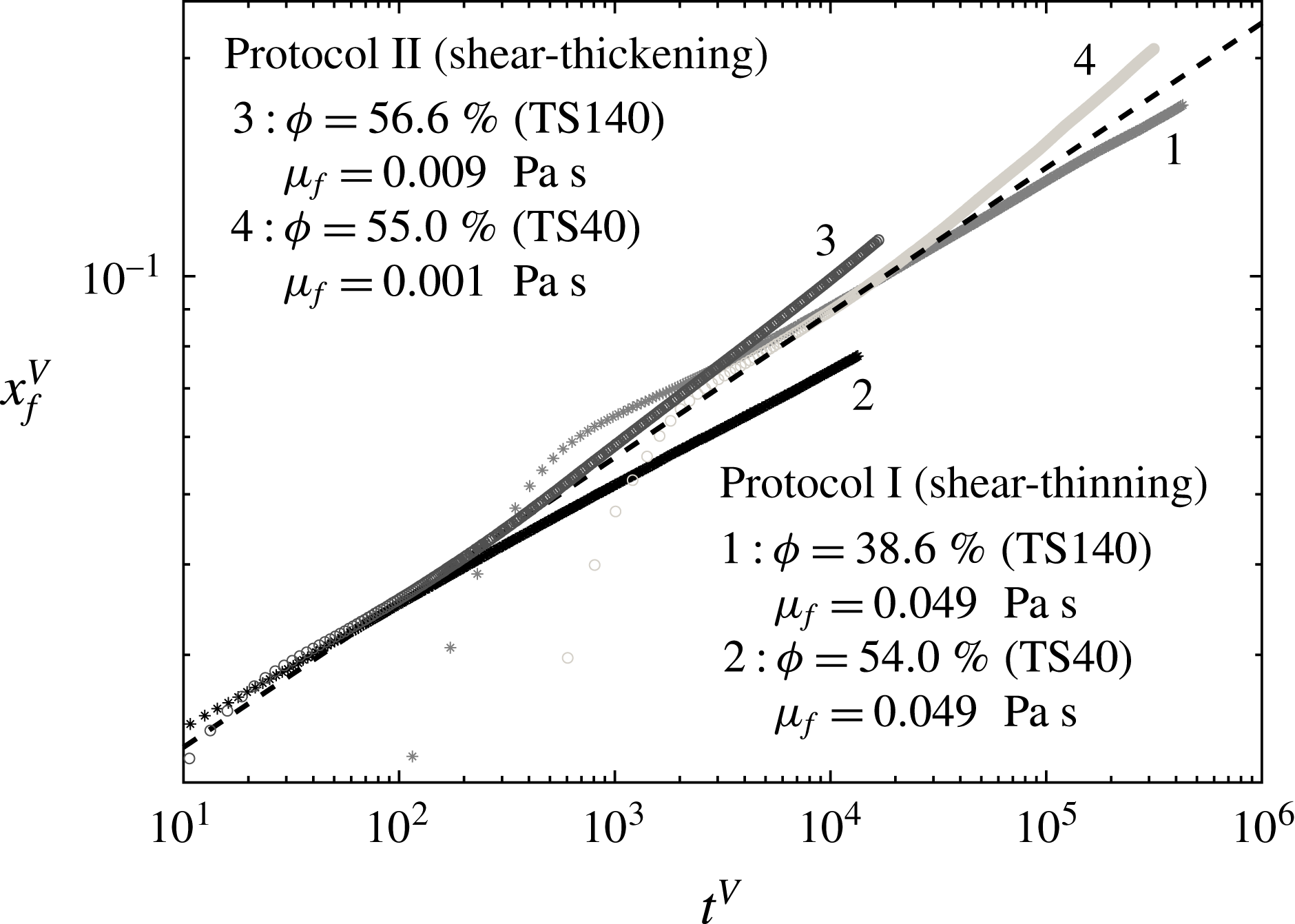
for protocol II, which appears as a deviation of the front evolution from the apparent Newtonian viscous solution (see figure 7). We can first notice that this deviation can be clearly distinguished for the two protocols. Even if the front position is shown to deviate from the Newtonian solution in both cases, the evolution associated with protocol I is observed to slow down, while it accelerates for protocol II. Moreover, the time scale on which the deviation occurs depends on
 $\unicode[STIX]{x1D719}$
for protocols I and II, but also on
 $d$
for protocol II. This evolution is here discussed in the light of shear-thinning and shear-thickening rheology, as often mentioned in the literature dealing with suspensions. In particular, we will show in the following that the two behaviours can be associated with shear-thinning (respectively shear-thickening) for protocol I (respectively protocol II) on a long time scale.

In order to characterize this apparent non-Newtonian behaviour, the more general power-law model is detailed here. In particular, the shear stress
 $\unicode[STIX]{x1D70F}$
is now expressed as a function of the shear rate
 $\dot{\unicode[STIX]{x1D6FE}}$
as
 $\unicode[STIX]{x1D70F}=K_{eff}\dot{\unicode[STIX]{x1D6FE}}^{m}$
, with
 $K_{eff}$
and
 $m$
the consistency and the index of the apparent fluid respectively. In the frame of lubrication theory, the self-similar solution for a Newtonian viscous model, shown in the previous section, can be extended to a power-law type fluid (Gratton et al.
Reference Gratton, Minotti and Mahajan1999; Piau & Debiane Reference Piau and Debiane2005; Di Federico et al.
Reference Di Federico, Malavasi and Cintoli2006), with the front position and height profile written as
 $$\begin{eqnarray}\displaystyle & \displaystyle x_{f}^{(s)}(t)=\unicode[STIX]{x1D702}_{n}\left[\frac{m}{2m+1}\left(\frac{\unicode[STIX]{x1D70C}g}{K_{eff}}\right)^{1/m}A^{(m+2)/m}t\right]^{m/(2m+3)}, & \displaystyle\end{eqnarray}$$
 $$\begin{eqnarray}\displaystyle & \displaystyle h^{(s)}(x,t)=\unicode[STIX]{x1D702}_{n}^{(1+m)/(2+m)}\left[\frac{2m+1}{m}\left(\frac{K_{eff}}{\unicode[STIX]{x1D70C}g}\right)^{1/m}\frac{A^{(m+1)/m}}{t}\right]^{m/(2m+3)}f(x/x_{f}), & \displaystyle\end{eqnarray}$$
where
 $\unicode[STIX]{x1D702}_{n}=[\int _{0}^{1}f(x/x_{f})\text{d}(x/x_{f})]^{-(2+m)/(3+2m)}$
is a constant that depends on
 $m$
and the shape function
 $f(x/x_{f})=[(m/(2m+3))^{m}((m+2)/(m+1))(1-(x/x_{f})^{m+1})]^{1/(m+2)}$
is obtained analytically. It should be noted that for
 $m=1$
, we recover the Newtonian solution (4.1)–(4.2).
Defining the following new dimensionless variables:
 $$\begin{eqnarray}h^{N}=\frac{h}{H},\quad x^{N}=\frac{x}{L},\quad t^{N}=\frac{m}{2m+1}\left(\frac{\unicode[STIX]{x1D70C}g}{K_{eff}}\right)^{1/m}\frac{H^{(m+2)/m}}{L^{(m+1)/m}}t,\end{eqnarray}$$
the self-similar solution for the dimensionless front position and height profile reads
 $$\begin{eqnarray}\displaystyle x_{f}^{(s)N}=\unicode[STIX]{x1D702}_{n}(t^{N})^{m/(2m+3)},\quad h^{(s)N}=\unicode[STIX]{x1D702}_{n}^{(1+m)/(2+m)}(t^{N})^{-m/(2m+3)}f(x^{N}/x_{f}^{(s)N}). & & \displaystyle\end{eqnarray}$$
In order to obtain
 $K_{eff}$
and
 $m$
from the front evolution in the experiments, a procedure similar to the one used to extract
 $\unicode[STIX]{x1D707}_{eff}$
in § 4 is used. Here,
 $X_{f}=(x_{f}/\unicode[STIX]{x1D702}_{n})^{(2m+3)/m}$
, and the derivative procedure explained previously, which now leads to
 $K_{eff}$
, therefore necessitates that we know
 $m$
. However, model (5.1) is valid only for constant
 $\text{d}X_{f}/\text{d}t$
. The value of
 $m$
is therefore found to satisfy this condition. The value of
 $K_{eff}$
is then obtained with the procedure used to evaluate
 $\unicode[STIX]{x1D707}_{eff}$
with the viscous Newtonian model in § 4. The evolution of the front position is shown in figure 8 for protocol I (figure 8
a) and protocol II (figure 8
b), with the appropriate scalings obtained from the obtained rheological parameters (see figure 9 discussed in the following). It can first be noted that this new rheological model allows the dimensionless front evolution to be collapsed on a longer time scale than that using the Newtonian model as in the previous section. We now discuss protocols I and II independently, as they highlight significant differences in the rheological parameters.
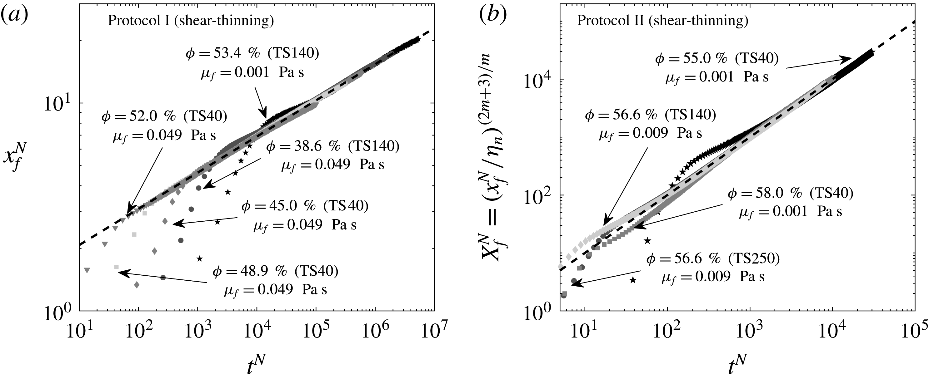
The evolution of the front position
 $x_{f}^{N}$
for protocol I (a) and the variable
 $X_{f}^{N}=(x_{f}^{N}/\unicode[STIX]{x1D702}_{n})^{(2m+3)/m}$
for protocol II (b) as a function of time
 $t^{N}$
in dimensionless form (5.3). The dashed lines (- - -) represent the self-similar solution (5.4) with
 $m=0.8$
(i.e.
 $x_{f}^{(s)N}\sim 1.39(t^{N})^{0.17}$
) (a) and
 $X_{f}^{N}=t^{N}$
(b).

For protocol I, figure 8(a) shows the evolution of the dimensionless front position
 $x_{f}^{N}$
as a function of the dimensionless time
 $t^{N}$
for
 $\unicode[STIX]{x1D719}=53.4\,\%$
(TS140) and
 $\unicode[STIX]{x1D707}_{f}=0.001~\text{Pa}~\text{s}$
(stars),
 $\unicode[STIX]{x1D719}=38.6\,\%$
(TS140) and
 $\unicode[STIX]{x1D707}_{f}=0.049~\text{Pa}~\text{s}$
(circles),
 $\unicode[STIX]{x1D719}=45.0\,\%$
(TS40) and
 $\unicode[STIX]{x1D707}_{f}=0.049~\text{Pa}~\text{s}$
(diamonds),
 $\unicode[STIX]{x1D719}=48.9\,\%$
(TS40) and
 $\unicode[STIX]{x1D707}_{f}=0.049~\text{Pa}~\text{s}$
(squares) and
 $\unicode[STIX]{x1D719}=52.0\,\%$
(TS40) and
 $\unicode[STIX]{x1D707}_{f}=0.049~\text{Pa}~\text{s}$
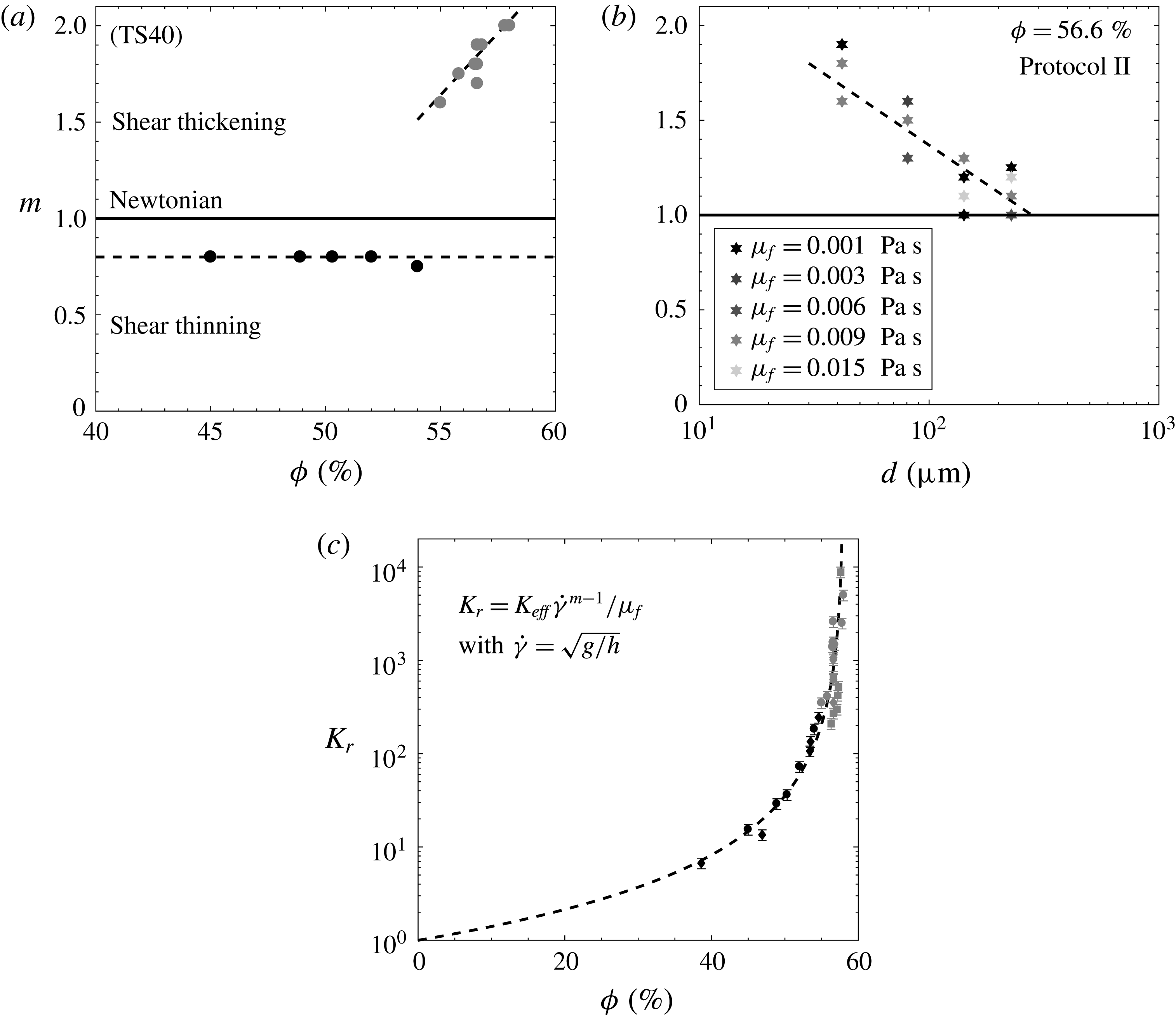
(triangles). The dashed line corresponds to the self-similar solution (5.4). It is shown to be in very good agreement with the experimental data. From these results, no clear trend is found for the index
 $m$
for particles TS40 (black symbols in figure 9
a) and other sizes (not shown here). The index of the suspension is therefore considered as constant,
 $m=0.8\pm 0.1$
, and suggests a shear-thinning behaviour, at least for
 $\unicode[STIX]{x1D719}>35\,\%$
, on a long time scale for protocol I. Moreover, the consistency
 $K_{eff}$
clearly increases with the volume fraction
 $\unicode[STIX]{x1D719}$
and is independent of the size of the particles and the interstitial fluid (figure 9
c). One can note that the dimensionless consistency
 $K_{r}=K_{eff}\dot{\unicode[STIX]{x1D6FE}}^{m-1}/\unicode[STIX]{x1D707}_{f}$
, with
 $\dot{\unicode[STIX]{x1D6FE}}=\sqrt{g/h}$
the shear rate, exhibits a trend that is similar to the one obtained for the relative viscosity
 $\unicode[STIX]{x1D707}_{eff}/\unicode[STIX]{x1D707}_{f}$
as a function of the volume fraction (see § 4). In particular, the evolution of
 $K_{r}$
with
 $\unicode[STIX]{x1D719}$
is surprisingly well fitted by a Krieger–Dougherty type model similar to (1.2). The obtained parameters are
 $\unicode[STIX]{x1D719}_{m}=58.0\pm 1.0\,\%$
and
 $\unicode[STIX]{x1D6FC}\unicode[STIX]{x1D719}_{m}=1.8\pm 0.1$
(red solid line in figure 9
c).
(a) The index
 $m$
as a function of the volume fraction
 $\unicode[STIX]{x1D719}$
for protocol I (black data) and protocol II (grey data). Only particles TS40 are considered here. (b) The index
 $m$
as a function of the diameter of particles
 $d$
for protocol II and
 $\unicode[STIX]{x1D719}=56.6\,\%$
. The viscosity of the interstitial fluid is between
 $0.001~\text{Pa}~\text{s}$
(black grey) and
 $0.015~\text{Pa}~\text{s}$
(light grey). (c) The normalized consistency
 $K_{r}$
as a function of the volume fraction
 $\unicode[STIX]{x1D719}$
for various viscosities of the interstitial fluid (i.e.
 $\unicode[STIX]{x1D707}_{f}=[0.001,0.049]~\text{Pa}~\text{s}$
) and particles TS40 (circles), TS140 (diamonds) and TS250 (squares). The dashed line is the Krieger–Dougherty model with
 $\unicode[STIX]{x1D719}_{m}=58.0\pm 1.0\,\%$
and
 $\unicode[STIX]{x1D6FC}\unicode[STIX]{x1D719}_{m}=1.8\pm 0.1$
.

The case of protocol II, where Triton X-100 was incorporated into the mixture, is shown in figure 8(b), where the evolution of
 $X_{f}^{N}=(x_{f}^{N}/\unicode[STIX]{x1D702}_{n})^{(2m+3)/m}$
is plotted as a function of
 $t^{N}$
for
 $\unicode[STIX]{x1D707}_{f}=[0.001,0.009]~\text{Pa}~\text{s}$
and various values of
 $\unicode[STIX]{x1D719}$
obtained from the experimental data (symbols) and the model (5.4) (dashed line). A very good agreement between experiments and the self-similar theory is observed. Here, the variation of
 $m$
is more pronounced and is found to lie in the interval
 $m\in [1.5,2]$
and to increase with
 $\unicode[STIX]{x1D719}$
for particles TS40 (grey circles in figure 9
a). It should be noted that
 $m=2$
would correspond to an inertial Bagnold regime for which the shear stress is a quadratic function of the shear rate. For the other sizes (not shown here), the variation of
 $m$
is in the interval
 $m\in [1,1.5]$
and no clear trends are observed with respect to
 $\unicode[STIX]{x1D719}$
. Only a shear-thickening behaviour is therefore observed for
 $\unicode[STIX]{x1D719}>55\,\%$
and protocol II. In this case, once the slumping suspension reaches the viscous regime, the velocity deviates slightly from the viscous scaling and the current progresses faster than expected for the effective viscosity of the suspension. Shear-thickening of the suspension flow is observed for all particle sizes and viscosities
 $\unicode[STIX]{x1D707}_{f}$
of the interstitial fluid but is more clearly quantified for TS40 and
 $\unicode[STIX]{x1D707}_{f}=10^{-3}~\text{Pa}~\text{s}$
. Figure 9(b) shows clearly the influence of the particle size
 $d$
on
 $m$
, which decreases with increasing diameter, unlike protocol I where
 $m$
is found to be constant. The shades of grey from dark (
 $\unicode[STIX]{x1D707}_{f}=0.001~\text{Pa}~\text{s}$
) to light (
 $\unicode[STIX]{x1D707}_{f}=0.015~\text{Pa}~\text{s}$
) grey do not show a significant influence of the interstitial fluid on
 $m$
compared with the influence of
 $d$
, at least in this range of parameters. Moreover, the normalized consistency
 $K_{r}$
is in good agreement with a Krieger–Dougherty type model with the same parameters (
 $\unicode[STIX]{x1D719}_{m}=58.0\pm 1.0\,\%$
and
 $\unicode[STIX]{x1D6FC}\unicode[STIX]{x1D719}_{m}=1.8\pm 0.1$
) obtained with a shear-thinning behaviour, i.e. with protocol I.
In this section, we have highlighted the most significant difference of the slumping dynamics for protocols I and II. This difference is only observed when the viscous dissipation controls the flow. Even if not explicitly proved here, the shear-thinning and shear-thickening behaviours observed here can be explained as follows. The short-range interactions in protocol I are probably controlled by air bubble interactions. Such interactions induce a more significant resistance at small shear rate while it breaks at high shear rate. This therefore explains the shear-thinning behaviour as observed in foam dynamics (Cohen-Addad, Hohler & Pitois Reference Cohen-Addad, Höhler and Pitois2013). On the other hand, in protocol II, such short-range interaction disappears. The observed shear-thickening trend is consistent with some observations on neutrally buoyant suspensions found in the literature (see Fall et al.
Reference Fall, Lemaitre, Bertrand, Bonn and Ovarlez2010, for instance). The shear-thickening behaviour observed here could be attributed to two processes, particle inertia and particle migration. First, it should be noted that when
 $\unicode[STIX]{x1D719}\rightarrow \unicode[STIX]{x1D719}_{m}$
, the obtained value of
 $m$
approaches
 $2$
at least for small enough particles TS40 (figure 9
a), which is in accordance with a Bagnold regime, dominated by the inertia of the particles, as observed by Fall et al. (Reference Fall, Lemaitre, Bertrand, Bonn and Ovarlez2010). The transition from the apparent Newtonian fluid to the apparent shear-thickening fluid could therefore be defined in terms of the Bagnold number. Using the definition presented in § 2.3, the transition is observed for
 $Ba\sim 10^{-1}$
, which actually lies in the large range obtained in the literature (Bagnold Reference Bagnold1954; Fall et al.
Reference Fall, Lemaitre, Bertrand, Bonn and Ovarlez2010; Trulsson et al.
Reference Trulsson, Andreotti and Claudin2012). Second, the decrease of
 $m$
with
 $d$
in the shear-thickening regime (figure 9
b) could be a signature of particle migration, which strongly depends on the particle size. In such a scenario, particle migration, which would separate particles from the bottom wall, leads to a strong heterogeneity of
 $\unicode[STIX]{x1D719}$
in the suspension and the possible emergence of a thin layer close to the bottom plane which lubricates the suspension current.
However, suitable local measurements are needed to confirm this scenario. This question is therefore postponed to a future work. To finish with, when the exponent
 $m$
is selected, the dimensionless consistency
 $K_{r}$
is found to collapse onto a single
 $\unicode[STIX]{x1D719}$
curve for all of the experiments performed in the present study, including all protocols,
 $\unicode[STIX]{x1D719}$
,
 $\unicode[STIX]{x1D707}_{f}$
and
 $d$
.
5.2 Viscoplastic behaviour
In the previous sections, a singularity of the effective viscosity, or consistency, has been observed at
 $\unicode[STIX]{x1D719}=\unicode[STIX]{x1D719}_{m}$
. Even if the specific value of
 $\unicode[STIX]{x1D719}_{m}$
depends on the protocol, it is below the maximum packing that can be obtained for a granular material. Experiments can therefore be performed above
 $\unicode[STIX]{x1D719}_{m}$
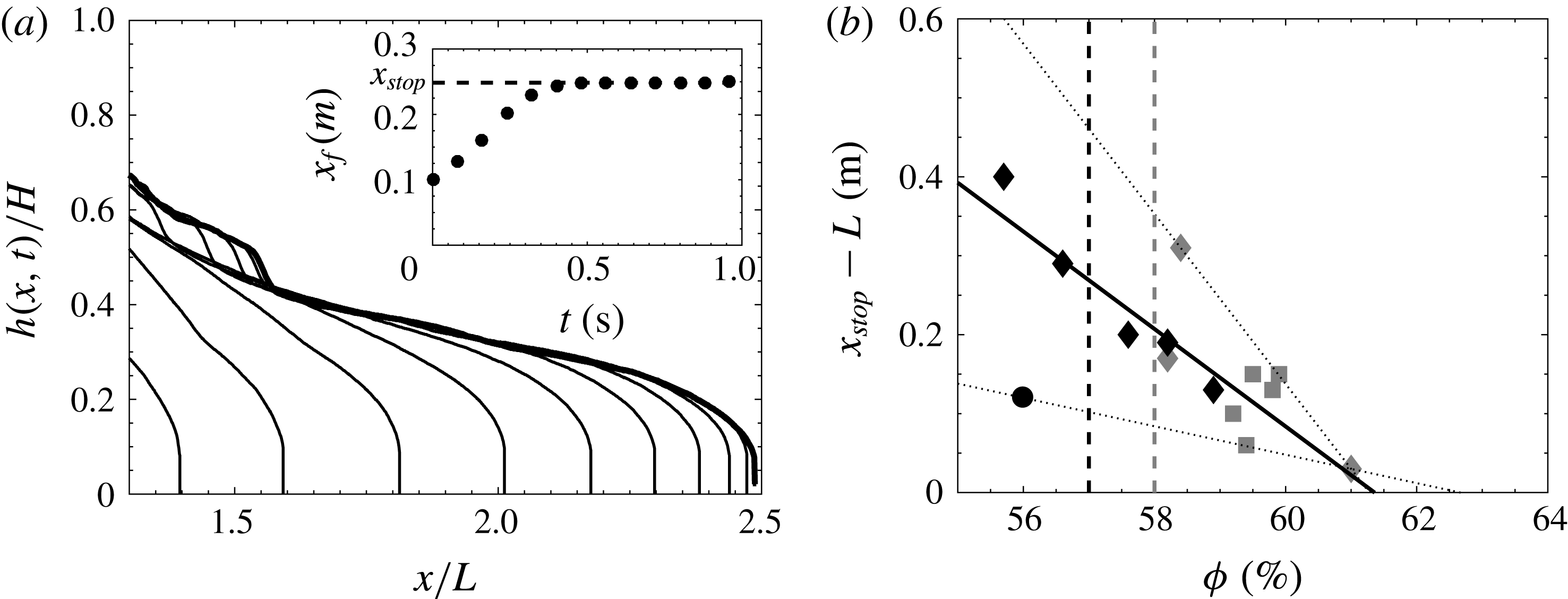
. Figure 10 shows the height profile as a function of time for a volume fraction
 $\unicode[STIX]{x1D719}=59.9$
% (with
 $\unicode[STIX]{x1D707}_{f}=0.001~\text{Pa}~\text{s}$
, particle size TS250 and protocol II). The time evolution of the front position
 $x_{f}$
is shown in the inset of figure 10. It can be noted that the front reaches a plateau at a finite time, i.e. the current stops, after a short viscous phase. It should be noted that this behaviour is obtained whatever the particle size (TS40, TS140 and TS250), interstitial fluid viscosity (
 $\unicode[STIX]{x1D707}_{f}=0.001~\text{Pa}~\text{s}$
and
 $\unicode[STIX]{x1D707}_{f}=0.049~\text{Pa}~\text{s}$
) and protocol (protocol I and protocol II).
(a) The temporal evolution of the height profile for a suspension current for
 $\unicode[STIX]{x1D719}=59.9\,\%$
(TS250,
 $\unicode[STIX]{x1D707}_{f}=0.001~\text{Pa}~\text{s}$
, protocol II). The profiles correspond to time
 $t=0.12{-}0.76~\text{s}$
in steps of
 $0.04~\text{s}$
. The inset represents the front position
 $x_{f}$
as a function of time. The dashed line is the runout length
 $x_{stop}$
of the viscoplastic suspension. (b) The evolution of the spreading length
 $(x_{stop}-L)$
as a function of the volume fraction
 $\unicode[STIX]{x1D719}$
for protocol I (black) and protocol II (grey) and particles TS40 (circles), TS140 (diamonds) and TS250 (squares). The dashed lines are
 $\unicode[STIX]{x1D719}_{m}=57\,\%$
and
 $\unicode[STIX]{x1D719}_{m}=58\,\%$
, used in the Krieger–Dougherty model in § 4 for protocols I and II respectively. The solid line is the best fit,
 $x_{stop}-L=-0.0617\unicode[STIX]{x1D719}+3.787$
, and the two dotted lines are the extreme fits.

As in the case of a granular collapse, a maximum spreading length can therefore be extracted in this case. In the granular case, the initial aspect ratio of the column has been shown to be the parameter that mostly influences the spreading length. In the present case, we are interested in the impact of the volume fraction
 $\unicode[STIX]{x1D719}$
. Figure 10(b) shows the evolution of the spreading length
 $(x_{stop}-L)$
as a function of
 $\unicode[STIX]{x1D719}$
for protocol I (dark symbols) and protocol II (grey symbols). It should be noted that for protocol I, viscoplastic behaviours are observed for
 $\unicode[STIX]{x1D719}<\unicode[STIX]{x1D719}_{m}$
(dashed vertical black line), in accordance with the shear-thinning behaviour highlighted in the previous section with this protocol. For protocol II, the flow only stops when
 $\unicode[STIX]{x1D719}>\unicode[STIX]{x1D719}_{m}$
(dashed vertical grey line). In any case,
 $(x_{stop}-L)$
is shown to decrease with
 $\unicode[STIX]{x1D719}$
with a roughly linear trend (solid line in figure 10
b). An extrapolation of this linear trend at
 $x_{stop}-L=0$
, i.e. the initial column remains undeformed, allows us to extract a volume fraction
 $\unicode[STIX]{x1D719}_{M}$
in the range
 $[0.609,0.627]$
above which no flow can occur, i.e. the initial column remains static. It can be noted that
 $\unicode[STIX]{x1D719}_{M}$
is close to the maximum packing fraction. This observation is discussed in the following in terms of an apparent plasticity of the suspension, even if a viscoplastic regime would remain striking in this experiment for two reasons. First, no homogeneous flow is expected to occur above the maximum volume fraction
 $\unicode[STIX]{x1D719}_{m}$
(Fall et al.
Reference Fall, Bertrand, Ovarlez and Bonn2009; Boyer et al.
Reference Boyer, Guazzelli and Pouliquen2011; Trulsson et al.
Reference Trulsson, Andreotti and Claudin2012). Second, only a normal stress in the granular phase can lead to a Coulomb type yield stress in this system.
In the case of a neutrally buoyant suspension, the granular pressure is expected to vanish, and therefore no yield stress should be observed, unlike the case of turbidity currents (Hallworth & Huppert Reference Hallworth and Huppert1998). However, due to the very high constraint imposed by the initial sharp geometry, the volume fraction
 $\unicode[STIX]{x1D719}_{m}$
, which is close to a loose volume fraction, is probably not sufficient to maintain the column. In this case, the suspension can locally expand to allow a local flow close to the sharp interface. This local expansion imposes a restoring force acting on the granular phase to conserve the initial volume, described as the surface tension by Fall et al. (Reference Fall, Bertrand, Ovarlez and Bonn2009) and Andreini et al. (Reference Andreini, Ancey and Epely-Chauvin2013). This force then plays the role of the normal stress which then leads to a yield stress in the granular material. The order of this surface tension imposed pressure can be estimated as
 $2\unicode[STIX]{x1D70E}/d$
(Fall et al.
Reference Fall, Bertrand, Ovarlez and Bonn2009; Andreini et al.
Reference Andreini, Ancey and Epely-Chauvin2013), where
 $\unicode[STIX]{x1D70E}$
is the interfacial tension. For a suspension composed of particles of diameter
 $d=40~\unicode[STIX]{x03BC}\text{m}$
or
 $d=250~\unicode[STIX]{x03BC}\text{m}$
in water, the order is found to be
 $500$
–
 $3000~\text{Pa}$
close to the hydrostatic pressure
 $\unicode[STIX]{x1D70C}gH\sim 1000$
Pa, which is the initial driving force. The suspension can thus highlight an apparent viscoplastic behaviour up to a volume fraction
 $\unicode[STIX]{x1D719}_{M}$
, above which the packing allows the initial sharp interface to be maintained. Andreini et al. (Reference Andreini, Ancey and Epely-Chauvin2013) observed a similar trend, explained as a stick–slip of the suspension on the bottom wall due to a balance between the hydrostatic pressure and the capillarity pressure. In this case, the sudden stop of the suspension flow is also attributed to surface tension. It should be noted that stick–slip is observed here, but on a time scale that is very long, around
 $20$
minutes, compared with the collapse time scale
 ${\sim}1~\text{s}$
. We thus disregard the stick–slip phase and attribute this observation to an apparent plasticity of the suspension even if the mechanism is probably similar. Nevertheless, this scenario deserves a dedicated experimental study to quantify more precisely the influence of surface tension on the suspension and justify it as the only mechanism at the origin of these observations. It should be noted, for instance, that a stick–slip behaviour similar to the one described here has also been observed in another system without a free surface (Kulkarni, Metzger & Morris Reference Kulkarni, Metzger and Morris2010).
6 Conclusion
The collapse of non-colloidal and neutrally buoyant particles suspended in a Newtonian fluid column has been investigated. The dynamics of the current was characterized by varying the initial volume fraction of the suspension
 $\unicode[STIX]{x1D719}$
, the viscosity of the interstitial fluid
 $\unicode[STIX]{x1D707}_{f}$
, the diameter of the particles
 $d$
and the mixing protocol, i.e. the initial preparation of the suspension. The temporal evolution of the slumping highlighted two main regimes: (i) an inertial-dominated regime followed by (ii) a viscous-dominated regime, which can be described by shallow layer/lubrication models.
The inertial regime was only found for sufficiently high Reynolds number (typically
 $Re\gtrsim 1$
), based on the effective viscosity
 $\unicode[STIX]{x1D707}_{eff}$
of the suspension. This regime is characterized by a constant-speed slumping which is shown to scale as in the case of a classical inertial dam-break. In particular, the inertial slumping regime shows that the dimensionless front velocity scales as
 $\text{d}x_{f}^{I}/\text{d}t^{I}\sim 1.5\sqrt{gH}$
. Moreover, analysis of the transition time from this inertial slumping regime to the following viscous regime allows one to extract a first estimation of an effective viscosity
 $\unicode[STIX]{x1D707}_{eff}$
of the suspension as a function of
 $\unicode[STIX]{x1D719}$
as
 $\unicode[STIX]{x1D707}_{eff}\sim \unicode[STIX]{x1D6FD}(1-\unicode[STIX]{x1D719}/\unicode[STIX]{x1D719}_{m})^{-\unicode[STIX]{x1D6FC}\unicode[STIX]{x1D719}_{m}}$
, with
 $\unicode[STIX]{x1D719}_{m}\sim 76\,\%$
,
 $\unicode[STIX]{x1D6FC}\sim 5.3$
and
 $\unicode[STIX]{x1D6FD}\sim 0.96\times 10^{-3}~\text{Pa}~\text{s}$
, i.e. close to the Krieger–Dougherty model (1.2).
The viscous-dominated regime is observed as a decreasing-speed phase of the front evolution. This regime is more complex and highlights behaviour depending on the suspension parameters mentioned above. Lubrication models allow one to identify most of the situations when both Newtonian fluid and generalized power-law fluid – where the shear stress
 $\unicode[STIX]{x1D70F}$
is written as a function of the shear rate
 $\dot{\unicode[STIX]{x1D6FE}}$
such as
 $\unicode[STIX]{x1D70F}=\unicode[STIX]{x1D707}_{eff}\dot{\unicode[STIX]{x1D6FE}}$
and
 $\unicode[STIX]{x1D70F}=K_{eff}\dot{\unicode[STIX]{x1D6FE}}^{m}$
respectively – are considered. This macroscopic description of the slumping flow allows one to describe the unsteady dynamics of the suspension flow as apparent Newtonian and apparent non-Newtonian fluids regardless of the smaller-scale dynamics of the particles. The temporal evolution of the propagating front was then used to extract the rheological parameters of the fluid models.
First, an apparent Newtonian fluid is shown to be pertinent to describe the dynamics of the front at the early stages of the viscous-dominated regime. The obtained values of the effective viscosity
 $\unicode[STIX]{x1D707}_{eff}$
are shown to be in good agreement with measurements performed with a serrated parallel-plate rheometer as well as the Krieger–Dougherty model, i.e.
 $\unicode[STIX]{x1D707}_{eff}/\unicode[STIX]{x1D707}_{f}\sim (1-\unicode[STIX]{x1D719}/\unicode[STIX]{x1D719}_{m})^{-\unicode[STIX]{x1D6FC}\unicode[STIX]{x1D719}_{m}}$
. However, the parameters involved in the viscosity models seem to depend on the mixing protocol and two cases were distinguished: (i) protocol I for which
 $\unicode[STIX]{x1D719}_{m}\sim 57.0\pm 1.0\,\%$
,
 $\unicode[STIX]{x1D6FC}\unicode[STIX]{x1D719}_{m}=2$
and (ii) protocol II with
 $\unicode[STIX]{x1D719}_{m}\sim 58.0\pm 0.5\,\%$
,
 $\unicode[STIX]{x1D6FC}\unicode[STIX]{x1D719}_{m}=1.45\pm 0.01$
(i.e.
 $\unicode[STIX]{x1D6FC}=2.5$
). This observed difference was attributed to the local microscale interaction between particles which can strongly differ between the two protocols.
On a longer time scale that depends on
 $\unicode[STIX]{x1D719}$
, the front evolution is shown to slightly deviate from the apparent Newtonian model. In this case, the power-law model, indicating both shear-thinning (
 $m<1$
) and shear-thickening (
 $m>1$
) behaviours, is shown to be more appropriate to describe the front evolution. The present experiments indicate that the mixing protocol plays a crucial role in the selection of a shear-thinning or shear-thickening type of collapse, while the particle diameter
 $d$
and volume fraction
 $\unicode[STIX]{x1D719}$
play a significant role in
 $m$
only in the shear-thickening case, and
 $m$
is found in the interval
 $m\in [1,2]$
. More surprisingly, once the exponent
 $m$
is selected, it is found that the consistency parameter
 $K_{eff}\dot{\unicode[STIX]{x1D6FE}}^{(m-1)}/\unicode[STIX]{x1D707}_{f}$
, with
 $\dot{\unicode[STIX]{x1D6FE}}=\sqrt{g/h}$
the shear rate and
 $h$
the typical height of the current, only depends on
 $\unicode[STIX]{x1D719}$
and on neither the mixing protocol nor
 $d$
.
Finally, an apparent viscoplastic regime, characterized by a finite length spreading reached at finite time, is observed at high
 $\unicode[STIX]{x1D719}$
. This regime is mostly observed for volume fractions between
 $\unicode[STIX]{x1D719}_{m}$
and
 $\unicode[STIX]{x1D719}_{M}\in [0.609,0.627]$
close to the random close packing fraction. The appearance of an apparent yield stress in this experiment has been explained as a local granular expansion which induces a surface tension pressure, leading to a Coulomb type yield stress in the suspension. Above
 $\unicode[STIX]{x1D719}_{M}$
, the initial sharp interface can be maintained by the granular packing on opening the gate.
Acknowledgements
We are grateful to the Agence Française pour la Biodiversité which has supported this work. We thank M. J. Mercier and D. Anne-Archard for their help in the experimental protocol. Moreover, we thank the reviewers for their constructive remarks which helped to significantly improve this paper, in particular for having drawn our attention to the scaling
 $\unicode[STIX]{x1D70F}_{t}^{f}\sim \unicode[STIX]{x1D707}_{f}^{-1/4}$
.
Supplementary movies
Supplementary movies are available at https://doi.org/10.1017/jfm.2017.471.
Appendix. Uncertainties in the effective viscosity measurement
The viscosity measured here suffers from uncertainties due to a possible sidewall effect, model assumptions, temperature variation, etc. In order to quantify their influences on our results, we compared the viscosity obtained with a classical rheometer and our experimental model in the case of a single-phase fluid, i.e.
 $\unicode[STIX]{x1D719}=0$
, for which rheometer measurements are known to be robust. The results are shown in figure 11. We plot here
 $\unicode[STIX]{x1D707}_{R}$
(viscosity obtained with the rheometer) as a function of
 $\unicode[STIX]{x1D707}_{M}$
(found from the slumping model). The solid line shows
 $\unicode[STIX]{x1D707}_{M}=\unicode[STIX]{x1D707}_{R}$
. We actually find an offset which can be fitted as
 $\unicode[STIX]{x1D707}_{M}=1.3\unicode[STIX]{x1D707}_{R}$
(dashed line), corresponding to an overestimation of
 $30\,\%$
on the viscosity.
Viscosity measurements from the slumping model as a function of the viscosity obtained from rheometer measurements in the case of a viscous single-phase fluid.

It is worth noticing that in the range of parameters, time scales and length scales considered here, a time-independent viscosity (even if overestimated) was found from the model and allowed us to capture the time evolution of the front position during the entire viscous regime (see figure 4). This means that the influence of the undesired effects does not significantly evolve throughout an experimental run, and it is thus reasonable to assume that the possible time variation of such effects is negligible here.
In addition, as the suspension fluid highlights a similar dynamics to a viscous fluid in most of the runs, except when non-Newtonian behaviours show up, the influence of possible undesired effects on the viscosity is assumed to be similar for single fluids and suspensions. A key point here is the fact that the overestimation of the viscosity observed in figure 11 is roughly constant (systematically
 $30$
% larger than the ‘true’ viscosity) and independent of
 $\unicode[STIX]{x1D707}$
in the range of parameters considered here. This is the reason why we refer to this overestimation as a bias on the experimental results rather than an error. Thus, assuming that the possible influence of the walls (or other undesired effects) here leads to a bias on the obtained viscosity, the ratio
 $\unicode[STIX]{x1D707}_{eff}/\unicode[STIX]{x1D707}_{f}$
(figure 6), which is nothing but the ratio of viscosity for a given
 $\unicode[STIX]{x1D719}$
to the viscosity for
 $\unicode[STIX]{x1D719}=0$
(both obtained using the same procedure), should therefore remove this bias.
Nevertheless, in order to illustrate the possible influence of these undesired effects on the obtained quantitative results, we also report this bias as an error on the obtained viscosity by adding error bars around the mean value of the extracted viscosity in figures 6 and 9(c). In the latter, the errors were considered to be similar to those for a Newtonian viscous single-phase fluid. These error bars then probably overestimate the undesired effects. They are shown to be as small as the dispersion results (see figure 6 for instance) and therefore do not significantly affect the fitting parameters of the rheological models obtained for the large range of parameters considered here. It should be noted that the influence of these uncertainties has also been accounted for in the parameters of the obtained rheological models.