


1. Introduction
This article is devoted to solving a two-dimensional (2D)
 $\textbf{H}(\text{curl})$
-elliptic interface problem originating from Maxwell equations on unfitted meshes. Let
 $\Omega\subseteq\mathbb{R}^2$
be a bounded domain, and let it contain two subdomains
 $\Omega^{\pm}$
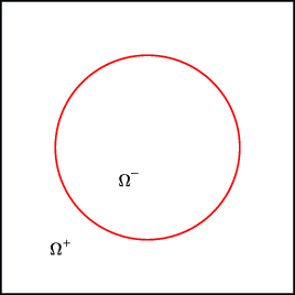
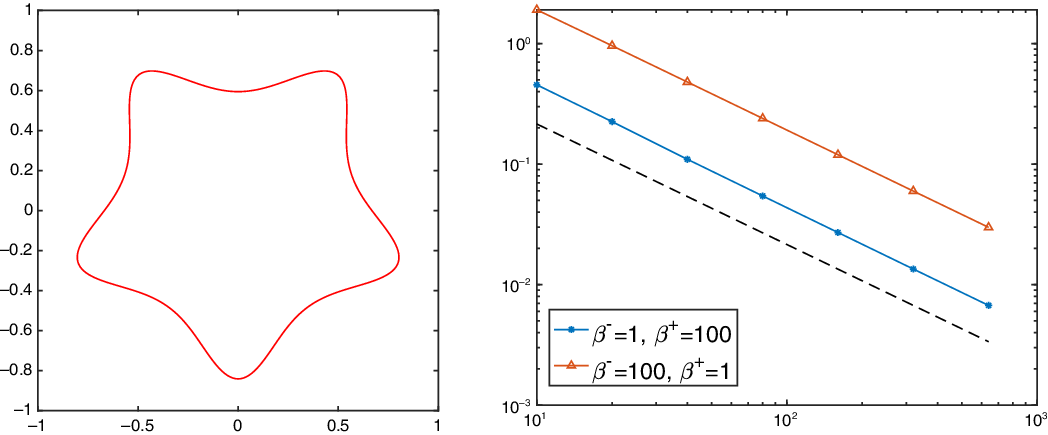
occupied by media with different electromagnetic properties. These two subdomains are partitioned by a curve (interface) which is assumed to be a smooth simple Jordan curve and does not touch the boundary as shown in Figure 1. The considered
 $\textbf{H}(\text{curl})$
-elliptic interface problem for an electric field
 $\textbf{u}\,:\,\Omega\rightarrow\mathbb{R}^2$
is given by
 \begin{align}\underline{ \text{curl}}\,\mu^{-1} \text{curl}\,\textbf{u} + \beta \textbf{u} = \textbf{f} \;\;\;\; & \text{in} \; \Omega = \Omega^- \cup \Omega^+,\end{align}
with
 $\textbf{f}\in\textbf{H}(\text{div};\,\Omega)$
, subject to the Dirichlet boundary condition:
 $\textbf{u}\cdot\textbf{t} = 0$
on
 $\partial\Omega$
, where the operator curl is for vector functions
 $\textbf{v}=[v_1,v_2]^t$
such that
 $\text{curl}\,\textbf{u}=\partial_{x_1}v_2 - \partial_{x_2}v_1$
while
 $\underline{\text{curl}}$
is for scalar functions v such that
 $\underline{\text{curl}}\,v = \left[ \partial_{x_2}v, - \partial_{x_1}v \right]^t$
with “t” denoting the transpose. We consider the following jump conditions at the interface:
 \begin{align}[\textbf{u}\cdot\textbf{t}]_{\Gamma} &\,:\!=\, \textbf{u}^+\cdot\textbf{t} - \textbf{u}^-\cdot\textbf{t} = 0, \end{align}
 \begin{align}[\mu^{-1}\text{curl}\,\textbf{u}]_{\Gamma} &\,:\!=\, \frac{1}{\mu^+}\text{curl}(\textbf{u}^+) - \frac{1}{\mu^-}\text{curl}(\textbf{u}^-) = 0, \end{align}
 \begin{align}[\beta\textbf{u}\cdot\textbf{n}]_{\Gamma} &\,:\!=\, \beta^+\textbf{u}^+\cdot\textbf{n} - \beta^-\textbf{u}^-\cdot\textbf{n} = 0,\end{align}
where
 $\textbf{n}$
and
 $\textbf{t}$
denote the normal and tangential vectors to
 $\Gamma$
, respectively, and
 $\mu=\mu^{\pm}$
and
 $\beta=\beta^{\pm}$
in
 $\Omega^{\pm}$
are assumed to be positive piecewise constant functions. The interface model (1.1) arises from each time step in a stable time-marching scheme for the eddy current computation [Reference Ammari, Buffa and Nédélec4, Reference Beck, Hiptmair, Hoppe and Wohlmuth13, Reference Dirks27], which serves as a magneto-quasistatic approximation by dropping the displacement current. It has been frequently used in low frequency and high-conductivity applications. In this model,
 $\mu$
denotes the magnetic permeability and
 $\beta\sim \sigma/\triangle t$
is scaling of the conductivity
 $\sigma$
by the time-marching step size
 $\triangle t$
. Note that the usual variational weak formulation of (1.1) can naturally take care of the jump conditions in (1.1b) and (1.1c), whereas (1.1d) comes from the underlying eddy current model [Reference Monk60]. We shall see that all the jump conditions in (1.1b)–(1.1d) will be used in the construction of the IFE functions. For simplicity, we only consider the homogeneous jump condition, and the non-homogeneous case can be handled by introducing an enriched function, see [Reference Gong, Li and Li31, Reference He, Lin and Lin38] and a recent work on theoretical analysis [Reference Adjerid, Babuška, Guo and Lin1].
The model domain.

Interface problems widely appear in a large variety of science and engineering applications. The interface problems related to Maxwell equations are of particular importance due to the omnipresent situation of electromagnetic fields propagating through multiple materials/media, such as simulation of magnetic actuators or design of nano/micro electric devices. In particular, we refer readers to the simulation of plasma [Reference Lu, Yang, Bai, Cao and He59] in electromagnetic fields and non-destructive testing techniques such as electromagnetic induction sensors [Reference Ammari, Chen, Chen, Volkov and Wang5] detecting buried low-metallic content.
Traditional finite element methods (FEMs) can be applied to solve interface problems based on interface-fitted meshes [Reference Babuška and Osborn12, Reference Li, Melenk, Wohlmuth and Zou52]. Particularly, many numerical methods have been developed to solve Maxwell interface problems on fitted meshes. In [Reference Hiptmair, Li and Zou41], the authors analysed a standard FEM and established an
 $\textbf{H}^1(\text{curl};\,\Omega)$
-extension theorem which is a very useful theoretical tool. In [Reference Huang and Zou49], the authors explicitly specified the dependence of error bounds on material parameters. The study on preconditioners can be found in [Reference Xu and Zhu65]. In addition, due to the potentially low regularity, there are many works focusing on adaptive FEMs, see [Reference Cai and Cao18, Reference Chen, Xiao and Zhang23, Reference Duan, Qiu, Tan and Zheng29] and the reference therein. However, it is time-consuming to generate fitted meshes in some applications, especially for complex interface geometry.
Alternatively, lots of research interests have been focussed on developing numerical methods with less interface-fitted mesh requirements. One approach is to locally generate a fitted mesh to the interface by further partitioning interface elements of a background unfitted mesh. But this approach requires the refined triangularisation to satisfy a maximal angle condition [Reference Babuška and Aziz9], which needs some extra effort, especially in 3D. Moreover, the resulting linear system could be more ill-conditioned since elements may largely shrink. In contrast, designing special FEMs for unfitted meshes has gained more and more attention. For instance, penalty-type methods [Reference Burman, Claus, Hansbo, Larson and Massing17, Reference Huang, Wu and Xiao50] employ two separate finite element (FE) spaces discontinuous across the interface and enforce the jump conditions by Nitsche’s penalties on the interface. Generalised FEMs [Reference Babuška and Osborn11] and multiscale FEMs [Reference Chu, Graham and Hou24, Reference Hou, Wu and Zhang45] construct some special non-polynomial shape functions on interface elements by solving local problems.
Immersed FEMs (IFE methods) fall into the direction of constructing special shape functions. Specifically, it constructs piecewise polynomials weakly satisfying jump conditions on interface elements [Reference Guo and Lin35, Reference Li54, Reference Lin, Lin and Zhang55]. In the past decades, IFE methods have been widely applied to different interface problems, including elasticity [Reference Guo, Lin and Lin36, Reference Lin, Sheen and Zhang57], fluid dynamics [Reference Adjerid, Chaabane and Lin2, Reference Wang, Zhang and Zhuang63] and so on. As a distinguishing feature of the IFE method, there is certain isomorphism between the immersed finite element (IFE) and FE spaces such that the size and structure of stiffness and mass matrices depend purely on the mesh. Existing works [Reference Guo33, Reference He, Lin, Lin and Zhang39, Reference Lin, Lin and Zhang56] show that it is particularly advantageous for moving interface problems. Our analysis reveals that the isomorphism with its stability is also the key to circumventing the ill-conditioning issue resulting from the shrinking subelements cut by the interface.
Despite their wide successful applications to various interface problems including fluid, elasticity and wave propagation, e.g., [Reference Becker, Burman and Hansbo14, Reference Groß and Reusken32, Reference Guo, Lin, Lin and Zhuang37], the aforementioned unfitted mesh methods are rarely applied to
 $\textbf{H}(\text{curl})$
-elliptic interface problems. In fact, the
 $\textbf{H}(\text{curl})$
interface problem is significantly distinguished from its
 $H^1$
counterpart due to the different underlying Sobolev space
 $\textbf{H}^1(\text{curl};\,\Omega)$
that has much lower regularity than
 $H^{2}(\Omega)$
. For the
 $\textbf{H}(\text{curl})$
case, the expected optimal convergence of FEM computation highly relies on the conformity of approximation spaces. Particularly, non-conforming methods demand estimates on element boundary, but there only holds
 \begin{equation}h^{-1/2}_K \| \textbf{u} - \pi_e \textbf{u} \|_{L^2(e)} \lesssim \| \textbf{u} \|_{\textbf{H}^1(\text{curl};\,K)},\end{equation}
where
 $\pi_e$
is a projection to some polynomial space on one edge e of an element K, see Lemma 5.52 in [Reference Monk60]. Namely,
 $\text{curl}\textbf{u}\in H^1(K)$
does not really help in enhancing the regularity and improving the convergence order, which is the essential difference from the
 $H^1$
case. Thus, even for the regularity assumption
 $\textbf{H}^1(\text{curl};\,\Omega)$
, the estimate in (1.2) indicates no convergence at all, which challenges many non-conforming methods. The issue even causes troubles for the analysis of standard discontinuous Galerkin (DG) methods on fitted meshes [Reference Houston, Perugia, Schneebeli and Schötzau46, Reference Houston, Perugia and Schotzau47], where the meta-framework of DG methods by directly applying trace inequalities only yields suboptimal convergence rates due to (1.2). To avoid (1.2), the approaches in [Reference Houston, Perugia, Schneebeli and Schötzau46, Reference Houston, Perugia and Schotzau47] rely on an
 $\textbf{H}(\text{curl})$
-conforming subspace of the broken DG space that has sufficient approximation capabilities.
Indeed, almost all the unfitted mesh methods in the literature resort to non-conforming spaces, but different from standard DG spaces, their broken spaces may not have the desired conforming subspaces. Hence, the aforementioned non-conformity issue has become one big obstacle for these methods to achieve optimal convergence. To our best knowledge, this issue was first observed and studied in [Reference Ben Belgacem, Buffa and Maday15] for a mortar FEM on non-matching grids. In order to achieve the optimal convergence, the authors in [Reference Ben Belgacem, Buffa and Maday15] assume the higher
 $H^2$
regularity and use the second family of Nédélec spaces. In fact, this setup seems to be inevitable for non-conforming methods due to (1.2); for example, a recent work [Reference Liu, Zhang, Zhang and Zheng58] carries out the analysis for a Nitsche’s penalty method also under this setup. Otherwise, we refer readers to [Reference Casagrande, Hiptmair and Ostrowski19, Reference Casagrande, Winkelmann, Hiptmair and Ostrowski20] showing that a Nitsche’s penalty method can only lead to suboptimal results both computationally and theoretically. The loss of convergence was then numerically studied in [Reference Roppert, Schoder, Toth and Kaltenbacher62] with a realistic example. For non-matching mesh methods, it is possible to circumvent the suboptimal result caused by (1.2). For example, the authors in [Reference Hu, Shu and Zou48] improve the result in [Reference Ben Belgacem, Buffa and Maday15] by obtaining the optimal convergence with only
 $\textbf{H}^1(\text{curl};\,\Omega)$
regularity, but it needs the non-matching meshes to be nested at the interface such that a certain conforming subspace exists. A similar approach is also used in [Reference Chen, Du and Zou22] by assuming that non-matching meshes are coupled in certain sense. In addition, we also refer readers to FDTD methods [Reference Zhao and Wei66] based on finite difference formulation for Maxwell equations.
In this work, we shall employ a completely different approach to attack the non-conformity issue, based on one critical observation that the trouble is caused by non-conforming test spaces instead of trial spaces. By this observation, we opt for an IFE method in a Petrov–Galerkin (PG) formulation where the novel edge IFE functions are only used as the trial functions while the standard Nédélec functions [Reference Beck, Hiptmair, Hoppe and Wohlmuth13, Reference Cai and Cao18, Reference Chen, Xiao and Zhang23, Reference Duan, Li, Tan and Zheng28, Reference Duan, Qiu, Tan and Zheng29, Reference Hiptmair, Li and Zou41] are used as the test functions. For this purpose, we need to construct the Nédélec-type IFE functions according to the jump conditions (1.1b)–(1.1d), which have not appeared in any literature. The proposed IFE functions also share some nice properties of the standard Nédélec functions such as optimal approximation capabilities and a de Rham complex connecting to the
 $H^1$
IFE functions. Moreover, the IFE spaces are isomorphic to the standard Nédélec spaces through the edge interpolation operator, which is the key for the PG formulation. We show that the inf-sup condition can be guaranteed regardless of interface location relative to the mesh, i.e., the optimal error bounds are robust with respect to small-cut elements. Remarkably, we also show that the condition number of the resulting linear system is bounded
 $Ch^{-2}$
which is optimal with respect to mesh size, and the upper bound is also guaranteed independent of interface location. It is worthwhile to mention that even for standard FEMs based on anisotropic meshes, the condition numbers may suffer from short edges.
The underlying idea of using specially developed problem-oriented trial functions but keeping standard test functions can be traced back to the fundamental work of Babuška et al. [Reference Babuška, Caloz and Osborn10]. The similar idea was also adopted in [Reference Hou, Wu and Zhang45] by Hou et al. for a multi-scale FEM through PG formulation to remove cell resonance errors. As for PG-IFE methods, we refer readers to [Reference Hou, Song, Wang and Zhao44] for
 $H^1$
-elliptic interface problems. Our research demonstrates that the PG formulation is particularly useful here for
 $\textbf{H}^1(\text{curl};\,\Omega)$
-elliptic interface problems due to the failure of the widely used penalty methodology.
However, we highlight that the analysis of inf-sup stability for PG methods is not easy. In an early work [Reference Babuška, Caloz and Osborn10], the proof is based on the assumption that the PDE coefficient is only rough in one direction. The argument in [Reference Hou, Wu and Zhang45] relies on a certain approximation result between the specially constructed trial functions and the standard test functions. We emphasise that there is no analysis available in the literature for PG-IFE methods, except the 1D case [Reference Ji, Zhang and Zhang51]. In this work, we are able to show the inf-sup stability under certain conditions. Our approach is based on a special regular discrete decomposition and the exact sequence for IFE spaces. As an extra achievement, the inf-sup stability is established for the PG-IFE method solving
 $H^1$
-elliptic interface problems [Reference Hou, Song, Wang and Zhao44]. Although this approach currently needs to assume a critical upper bound on the jump of the conductivity discontinuity, we believe it still has theoretical importance and may motivate the further analysis.
Although the present work only focuses on the 2D case, for which the proposed method may not be of most practical interest, we think it is still able to shed some light on the more complicated 3D case. Given the essential difficulty of unfitted mesh methods to
 $\textbf{H}(\text{curl})$
problems and the importance of the problems, we believe the present study on the 2D case is still critical and fundamental. In fact, this is also the first work among unfitted methods toward provable optimal convergence for the considered problem with the
 $\textbf{H}^1(\text{curl};\,\Omega)$
regularity. In addition, although the analysis is complicated, the proposed scheme itself is remarkably simple as no penalty is needed.
This article has additional six sections. In the next section, we describe some notations and assumptions frequently used in this article. In Section 3, we develop IFE functions and discuss their properties. The PG-IFE method is also presented in this section. In Section 4, we prove the optimal approximation capabilities. In Section 5, we analyse the inf-sup stability and the solution errors. In Section 6, we present some numerical experiments to validate the theoretical analysis. Some technical results are presented in the Appendix.
2. Notations and assumptions
In this section, we prepare some notations and assumptions. Let
 $\mathcal{T}_h,\,h\geq 0$
be a family of interface-independent and shape regular triangular meshes of the domain
 $\Omega$
, and let
 $h_T$
be the diameter of an element
 $T\in\mathcal{T}_h$
and
 $h=\max_{T\in\mathcal{T}_h}\{h_T\}$
be the mesh size. Denote the sets of nodes and edges by
 $\mathcal{N}_h$
and
 $\mathcal{E}_h$
, respectively. In a mesh
 $\mathcal{T}_h$
, the interface
 $\Gamma$
cuts some of its elements which are called interface elements and their collection is denoted by
 $\mathcal{T}^i_h$
, while the remaining elements are called non-interface elements and their collection is
 $\mathcal{T}^n_h$
. Throughout this article, we write
 $x \lesssim y$
for
 $x\leqslant Cy$
for some generic constant C that is independent of mesh size and interface location but may depend on the parameters
 $\mu$
and
 $\beta$
. If
 $x \lesssim Cy$
and
 $x \gtrsim Cy$
hold simultaneously, we simply write
 $x \simeq y$
.
The analysis of this work is based on the following assumptions:
-
(A1) The mesh is generated such that the interface can only intersect each interface element
 $T\in\mathcal{T}^i_h$
at two distinct points which locate on two different edges of T.
-
(A2) The triangular elements in the mesh do not have obtuse angles.
-
(A3) The contrast of the conductivity
$\beta$
is bounded by 10.65.


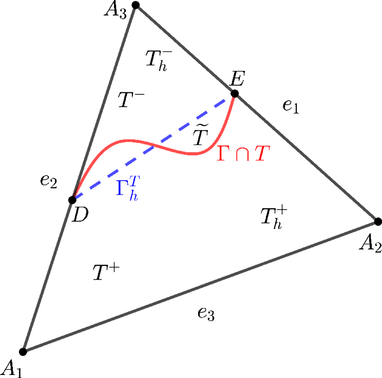
Assumption (A1) is fulfilled for a linear interface, and thus it should hold if a curved interface is locally flat enough, i.e., the mesh is fine enough. By the assumption (A1), we define
 $\Gamma^{T}_h$
as the line connecting the two intersection points of each interface element T, let
 $\Gamma^T_h$
cut T into two subelements
 $T^-_h$
,
 $T^+_h$
and let
 $\widetilde{T}$
be the subregion sandwiched by
 $\Gamma^T_h$
and
 $\Gamma$
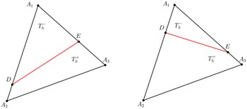
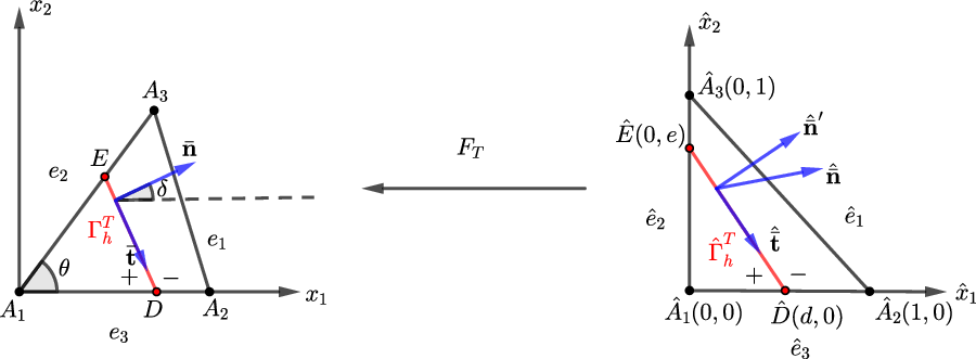
as shown in Figure 3. In addition,
 $T^-$
and
 $T^+$
refer to the subelements partitioned by the interface curve itself instead of its linear approximation
 $\Gamma^T_h$
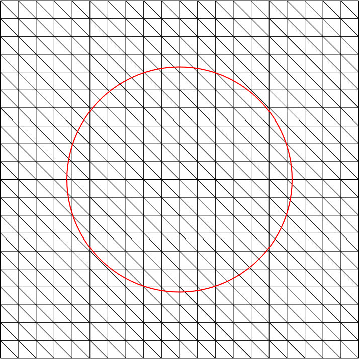
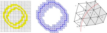
. For Assumption (A2), IFE methods can be and are often used on simple triangular Cartesian meshes as shown in Figure 2, especially for electromagnetic waves where computational domains are often truncated as boxes. So we can generate Cartesian meshes for computation which certainly satisfy Assumption (A2). In the following discussion, we shall focus on Cartesian meshes although most of the results are applicable to general triangulation unless otherwise specified. Assumption (A3) is only technically used for showing the inf-sup condition, see the details in Section 5.
An unfitted mesh.

An interface element.

Moreover, we assume the interface is well-resolved by the mesh, and it can be quantitatively described in terms of the following lemma [Reference Guo and Lin34].
Lemma 1. Suppose the mesh is sufficiently fine such that
 $h<h_0$
for some value
 $h_0$
, then on each interface element
 $T\in\mathcal{T}^i_h$
, for every two points
 $X_1,X_2\in\Gamma\cap T$
with their normal vectors
 $\mathbf{ n}(X_1),\mathbf{ n}(X_2)$
to
 $\Gamma$
and every point
 $X\in\Gamma\cap T$
with its orthogonal projection
 $X^{\bot}$
onto
 $\Gamma^T_h$
,
 \begin{equation}\| X-X^{\bot} \| \lesssim h_T^2 \,\,\, \text{and} \,\,\, \| \mathbf{ n}(X_1)-\mathbf{ n}(X_2) \| \lesssim h_T.\end{equation}
The explicit dependence of
 $h_0$
on the interface curvature can be found in [Reference Guo and Lin34].
Next we introduce some Sobolev spaces. For each subdomain
 $\omega\subseteq\Omega$
, we let
 $H^k(\omega)$
and
 $\textbf{H}^k(\omega)$
,
 $k\ge0$
, be the standard scalar and
 $\mathbb{R}^2$
-vector Hilbert spaces on
 $\omega$
; in particular
 $H^0(\omega)=L^2(\omega)$
and
 $\textbf{H}^0(\omega) =\textbf{L}^2(\omega)$
. In addition,
 \begin{equation} \textbf{H}^k(\text{curl};\,\omega) \,:\!=\, \left\{ \textbf{v}\in\textbf{H}^k(\omega)\,:\,\text{curl}\,\textbf{v} \in H^k(\omega) \right\}. \end{equation}
For simplicity, we shall drop “0" if
 $k=0$
; namely
 $\textbf{H}(\text{curl};\,\omega) = \textbf{H}^0(\text{curl};\,\omega)$
. If
 $|\omega\cap\Gamma|\neq 0$
, we let
 $\omega^{\pm}=\Omega^{\pm}\cap\omega$
and further define the broken space for
 $k\ge\frac{1}{2}$
as
 \begin{equation}\widetilde{\textbf{H}}^k(\text{curl};\,\omega) \,:\!=\, \left\{ \textbf{v}\in \textbf{L}^2(\omega)\,:\, \textbf{v}|_{\omega^{\pm}} \in \textbf{H}^k\left(\text{curl};\,\omega^{\pm}\right), \,\textbf{v}\, \text{satisfies the jump conditions in (1.1b)--(1.1d)} \right\}.\end{equation}
For all these spaces,
 $H^k_0(\omega)$
,
 $\textbf{H}^k_0(\omega)$
,
 $\textbf{H}^k_0(\text{curl};\,\omega)$
and
 $\widetilde{\textbf{H}}^k_0(\text{curl};\,\omega)$
denote the subspaces with the zero trace on
 $\partial \omega$
. The associated norms are denoted by
 $\|\cdot\|_{H^k(\omega)}$
,
 $\|\cdot\|_{L^2(\omega)}$
(here we do not distinguish
 $\|\cdot\|_{H^k(\omega)}$
and
 $\|\cdot\|_{\textbf{H}^k(\omega)}$
for standard Hilbert spaces for simplicity),
 $\|\cdot\|_{\textbf{H}(\text{curl};\,\omega)}$
and
 $\|\cdot\|_{\textbf{H}^1(\text{curl};\,\omega)}$
.
For discretisation, we shall employ the first family Nédélec element of the lowest degree [Reference Nedelec61]:
 \begin{align} \mathcal{ND}_h(T) & = \left\{ {\textbf{a}} + b[x_2,-x_1]^t\,: \, {\textbf{a}}\in\mathbb{R}^2, b\in\mathbb{R} \right\}, \nonumber\\[4pt] \mathcal{ND}_h(\Omega) & = \left\{ \textbf{v}\in\textbf{H}(\text{curl};\,\Omega)\,:\, \textbf{v}|_T \in \mathcal{ND}_h(T) \,\, \forall T\in\mathcal{T}_h \right\}. \end{align}
Let
 $\mathcal{ND}_{h,0}(\Omega)$
denote the subspace of
 $\mathcal{ND}_h(\Omega)$
with the zero trace on
 $\partial \Omega$
. On an element T, the space
 $\mathcal{ND}_h(T)$
can be equipped with the well-known edge interpolation operator [Reference Ciarlet and Zou25, Reference Monk60] denoted by
 $\Pi_{T}\,:\, \textbf{H}^1(\text{curl};\,T) \longrightarrow \mathcal{ND}_h(T)$
. Then the global interpolation operator
 $\Pi_h\,:\,\textbf{H}^1(\text{curl};\,\Omega)\rightarrow \mathcal{ND}_h(\Omega)$
can be defined in a usual piecewise manner. The following optimal approximation capabilities hold [Reference Ciarlet and Zou25, Reference Monk60]:
 \begin{equation}\| \textbf{u} - \Pi_{T}\textbf{u} \|_{\textbf{H}(\text{curl};\,T)} \lesssim h_T \| \textbf{u} \|_{\textbf{H}^1(\text{curl};\,T)}\,\,\,\, \text{and} \,\,\,\, \| \textbf{u} - \Pi_h\textbf{u} \|_{\textbf{H}(\text{curl};\,\Omega)} \lesssim h \| \textbf{u} \|_{\textbf{H}^1(\text{curl};\,\Omega)}.\end{equation}
In addition, we let
 $S_h(\Omega)\subset H^1(\Omega)$
be the continuous piecewise linear finite element space, and also define
 $I_h \,:\, H^2(\Omega)\rightarrow S_h(\Omega)$
as the standard nodal interpolation operator. Also let
 $S_{h,0}(\Omega)$
be the subspace of
 $S_h(\Omega)$
with the zero trace on
 $\partial \Omega$
.
Following [Reference Hiptmair, Li and Zou41], we make a more practical assumption than most existing studies for the exact solution to the interface problem (1), namely the piecewise smoothness
 $\textbf{u}\in \widetilde{\textbf{H}}^1_0(\text{curl};\,\Omega)$
. Given a convex domain
 $\Omega$
, such an assumption is satisfied when the interface is a smooth simple Jordan curve and does not touch the boundary [Reference Alberti3, Reference Costabel, Dauge and Nicaise26, Reference Huang and Zou49]. Even so, the estimate in (1.2) may make algorithms fail to converge. In more practical situations, weaker regularities may be produced by less smooth geometries, such as non-convex polygonal domains or non-smooth interfaces. In fact, with a Helmholtz decomposition, the singular part of
 $\textbf{u}$
can be expressed in the form of a gradient whose regularity may be worse due to the interface. We refer readers to Section 4.3 in [Reference Ben Belgacem, Buffa and Maday15] and Theorem 2 in [Reference Casagrande, Hiptmair and Ostrowski19] for the discussion about how the convergence of non-conforming methods can be affected by regularity. According to the tangential continuity jump condition, we note that
 $\widetilde{\textbf{H}}^1_0(\text{curl};\,\Omega)\subset\textbf{H}_0(\text{curl};\,\Omega)$
, and in particular we can further conclude
 $\widetilde{\textbf{H}}^1_0(\text{curl};\,\Omega)\subset\textbf{H}^s_0(\Omega)$
,
 $0\leqslant s<1/2$
, by Theorem 4.1 in [Reference Hiptmair40].
We are now ready to state the variational formulation of the system (1.1): find
 $\textbf{u} \in \textbf{H}_0(\text{curl};\,\Omega)$
such that
 \begin{equation}a(\textbf{u},\textbf{v}) = \int_{\Omega} \textbf{f}\cdot\textbf{v} dX \,\,\,\,\,\, \forall \textbf{v} \in \textbf{H}_0(\text{curl};\,\Omega),\end{equation}
where the bilinear form is given by
 \begin{equation}a(\textbf{u},\textbf{v}) = \int_{\Omega}\mu^{-1}\text{curl}\,\textbf{u}\cdot\text{curl}\,\textbf{v} dX + \int_{\Omega} \beta \textbf{u}\cdot\textbf{v} dX.\end{equation}
It naturally leads to an energy norm
 $\| \textbf{v} \|_a=a(\textbf{v},\textbf{v})^{\frac{1}{2}}$
, and it is easy to see
 $\| \cdot \|_a$
is equivalent to
 $\| \cdot \|_{\textbf{H}(\text{curl};\,\Omega)}$
.
We end this section by recalling an
 $\textbf{H}^1(\text{curl};\,\Omega)$
-extension operator [Reference Hiptmair, Li and Zou41, Theorem 3.4 and Corollary 3.5].
Theorem 2.1. There exist two bounded linear operators
 $\textbf{E}^{\pm}_{\textrm{curl}} \,:\, \textbf{H}^1(\textrm{curl};\,\Omega^{\pm})\rightarrow \textbf{H}^1(\textrm{curl};\,\Omega)$
, such that for each
 $\textbf{u}\in\textbf{H}^1(\textrm{curl};\,\Omega^{\pm})$
:
-
1.
$\textbf{E}^{\pm}_{\textrm{curl}}\textbf{u} = \textbf{u} \,\, \text{a.e.} \,\text{in} \, \Omega^{\pm}$
. -
2.
$\| \textbf{E}^{\pm}_{\textrm{curl}}\textbf{u} \|_{\textbf{H}^1(\textrm{curl};\,\Omega)} \leqslant C_E \| \textbf{u} \|_{\textbf{H}^1(\textrm{curl};\,\Omega^{\pm})}$
with the constant
$C_E$
only depending on
$\Omega^{\pm}$
.


Using these two special extension operators, we can define
 $\textbf{u}^{\pm}_E = \textbf{E}^{\pm}_{\text{curl}}\textbf{u}^{\pm}$
which are crucial to the following analysis.
3. IFE discretisation
In this section, we first develop the Nédélec-type IFE functions which are then used in a PG formulation to solve the
 $\textbf{H}(\text{curl})$
-elliptic interface problem. In addition, we will present an exact sequence that will be technically used in the stability analysis.
3.1. The edge IFE spaces
It is generally convenient and useful to consider an IFE function as an extension of one polynomial component to another. So given each interface element
 $T\in\mathcal{T}^i_h$
, we let
 $\bar{\textbf{t}}$
and
 $\bar{\textbf{n}}$
be the tangential and normal vectors to the segment
 $\Gamma^T_h$
. Then we consider a linear operator
 $\mathcal{C}_T\,:\, \mathcal{ND}_h\left(T^-_h\right)\rightarrow \mathcal{ND}_h(T^+_h)$
satisfying:
 \begin{align} \mathcal{C}_T(\textbf{v}_h)\cdot\bar{\textbf{t}} &= \textbf{v}_h \cdot\bar{\textbf{t}} \,\,\,\,\,\,\,\,\,\,\,\,\,\,\,\,\, \text{on} \, \Gamma^T_h, \end{align}
 \begin{align} \frac{1}{\mu^{+}}\text{curl}\,\mathcal{C}_T(\textbf{v}_h) & = \frac{1}{\mu^{-}}\text{curl}\,\textbf{v}_h \,\,\,\,\,\, \text{in} \, T, \end{align}
 \begin{align} \beta^+\mathcal{C}_T(\textbf{v}_h)\cdot\bar{\textbf{n}} &= \beta^- \textbf{v}_h \cdot\bar{\textbf{n}} \,\,\,\,\,\,\,\,\,\,\, \text{at} \, X_m,\end{align}
where
 $X_m=[x_{m,1},x_{m,2}]^t$
is a middle point of
 $\Gamma^T_h$
. But the approximate jump conditions in (3.1) may be imposed at any point at
 $\Gamma^{T}_h$
, and we choose the midpoint
 $X_m$
for simplifying the derivation. This linear operator is not only well defined but also bijective, which is valid for both
 $T_h^-$
and
 $T_h^+$
being of general polygonal shape. It does not affect our subsequent analysis if
 $\mathcal{C}_T$
is defined the other way around, i.e., from
 $\mathcal{ND}_h(T^+_h)$
to
 $\mathcal{ND}_h\left(T^-_h\right)$
. In particular, we can establish the explicit format for the operator
 $\mathcal{C}_T$
. Let us denote
 $X=[x_1,x_2]^t\in\mathbb{R}^2$
, let D be one intersection point of
 $\Gamma$
and
 $\partial T$
shown in Figure 3 and take the rotation matrix
 $\textbf{R}=[0,1;\,-1,0]$
, then
 \begin{equation}\begin{split}&\mathcal{C}_T(\textbf{v}_h) = \textbf{v}_h + b_1 \textbf{R} \left[ X -D \right] + b_2 \bar{\textbf{n}} , \,\,\,\,\, \forall \textbf{v}_h\in \mathcal{ND}_h\left(T^-_h\right), \\\text{with} \,\, & b_1 = \frac{1}{2}\left( 1- \frac{\mu^+}{\mu^-} \right) \text{curl}\,\textbf{v}_h \,\,\, \text{and} \,\,\, b_2 = \left( \frac{\beta^-}{\beta^+} - 1 \right) \textbf{v}_h(X_m)\cdot\bar{\textbf{n}} - \frac{b_1|\Gamma^T_h|}{2}.\end{split}\end{equation}
One can immediately verify that the linear mapping in (3.2) satisfies (3.1) and is bijective. This mapping will be useful in both the analysis of approximation capabilities and trace inequalities.
Furthermore, we have simple formulas for the IFE functions satisfying (3.1). Define a transformation matrix
 \begin{equation*}M_T = [\bar{\textbf{n}},\bar{\textbf{t}}] \left[\begin{array}{c@{\quad}c} \beta^-/\beta^+ & 0 \\[4pt] 0 & 1 \end{array}\right][\bar{\textbf{n}},\bar{\textbf{t}}]^t, \end{equation*}
and a piecewise constant vector space
 ${\textbf{C}}_h(T) = \{ {\textbf{a}}|_{T^{\pm}_h} \in \mathbb{R}^2\,:\, {\textbf{a}}|_{T^{+}_h} = M_T{\textbf{a}}|_{T^{-}_h}\}$
. Then we can define the local IFE space on each interface element as
 \begin{equation}\mathcal{IND}_h(T) = \{ \textbf{z}_h\,:\, \textbf{z}_h= \mu b [(x_2-x_{m,2}),-(x_1-x_{m,1})]^t + {\textbf{a}}, \,\,\, \forall b\in\mathbb{P}_0(T), \, {\textbf{a}}\in {\textbf{C}}_h(T)\}.\end{equation}
Note that the format is close to the standard Nédélec functions in (2.4) where the only difference is on the piecewise-defined constants (vectors). Also, there holds
 $\text{dim}(\mathcal{IND}_h(T))=3$
which is identical to the standard one. Besides, one can verify that
 $\textbf{z}_h$
in (3.3) satisfies
 $\textbf{z}^+_h = \mathcal{C}_T(\textbf{z}^-_h)$
. Hence, by (3.1a), we can see
 $\mathcal{IND}_h(T) \subset \textbf{H}(\text{curl};\,T)$
, but
 $\mathcal{IND}_h(T) \not\subset \textbf{H}^1(\text{curl};\,T)$
due to (3.1b).
Remark 3.1. From (3.2), it is not hard to see that both
 $b_1$
and
 $b_2$
will vanish if
 $\mu^-=\mu^+$
and
 $\beta^-=\beta^+$
. In this case,
 $\mathcal{C}_T$
reduces to an identity operator, and thus the proposed IFE functions are consistent with standard Nédélec functions. This feature is particularly useful for moving interface problems.
Next, to construct suitable global IFE spaces, it is important to select local basis functions in
 $\mathcal{IND}_h(T)$
with the edge degrees of freedom (DoFs) since they can match the standard Nédélec spaces, and thus the edge DoFs can glue the IFE functions on interface elements with the Nédélec functions on the surrouding non-interface elements. In particular, for an element T with the edges
 $e_i$
and the corresponding tangential vectors
 $\textbf{t}_i$
,
 $i=1,2,3$
, we impose the DoFs for functions in
 $\mathcal{IND}_h(T)$
:
 \begin{equation}\int_{e_i} \textbf{z}\cdot\textbf{t}_i ds = v_i, \,\,\,\, i=1,2,3\end{equation}
with some values
 $v_i\in\mathbb{R}$
. The unisolvence is established in the following theorem.
Theorem 3.1. (Unisolvence) Suppose that T does not have an obtuse angle, then the DoFs (3.4) are unisolvent on
 $\mathcal{IND}_h(T)$
regardless of the interface location or the parameters
 $\mu$
and
 $\beta$
.
Proof. See Appendix A.1
Theorem 3.1 guarantees the existence of local IFE shape functions by taking
 $v_i$
to be 0 or 1 in (3.4), namely there exist
 $\boldsymbol{\psi}_{T,i}\in\mathcal{IND}_h(T)$
such that
 $\int_{e_j} \boldsymbol{\psi}_{T,i}\cdot\textbf{t}_j ds = \delta_{ij}$
,
 $i,j =1,2,3$
. Then the local IFE space (3.3) can be rewritten as
 \begin{equation}\mathcal{IND}_h(T) = \text{Span}\{ \boldsymbol{\psi}_{T,1}, \boldsymbol{\psi}_{T,2}, \boldsymbol{\psi}_{T,3} \}.\end{equation}
We also provide the detailed construction approach of IFE shape functions in Appendix A.1. Furthermore, we can prove the following properties of these shape functions.
Theorem 3.2. Suppose that T does not have an obtuse angle and is shape regular, then for
 $i=1,2,3$
there hold
 \begin{align} & \| \boldsymbol{\psi}_{T,i} \|_{L^{\infty}(T)} \lesssim h^{-1}_T, \end{align}
 \begin{align}& \mu^{-1}\textrm{curl}\,\boldsymbol{\psi}_{T,i} = 2 (|T^-|\mu^- + |T^+|\mu^+ )^{-1} \lesssim h^{-2}_T. \end{align}
Proof. See Appendix A.2.
Remark 3.2. Theorem 3.1 means that the unisolvence always holds regardless of interface location and the parameters
 $\beta$
,
 $\mu$
if the maximal angle is not greater than
 $\pi/2$
. Besides, if the maximal angle is close or equal to
 $\pi/2$
, the constants in Theorem 3.2 do not blow up. But for an obtuse triangle, it is possible to find some interface configuration and
 $\beta$
,
 $\mu$
to violate the unisolvence, and in this case, the constants in Theorem 3.2 may blow up.
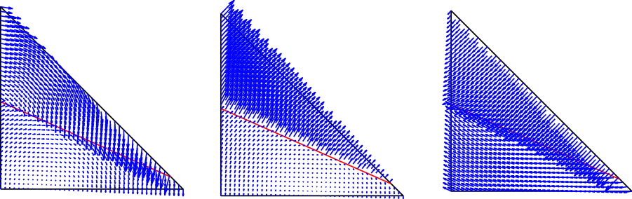
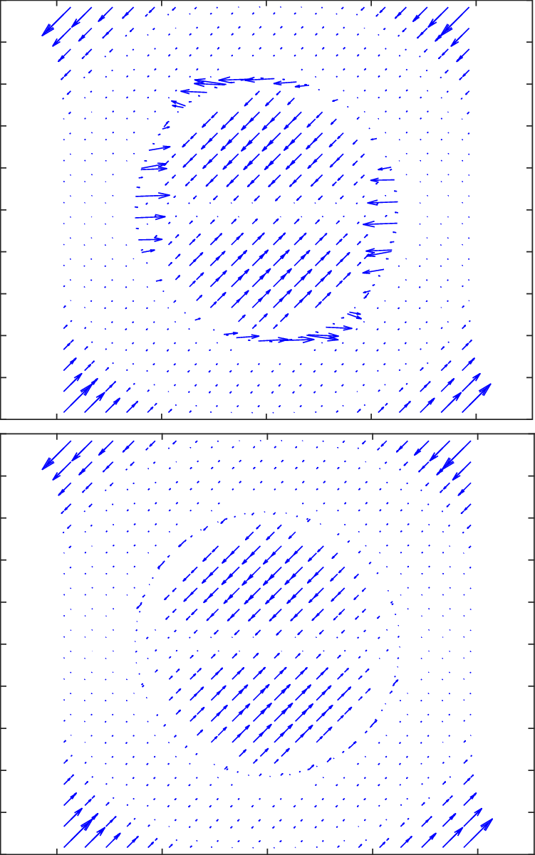
Here, we plot some examples of IFE shape functions, i.e.,
 $\boldsymbol{\psi}_{T,i}$
constructed above, in Figure 4 where the interface is the red line and the parameters for the media below and above the interface are
 $(\mu,\beta)=(1/2,1)$
and (1,10), respectively. We see that the vector fields are discontinuous across the interface.
IFE shape functions associated with each edge of an interface element.

As usual, the local IFE spaces on non-interface elements are simply defined as the standard Nédélec spaces
 $\mathcal{IND}_h(T)=\mathcal{ND}_h(T)$
. Hence, we can define the global IFE space:
 \begin{equation}\mathcal{IND}_h(\Omega) = \bigg\{ \textbf{v}\in \textbf{L}^2(\Omega)\,:\, \textbf{v}|_T \in \mathcal{IND}_h(T) \,\, \forall T\in\mathcal{T}_h, \,\, \int_e [\textbf{v}\cdot\textbf{t}]_e ds =0 \,\, \forall e\in{\mathop{\mathcal{E}}\limits^{\tiny\circ}}_h \bigg\}.\end{equation}
Let
 $\mathcal{IND}_{h,0}(\Omega)$
be the subspace with the zero trace on
 $\partial \Omega$
. In addition, we mimic the standard edge interpolation to define a similar one for the IFE space
 $\mathcal{IND}_h(\Omega)$
:
 \begin{equation}\begin{split}\widetilde{\Pi}_h\,:\, \widetilde{\textbf{H}}^1(\text{curl};\,\Omega) \longrightarrow \mathcal{IND}_h(\Omega) \,\, \text{with} \,\, \int_e \widetilde{\Pi}_h\textbf{u}\cdot\textbf{t} ds = \int_e \textbf{u}\cdot\textbf{t} ds, \,\, \forall e\in\mathcal{E}_h.\end{split}\end{equation}
Again we have the local interpolation
 $\widetilde{\Pi}_{T}=\widetilde{\Pi}_h|_T$
for each element T.
3.2. A Petrov–Galerkin IFE scheme
The proposed PG-IFE scheme relies on the isomorphism between
 $\mathcal{IND}_h(\Omega)$
and
 $\mathcal{ND}_h(\Omega)$
, as the resulting linear system needs to be square. The isomorphism can be described by an operator
 $\mathbb{\Pi}_h\,:\,\mathcal{IND}_h(\Omega) \longrightarrow \mathcal{ND}_h(\Omega)$
defined in the same manner as the interpolation due to the edge DoFs. We note that
 $\mathbb{\Pi}_h$
can be understood as the interpolation operator
 $\Pi_h$
applied to the space
 $\mathcal{IND}_h(\Omega)$
, while
 $\mathbb{\Pi}^{-1}_h$
can be understood as
 $\widetilde{\Pi}_h$
in (3.8) applied to the space
 $\mathcal{ND}_h(\Omega)$
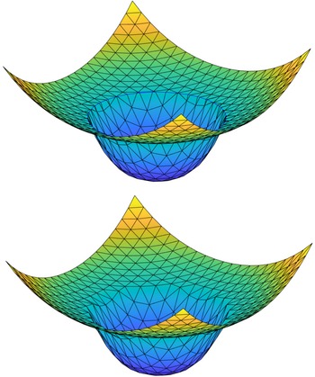
. To show how IFE functions are related to their FE counterparts through
 $\mathbb{\Pi}_h$
, here we plot an example of the vector field in Figure 5 where clearly they are identical except at the interface.
A global
 $\textbf{H}(\text{curl})$
IFE function and its FE isomorphic image.

Then the PG-IFE scheme is to find
 $\textbf{u}_h\in \mathcal{IND}_{h,0}(\Omega)$
such that
 \begin{equation}a(\textbf{u}_h,\textbf{v}_h) = \int_{\Omega} \textbf{f}\cdot\textbf{v}_h \, dX \,\,\,\,\,\, \forall \textbf{v}_h\in \mathcal{ND}_{h,0}(\Omega),\end{equation}
where the bilinear form is defined in (2.7). Although the local IFE spaces
 $\mathcal{IND}_h(T)$
are subspaces of
 $\textbf{H}(\text{curl};\,T)$
, the global space in (3.7) is not
 $\textbf{H}(\text{curl})$
-conforming. To see this, we note that
 $\int_e [\textbf{v}_h\cdot\textbf{t}]_e ds =0$
does not lead to
 $[\textbf{v}_h\cdot\textbf{t}]_e =0$
since
 $\textbf{v}_h\cdot\textbf{t}$
is not a constant on e. As mentioned before, this non-conformity widely appears in many interface-unfitted methods either on element boundary [Reference Guo and Lin34, Reference Lin, Lin and Zhang55] or on the interface itself [Reference Burman, Claus, Hansbo, Larson and Massing17, Reference Huang, Wu and Xiao50]. Penalties are usually used to handle it for both consistency and stability such that optimal convergence can be obtained. Due to the reason described in the introduction, the penalty is troublesome for
 $\textbf{H}(\text{curl})$
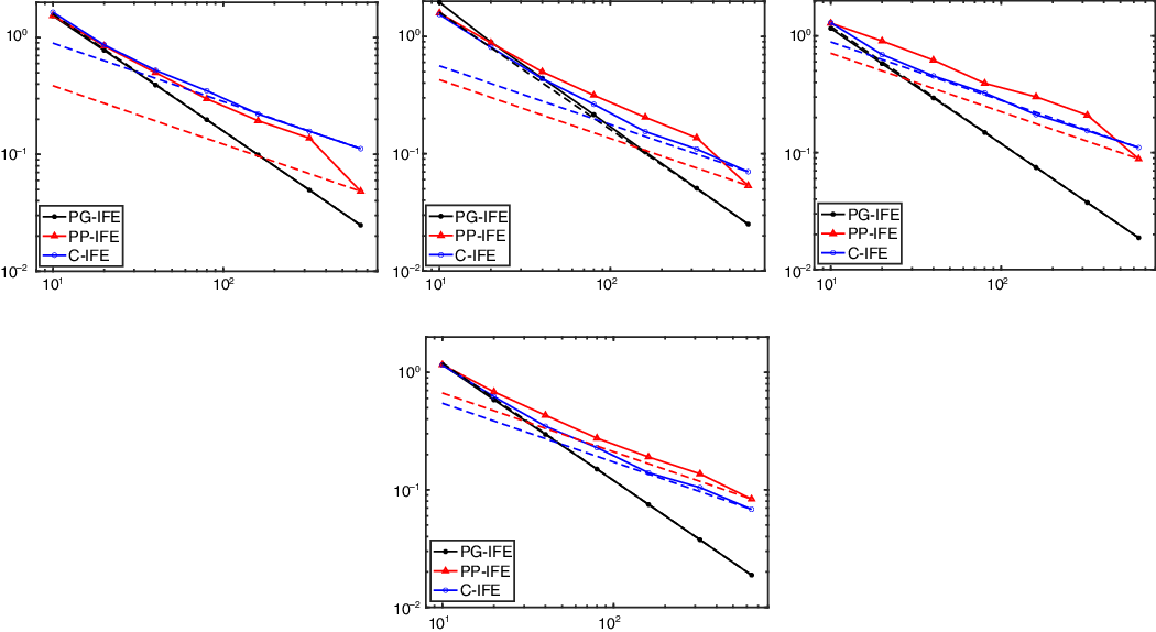
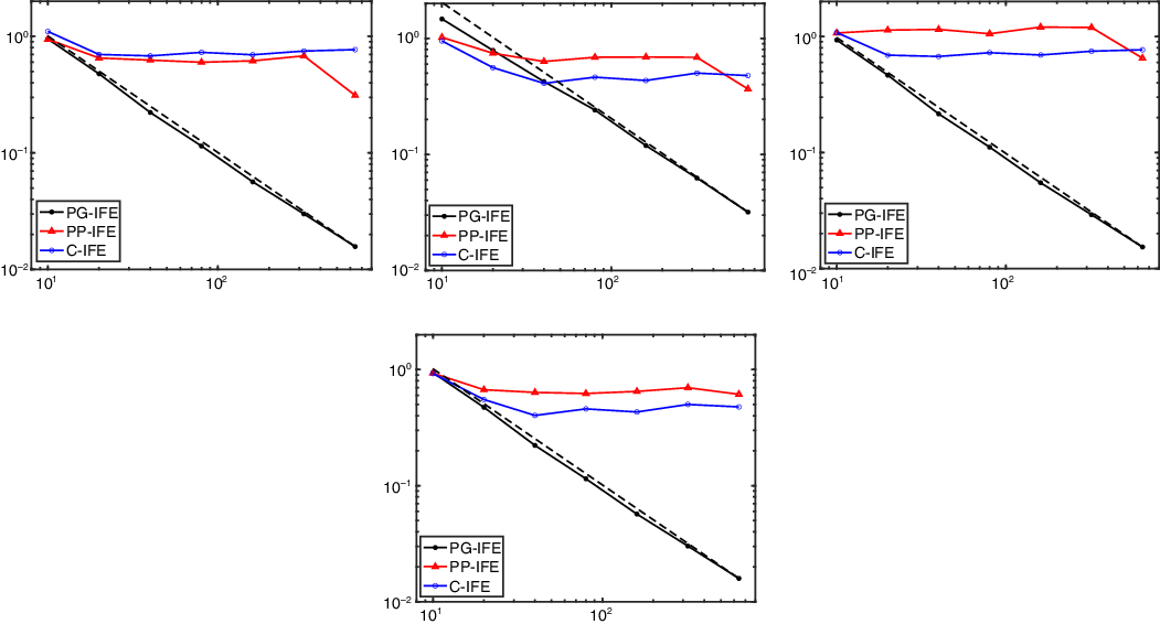
problems. Indeed, for the IFE method, numerical results in Section 6 indicate that solutions of the penalty-type scheme or the standard Galerkin scheme do not converge at all near the interface.
3.3. Characterisation of immersed elements
In this subsection, we follow the spirit of the well-known de Rham complex [Reference Arnold, Falk, Winther, Arnold, Bochev, Lehoucq, Nicolaides and Shashkov6] to derive some analogue properties for the IFE spaces, which is the foundation in the analysis of the inf-sup stability in Section 5.
We first recall the
 $H^1$
immersed elements in the literature [Reference Guo and Lin34, Reference Li, Lin, Lin and Rogers53]. The scalar solution
 $u^{\pm}\,:\!=\,u|_{\Omega^{\pm}}$
of the
 $H^1$
-elliptic interface problem should satisfy the jump conditions at the interface:
 \begin{equation}u^+ = u^- \,\,\,\, \text{and} \,\,\,\, \beta^+ \nabla u^+\cdot\textbf{n} = \beta^- \nabla u^-\cdot\textbf{n} \,\,\, \text{on} \, \Gamma,\end{equation}
where
 $\beta^{\pm}$
are assumed to be the same as those in (1.1), i.e., conductivity in physics. We define the Sobolev space
 \begin{equation*}\widetilde{H}^2_0(\Omega)= \left\{ v \in H^1(\Omega)\,:\, v|_{\Omega^{\pm}}\in H^2_0(\Omega^{\pm})\, \text{and}\, v\,\text{satisfies the jump conditions in (3.10)} \right\} .\end{equation*}
Then the local
 $H^1$
IFE space on each interface element, i.e., the one shown in Figure 3, is defined as
 \begin{equation}\widetilde{S}_h(T) = \{ z_h\,:\, z^{\pm}_h= z_h|_{T^{\pm}_h}\in \mathbb{P}_1(T^{\pm}_h),\, z^+_h=z^-_h, \,\, \beta^-\nabla z^-_h\cdot\bar{\textbf{n}} = \beta^+\nabla z^+_h\cdot\bar{\textbf{n}} \,\, \text{on} \, \Gamma^T_h \}.\end{equation}
Clearly there holds
 $\widetilde{S}_h(T)\subset H^1(T)$
, and one can pick shape functions from
 $\widetilde{S}_h(T)$
with the nodal value DoFs. Then, we let
 $\widetilde{S}_h(\Omega)$
be a global IFE space continuous at the mesh nodes, and let
 $\widetilde{S}_{h,0}(\Omega)$
be the zero-trace subspace. There generally holds
 $\widetilde{S}_h(\Omega)\subsetneq H^1(\Omega)$
due to the discontinuities across interface edges, but the nodal DoFs still enable us to define the nodal interpolation
 $\tilde{I}_h$
. We refer readers to [Reference Li, Lin, Lin and Rogers53] for more details.
 \begin{equation}\left.\begin{array}{ccc}H^2_0(\Omega) & \xrightarrow[]{\,\,\nabla\,\,} & \textbf{H}^1_0(\text{curl};\,\Omega) \\\,\,\,\,\bigg\downarrow I_{h} & & \,\,\,\,\bigg\downarrow \Pi_{h} \\S_{h,0}(\Omega) & \xrightarrow[]{\,\,\nabla\,\,} & \mathcal{ND}_{h,0}(\Omega)\end{array}\right.\,\,\,\left.\begin{array}{ccc}\widetilde{H}^2_0(\Omega) & \xrightarrow[]{\,\,\nabla\,\,} & \widetilde{\textbf{H}}^1_0(\text{curl};\,\Omega) \\\,\,\,\,\bigg\downarrow \tilde{I}_{h} & & \,\,\,\,\bigg\downarrow \tilde{\Pi}_{h} \\\widetilde{S}_{h,0}(\Omega) & \xrightarrow[]{\,\,\nabla\,\,} & \mathcal{IND}_{h,0}(\Omega)\end{array}\right.\end{equation}
According to the well-known de Rham complex [Reference Arnold, Falk, Winther, Arnold, Bochev, Lehoucq, Nicolaides and Shashkov6, Reference Arnold, Falk and Winther7], we plot the diagram for
 $H^2_0(\Omega)$
and
 $\textbf{H}^1_0(\text{curl};\,\Omega)$
spaces in the left of (3.12) which is commutative. The IFE spaces share the similar property shown by the right plot in (3.12) where the gradient
 $\nabla$
is understood element-wisely. Here, we note that functions in
 $\nabla\widetilde{H}^2_0(\Omega)$
satisfy the jump conditions (1.1b) and (1.1d) because of (3.10) and satisfy (1.1c) because they are curl-free, and thus
 $\nabla\widetilde{H}^2_0(\Omega)\subseteq\widetilde{\textbf{H}}^1_0(\text{curl};\,\Omega)$
. The next lemma shows this new diagram is well-defined.
Lemma 2. For IFE spaces, there holds
 $\nabla \widetilde{S}_{h,0}(\Omega) \subseteq \mathcal{IND}_{h,0}(\Omega)$
.
Proof. The local results
 $\nabla\widetilde{S}_h(T)\subset \mathcal{IND}_h(T)$
are trivial due to the jump conditions. The global result is non-trivial due to the discontinuities on interface edges. For each interface edge
 $e\in\mathcal{E}_h$
, we need to show
 $\int_e[\nabla v_h\cdot\textbf{t}_e]ds=0$
,
 $v_h\in \widetilde{S}_{h}(\Omega)$
. Let
 $A_1$
and
 $A_2$
be the two nodes of e, let
 $\textbf{t}_e$
be oriented from
 $A_1$
to
 $A_2$
and let
 $T_1$
and
 $T_2$
be its neighbour elements. Then the continuity at the interface intersection point of e yields
 \begin{equation}\int_e \nabla v_h|_{T_1}\cdot \textbf{t}_e ds = \int_e \partial_{\textbf{t}_e} v_h|_{T_1} ds = v_h|_{T_1}(A_1) - v_h|_{T_1}(A_2).\end{equation}
A similar identity also holds for
 $T_2$
. Therefore, the continuity at mesh nodes yields the desired result.
The next result is for the commuting property of IFE spaces.
Theorem 3.3. The diagram on the right of (3.12) is commutative, namely
 $\widetilde{\Pi}_h \circ \nabla = \nabla \circ \tilde{I}_h$
,
 $\text{on} \, \widetilde{H}^2_0(\Omega)$
.
Proof. The result is trivial on non-interface elements, and, on interface elements, it follows from the argument similar to (3.13) and the nodal continuity of
 $\tilde{I}_{h} v$
and
 $v\in\widetilde{H}^2_0(\Omega)$
.
To show the exactness, we also need the isomorphism
 $\mathbb{I}_h\,:\,S_h(\Omega)\rightarrow \widetilde{S}_h(\Omega)$
that is defined in the same manner as the usual nodal interpolation. Similarly,
 $\mathbb{I}_h$
can be understood as
 $I_h$
applied to
 $\widetilde{S}_h(\Omega)$
and
 $\mathbb{I}^{-1}_h$
can be understood as
 $\tilde{I}_h$
applied to
 $S_h(\Omega)$
. The new notations
 $\mathbb{I}_h$
and
 $\mathbb{\Pi}_h$
are just used to emphasise the isomorphism. Here, we also plot an
 $H^1$
IFE function and its FE isomorphic image in Figure 6.
A global
 $H^1$
IFE function and its FE isomorphic image.

Remark 3.3. By similar arguments to Theorem 3.3, the following commuting properties also hold
 \begin{equation}\mathbb{\Pi}_h \circ\nabla = \nabla \circ \mathbb{I}_h \,\,\, \text{on} \, \widetilde{S}_{h,0}(\Omega) \,\,\,\,\, \text{and} \,\,\,\,\, \mathbb{\Pi}^{-1}_h \circ\nabla = \nabla \circ \mathbb{I}^{-1}_h \,\,\, \text{on} \, S_{h,0}(\Omega).\end{equation}
Furthermore, we can show that
 $\mathbb{\Pi}_h$
yields an isomorphism between
 $\text{Ker(curl)}\cap\mathcal{IND}_{h,0}(\Omega)$
and
 $\text{Ker(curl)}\cap\mathcal{ND}_{h,0}(\Omega)$
.
Theorem 3.4.
 $\mathbb{\Pi}_h$
is an isomorphism between
 $\textrm{Ker(curl)}\cap\mathcal{IND}_{h,0}(\Omega)$
and
 $\textrm{Ker(curl)}\cap\mathcal{ND}_{h,0}(\Omega)$
.
Proof. Let us focus on an interface element T, and recall that
 $\boldsymbol{\psi}_i$
,
 $i=1,2,3$
, are the
 $\textbf{H}(\text{curl})$
IFE shape functions. By the identity in (3.6b), we let
 $\tau=\mu^{-1}\text{curl}\,\boldsymbol{\psi}_i$
,
 $i=1,2,3$
. For each
 $\textbf{z}_h\in \mathcal{ND}_{h,0}(\Omega)$
, we note that
 $\mu^{-1}\text{curl}\, \mathbb{\Pi}^{-1}_{h} \textbf{z}_h$
is a constant, and then the integration by parts yields
 \begin{equation}\begin{split}\mu^{-1} \text{curl}\, \mathbb{\Pi}^{-1}_{h} \textbf{z}_h = \sum_{i=1}^3 \int_{e_i} \textbf{z}_h\cdot\textbf{t}_i ds \mu^{-1} \text{curl}\, \boldsymbol{\psi}_i = \int_{\partial T} \textbf{z}_h\cdot\textbf{t} \tau ds = \int_T \text{curl}\,\textbf{z}_h dX \,\tau = |T| \tau \text{curl}\,\textbf{z}_h.\end{split}\end{equation}
The identity above shows that
 $\text{curl}\,\textbf{z}_h=0$
if and only if
 $ \text{curl}\, \mathbb{\Pi}^{-1}_{h} \textbf{z}_h = 0$
, and similar results also hold on non-interface elements. Thus, we have the desired result.
Remark 3.4. We note that
 $\text{Ker(curl)}\cap\mathcal{ND}_{h,0}(\Omega)$
and
 $\text{Ker(curl)}\cap\mathcal{IND}_{h,0}(\Omega)$
consist of piecewise constant vectors but functions of the latter one on interface elements are piecewise constant vectors on each subelement. If
 $\beta^-=\beta^+$
, then the piecewise constant vector on each interface element will reduce to a single constant vector. Therefore, by the self-preserving property of
 $\mathbb{\Pi}_h$
, there holds
 $\mathbb{\Pi}_h|_{\textrm{Ker(curl)}\cap\mathcal{IND}_{h,0}(\Omega)} = \mathcal{I}$
where
 $\mathcal{I}$
is the identity.
Theorem 3.5. For the IFE spaces, the sequence
 $\widetilde{S}_{h,0}(\Omega)\xrightarrow[]{\nabla} \mathcal{IND}_{h,0}(\Omega) \xrightarrow[]{\textrm{curl}}Q_h$
is exact, where
 $Q_h\subset L^2(\Omega)$
is a piecewise constant space, namely
 \begin{equation}\nabla \widetilde{S}_{h,0}(\Omega) = \textrm{Ker(curl)}\cap\mathcal{IND}_{h,0}(\Omega) = \{ \textbf{z}_h\in \mathcal{IND}_{h,0}(\Omega)\,:\, \textrm{curl}\,\textbf{z}_h = 0\}.\end{equation}
Proof. By Lemma 2, it is easy to see
 $\nabla \widetilde{S}_{h,0}(\Omega)\subset \text{Ker(curl)}\cap\mathcal{IND}_{h,0}(\Omega)$
. As for the reverse direction, for each
 $\textbf{z}_h\in\text{Ker(curl)}\cap\mathcal{IND}_{h,0}(\Omega)$
, Theorem 3.4 suggests
 ${\Pi}_h\textbf{z}_h\in\text{Ker(curl)}\cap\mathcal{ND}_{h,0}(\Omega)$
. Then, due to the exact sequence for
 $S_{h,0}(\Omega)$
and
 $\mathcal{ND}_{h,0}(\Omega)$
, there exists
 $s_h\in S_{h,0}(\Omega)$
such that
 $\nabla s_h = \mathbb{\Pi}_h\textbf{z}_h$
. Now we take
 $\tilde{s}_h=\mathbb{I}^{-1}_hs_h$
and use (3.14) to obtain
 $\nabla \tilde{s}_h = \nabla \mathbb{I}^{-1}_h s_h = \mathbb{\Pi}^{-1}_h \nabla s_h = \mathbb{\Pi}^{-1}_h \mathbb{\Pi}_h\textbf{z}_h = \textbf{z}_h$
which has finished the proof.
4. Approximation capabilities
In this section, we analyse approximation capabilities of the IFE space (3.7) through the interpolation
 $\widetilde{\Pi}_h$
in (3.8). We shall first define a quasi interpolation to handle the jump condition, which will then be used to estimate the edge interpolation. The main difficulty is on interface elements due to the insufficient regularity of IFE functions.
4.1. A special quasi-interpolation
We introduce a patch
 $\omega_T$
for an element T:
 \begin{equation}\omega_T = \cup\{ T^{\prime}\in\mathcal{T}_h\,:\, T^{\prime}\cap T \neq \emptyset \}.\end{equation}
Then for each
 $T\in\mathcal{T}^i_h$
, we define its fictitious element:
 \begin{equation}T_{\epsilon} = \left\{ X\in\mathbb{R}^2\,:\,\exists Y\in T \, \text{s.t.}\, \overrightarrow{O_TX}=\epsilon\overrightarrow{O_TY} \right\},\end{equation}
where
 $O_T$
is the homothetic centre which can be simply chosen as the centroid of T, and
 $\epsilon\ge1$
is a scaling factor. In the following analysis, we assume there exists a fixed
 $\epsilon_0>1$
such that for each T there holds
 $T_{\epsilon_0}\subseteq \omega_T$
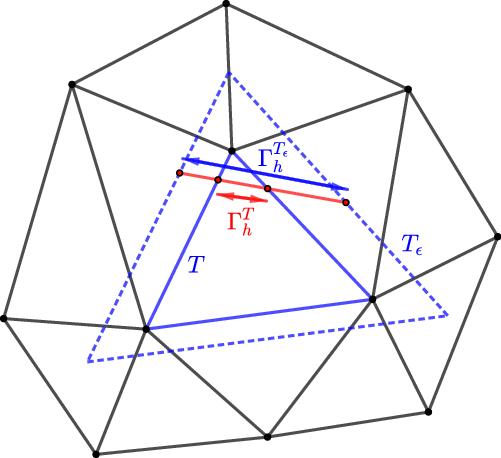
. It is easy to see that this assumption is fulfilled if the mesh is regular, see the illustration in Figure 7. Without loss of generality, from now on we shall fix
 $\epsilon=\epsilon_0$
for all fictitious elements. The reason for using fictitious elements is that each subelement of
 $T_{\epsilon}$
has a regular shape; namely, the inscribed ball has a lower bounded radius. We refer readers to Lemma 3.2 in [Reference Guo and Lin35] for more details. This property is important for making those generic constants in error estimates independent of interface location. In particular, we let
 $\Gamma^{T_{\epsilon}}_h$
be the extension of the straight line
 $\Gamma^T_h$
to
 $T_{\epsilon}$
, see Figure 7 for an illustration, and there holds for some uniform
 $\delta$
independent of interface location such that
 \begin{equation}|\Gamma^{T_{\epsilon}}_h| \ge \delta h_T. \end{equation}
A fictitious element and a patch.

Now we are ready to define the special interpolation operator
 \begin{equation}\begin{split}J_{T}\,:\, \widetilde{\textbf{H}}^1(\text{curl};\,T_{\epsilon}) \longrightarrow \mathcal{IND}_h(T_{\epsilon}) \,\,\,\, \text{with} \,\,\,\, J_{T} \textbf{u} = \begin{cases} J^-_{T} \textbf{u} = \Pi_{T_{\epsilon}} \textbf{u}^-_E \,\,\,\,\,\,\,\,\,\,\,\,\,\,\,\, \text{in} \, T^-_{\epsilon}, \\[5pt] J^+_{T} \textbf{u} = \mathcal{C}_T\left(\Pi_{T_{\epsilon}} \textbf{u}^-_E\right) \,\,\,\,\, \text{in} \, T^+_{\epsilon} ,\end{cases}\end{split}\end{equation}
where
 $\Pi_{T_{\epsilon}} \textbf{u}^-_E$
is a polynomial on
 $T_{\epsilon}$
but restricted onto
 $T^-$
to apply
 $\mathcal{C}_T$
. In fact, since polynomials can be naturally extended to everywhere, in the following analysis we always use
 $\Pi_{T_{\epsilon}} \textbf{u}^-_E$
,
 $\mathcal{C}_T\left(\Pi_{T_{\epsilon}} \textbf{u}^-_E\right)$
(those polynomials defined on subelements) on the whole
 $T_{\epsilon}$
. Here, it is worthwhile to mention that
 $\mathcal{ND}_h(T^{\pm})$
,
 $\mathcal{ND}_h(T^{\pm}_{\epsilon})$
and
 $\mathcal{ND}_h(T_{\epsilon})$
are the same polynomial spaces but defined on different region. We shall only use
 $\mathcal{ND}_h(T_{\epsilon})$
to denote the Nédélec space associated with both T and
 $T_{\epsilon}$
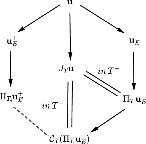
for simplicity. The motivation behind the special interpolation operator (4.4) is a relation connecting different extension and interpolation operators including
 $\textbf{E}^{\pm}_{\text{curl}}$
,
 $\mathcal{C}_T$
, and
 $\Pi_{T_{\epsilon}}$
, illustrated by the diagram in Figure 8. It suggests a delicate decomposition of the interpolation error
 $J_{T}\textbf{u}-\textbf{u}$
into the errors of
 $\Pi_{T_{\epsilon}}\textbf{u}^{\pm}_E - \textbf{u}^{\pm}_E$
and the error from
 $\mathcal{C}_T$
which is specifically denoted as
 \begin{equation}\boldsymbol{\eta}_h \,:\!=\, \Pi_{T_{\epsilon}}\textbf{u}^+_E - \mathcal{C}_T(\Pi_{T_{\epsilon}}\textbf{u}^-_E) \in \mathcal{ND}_h(T_{\epsilon}) .\end{equation}
The error
 $\boldsymbol{\eta}_h$
will be the main concern in the analysis below. Its estimation relies on a specially designed norm (4.6) that is constructed from the jump conditions:
 \begin{equation}\vert\kern-1pt\vert\kern-1pt\vert \textbf{v}_h \vert\kern-1pt\vert\kern-1pt\vert^2_{T_{\epsilon}} = h_T | \textbf{v}_h(X_m)\cdot\bar{\textbf{n}} |^2 + \| \textbf{v}_h\cdot\bar{\textbf{t}} \|^2_{L^2\left(\Gamma^{T_{\epsilon}}_h\right)} + \| \text{curl}\,\textbf{v}_h \|^2_{L^2\left(\Gamma^{T_{\epsilon}}_h\right)}, \,\,\, \forall \textbf{v}_h\in\mathcal{ND}_h(T_{\epsilon}).\end{equation}
The diagram for interpolation errors.

Lemma 3. The norm equivalence
 $h_T^{1/2}\vert\kern-1pt\vert\kern-1pt\vert\cdot\vert\kern-1pt\vert\kern-1pt\vert_{T_{\epsilon}}\simeq \|\cdot\|_{\textbf{H}(\textrm{curl};\,T_{\epsilon})}$
holds on
 $\mathcal{ND}_h(T_{\epsilon})$
where the constants in the equivalence relation are independent of interface location.
Proof. Given each
 $\textbf{v}_h\in\mathcal{ND}_h(T_{\epsilon})$
, since
 $\textbf{v}_h$
is simply a polynomial, using (4.3), the trace inequality and the inverse inequality, we have
 \begin{equation*}\begin{split}& h^{1/2}_T |\textbf{v}_h(X_m)\cdot\bar{\textbf{n}} | \leqslant \|\textbf{v}_h\cdot\bar{\textbf{n}} \|_{L^2\left(\Gamma^{T_{\epsilon}}_h\right)} \lesssim h^{-1/2}_T \| \textbf{v}_h \|_{L^2(T_{\epsilon})}, \\&\| \textbf{v}_h \cdot\bar{\textbf{t}} \|_{L^2\left(\Gamma^{T_{\epsilon}}_h\right)} \lesssim h_T^{-1/2}\| \textbf{v}_h \|_{L^2(T_{\epsilon})}, \,\,\, \| \text{curl} \, \textbf{v}_h \|_{L^2\left(\Gamma^{T_{\epsilon}}_h\right)} \lesssim h_T^{-1/2} \| \text{curl} \, \textbf{v}_h \|_{L^2(T_{\epsilon})}.\end{split}\end{equation*}
This yields
 $\vert\kern-1pt\vert\kern-1pt\vert\textbf{v}_h\vert\kern-1pt\vert\kern-1pt\vert_{T_{\epsilon}} \lesssim h^{-1/2}_T \| \textbf{v}_h \|_{\textbf{H}(\text{curl};\,T_{\epsilon})}$
. For the reverse direction, by the Taylor expansion, we have
 \begin{equation}\textbf{v}_h(X) = \textbf{v}_h(X_m) + \nabla \textbf{v}_h(X_m)(X-X_m) = \textbf{v}_h(X_m)\cdot\bar{\textbf{n}} + \textbf{v}_h(X_m)\cdot\bar{\textbf{t}} - \frac{1}{2}\text{curl}\,\textbf{v}_h \, \textbf{R}( X - X_m),\end{equation}
where
 $\textbf{R}=[0,1;\,{-}1,0]\in\mathbb{R}^{2\times2}$
, since
 $\text{curl}\,\textbf{v}_h$
is a constant. Then we have
 \begin{equation}\| \textbf{v}_h \|_{L^2(T_{\epsilon})} \lesssim h_T \vert{ \textbf{v}_h(X_m)\cdot\bar{\textbf{n}} } + h_T \vert{ \textbf{v}_h(X_m)\cdot\bar{\textbf{t}} } + h_T^2\vert{ \text{curl}\,\textbf{v}_h }.\end{equation}
We note that
 $\textbf{v}_h\cdot\bar{\textbf{t}}$
can be understood as a polynomial defined on
 $\Gamma^{T_{\epsilon}}_h$
, and
 $|\text{curl}\,\textbf{v}_h|$
is a constant, and thus they can be simply bounded by the standard trace inequality from
 $\Gamma^{T_{\epsilon}}_h$
to
 $T_{\epsilon}$
. Therefore, we have
 \begin{equation}\| \textbf{v}_h \|_{L^2(T_{\epsilon})} \lesssim h_T \vert{ \textbf{v}_h(X_m)\cdot\bar{\textbf{n}} } + h_T^{1/2} \| \textbf{v}_h \cdot\bar{\textbf{t}} \|_{L^2\left(\Gamma^{T_{\epsilon}}_h\right)} + h^{3/2}_T\| \text{curl}\,\textbf{v}_h \|_{L^2\left(\Gamma^{T_{\epsilon}}_h\right)} \lesssim h^{1/2}_T \vert\kern-1pt\vert\kern-1pt\vert\textbf{v}_h\vert\kern-1pt\vert\kern-1pt\vert_{T_{\epsilon}}.\end{equation}
In addition, there also holds
 \begin{equation*}\| \text{curl} \, \textbf{v}_h \|_{L^2(T_{\epsilon})} = \left(|T|/|\Gamma^{T_{\epsilon}}_h|\right)^{1/2} \| \text{curl} \, \textbf{v}_h \|_{L^2\left(\Gamma^{T_{\epsilon}}_h\right)} \lesssim h^{1/2}_T \| \text{curl} \, \textbf{v}_h \|_{L^2\left(\Gamma^{T_{\epsilon}}_h\right)}\end{equation*}
because of the mesh regularity and (4.3), which has finished the proof.
Since a linear approximation of the interface is used for constructing IFE functions, we need to estimate the jumps on this approximated interface.
Lemma 4. For
 $\textbf{u}\in\widetilde{\textbf{H}}^1(\textrm{curl};\,\Omega)$
and for each interface element T and the associated
 $T_{\epsilon}$
, there hold
 \begin{align} \| \textbf{u}^+_E\cdot\bar{\textbf{t}} - \textbf{u}^-_E\cdot\bar{\textbf{t}} \|_{L^2(T_{\epsilon})} \lesssim h_T \Big( \| \textbf{u}^+_E \|_{H^1(T_{\epsilon})} + \| \textbf{u}^-_E \|_{H^1(T_{\epsilon})} \Big), \end{align}
 \begin{align} \| \beta^+ \textbf{u}^+_E\cdot\bar{\textbf{n}} - \beta^- \textbf{u}^-_E\cdot\bar{\textbf{n}} \|_{L^2(T_{\epsilon})} \lesssim h_T \Big( \| \textbf{u}^+_E \|_{H^1(T_{\epsilon})} + \| \textbf{u}^-_E \|_{H^1(T_{\epsilon})} ),\end{align}
 \begin{align} \| (\mu^{+})^{-1} \textrm{curl}\,\textbf{u}^+_E - (\mu^{-})^{-1} \textrm{curl}\,\textbf{u}^-_E \|_{L^2(T_{\epsilon})} \lesssim h_T \Big( \| \textrm{curl}\, \textbf{u}^+_E \|_{H^1(T_{\epsilon})} + \| \textrm{curl}\, \textbf{u}^-_E \|_{H^1(T_{\epsilon})} \Big).\end{align}
Proof. Since the proof is basically the same as Lemma 3.3 in [Reference Guo and Lin35], we omit it here.
Now we can estimate the error
 $\boldsymbol{\eta}_h$
(4.5) indicted by the dashed line of the diagram in Figure 8.
Lemma 5. Suppose
 $\textbf{u}\in \widetilde{\textbf{H}}^1(\textrm{curl};\,\Omega)$
, then for each element T and the associated
 $T_{\epsilon}$
 \begin{equation}\vert\kern-1pt\vert\kern-1pt\vert\boldsymbol{\eta}_h\vert\kern-1pt\vert\kern-1pt\vert_{T_{\epsilon}} \lesssim h^{1/2}_T \left( \| \textbf{u}_E^+ \|_{\textbf{H}^1(\textrm{curl};\,\omega_T)} + \| \textbf{u}_E^- \|_{\textbf{H}^1(\textrm{curl};\,\omega_T)} \right).\end{equation}
Proof. We need to estimate each term in the definition (4.6). First, by (4.3) and the trace inequality, we have
 \begin{equation}| \boldsymbol{\eta}_h(X_m)\cdot\bar{\textbf{n}} | = \bigg\vert{ \left(\Pi_{T_{\epsilon}}\textbf{u}^+_E - \frac{\beta^-}{\beta^+} \Pi_{T_{\epsilon}}\textbf{u}^-_E\right)(X_m)\cdot\bar{\textbf{n}} } \bigg\vert \lesssim h^{-1/2}_T \bigg\|{ \left(\Pi_{T_{\epsilon}}\textbf{u}^+_E - \frac{\beta^-}{\beta^+} \Pi_{T_{\epsilon}}\textbf{u}^-_E\right)\cdot\bar{\textbf{n}} }\bigg\|_{L^2\left(\Gamma^{T_{\epsilon}}_h\right)},\end{equation}
where we have also used (3.1c) and
 $\left(\Pi_{T_{\epsilon}}\textbf{u}^+_E - \frac{\beta^-}{\beta^+} \Pi_{T_{\epsilon}}\textbf{u}^-_E\right)\cdot\bar{\textbf{n}}|_{\Gamma^{T_{\epsilon}}_h}\in\mathbb{P}_1\left(\Gamma^{T_{\epsilon}}_h\right)$
. Since
 $\Pi_{T_{\epsilon}}\textbf{u}^+_E - \frac{\beta^-}{\beta^+} \Pi_{T_{\epsilon}}\textbf{u}^-_E $
is a polynomial, applying the trace inequality for polynomials [Reference Warburton and Hesthaven64], we induce from (4.12) that
 \begin{equation*} \begin{split}& |\boldsymbol{\eta}_h(X_m)\cdot\bar{\textbf{n}}| \lesssim h^{-1}_T \bigg\|{ \left(\Pi_{T_{\epsilon}}\textbf{u}^+_E - \frac{\beta^-}{\beta^+} \Pi_{T_{\epsilon}}\textbf{u}^-_E \right)\cdot\bar{\textbf{n}} }\bigg\|_{L^2(T_{\epsilon})} \\ \leqslant & h^{-1}_T \left( \|{ \left(\Pi_{T_{\epsilon}}\textbf{u}^+_E - \textbf{u}^+_E \right)\cdot\bar{\textbf{n}} }\|_{L^2(T_{\epsilon})} + \bigg\|{ \left( \frac{\beta^-}{\beta^+} \Pi_{T_{\epsilon}}\textbf{u}^-_E - \frac{\beta^-}{\beta^+} \textbf{u}^-_E \right)\cdot\bar{\textbf{n}} }\bigg\|_{L^2(T_{\epsilon})} + \bigg\|{ \left( \frac{\beta^-}{\beta^+} \textbf{u}^-_E - \textbf{u}^+_E \right)\cdot\bar{\textbf{n}} }\bigg\|_{L^2(T_{\epsilon})} \right).\end{split}\end{equation*}
Applying the estimate (2.5) for
 $\Pi_{T_{\epsilon}}$
on
 $T_{\epsilon}$
and (4.10b) to the estimate above, we have
 \begin{equation}|\boldsymbol{\eta}_h(X_m)\cdot\bar{\textbf{n}}| \lesssim \left( \| \textbf{u}^+_E \|_{\textbf{H}^1(\text{curl};\,T_{\epsilon})} + \| \textbf{u}^-_E \|_{\textbf{H}^1(\text{curl};\,T_{\epsilon})} \right).\end{equation}
By similar arguments, using (4.10a) and (4.10c), we have the following estimates
 \begin{equation}\begin{split}\| \boldsymbol{\eta}_h \cdot\bar{\textbf{t}} \|_{L^2\left(\Gamma^{T_{\epsilon}}_h\right)} + \| \text{curl}\,\boldsymbol{\eta}_h \|_{L^2\left(\Gamma^{T_{\epsilon}}_h\right)} \lesssim h^{1/2}_T \left( \| \textbf{u}^+_E \|_{\textbf{H}^1(\text{curl};\,T_{\epsilon})} + \| \textbf{u}^-_E \|_{\textbf{H}^1(\text{curl};\,T_{\epsilon})} \right).\end{split}\end{equation}
Then the desired result follows from (4.13) to (4.14) together with the assumption that
 $T_{\epsilon}\subseteq\omega_T$
.
Next, we use the idea of the diagram 8 to estimate the interpolation errors.
Theorem 4.1. Suppose
 $\textbf{u}\in \widetilde{\textbf{H}}^1(\textrm{curl};\,\Omega)$
, then on each interface element T and
 $T_{\epsilon}$
,
 \begin{equation}\| J^{\pm}_{T} \textbf{u} - \textbf{u}^{\pm}_E \|_{\textbf{H}(\textrm{curl};\,T_{\epsilon})} \lesssim h_T \left( \| \textbf{u}_E^+ \|_{\textbf{H}^1(\textrm{curl};\,\omega_T)} + \| \textbf{u}_E^- \|_{\textbf{H}^1(\textrm{curl};\,\omega_T)} \right).\end{equation}
Proof. By the definition in (4.4), the estimate of
 $J^-_{T} \textbf{u} - \textbf{u}^-_E= \Pi_{T_{\epsilon}} \textbf{u}^-_E - \textbf{u}^-_E $
in
 $T^-_{\epsilon}$
directly follows from applying (2.5) to
 $\Pi_{T_{\epsilon}}$
which is simply the right-hand side of the diagram in Figure 8. So we only need to estimate the error on
 $T^+_{\epsilon}$
. By (4.5), we first have the following error decomposition
 \begin{equation}\begin{split}\| J^+_{T} \textbf{u} - \textbf{u}^+_E \|_{\textbf{H}(\text{curl};\,T_{\epsilon})}\leqslant \| \boldsymbol{\eta}_h \|_{\textbf{H}(\text{curl};\,T_{\epsilon})} +\| \Pi_{T_{\epsilon}} \textbf{u}^+_E - \textbf{u}^+_E \|_{\textbf{H}(\text{curl};\,T_{\epsilon})}.\end{split}\end{equation}
Again the second term in the right-hand side of (4.16) follows from applying (2.5) to
 $\Pi_{T_{\epsilon}}$
. For the first term, using the norm equivalence in Lemaa 3 together with the estimate in Lemaa 5, we have
 \begin{equation}\begin{split}\| \boldsymbol{\eta}_h \|_{\textbf{H}(\text{curl};\,T_{\epsilon})} \lesssim h^{1/2}_T \vert\kern-1pt\vert\kern-1pt\vert\boldsymbol{\eta}_h\vert\kern-1pt\vert\kern-1pt\vert_{T_{\epsilon}} \lesssim h_T \left( \| \textbf{u}_E^+ \|_{\textbf{H}^1(\text{curl};\,\omega_T)} + \| \textbf{u}_E^- \|_{\textbf{H}^1(\text{curl};\,\omega_T)} \right),\end{split}\end{equation}
which has finished the proof by the assumption that
 $T_{\epsilon}\subseteq\omega_T$
.
4.2. The edge interpolation
Theorem 4.1 already guarantees the local optimal approximation capabilities on interface elements. However, in order to estimate the global results, we need to employ the interpolation operators
 $\widetilde{\Pi}_{T}$
and
 $\widetilde{\Pi}_h$
in (3.8). For this purpose, recalling that
 $T^{\pm}_h$
is partitioned by
 $\Gamma^T_h$
, we introduce an auxiliary function which is piecewise defined as
 \begin{equation}\textbf{w} = \textbf{u}_E - J_{T} \textbf{u} \,\, \text{with} \,\, \textbf{w}^{\pm} = \textbf{u}^{\pm}_E - J^{\pm}_{T} \textbf{u} \,\, \text{in}\, T^{\pm}_h,\end{equation}
which will help in simplifying the discussion. Note that
 $\textbf{w}$
only slightly differs from
 $\textbf{u} - J_{T} \textbf{u}$
in
 $\widetilde{T}$
, the subelement sandwiched by
 $\Gamma^T_h$
and
 $\Gamma$
shown in Figure 3, since
 $\textbf{u}$
is defined with the interface
 $\Gamma$
itself. Importantly, we have
 $\textbf{w}|_{\partial T} = (\textbf{u} - J_{T} \textbf{u})|_{\partial T}$
.
Theorem 4.2. Suppose
 $\textbf{u}\in \widetilde{\textbf{H}}^1(\textrm{curl};\,\Omega)$
, then for each interface element T
 \begin{equation}\| \widetilde{\Pi}_{T} \textbf{u} - \textbf{u} \|_{L^2(T)} \lesssim h_T \left( \| \textbf{u}_E^+ \|_{\textbf{H}^1(\textrm{curl};\,\omega_T)} + \| \textbf{u}_E^- \|_{\textbf{H}^1(\textrm{curl};\,\omega_T)} \right).\end{equation}
Proof. Given an interface element T with the edges
 $e_i$
,
 $i=1,2,3$
, the triangular inequality yields
 \begin{equation}\| \widetilde{\Pi}_{T} \textbf{u} - \textbf{u} \|_{L^2(T)} \leqslant \| \widetilde{\Pi}_{T} \textbf{u} - J_{T}\textbf{u} \|_{L^2(T)} + \| J_{T}\textbf{u} - \textbf{u} \|_{L^2(T)}.\end{equation}
The estimate of the second term in (4.20) directly follows from Theorem 4.1. So we only need to estimate the first term. Note that
 $\widetilde{\Pi}_{T} \textbf{u} - J_{T}\textbf{u} = \widetilde{\Pi}_{T}\left( \textbf{u} - J_{T}\textbf{u} \right)$
. Using the IFE shape functions, we can write
 \begin{equation}\widetilde{\Pi}_{T}(\textbf{u} - J_{T}\textbf{u}) = \sum_{i=1}^3 \int_{e_i} (\textbf{u} - J_{T}\textbf{u})\cdot\textbf{t}_i ds \boldsymbol{\psi}_i = \sum_{i=1}^3 \int_{e_i} \textbf{w}\cdot\textbf{t}_i ds \boldsymbol{\psi}_i .\end{equation}
By Hölder’s inequality and the boundedness (3.6a), we have
 \begin{equation}\begin{split}\| \widetilde{\Pi}_{T} (\textbf{u} - J_{T}\textbf{u}) \|_{L^2(T)} & \leqslant \sum_{i=1}^3 \bigg\vert{ \int_{e_i} \textbf{w}\cdot\textbf{t}_i ds } \bigg\vert\| \boldsymbol{\psi}_i \|_{L^2(T)} \lesssim h^{1/2}_T \sum_{i=1}^3 \left( \| \textbf{w}^-\cdot\textbf{t} \|_{L^2(e_i)} + \| \textbf{w}^+\cdot\textbf{t} \|_{L^2(e_i)} \right).\end{split}\end{equation}
Then, by the scaling arguments for Nédélec elements in [Reference Ciarlet and Zou25, Lemma 3.2], we have
 \begin{equation}\begin{split}\| \textbf{w}^- \cdot\textbf{t} \|_{L^2(e_i)} & = \|{ (\Pi_{T_{\epsilon}} \textbf{u}^-_E - \textbf{u}^-_E)\cdot\textbf{t} }\|_{L^2(e_i)} \lesssim h_T^{1/2} \left( \| \textbf{u}_E^+ \|_{\textbf{H}^1(\text{curl};\,T_{\epsilon})} + \| \textbf{u}_E^- \|_{\textbf{H}^1(\text{curl};\,T_{\epsilon})} \right).\end{split}\end{equation}
In addition, the triangular inequality yields
 \begin{equation}\begin{split}\| \textbf{w}^+\cdot\textbf{t} \|_{L^2(e_i)} \leqslant \|{ \boldsymbol{\eta}_h\cdot\textbf{t} }\|_{L^2(e_i)}+ \|{ ( \Pi_{T_{\epsilon}} \textbf{u}^+_E - \textbf{u}^+_E )\cdot\textbf{t} }\|_{L^2(e_i)}.\end{split}\end{equation}
Since
 $\boldsymbol{\eta}_h$
is a polynomial, by the trace inequality for polynomials [Reference Warburton and Hesthaven64], the estimate in Lemma 5 and the norm equivalence in Lemma 3, we have
 \begin{equation}\begin{split}\|{ \boldsymbol{\eta}_h\cdot\textbf{t} }\|_{L^2(e_i)} & \lesssim h^{-1/2}_T \|{ \boldsymbol{\eta}_h }\|_{L^2(T)} \lesssim \vert\kern-1pt\vert\kern-1pt\vert\boldsymbol{\eta}_h\vert\kern-1pt\vert\kern-1pt\vert_{T_{\epsilon}} \lesssim h_T^{1/2} \left( \| \textbf{u}_E^+ \|_{\textbf{H}^1(\text{curl};\,T_{\epsilon})} + \| \textbf{u}_E^- \|_{\textbf{H}^1(\text{curl};\,T_{\epsilon})} \right).\end{split}\end{equation}
The estimate for
 $ \|{ (\Pi_{T_{\epsilon}} \textbf{u}^+_E - \textbf{u}^+_E)\cdot\textbf{t} }\|_{L^2(e_i)}$
in (4.24) is the same as (4.23). Putting these two estimates into (4.24) and substituting (4.24) with (4.23) into (4.22), we have the estimate of
 $\| \widetilde{\Pi}_{T}(\textbf{u} - J_T \textbf{u}) \|_{L^2(T)}$
. Then the proof is finished by using
 $T_{\epsilon}\subseteq\omega_T$
.
As for
 $\text{curl}\,(\widetilde{\Pi}_{T} \textbf{u} - \textbf{u})$
, we need to employ the
 $\delta$
-strip argument for curved interface or domain boundary [Reference Chan and Zou21, Reference Hiptmair, Li and Zou41, Reference Li, Melenk, Wohlmuth and Zou52]. For the readers’ sake, we recall the
 $\delta$
-strip:
 \begin{equation}S_{\delta} \,:\!=\, \{ x\in\Omega \,:\, \text{dist}(x,\Gamma)< \delta \}, \,\,\, \text{and} \,\,\, S^{\pm}_{\delta} \,:\!=\, \{ x\in\Omega^{\pm} \,:\, \text{dist}(x,\Gamma)< \delta \}.\end{equation}
Furthermore, it is possible to control the
 $L^2$
-norm in the
 $\delta$
-strip by the following result.
Lemma 6. (Lemmas 3.4 and 2.1 in [Reference Li, Melenk, Wohlmuth and Zou52]) It holds true for any
 $z\in H^1(\Omega^{\pm})$
that
 \begin{equation}\| z \|_{L^2(S^{\pm}_{\delta})} \lesssim \sqrt{\delta} \| z \|_{H^1(\Omega^{\pm})}.\end{equation}
Theorem 4.3. Suppose
 $\textbf{u}\in \widetilde{\textbf{H}}^1(\textrm{curl};\,\Omega)$
, then
 \begin{equation*}\begin{split}\| \textrm{curl}(\widetilde{\Pi}_{T} \textbf{u} - \textbf{u}) \|_{L^2(T)} \lesssim & h_T \left( \| \textbf{u}_E^+ \|_{\textbf{H}^1(\textrm{curl};\,\omega_T)} + \| \textbf{u}_E^- \|_{\textbf{H}^1(\textrm{curl};\,\omega_T)} \right) \\[4pt]&+ h^{1/2}_T\left( \| \textrm{curl}\,\textbf{u}_E^+ \|_{L^2(\widetilde{T})} + \| \textrm{curl}\,\textbf{u}_E^- \|_{L^2(\widetilde{T})} \right).\end{split}\end{equation*}
Proof. Similar to (4.20), we have
 \begin{equation}\| \text{curl}(\widetilde{\Pi}_{T} \textbf{u} - \textbf{u}) \|_{L^2(T)} \leqslant \| \text{curl}( \widetilde{\Pi}_{T} \textbf{u} - J_{T}\textbf{u} ) \|_{L^2(T)} + \| \text{curl}(J_{T}\textbf{u} - \textbf{u}) \|_{L^2(T)}.\end{equation}
The second term in (4.28) directly follows from Theorem 4.1. For the first term, we also consider the piecewise-defined function
 $\textbf{w}$
in (4.18). By the identity in (3.6b), we let
 $\tau=\mu^{-1}\text{curl}\,\boldsymbol{\psi}_i$
,
 $i=1,2,3$
. Then the similar derivation to (3.15), i.e., the integration by parts on
 $T^{\pm}_h$
, leads to
 \begin{equation}\begin{split}\frac{1}{\mu} \text{curl}\, \widetilde{\Pi}_{T}(\textbf{u} - J_{T} \textbf{u})= \int_{\partial T} (\textbf{u} - J_{T} \textbf{u})\cdot\textbf{t}_i ds \, \tau= \int_{\partial T} \textbf{w}\cdot\textbf{t}_i ds \, \tau = \int_{\Gamma^T_h} [\textbf{w}\cdot\bar{\textbf{t}}]_{\Gamma^T_h} ds \,\tau + \int_T \text{curl}\,\textbf{w} dX \,\tau,\end{split}\end{equation}
where
 $\bar{\textbf{t}}$
denotes the unit tangential vector to
 $\Gamma^T_h$
in the clockwise orientation of
 $T^-_h$
. Then, applying the integration by parts on the subregion
 $\widetilde{T}$
, using the jump conditions (3.1a), (1.1b), Hölder’s inequality and the first one in (2.1), we have
 \begin{equation}\begin{split}\bigg\vert{ \int_{\Gamma^T_h} [\textbf{w}\cdot\bar{\textbf{t}}]_{\Gamma^T_h} ds }\bigg\vert = \bigg\vert{ \int_{\widetilde{T}} \text{curl}(\textbf{u}^-_E - \textbf{u}^+_E ) dX }\bigg\vert \lesssim h^{3/2}_T \left( \| \text{curl}\, \textbf{u}^-_E \|_{L^2(\widetilde{T})} + \| \text{curl}\, \textbf{u}^+_E \|_{L^2(\widetilde{T})} \right).\end{split}\end{equation}
Also, by Hölder’s inequality and Theorem 4.1, we have
 \begin{equation}\bigg\vert{ \int_T \text{curl}\,\textbf{w} dX }\bigg\vert \leqslant \| \text{curl}\,\textbf{w} \|_{L^2(T)} |T|^{1/2} \lesssim h^2_T \left( \| \textbf{u}_E^+ \|_{\textbf{H}^1(\text{curl};\,\omega_T)} + \| \textbf{u}_E^- \|_{\textbf{H}^1(\text{curl};\,\omega_T)} \right).\end{equation}
Moreover, by (4.30) we have
 $\|\tau\|_{L^2(T)} \lesssim h^{-1}_T$
. Now putting it together with (4.30) and (4.31) into (4.29), we have the estimate of
 $\| \mu^{-1} \text{curl}\,\widetilde{\Pi}_{T} (\textbf{u} - J_{T} \textbf{u}) \|_{L^2(T)}$
which yields the desired result with (4.28).
Theorem 4.4. Suppose
 $\textbf{u}\in \widetilde{\textbf{H}}^1(\textrm{curl};\,\Omega)$
, then
 \begin{equation}\| \widetilde{\Pi}_{h} \textbf{u} - \textbf{u} \|_{\textbf{H}^1(\textrm{curl};\,\Omega)} \lesssim h \left( \| \textbf{u} \|_{\textbf{H}^1(\textrm{curl};\,\Omega^-)} + \| \textbf{u} \|_{\textbf{H}^1(\textrm{curl};\,\Omega^+)} \right).\end{equation}
Proof. By the first estimate in (2.1), there exists a
 $\delta$
-strip
 $S_{\delta}$
such that
 $\cup_{T\in\mathcal{T}^i_h}\widetilde{T}\subseteq S_{\delta}$
with
 $\delta \lesssim h^2$
. Then, the desired result follows from Lemma 6, Theorems 4.2, 4.3 and the standard estimates (2.5) on non-interface elements with the finite overlapping property of patches and the bounds of extensions by Theorem 2.1.
5. Analysis of solution errors
In this section, we analyse the PG-IFE scheme (3.9). The most critical and difficult step is to establish the inf-sup stability [Reference Babuška and Aziz8]. This refers to the following inequality between the spaces
 $\mathcal{ND}_{h,0}(\Omega)$
and
 $\mathcal{IND}_{h,0}(\Omega)$
for the PG-IFE system (3.9):
 \begin{equation}\sup_{\textbf{v}_h\in\mathcal{ND}_{h,0}(\Omega)} \frac{a(\textbf{u}_h,\textbf{v}_h)}{\| \textbf{v}_h \|_{\textbf{H}(\text{curl};\,\Omega)}} \ge C_s \| \textbf{u}_h \|_{\textbf{H}(\text{curl};\,\Omega)} \,\,\,\, \forall \textbf{u}_h \in \mathcal{IND}_{h,0}(\Omega),\end{equation}
where
 $C_s>0$
should be uniformly bounded away from 0 regardless of the mesh size h and interface location.
With the inf-sup condition in (5.1), the estimation of the solution error follows from the standard argument.
Theorem 5.1. Let
 $\textbf{u}_h$
be the solution to the scheme (3.9). Under the conditions of Theorem 5.5, there holds
 \begin{equation}\| \textbf{u} -\textbf{u}_h \|_{\textbf{H}(\textrm{curl};\,\Omega)} \lesssim h \left( \| \textbf{u} \|_{\textbf{H}^1(\textrm{curl};\,\Omega^-)} + \| \textbf{u} \|_{\textbf{H}^1(\textrm{curl};\,\Omega^+)} \right).\end{equation}
Proof. Note that the boundedness is trivial for a constant
 $C_1$
independent of interface location and mesh size:
 \begin{equation}a(\textbf{u}_h,\textbf{v}_h) \leqslant C_1 \| \textbf{u}_h \|_{\textbf{H}(\text{curl};\,\Omega)} \| \textbf{v}_h \|_{\textbf{H}(\text{curl};\,\Omega)}.\end{equation}
Then, the desired result follows from the standard argument by the inf-sup stability with the interpolation errors.
In the following discussion, we shall establish the inf-sup stability (5.1) for general discontinuous magnetic permeability, but for the discontinuous conductivity whose jump is less than a critical constant. The analysis is lengthy and we shall divide it into several lemmas and steps. Let us briefly explain the main idea and structure of our argument. The key is to develop a special discrete decomposition for functions
 $\textbf{u}_h\in \mathcal{IND}_{h,0}(\Omega)$
such that their regular components are sufficiently small near the interface (Subsection 5.2). This is done first for the standard Nédélec functions which are then applied to the IFE functions through the isomorphism. So, it demands the stability of isomorphism
 $\mathbb{\Pi}_h$
in Subsection 5.1. These results are put together to show the inf-sup stability in Subsection 5.3.
5.1. Stability of the isomorphism
The stability of the isomorphism relies on the stability of the linear operator
 $\mathcal{C}_T$
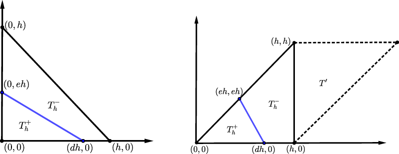
used to construct IFE functions in (3.1). Without loss of generality, in the following analysis, we only consider the interface element configurations in Figure 9 where
 $T^-_h$
is assumed to be triangular. We first recall a norm equivalence result from Lemma 3.6 in [Reference Guo and Lin35].
Interface element configuration. Left: Case 1 and right: Case 2.

Lemma 7. For each interface element with the configuration shown in Figure 9, if
 $|A_1D|\ge\frac{1}{2}|A_1A_2|$
and
 $|A_1E|\ge\frac{1}{2}|A_1A_3|$
(case 1),
 \begin{align}\| \cdot \|_{L^2\left(T^-_h\right)} \simeq \| \cdot \|_{L^2(T)}, \,\,\,\, \text{on} \,\, \mathcal{ND}_h(T),\end{align}
and if
 $|A_1D|\leqslant\frac{1}{2}|A_1A_2|$
or
 $|A_1E|\leqslant\frac{1}{2}|A_1A_3|$
(case 2),
 \begin{align}\| \cdot \|_{L^2(T^+_h)} \simeq \| \cdot \|_{L^2(T)}, \,\,\,\, \text{on} \,\, \mathcal{ND}_h(T).\end{align}
Then we can show the stability of the extension operator
 $\mathcal{C}_T$
in the following.
Lemma 8. For each interface element T, if
 $|A_1D|\ge\frac{1}{2}|A_1A_2|$
and
 $|A_1E|\ge\frac{1}{2}|A_1A_3|$
(Case 1 in Figure 9),
 \begin{align} \| \mathcal{C}_T(\textbf{v}_h) \|_{L^2\left(T^-_h\right)} \lesssim \| \textbf{v}_h \|_{L^2\left(T^-_h\right)}, \,\,\, \text{and} \,\,\, \| \mathcal{C}^{-1}_T(\textbf{v}_h) \|_{L^2\left(T^-_h\right)} \lesssim \| \textbf{v}_h \|_{L^2\left(T^-_h\right)}, \,\,\, \forall \textbf{v}_h\in\mathcal{ND}_h(T);\end{align}
if
 $|A_1D|\leqslant\frac{1}{2}|A_1A_2|$
or
 $|A_1E|\leqslant\frac{1}{2}|A_1A_3|$
(Case 2 in Figure 9),
 \begin{align} \| \mathcal{C}_T(\textbf{v}_h) \|_{L^2(T^+_h)} \lesssim \| \textbf{v}_h \|_{L^2(T^+_h)} \,\,\, \text{and} \,\,\, \| \mathcal{C}^{-1}_T(\textbf{v}_h) \|_{L^2(T^+_h)} \lesssim \| \textbf{v}_h \|_{L^2(T^+_h)}, \,\,\, \forall \textbf{v}_h\in\mathcal{ND}_h(T) .\end{align}
Proof. For simplicity, we only prove the first one in (5.5a). Let
 $D=[x_{D,1},x_{D,2}]^t$
in the explicit formula in (3.2). Note that
 $\text{curl}\,\textbf{v}$
is a constant. Then if
 $|A_1D|\ge\frac{1}{2}|A_1A_2|$
and
 $|A_1E|\ge\frac{1}{2}|A_1A_3|$
, the formula of
 $b_1$
in (3.2) leads to
 \begin{equation}|b_1| \lesssim | \text{curl}\,\textbf{v}_h | \lesssim h^{-1}_T \| \text{curl}\,\textbf{v}_h \|_{L^2(T)} \lesssim h^{-2}_T \| \textbf{v}_h \|_{L^2(T)} \lesssim h^{-2}_T \| \textbf{v}_h \|_{L^2\left(T^-_h\right)},\end{equation}
where in the last two inequalities above we have used the inverse inequality and norm equivalence (5.4a). In addition, we note that there exists a constant C such that
 $|\triangle A_1DE|/|DE|\ge Ch$
where C is independent of interface location. So by the trace inequalities for polynomials [Reference Warburton and Hesthaven64] we have
 $|\textbf{v}_h(X_m)\cdot\bar{\textbf{n}}|\lesssim h^{-1}_T\|\textbf{v}_h \|_{L^2(\triangle A_1DE)} \simeq h^{-1}_T \| \textbf{v}_h \|_{L^2\left(T^-_h\right)}$
. Putting this estimate and (5.6) into the formula of
 $b_2$
in (3.2), we obtain
 \begin{equation}|b_2| \lesssim h^{-1}_T \| \textbf{v}_h \|_{L^2\left(T^-_h\right)} + h_T |b_1| \lesssim h^{-1}_T \| \textbf{v}_h \|_{L^2\left(T^-_h\right)} .\end{equation}
Now using the expression of
 $\mathcal{C}_T(\textbf{v}_h)$
in (3.2), we have
 \begin{equation} \| \mathcal{C}_T(\textbf{v}_h) \|_{L^2\left(T^-_h\right)} \lesssim \| \textbf{v}_h \|_{L^2\left(T^-_h\right)} + h^2_T |b_1| + h_T |b_2| \lesssim \| \textbf{v}_h \|_{L^2\left(T^-_h\right)},\end{equation}
which has finished the proof of the first one in (5.5a). The argument for other estimates is similar.
The stability enables us to prove a trace inequality of the IFE functions.
Theorem 5.2. For each interface element T and its edge e, there holds
 \begin{equation}\| \textbf{z}_h \|_{L^2(e)} \lesssim h^{-1/2}_T \| \textbf{z}_h \|_{L^2(T)}, \,\,\,\,\, \forall \textbf{z}_h\in \mathcal{IND}_h(T).\end{equation}
Proof. Without loss of generality, we only consider the case that
 $|A_1D|\ge\frac{1}{2}|A_1A_2|$
and
 $|A_1E|\ge\frac{1}{2}|A_1A_3|$
as shown by Case 1 in Figure 9. On the interface edge
 $A_1A_2$
, the standard trace inequality [Reference Warburton and Hesthaven64] yields
 \begin{equation}\| \textbf{z}_h \|_{L^2(A_1D)} \lesssim h^{-1/2}_T \| \textbf{z}_h \|_{L^2(\triangle A_1DE)} \,\,\, \text{and} \,\,\, \| \textbf{z}_h \|_{L^2(DA_2)} \lesssim h^{-1/2}_T \| \textbf{z}_h \|_{L^2(\triangle DA_2E)},\end{equation}
since the distance from the point E to
 $A_1A_2$
is bounded below regardless of interface location, which yields the estimate on this edge. The argument for the interface edge
 $A_1A_3$
is similar. For the non-interface edge
 $A_2A_3$
, by the standard trace inequality and (5.5a), we obtain
 \begin{equation}\begin{split}\| \textbf{z}_h^+ \|_{L^2(A_2A_3)} & \lesssim h^{-1/2}_T \| \textbf{z}^+_h \|_{L^2(T)} = h^{-1/2}_T ( \| \mathcal{C}^{-1}_T(\textbf{z}^-_h) \|_{L^2\left(T^-_h\right)} + \| \textbf{z}^+_h \|_{L^2(T^+_h)} ) \\& \lesssim h^{-1/2}_T ( \| \textbf{z}^-_h \|_{L^2\left(T^-_h\right)} + \| \textbf{z}^+_h \|_{L^2(T^+_h)} ) ,\end{split}\end{equation}
which yields the desired result. The argument for the Case 2 in Figure 9 is similar and relies on (5.5b).
Now, with the trace inequality, we are able to show the stability of the isomorphism
 $\mathbb{\Pi}_h$
.
Theorem 5.3. These exist constants
 $c_2$
and
 $C_2$
independent of interface location such that, on each element T,
 \begin{align} & c_2 \| \textbf{z}_h \|_{L^2(T)} \leqslant \| \mathbb{\Pi}_{h} \textbf{z}_h \|_{L^2(T)} \leqslant C_2 \| \textbf{z}_h \|_{L^2(T)} \,\,\, \forall \textbf{z}_h\in\mathcal{IND}_h(T), \end{align}
 \begin{align} & c_2 \| \textrm{curl}\,\textbf{z}_h \|_{L^2(T)} \leqslant \| \textrm{curl}\,\mathbb{\Pi}_{h} \textbf{z}_h \|_{L^2(T)} \leqslant C_2 \| \textrm{curl}\,\textbf{z}_h \|_{L^2(T)} \,\,\, \forall \textbf{z}_h\in\mathcal{IND}_h(T). \end{align}
Proof. These inequalities for non-interface elements are trivial, and we only consider the interface elements here. For (5.12a), using the argument similar to (4.22) with (3.6a), we obtain
 \begin{equation}\|{\mathbb{\Pi}_{h}\textbf{z}_h}\|_{L^2(T)} = \bigg\|{\sum_{i=1}^3 \int_{e_i} \textbf{z}_h\cdot\textbf{t}_i ds \boldsymbol{\psi}_i}\bigg\|_{L^2(T)}\lesssim \sum_{i=1}^3 h^{1/2}_T \| \textbf{z}_h \|_{L^2(e_i)}.\end{equation}
Applying the trace inequality in Theorem 5.2 to (5.13) yields the right inequality of (5.12a). The left one can be obtained by applying this argument to
 $\mathbb{\Pi}^{-1}_{h}$
. In addition, (5.12b) is a direct consequence of the identity in (3.15).
5.2. A special decomposition
We now establish a special discrete regular decomposition. For this purpose, we need a domain decomposition. Recalling that
 $\mathcal{T}^i_h$
is the collection of interface elements, we define
 \begin{equation}\Omega^i_h=\cup_{T\in\mathcal{T}^i_h} T.\end{equation}
Furthermore, we need a region by expanding one more layer of elements from
 $\mathcal{T}^i_h$
:
 \begin{equation}\begin{split}\mathcal{T}^{\Gamma}_h &\,:\!=\, \left\{ T\in \mathcal{T}_h \,:\, \exists T^{\prime}\in \mathcal{T}^{i}_h \, \text{such that}\,\partial T \cap \partial T^{\prime} \neq \emptyset \right\}, \\[4pt]\Omega^{\Gamma}_h &\,:\!=\, \cup_{T\in\mathcal{T}^{\Gamma}_h} T,\,\,\, \text{and} \,\,\,\Omega^{\Gamma,\pm}_h = \Omega^{\Gamma}_h\cap \Omega^{\pm}.\end{split}\end{equation}
To illustrate the regions, here we show
 $\Omega^{\Gamma}_h$
and
 $\mathcal{T}^{\Gamma}_h$
in the middle plot in Figure 10 and show
 $\mathcal{T}^{\Gamma}_h\backslash \mathcal{T}^i_h$
and
 $\Omega^{\Gamma}_h\backslash\Omega^{i}_h$
by the yellow-shaded region in the left plot in Figure 10. Furthermore, we let
 \begin{equation}\gamma = \partial\Omega^{i}_h \cap \Omega^+,\end{equation}
i.e., the part of the boundary of
 $\Omega^{i}_h$
in
 $\Omega^+$
, which is highlighted by the blue polyline in the middle plot in Figure 10. In the following discussion, we shall employ
 $\mathcal{ND}_{h,0}(D)$
,
 $\mathcal{IND}_{h,0}(D)$
,
 $S_{h,0}(D)$
,
 $\widetilde{S}_{h,0}(D)$
as the subspaces with the zero trace on
 $\partial D$
for a subdomain D formed by elements in
 $\mathcal{T}_h$
contained in D.
Left:
 $\mathcal{T}^{\Gamma}_h\backslash \mathcal{T}^i_h$
and
 $\Omega^{\Gamma}_h\backslash\Omega^i_h$
. Middle:
 $\mathcal{T}^{\Gamma}_h$
,
 $\Omega^{\Gamma}_h$
and
 $\gamma$
. Right: a patch near the interface.

Lemma 9.
(A Special Discrete Decomposition) For each
 $\textbf{u}_h\in \mathcal{ND}_{h,0}(\Omega)$
(or
 $\mathcal{IND}_{h,0}(\Omega)$
), there exists a
 $\textbf{u}^{\ast}_h\in\mathcal{ND}_{h,0}(\Omega)$
(or
 $\mathcal{IND}_{h,0}(\Omega)$
) and
 ${\mathop{\textbf{u}}\limits^{\tiny\circ}}_h\in\mathcal{ND}_{h,0}(\Omega)\cap\textrm{Ker(curl)}$
(or
 $\mathcal{IND}_{h,0}(\Omega)\cap\textrm{Ker(curl)}$
) such that
 \begin{equation}\textbf{u}_h = \textbf{u}^{\ast}_h + {\mathop{\textbf{u}}\limits^{\tiny\circ}}_h\end{equation}
satisfying that, for a constant
 $C_3$
independent of interface location and mesh size
 \begin{equation}\| \textbf{u}^{\ast}_h \|_{L^2\left(\Omega^{\Gamma}_h\right)} \leqslant C_3h \| \textrm{curl}\, \textbf{u}_h \|_{L^2(\Omega)}.\end{equation}
Proof. The proof is lengthy, and we decompose it into several steps.
Step 1. We first focus on
 $\textbf{u}_h\in\mathcal{ND}_{h,0}(\Omega)$
. We need to construct a function
 $\textbf{v}_h\in\mathcal{ND}_{h,0}(\Omega^{\Gamma,+}_h\cup\Omega^i_h)\cap\text{Ker(curl)}$
such that its trace on
 $\gamma$
matches
 $\textbf{u}_h$
except one edge denoted by
 $e^{\ast}$
of the polyline
 $\gamma$
in (5.16). Note that
 $\textbf{v}_h$
should have vanishing trace on
 $\partial( \Omega^{\Gamma,+}_h\cup\Omega^i_h)$
, i.e., the two polyline near
 $\gamma$
.
Let us denote the edges on
 $\gamma$
by
 $e_1$
,
 $e_2$
, …,
 $e_N$
with the clockwise orientation with the nodes
 $X_1$
,
 $X_2$
,…,
 $X_N$
. Without loss of generality, we assume
 $e^{\ast}=e_N$
, as shown in the right plot in Figure 10. We consider a linear finite element function
 $v_h$
such that
 $v_h(X_1)=0$
,
 $v_h(X_{n+1})= \sum_{j=1}^{n} \int_{e_j} \textbf{u}_h\cdot\textbf{t} ds$
,
 $n=1,2,...,N-1$
, and it vanishes at all other nodes. Then,
 $v_h\in S_{h,0}(\Omega^{\Gamma,+}_h\cup\Omega^i_h)$
, and
 $\textbf{v}_h=\nabla v_h\in \mathcal{ND}_{h,0}(\Omega^{\Gamma,+}_h\cup\Omega^i_h)$
. Thus, we clearly have
 $\int_{e_n}\textbf{v}_h\cdot\textbf{t} ds = \int_{e_n}\textbf{u}_h\cdot\textbf{t} ds$
,
 $n=1,2,...,N-1$
. Note that
 $\int_{\gamma}\textbf{v}_h\cdot\textbf{t} ds =0$
but
 $\textbf{u}_h$
may not have this property, so
 $\int_{e^{\ast}} \textbf{v}_h\cdot\textbf{t} ds$
may not equal
 $\int_{e^{\ast}} \textbf{u}_h\cdot\textbf{t} ds$
.
Step 2. Let us assume that the closed polyline
 $\gamma$
partitions the whole domain
 $\Omega$
into
 $\Omega_{h,+}$
and
 $\Omega_{h,-}$
where we have
 $\Omega_{h,+}\subseteq\Omega^+$
and
 $\Omega^-\subseteq\Omega_{h,-}$
. Since the triangulation is regular,
 $\gamma$
is a Lipschitz curve, and thus both
 $\Omega_{h,\pm}$
have Lipschitz boundary. Denote
 $\textbf{k}_h = \textbf{u}_h - \textbf{v}_h$
and
 $\textbf{k}^{\pm}_h = (\textbf{u}_h - \textbf{v}_h)|_{\Omega_{h,\pm}}$
. By the discussion in Step 1,
 $\textbf{k}^{+}_h$
has the zero trace on
 $\partial\Omega$
and
 $\gamma\backslash e^{\ast}$
, and
 $\textbf{k}^{-}_h$
simply has the zero trace on
 $\gamma\backslash e^{\ast}$
. Then, we apply the discrete regular decomposition of Theorem 11 in [Reference Hiptmair and Pechstein43] (also see the related discussion in [Reference Hiptmair40, Reference Hiptmair and Pechstein42]) to
 $\textbf{k}^{\pm}_h$
on
 $\Omega_{h,\pm}$
which gives
 \begin{equation*}\textbf{k}^{\pm}_h = \textbf{R}^{\ast}_{\pm} \textbf{z}^{\pm}_h + \textbf{r}^{\pm}_h + \textbf{h}^{\pm}_h, \,\,\,\, \text{on} \, \Omega_{h,\pm},\end{equation*}
where the regular components
 $\textbf{z}^{\pm}_h\in \left[S_{h}(\Omega_{h,\pm})\right]^2$
, the curl-free components
 $\textbf{h}^{\pm}_h\in \mathcal{ND}_{h}(\Omega_{h,\pm})\cap\text{Ker(curl)}$
, the reminders
 $\textbf{r}^{\pm}_h\in\mathcal{ND}_{h}(\Omega_{h,\pm})$
and
 $\textbf{R}^{\ast}_{\pm}\,:\,S_{h}(\Omega_{h,\pm})\rightarrow \mathcal{ND}_{h}(\Omega_{h,\pm})$
are special local projection operators preserving zero boundary conditions. Moreover, these components inherit the zero traces of
 $\textbf{k}^{\pm}_h$
, namely,
 $\textbf{z}^{+}_h$
,
 $\textbf{r}^{+}_h$
and
 $\textbf{h}^{+}_h$
also have the corresponding zero traces on
 $\partial\Omega\cup(\gamma\backslash e^{\ast})$
and the “
 $-$
” components have the zero traces on
 $\gamma\backslash e^{\ast}$
. Furthermore, since
 $e^{\ast}$
is a single edge, the continuity suggests that
 $\textbf{z}^{\pm}_h$
and
 $\textbf{h}^{\pm}_h$
must have the zero traces on the whole
 $\gamma$
. Then we have
 $\textbf{r}^+_h\cdot \textbf{t}=\textbf{k}_h\cdot\textbf{t} = \textbf{r}^-_h\cdot \textbf{t}$
on every edge of
 $\gamma$
. So all these three decomposed components must be tangentially continuous on
 $\gamma$
. Therefore, we can put these components together to define
 $\textbf{z}_h = \textbf{z}^{\pm}_h$
in
 $\Omega_{h,\pm}$
belonging to
 $\left[S_{h,0}(\Omega)\right]^2$
,
 $\textbf{h}_h = \textbf{h}^{\pm}_h$
in
 $\Omega_{h,\pm}$
belonging to
 $\mathcal{ND}_{h,0}(\Omega)\cap\text{Ker(curl)}$
and
 $\textbf{r}_h = \textbf{r}^{\pm}_h$
in
 $\Omega_{h,\pm}$
belonging to
 $\mathcal{ND}_{h,0}(\Omega)$
which satisfy
 \begin{equation}\textbf{u}_h - \textbf{v}_h = \textbf{k}_h = \textbf{R}^{\ast}\textbf{z}_h + \textbf{r}_h + \textbf{h}_h\end{equation}
with
 $\textbf{R}^{\ast} = \textbf{R}^{\ast}_{\pm}$
in
 $\Omega_{h,\pm}$
. By this definition, using the estimates of the components
 $\textbf{z}^{\pm}_h$
,
 $\textbf{h}^{\pm}_h$
and
 $\textbf{r}^{\pm}_h$
in in [Reference Hiptmair and Pechstein43, Theorem 11], and noticing that
 $\textbf{v}_h$
is curl-free, we have
 \begin{align} \| \nabla \textbf{z}_h \|_{L^2(\Omega)} \lesssim \| \text{curl} \, \textbf{u}_h \|_{L^2(\Omega)}, \,\,\| \textbf{r}_h \|_{L^2(\Omega)} \lesssim h \| \text{curl}\, \textbf{u}_h \|_{L^2(\Omega)} \,\,\, \text{and} \,\,\, \| \textbf{h}_h \|_{L^2(\Omega)} \lesssim \| \text{curl}\, \textbf{u}_h \|_{L^2(\Omega)},\end{align}
and for each patch
 $\omega_T$
of an element T, there holds
 \begin{align}&\| \textbf{R}^{\ast} \textbf{z}_h \|_{L^2(T)} \lesssim \| \textbf{z}_h \|_{L^2(\omega_T)} + h_T \| \text{curl}\, \textbf{z}_h \|_{L^2(\omega_T)}.\end{align}
Step 3. We estimate
 $\mathbf{ R}^{\ast}\textbf{z}_h$
on
 $\Omega^{\Gamma}_h$
, i.e., the subdomain given in (5.15). By (5.20b), we obtain
 \begin{equation}\begin{split}\| \textbf{R}^{\ast} \textbf{z}_h \|^2_{L^2\left(\Omega^{\Gamma}_h\right)} &= \sum_{T\in\mathcal{T}^{\Gamma}_h} \| \textbf{R}^{\ast} \textbf{z}_h \|^2_{L^2(T)}\lesssim \sum_{T\in\mathcal{T}^{\Gamma}_h} \left( \| \textbf{z}_h \|_{L^2(\omega_T)} + h_T \| \text{curl}\,\textbf{z}_h \|_{L^2(\omega_T)} \right)^2.\end{split}\end{equation}
For each patch
 $\omega_T$
,
 $T\in\mathcal{T}^{\Gamma}_h$
, without loss of generality we assume
 $T\notin{\mathcal{T}}^i_h$
, i.e., it is not an interface element, and thus there is at least one interface element denoted by T’ such that T’ and T share at least one node denoted by A as shown in the right plot in Figure 10. Since T’ has one node on
 $\gamma$
and
 $\textbf{z}_h$
must vanish at this node, then the estimate of
 $\textbf{z}_h$
on T’ is straightforward through the Poincaré-type inequality:
 \begin{equation}\| \textbf{z}_h \|_{L^2(T^{\prime})} \lesssim h_{T^{\prime}} \| \nabla \textbf{z}_h \|_{L^2(T^{\prime})}.\end{equation}
Then, we also have the estimate for
 $|\textbf{z}_h(A)|$
through the trace inequality and (5.22)
 \begin{equation}| \textbf{z}_h(A) | \lesssim h^{-1}_{T^{\prime}}\| \textbf{z}_h \|_{L^2(T^{\prime})} \lesssim \| \nabla \textbf{z}_h \|_{L^2(T^{\prime})}.\end{equation}
In addition, on T we can write
 $\textbf{z}_h$
as
 $\textbf{z}_h(X)=\textbf{z}_h(A) + \nabla\textbf{z}_h(X-A)$
where
 $\nabla\textbf{z}_h$
is a 2-by-2 constant matrix. Thus (5.23) together with the continuity at A leads to
 \begin{equation}\| \textbf{z}_h \|_{L^2(T)} \lesssim h_T (|\textbf{z}_h(A)| + \| \nabla \textbf{z}_h \|_{L^2(T)} ) \lesssim h_T \| \nabla \textbf{z}_h \|_{L^2(T^{\prime}\cup T)} \lesssim h \| \nabla\textbf{z}_h \|_{L^2(\omega_T)} .\end{equation}
Furthermore, we note that any element T” in
 $\omega_T$
must share at least one node with T denoted by B as shown in the right plot in Figure 10 for an example. Then the similar argument to (5.23) and (5.24) gives the estimate for
 $\| \textbf{z}_h \|_{L^2(T^{\prime\prime})}$
. The results above give the estimate of
 $\textbf{z}_h$
on
 $\omega_T$
. Applying it to (5.21) and using the finite overlapping property together with the first estimate in (5.20a), we obtain
 \begin{equation}\begin{split}\| \textbf{R}^{\ast} \textbf{z}_h \|_{L^2\left(\Omega^{\Gamma}_h\right)} \lesssim \sum_{T\in\mathcal{T}^{\Gamma}_h} h\left( \| \nabla \textbf{z}_h \|_{L^2(\omega_T)} + \| \text{curl}\,\textbf{z}_h \|_{L^2(\omega_T)} \right) \lesssim h \| \text{curl}\,\textbf{z}_h \|_{L^2(\Omega)}.\end{split}\end{equation}
Therefore, by (5.25) and the second estimate in (5.20a), setting
 $\textbf{u}^{\ast}_h = \mathbf{ R}^{\ast}_h\textbf{z}_h + \textbf{r}_h$
and
 ${\mathop{\textbf{u}}\limits^{\tiny\circ}}_h=\textbf{v}_h + \textbf{h}_h$
fulfills the decomposition (5.17) and (5.18) for the case
 $\textbf{u}_h\in\mathcal{ND}_{h,0}(\Omega)$
.
Step 4. Finally, if
 $\textbf{u}_h\in\mathcal{IND}_{h,0}(\Omega)$
, we have
 $\mathbb{\Pi}_h\textbf{u}_h\in\mathcal{ND}_{h,0}(\Omega)$
, and then the previous analysis shows the existence of functions
 $\textbf{w}^{\ast}_h \in\mathcal{ND}_{h,0}(\Omega)$
and
 ${\mathop{\textbf{w}}\limits^{\tiny\circ}}_h\in\mathcal{ND}_{h,0}(\Omega)\cap\text{Ker(curl)}$
such that
 $\mathbb{\Pi}_h\textbf{u}_h= \textbf{w}^{\ast}_h + {\mathop{\textbf{w}}\limits^{\tiny\circ}}_h$
. So we obtain
 $\textbf{u}_h = \textbf{u}^{\ast}_h + {\mathop{\textbf{u}}\limits^{\tiny\circ}}_h$
with
 $\textbf{u}^{\ast}_h = \mathbb{\Pi}^{-1}_h\textbf{w}^{\ast}_h$
and
 ${\mathop{\textbf{u}}\limits^{\tiny\circ}}_h = \mathbb{\Pi}^{-1}_h{\mathop{\textbf{w}}\limits^{\tiny\circ}}_h$
. Here,
 $\textbf{u}^{\ast}_h$
satisfies (5.18) thanks to Theorem 5.3 and
 ${\mathop{\textbf{u}}\limits^{\tiny\circ}}_h\in\mathcal{IND}_{h,0}(\Omega)$
thanks to the curl-free-preserving property of the isomorphism in Theorem 3.4.
5.3. The inf-sup stability
We now combine the estimates above to show the inf-sup stability. The first theorem is to handle the curl term, and it suggests that the stiffness matrix of the PG-IFE method is actually the same as the standard IFE method which uses the IFE functions as the test functions.
Theorem 5.4. On each element T, there holds
 \begin{equation}\int_T \mu^{-1} \text{curl}\,\textbf{z}_h\,\textrm{curl}\,\mathbb{\Pi}_{h}\textbf{z}_h dX = \int_T\mu^{-1} \textrm{curl}\,\textbf{z}_h\,\textrm{curl}\,\textbf{z}_h dX, \,\,\,\,\,\, \forall \textbf{z}_h\in\mathcal{IND}_h(T).\end{equation}
Proof. It is trivial on non-interface elements. On an interface element, we note that
 $\mu^{-1}\text{curl}\,\textbf{z}_h$
is a constant, and then the integration by part yields
 \begin{equation}\begin{split} \mu^{-1}\text{curl}\,\textbf{z}_h \int_{\partial T} \mathbb{\Pi}_{h}\textbf{z}_h\cdot\textbf{t} \, ds = \mu^{-1}\text{curl}\, \textbf{z}_h \int_{\partial T} \textbf{z}_h\cdot\textbf{t} \, ds = \int_T \mu^{-1} \text{curl}\,\textbf{z}_h\,\text{curl}\,\textbf{z}_h dX,\end{split}\end{equation}
where we have also used the continuous tangential jump condition (3.1a).
The next step is to establish an inf-sup stability specially for the curl-free subspaces near the interface elements.
Lemma 10. For the Cartesian mesh, assume the contrast of the conductivity satisfies
 $\max\{\beta^+/\beta^-,$
 $\beta^-/\beta^+\}< 10.65$
, then there holds, for a constant
 $C_4$
independent of interface location and mesh size,
 \begin{equation}(\beta \textbf{u}_h,\mathbb{\Pi}_h\textbf{u}_h)_{L^2\left(\Omega^{\Gamma}_h\right)} \ge C_4\| \textbf{u}_h \|^2_{L^2\left(\Omega^{\Gamma}_h\right)}, \,\,\,\, \forall \textbf{u}_h \in \mathcal{IND}_{h,0}(\Omega)\cap\textrm{Ker(curl)}.\end{equation}
Proof. The argument is technical based on direct calculation, so we put it in Appendix B.
Now we are ready to show the inf-sup condition in (5.1).
Theorem 5.5. Under the conditions of Lemma 10 and for h sufficiently small, the inf-sup condition (5.1) holds regardless of the mesh size and interface location relative to the mesh.
Proof. First of all, Theorem 5.4 directly yields
 \begin{equation}(\mu^{-1} \,\text{curl}\,\textbf{u}_h, \text{curl}\,\mathbb{\Pi}_h\textbf{u}_h)_{L^2(\Omega)} = (\mu^{-1} \,\text{curl}\,\textbf{u}_h, \text{curl}\,\textbf{u}_h)_{L^2(\Omega)} \ge 1/\min\{\mu^-,\mu^+\} \| \text{curl}\,\textbf{u}_h \|^2_{L^2(\Omega)}.\end{equation}
Since
 $\mathbb{\Pi}_h\textbf{u}_h=\textbf{u}_h$
on
 $\Omega\backslash\Omega^{\Gamma}_h$
, we certainly have
 \begin{equation}(\beta\, \textbf{u}_h, \mathbb{\Pi}_h\textbf{u}_h)_{L^2\left(\Omega\backslash\Omega^{\Gamma}_h\right)} \ge \min\{\beta^-,\beta^+\} \| \textbf{u}_h \|^2_{L^2\left(\Omega\backslash\Omega^{\Gamma}_h\right)}.\end{equation}
As for
 $\Omega^{\Gamma}_h$
, applying the decomposition in Lemma 9, the estimate in Lemma 10 and the stability in Theorem 5.3 together with the arithmetic inequality, for h sufficiently small we have
 \begin{equation}\begin{split}& (\beta\,(\textbf{u}^{\ast}_h+{\mathop{\textbf{u}}\limits^{\tiny\circ}}_h), \mathbb{\Pi}_h(\textbf{u}^{\ast}_h+{\mathop{\textbf{u}}\limits^{\tiny\circ}}_h))_{L^2\left(\Omega^{\Gamma}_h\right)} \\& \quad = (\beta \textbf{u}^{\ast}_h, \textbf{u}^{\ast}_h)_{L^2\left(\Omega^{\Gamma}_h\right)} + (\beta\,{\mathop{\textbf{u}}\limits^{\tiny\circ}}_h, \mathbb{\Pi}_h{\mathop{\textbf{u}}\limits^{\tiny\circ}}_h)_{L^2\left(\Omega^{\Gamma}_h\right)} \\& \qquad + (\beta \textbf{u}^{\ast}_h, \mathbb{\Pi}_h\textbf{u}^{\ast}_h - \textbf{u}^{\ast}_h)_{L^2\left(\Omega^{\Gamma}_h\right)} + (\beta\,\textbf{u}^{\ast}_h, \mathbb{\Pi}_h{\mathop{\textbf{u}}\limits^{\tiny\circ}}_h)_{L^2\left(\Omega^{\Gamma}_h\right)} + (\beta\,{\mathop{\textbf{u}}\limits^{\tiny\circ}}_h, \mathbb{\Pi}_h\textbf{u}^{\ast}_h)_{L^2\left(\Omega^{\Gamma}_h\right)} \\& \quad \ge \min\{\beta^-,\beta^+\} \| \textbf{u}^{\ast}_h \|^2_{L^2\left(\Omega^{\Gamma}_h\right)} + C_4 \| {\mathop{\textbf{u}}\limits^{\tiny\circ}}_h \|^2_{L^2\left(\Omega^{\Gamma}_h\right)} \\ & \qquad - \max\{\beta^-,\beta^+\}\left( 2C^2_3C_2 h^2 \| \text{curl}\, \textbf{u}_h \|^2_{L^2(\Omega)} + C_2C_3 h \| \text{curl}\, \textbf{u}_h \|^2_{L^2(\Omega)} + C_2C_3 h\| {\mathop{\textbf{u}}\limits^{\tiny\circ}}_h \|^2_{L^2\left(\Omega^{\Gamma}_h\right)}\right) \\ & \quad \ge \min\{\beta^-,\beta^+\} \| \textbf{u}^{\ast}_h \|^2_{L^2\left(\Omega^{\Gamma}_h\right)} + (C_4 - hC_2C_3\max\{\beta^-,\beta^+\} ) \| {\mathop{\textbf{u}}\limits^{\tiny\circ}}_h \|^2_{L^2\left(\Omega^{\Gamma}_h\right)} \\ &\qquad - \max\{\beta^-,\beta^+\}C_2C_3 (2C_3h+1) h \| \text{curl}\, \textbf{u}_h \|^2_{L^2(\Omega)} \\ & \quad \ge \min\{\beta^-,\beta^+,C_4\}/2 \| \textbf{u}_h \|^2_{L^2\left(\Omega^{\Gamma}_h\right)} - \max\{\beta^-,\beta^+\}C_2C_3 (2C_3h+1) h \| \text{curl}\, \textbf{u}_h \|^2_{L^2(\Omega)} ,\end{split}\end{equation}
where
 $C_2$
,
 $C_3$
and
 $C_4$
inherit from Theorem 5.3, Lemmas 9 and 10, respectively. Let
 $C_5= \max\{\beta^-,\beta^+\}$
 $C_2C_3 (2C_3h+1)$
. Noticing that
 ${\mathop{\textbf{u}}\limits^{\tiny\circ}}_h$
is curl-free, we finally obtain from Theorem 5.4 and (5.29)–(5.31) that
 \begin{equation}\begin{split}a_h(\textbf{u}_h,\mathbb{\Pi}_h\textbf{u}_h) & = (\mu\,\text{curl}\,\textbf{u}_h, \text{curl}\,\mathbb{\Pi}_h\textbf{u}_h)_{L^2(\Omega)} + (\beta\,\textbf{u}_h, \mathbb{\Pi}_h \textbf{u}_h)_{L^2\left(\Omega\backslash\Omega^{\Gamma}_h\right)} + (\beta\,\textbf{u}_h, \mathbb{\Pi}_h \textbf{u}_h)_{L^2\left(\Omega^{\Gamma}_h\right)} \\& \ge ( 1/\min\{\mu^-,\mu^+\}- C_5 h) \| \text{curl}\, \textbf{u}_h \|^2_{L^2(\Omega)} \\& \quad + \min\{\beta^-,\beta^+,C_4\}/2 \| \textbf{u}_h \|^2_{L^2\left(\Omega^{\Gamma}_h\right)} + \min\{\beta^-,\beta^+\} \| \textbf{u}_h \|^2_{L^2\left(\Omega\backslash\Omega^{\Gamma}_h\right)} \ge C_s \| \textbf{u}_h \|^2_{\textbf{H}(\text{curl};\,\Omega)},\end{split}\end{equation}
which yields the desired result for h sufficiently small.
Remark 5.1. (Comments on the analysis of the inf-sup stability.) If
 $\beta^-=\beta^+$
, Remark 3.4 indicates the curl-free subspaces of FE and IFE spaces are identical. So we have a Poincaré-type inequality:
 \begin{equation}\| \textbf{u}_h - \mathbb{\Pi}_h\textbf{u}_h \|_{L^2(T)} \lesssim h_T \| \textrm{curl}\, \textbf{u}_h \|_{L^2(T)}, \,\,\, \textbf{u}_h\in\mathcal{IND}_h(T).\end{equation}
Then the analysis of the inf-sup stability is straightforward by using (5.33) to estimate the term
 $(\beta\textbf{u}_h,\mathbb{\Pi}_h\textbf{u}_h)_{L^2(\Omega)}$
. However, the estimate (5.33) is only true for continuous conductivity. In fact,
 $\mathcal{IND}_h(T)$
cannot recover the local spaces of constant vectors when the conductivity is discontinuous.
By inspecting the proof of Theorem 5.5, one critical ingredient is the inf-sup stability on the curl-free subspace, i.e., Lemma 10. In this lemma, the Cartesian-mesh assumption is for relatively easy calculation, and we expect that some other bounds can be also obtained for various-shaped elements through a similar derivation, but we note that the critical upper bound value should depend on the mesh geometry. In fact, from (B.4) and the related calculation, the constant
 $C_4$
in Lemma 10 can be specified as
 $C_4 = C^{\prime}_4(10.65- \max\{\beta^-/\beta^+,\beta^+/\beta^-\})$
where
 $C^{\prime}_4$
is independent of the mesh size, interface location and parameters. So
 $C_4$
may be close to 0 if the contrast of
 $\beta$
gets close to this critical upper bound, which causes the loss of coercivity. Indeed, numerical results suggest that
 $(\beta\textbf{u}_h,\mathbb{\Pi}_h\textbf{u}_h)_{L^2(\Omega)}$
fails to satisfy the inf-sup condition when the contrast is beyond this bound.
Nevertheless, in numerical experiments, we have not observed any instability issue for large contrast of conductivity. So for analysis,
 $\mathbb{\Pi}_h$
may not be a suitable operator to generate the test function, and some more appropriate test functions are demanded. Due to the exact sequence in Theorem 3.5, this is highly related to the inf-sup stability for the PG-IFE method for the
 $H^1$
-elliptic interface problems [Reference Hou, Song, Wang and Zhao44] which remains open for years. Lemma 10 gives the estimate under some conditions.
Furthermore, we note that the condition of h being sufficiently small seems to be rather essential not just for analysis, as the matrix
 $\mathbf{ A}+\mathbf{ A}^t$
may have negative eigenvalues on coarse meshes for certain interface shape where
 $\mathbf{ A}$
is the resulting matrix given by (5.34). But again, this does not mean the original inf-sup condition needs the requirement of fine meshes, as a more appropriate test function may be chosen, see the discussion above.
5.4. Condition number estimation
Thanks to the isomorphism
 $\mathbb{\Pi}_{h}$
, the estimation of the condition number for the proposed method becomes quite straightforward. In fact, our analysis reveals that its robustness with respect to small-cut elements essentially relies on the stability of the isomorphism in Theorem 5.3. Let us denote the resulting linear system as
 \begin{equation}{\textbf{A}} \bar{\textbf{u}} = \bar{\textbf{f}},\end{equation}
where A is not symmetric due to the PG formulation unless
 $\mu^+=\mu^-$
and
 $\beta^+=\beta^-$
.
We first recall some estimates for standard Nédélec functions. For each
 $\textbf{v}_h\in \mathcal{ND}_{h,0}(\Omega)$
or
 $\mathcal{IND}_{h,0}(\Omega)$
, we define
 $\mathfrak{I}\textbf{v}_h$
as the coefficients of the global shape functions associated with each edge. Then, there holds that
 \begin{align} & m_1 \| \mathfrak{I}\textbf{v}_h \|_2 \leqslant \| \textbf{v}_h \|_{L^2(\Omega)} \leqslant M_1 \| \mathfrak{I}\textbf{v}_h \|_2, \,\,\, \forall \textbf{v}_h\in \mathcal{ND}_{h,0}(\Omega),\\[-8pt]\nonumber \end{align}
 \begin{align} & m_2 \| \textbf{v}_h \|_{L^2(\Omega)} \leqslant \| \textbf{v}_h \|_{\textbf{H}(\text{curl};\,\Omega)} \leqslant h^{-1} M_2 \| \textbf{v}_h \|_{L^2(\Omega)}, \,\,\, \forall \textbf{v}_h\in \mathcal{ND}_{h,0}(\Omega),\end{align}
where
 $m_i$
and
 $M_i$
,
 $i=1,2$
, only depend on the shape regularity. Then, the isomorphism
 $\mathbb{\Pi}_{h}$
with Theorem 5.3 immediately shows that these results should be also true for the IFE functions:
 \begin{align} & m_1 C^{-1}_2c_2\| \mathfrak{I}\textbf{v}_h \|_2 \leqslant \| \textbf{v}_h \|_{L^2(\Omega)} \leqslant M_1 c^{-1}_2C_2 \| \mathfrak{I}\textbf{v}_h \|_2, \,\,\, \forall \textbf{v}_h\in \mathcal{IND}_{h,0}(\Omega), \\[-8pt]\nonumber \end{align}
 \begin{align} & m_2 C^{-2}_2c^2_2 \| \textbf{v}_h \|_{L^2(\Omega)} \leqslant \| \textbf{v}_h \|_{\textbf{H}(\text{curl};\,\Omega)} \leqslant h^{-1} M_2 c^{-2}_2C^2_2 \| \textbf{v}_h \|_{L^2(\Omega)}, \,\,\, \forall \textbf{v}_h\in \mathcal{IND}_{h,0}(\Omega).\end{align}
where
 $c_2$
and
 $C_2$
are the constants from Theorem 5.3.
Lemma 11. Let
 $\kappa_2({\cdot})$
be the spectral condition number of a matrix. Then
 $\kappa_2({\textbf{A}})\lesssim h^{-2}$
.
Proof. Based on (5.1) and (5.3), we use (5.35b) and (5.36b) to obtain
 \begin{equation} \inf_{\textbf{u}_h\in\mathcal{IND}_{h,0}(\Omega)} \sup_{\textbf{v}_h\in\mathcal{ND}_{h,0}(\Omega)} \frac{a(\textbf{u}_h,\textbf{v}_h)}{ \| \textbf{u}_h \|_{L^2(\Omega)} \| \textbf{v}_h \|_{L^2(\Omega)}} \ge C_s m^2_2 C^{-2}_2 c^2_2, a(\textbf{u}_h,\textbf{v}_h) \leqslant C_1 M^2_2 c^{-2}_2C^2_2 h^{-2} \| \textbf{u}_h \|_{L^2(\Omega)} \| \textbf{v}_h \|_{L^2(\Omega)}. \end{equation}
Then, applying Theorem 3.1 in [Reference Ern and Guermond30] together with (5.35a) and (5.36a), we arrive at
 \begin{equation}\kappa_2({\textbf{A}}) \leqslant \left( C_1M^2_1 M^2_2 C^5_2 \right) \left(C_s m^2_1 m^2_2 c^5_2 \right)^{-1} h^{-2}.\end{equation}
Remarkably, the constant in (5.38) only depends on parameters
 $\mu$
,
 $\beta$
and the shape regularity of the mesh.
6. Numerical examples
In this section, we present a group of numerical experiments to validate the previous analysis. We also compare the numerical performance of the proposed PG-IFE method with a classic IFE (C-IFE) method and a penalty-type IFE method, referred to as the partially penalised IFE method (PP-IFE) method in the literature. The latter two use the Galerkin formulation, namely the IFE functions are used as both the trial functions and test functions. More specifically, they are to find
 $\textbf{u}_h\in \mathcal{IND}_h(\Omega)$
such that
 \begin{equation}a^{(i)}_h(\textbf{u}_h,\textbf{v}_h) = \int_{\Omega} \textbf{f}\cdot\textbf{v}_h dX \,\,\,\, \forall \textbf{v}_h \in \mathcal{IND}_h(\Omega),\end{equation}
where
 $i=1,2$
and the bilinear form for the PP-IFE method is given by
 \begin{equation}\begin{split}a^{(1)}_h(\textbf{u}_h,\textbf{v}_h) &= \int_{\Omega}\mu^{-1}\text{curl}\,\textbf{u}_h\cdot\text{curl}\,\textbf{v}_h dX + \int_{\Omega} \beta \textbf{u}_h\cdot\textbf{v}_h dX - \int_{\mathcal{E}^i_h} \{\mu^{-1}\text{curl}\,\textbf{u}_h\}_e[\textbf{v}_h\cdot\textbf{t}]_e ds \\&- \int_{\mathcal{E}^i_h} \{\mu^{-1}\text{curl}\,\textbf{v}_h\}_e[\textbf{u}_h\cdot\textbf{t}]_e ds + \frac{c_0\max\{\beta^-,\beta^+\}}{h^r} \int_{\mathcal{E}^i_h} [\textbf{u}_h\cdot\textbf{t}]_e \cdot [\textbf{v}_h\cdot\textbf{t}]_e ds,\end{split}\end{equation}
in which
 $\mathcal{E}^i_h$
denotes the collection of interface edges,
 $c_0$
is a positive constant parameter independent of the mesh size, r is a real number parameter,
 $[\textbf{w}_h\cdot\textbf{t}]_e=\textbf{w}_h|_{T_1}\cdot\textbf{t}-\textbf{w}_h|_{T_2}\cdot\textbf{t}$
, and
 $\{\mu^{-1}\text{curl}\,\textbf{w}_h\}_e= \frac{1}{2}\left(\mu^{-1}\text{curl}\,\textbf{w}_h|_{T_1} + \mu^{-1}\text{curl}\,\textbf{w}_h|_{T_2} \right)$
, and the bilinear form for the classic IFE method is
 \begin{equation}a^{(2)}_h(\textbf{u}_h,\textbf{v}_h) = \int_{\Omega}\mu^{-1}\text{curl}\,\textbf{u}_h\cdot\text{curl}\,\textbf{v}_h dX + \int_{\Omega} \beta \textbf{u}_h\cdot\textbf{v}_h dX.\end{equation}
The penalty-type unfitted mesh methods can generally produce optimally convergent solutions for many interface problems, but not for the
 $\textbf{H}(\text{curl})$
problem. See the numerical results below for the IFE method and [Reference Casagrande, Hiptmair and Ostrowski19, Reference Casagrande, Winkelmann, Hiptmair and Ostrowski20] for the Nitsche’s penalty methods.
We consider a domain
 $\Omega=({-}1,1)\times({-}1,1)$
which is partitioned into
 $N\times N$
squares and each square is then cut into two triangles along the diagonal, i.e., the triangular Cartesian mesh shown in the right plot in Figure 10. Our first example is borrowed from [Reference Hiptmair, Li and Zou41]. We consider a circular interface
 $\Gamma\,:\,x^2+y^2=r^2_1$
that cuts
 $\Omega$
into the inside subdomain
 $\Omega^-$
and the outside one
 $\Omega^+$
. On
 $\Omega$
the exact solution is given by
 \begin{equation}\textbf{u} =\begin{cases} & \left(\begin{array}{c} \mu^-\left( - k_1(r_1^2 - x^2 -y^2)y \right) \\[5pt] \mu^-\left( -k_1(r_1^2 - x^2 -y^2)x \right) \end{array}\right) \,\,\,\, \text{in}\, \Omega^-, \\[20pt] & \left(\begin{array}{c} \mu^+\left( - k_2(r_2^2-x^2-y^2)(r_1^2-x^2-y^2)y \right) \\[5pt] \mu^+\left( - k_2(r_2^2-x^2-y^2)(r_1^2-x^2-y^2)x \right) \end{array}\right) \,\,\,\, \text{in}\, \Omega^+,\end{cases}\end{equation}
for which the boundary conditions and the right hand side
 $\textbf{f}$
are calculated accordingly, and
 $k_2=20$
,
 $k_1=k_2(r_2^2-r_1^2)$
with
 $r_1=\pi/5$
and
 $r_2=1$
. We focus the numerical experiments on four groups of parameters: fixing
 $\mu^-=\beta^-=1$
and varying
 $\mu^+=1/10$
or
 $1/100$
and
 $\beta^+=10$
or 100. Here, we emphasise that the analysis is though only for small contrast of conductivity (less than 10.56), there is no issue in computation for larger contrast. Moreover, we choose the stability parameters in (6.2) to be
 $c_0=10$
and
 $r=1$
, and other choices such as
 $c_0=-10,0,100$
and
 $r=-1,-1/2,0,1/2,1$
can give similar suboptimal results. Furthermore, we let
 $e_0=\| \textbf{u} - \textbf{u}_h \|_{\textbf{H}(\text{curl};\,\Omega)}$
, and in order to study the convergence behaviour around the interface, we also define the error
 \begin{equation}e_1 = |\Omega^i_h|^{-1/2}\| \textbf{u} - \textbf{u}_h \|_{\textbf{H}(\text{curl};\,\Omega^i_h)},\end{equation}
where
 $\Omega^i_h$
is given by (5.14). A similar indicator was also used in [Reference Li, Melenk, Wohlmuth and Zou52] to study the error near the interface for the
 $H^1$
-elliptic interface problems.
The results for the error
 $e_0$
are presented in Figure 11 where the convergence behaviour of PG-IFE, PP-IFE and C-IFE methods are indicated by black, red and blue curves, respectively. In addition, there are three dashed lines with the corresponding colour indicating the expected convergence rate
 $\mathcal{O}(h)$
for the PG-IFE method and the approximate rate
 $\mathcal{O}(h^{1/2})$
for the PP-IFE and C-IFE methods. The black error curve almost overlaps with the corresponding dashed line for the PG-IFE method, namely its convergence rate is certainly optimal. However, for the PP-IFE and C-IFE methods, the errors asymptotically have the suboptimal
 $\mathcal{O}(h^{1/2})$
convergence rates. Moreover, as the contrast of
 $\beta$
becomes larger, the advantages of the PG-IFE method over the other two are more evident.
The convergence rates for the errors
 $e_0$
of PG-IFE, PPIFE and C-IFE methods. From left to right:
 $(\mu^+,\beta^+)=(0.1,10)$
,
 $(0.1,100)$
,
 $(0.01,10)$
,
 $(0.01,100)$
.

It is worthwhile to point out that straightforwardly applying the argument of Theorem 2 in [Reference Casagrande, Hiptmair and Ostrowski19] actually suggests that the PP-IFE method should not converge at all near the interface. So we expect the loss of
 $\mathcal{O}(h^{1/2})$
may be due to the pollution of the error near the interface over the whole domain. To further study this issue, we compute and plot the error
 $e_1$
defined in (6.5) for PG-IFE, PP-IFE and C-IFE methods in Figure 12. Still, the black dashed line indicates the expected optimal
 $\mathcal{O}(h)$
convergence rate for the PG-IFE method which matches the true error curve quite well. So the method has optimal accuracy even near the interface. But the numerical results clearly suggest that both the PP-IFE and the C-IFE methods completely fail to converge near the interface. From the numerical experiments here and in [Reference Casagrande, Hiptmair and Ostrowski19], we actually think this issue seems to be very difficult to overcome for penalty-type methods for the proposed method. We believe it clearly shows advantages for the proposed PG formulation.
The convergence rates for the errors
 $e_1$
of PG-IFE, PPIFE and C-IFE methods. From left to right:
 $(\mu^+,\beta^+)=(0.1,10)$
,
 $(0.1,100)$
,
 $(0.01,10)$
,
 $(0.01,100)$
.

In the second example, we consider more complex interface geometry that has a star shape, shown in the left plot in Figure 13. The interface has a level-set function:
 $f(x,y)=\left(x_1^2+x_2^2\right)^2(1+0.6\sin(5\theta(x_1,x_2))-0.2$
, where
 $\theta(x_1,x_2)$
is the angle of the point
 $[x_1,x_2]^t$
. We consider the exact solution
 $\textbf{u}(x_1,x_2)= (\beta^{\pm})^{-1} \nabla f(x_1,x_2)$
in
 $\Omega^{\pm}$
. The errors of numerical solutions are presented in the right plot in Figure 13 which clearly indicate the optimal convergence rate.
Left: a star-shaped interface. Right: the errors for
 $(\mu^-,\mu^+)=(1,0.01)$
and
 $(\beta^-,\beta^+)=$
 $(1,100), (100,1)$
.

Acknowledgements
The work of the first author was funded by NSF DMS-2012465. The work of the second author was supported in parts by HKSAR grant #15302120 and JRI-CAS Lab of Polyu. The work of the third author was substantially supported by Hong Kong RGC General Research Fund (projects 14306921 and 14306719).
Conflicts of interest
None.
A. Construction of IFE Shape Functions
We present the detailed construction procedure for shape functions in (3.4). Without loss of generality, we consider an element with the vertices
 $A_i$
and edges
 $e_i$
,
 $i=1,2,3$
, with
 $e_1=A_2A_3$
,
 $e_2=A_3A_1$
and
 $e_3=A_1A_2$
, see the left plot in Figure A1, where
 $A_1$
locates at the origin (0,0),
 $A_1A_2$
aligns with the
 $x_1$
axis, and the interface
 $\Gamma$
cuts the edges
 $A_1A_2$
and
 $A_1A_3$
with two points D and E, i.e.,
 $\Gamma^T_h=\overline{DE}$
. Let
 $d=|A_1D|/|A_1A_2|\in(0,1]$
and
 $e=|A_1E|/|A_1A_3|\in(0,1]$
. Consider a reference element
 $\hat{T}$
shown in the right plot in Figure A1 with the vertices
 $\hat{A}_1=(0,0)$
,
 $\hat{A}_2=(1,0)$
,
 $\hat{A}_3=(0,1)$
and the corresponding edges
 $\hat{e}_i$
,
 $i=1,2,3$
with the tangential vectors
 $\hat{\textbf{t}}_i$
. Then the affine mapping is given by
 $F_T=B_T\hat{X}$
with the Jacobian matrix
 $B_T$
. By this set-up, we have
 $\hat{D}=F^{-1}_T(D)=(d,0)$
,
 $\hat{E}=F^{-1}_T(E)=(0,e)$
and
 $\hat{X}_m=[d/2,e/2]^t$
. Moreover, we let
 $\hat{\bar{\textbf{t}}}=[\hat{t}_1,\hat{t}_2]^t$
and
 $\hat{\bar{\textbf{n}}}=[\hat{n}_1,\hat{n}_2]^t$
be the images of
 $\bar{\textbf{t}}$
and
 $\bar{\textbf{n}}$
under
 $F^{-1}_T$
. Here,
 $\hat{\bar{\textbf{t}}}$
is also the tangential vector of
 $\hat{E}\hat{D}$
but
 $\hat{\bar{\textbf{n}}}$
may not be normal to
 $\hat{E}\hat{D}$
anymore, and they all may not be unit vectors due to scaling. We further let
 $\hat{\bar{\textbf{n}}}^{\prime}=[e,d]^t$
be the normal vector to
 $\hat{E}\hat{D}$
. By the Piola transformation [Reference Brezzi and Fortin16], an IFE function
 $\textbf{z}$
can be represented as:
 $\textbf{z}(X)=B_T^{-t}(\hat{\textbf{z}}\circ F^{-1}_T)(X)$
, where
 $\hat{\textbf{z}}$
should satisfy the following jump conditions on the reference element
 \begin{equation}\left[\hat{\textbf{z}}\cdot\hat{\bar{\textbf{t}}}\right]_{\hat{\Gamma}^T_h}=0, \,\,\,\,\, \left[\mu^{-1}\text{curl}\,\hat{\textbf{z}}\right]_{\hat{\Gamma}^T_h}=0, \,\,\,\,\,\, \left[\beta\hat{\textbf{z}}\cdot\hat{\bar{\textbf{n}}}\right]_{\hat{X}_m}=0.\end{equation}
Let
 $\hat{\boldsymbol{\phi}}_i$
be the local basis functions of
 $\mathcal{ND}_h(\hat{T})$
associated with the edge
 $\hat{e}_i$
,
 $i=1,2,3$
. Thus, using the first condition in (A.1) together with (3.4) for
 $i=1$
, we have the following expression for
 $\hat{\textbf{z}}$
:
 \begin{equation}\hat{\textbf{z}}=\begin{cases} \hat{\textbf{z}}^- = v_1\hat{\boldsymbol{\phi}}_1 + c_2 \hat{\boldsymbol{\phi}}_2 + c_3 \hat{\boldsymbol{\phi}}_3, \,\,\,\,\,\,\,\,\,\,\,\,\,\,\,\,\,\,\,\,\,\,\,\,\,\,\,\,\,\,\,\,\,\,\,\, \text{in} \, T^-_h, \\[5pt] \hat{\textbf{z}}^+ = \hat{\textbf{z}}^- + b_{1} [\hat{x}_2, -(\hat{x}_1-d)]^t + b_2 [e,d]^t, \,\,\,\,\,\,\, \text{in} \, T^+_h,\end{cases}\end{equation}
where the vectors
 $[\hat{x}_2, -(\hat{x}_1-d)]^t$
and
 $[e,d]^t$
are orthogonal to
 $\hat{E}\hat{D}$
, and
 $\textbf{c}=[c_2,c_3]^t$
and
 ${\textbf{b}}=[b_1,b_2]^t$
are unknown coefficients to be determined. Using the rest two in (A.1), we can rewrite the following equation for b and
 $\textbf{c}$
 \begin{equation}\mathbf{ A} {\textbf{b}}= \boldsymbol{\gamma} v_1 + \mathbf{ B} \textbf{c}\end{equation}
where
 $\mathbf{ A} = \left[\begin{array}{c@{\quad}c} 1 & 0 \\ \alpha & 2\alpha \end{array}\right], \,\,\,\,\boldsymbol{\gamma} = \left[\begin{array}{c} \kappa \\[3pt] -\lambda\hat{\boldsymbol{\phi}}_1(\hat{X}_m)\cdot\hat{\bar{\textbf{n}}} \end{array}\right], \,\,\,\,\mathbf{ B} = \left[\begin{array}{c@{\quad}c} \kappa & \kappa \\[3pt] -\lambda\hat{\boldsymbol{\phi}}_2(\hat{X}_m)\cdot\hat{\bar{\textbf{n}}} & -\lambda\hat{\boldsymbol{\phi}}_3(\hat{X}_m)\cdot\hat{\bar{\textbf{n}}} \end{array}\right],$
with
 $\alpha=\frac{1}{2}(e\hat{n}_1+d\hat{n}_2)=\frac{1}{2}\hat{\bar{\textbf{n}}}^{\prime}\cdot\hat{\bar{\textbf{n}}}$
,
 $\kappa=1-\frac{\mu^+}{\mu^-}$
and
 $\lambda=1-\frac{\beta^-}{\beta^+}$
. Furthermore, we can use (3.4) for
 $i=2,3$
to obtain
 \begin{equation}\mathbf{ I}_2 \textbf{c} + \mathbf{ R} {\textbf{b}} = \textbf{v},\end{equation}
where
 $\mathbf{ I}_2$
is the
 $2\times2$
identity matrix,
 $\mathbf{ R}=de[{-}1,-1;0,1]$
and
 $\textbf{v}=[v_2,v_3]^t$
. Solving the linear systems (A.3) and (A.4), we can compute all the unknown coefficients in (A.2).
The affine mapping between the physical element and the reference element.

A.1. Proof of Theorem 3.1
Under the notations above, by the assumption that T does not have obtuse angles, we can verify that
 \begin{equation}\hat{\bar{\textbf{n}}}^{\prime}\cdot\hat{\bar{\textbf{n}}} >0 \,\,\, \text{and} \,\,\, \frac{de(\hat{n}_1+\hat{n}_2)}{\hat{\bar{\textbf{n}}}^{\prime}\cdot\hat{\bar{\textbf{n}}}} \in [0,1].\end{equation}
Since the derivation is quite technical and elementary, we postpone it to the end of this subsection. By the first inequality above, we know that
 $\alpha=\frac{1}{2}\hat{\bar{\textbf{n}}}^{\prime}\cdot\hat{\bar{\textbf{n}}}>0$
and thus
 $\mathbf{ A}$
is invertible. So (A.3) gives the formula to compute b in terms of
 $\textbf{c}$
. Putting it into (A.4), we have the following linear system
 \begin{equation}( \mathbf{ I} + \mathbf{ R} \mathbf{ A}^{-1} \mathbf{ B} ) \textbf{c} = \textbf{v} - \mathbf{ A}^{-1} \boldsymbol{\gamma} v_1.\end{equation}
We only need to show the non-singularity of the matrix in
 $\mathbf{ I} + \mathbf{ R} \mathbf{ A}^{-1} \mathbf{ B}$
for the reference element. Direct computation shows that the matrix
 $\mathbf{ I} + \mathbf{ R} \mathbf{ A}^{-1} \mathbf{ B}$
has two eigenvalues
 $1 -de \kappa \,\text{and} \, 1-\frac{de(\hat{n}_1 + \hat{n}_2) \lambda}{ e\hat{n}_1 + d\hat{n}_2 }.$
Because
 $d,e\in[0,1]$
, using the second inequality in (A.5), we have
 \begin{equation*}1 - de \kappa \ge \min\Big\{ 1, \frac{\mu^+}{\mu^-} \Big\}>0 \,\,\, \text{and} \,\,\, 1-\frac{de(\hat{n}_1 + \hat{n}_2) \lambda}{ e\hat{n}_1 + d\hat{n}_2 } \ge \min\Big\{ 1, \frac{\beta^-}{\beta^+} \Big\}>0,\end{equation*}
which finishes the proof.
Now, let us go back to (A.5). First of all, we let
 $l_2=|e_2|$
,
 $l_3=|e_3|$
and
 $\theta=\angle A_3A_1A_2$
as shown by the left plot in Figure A1. Let
 $\delta$
be the angle between the normal vector
 $\bar{\textbf{n}}$
and the
 $x_1$
axis, and it is easy to see
 $\delta\in[\theta-\pi/2,\pi/2]$
. Then we can express
 $B_T$
and
 $\hat{\bar{\textbf{n}}}$
as
 \begin{equation}B_T = \left[\begin{array}{c@{\quad}c} l_3 & l_2\cos(\theta) \\[5pt] 0 & l_2\sin(\theta) \end{array}\right], \,\,\,\, \text{and} \,\,\,\,\hat{\bar{\textbf{n}}} = \frac{1}{l_2l_2 \sin(\theta)} \left[\begin{array}{c} l_2 \sin(\theta-\delta) \\[5pt] l_3\sin(\delta) \end{array}\right].\end{equation}
For the first term in (A.5), by direct calculation, we have
 $2\alpha = \hat{\bar{\textbf{n}}}^{\prime}\cdot\hat{\bar{\textbf{n}}} = \frac{|\Gamma^T_h|}{l_2l_3\sin(\theta)}>0$
. For the second term in (A.5), by direct computation we have.
 \begin{equation*}\hat{n}_1+\hat{n}_2 = \frac{ l_2 \sin(\theta-\delta) + l_3\sin(\delta) }{l_2l_3 \sin(\theta)}= \frac{\cos(\delta)}{\sin(\theta)} \left( \frac{ \sin(\theta) - \cos(\theta)\tan(\delta) }{l_3} + \frac{\tan(\delta)}{l_2} \right),\end{equation*}
 \begin{equation*}e\hat{n}_1 + d\hat{n}_2 - de( \hat{n}_1 + \hat{n}_2 ) = l_2l_3 \cos(\theta) \left( e^2(1-d) \frac{l_2}{l_3\cos(\theta)} + d^2(1-e)\frac{l_3}{l_2\cos(\theta)} - (2de-d^2e-e^2d) \right).\end{equation*}
It can be verified that both these two terms are non-negative since
 $\theta\leqslant \pi/2$
and
 $d,e\in[0,1]$
.
A.2. Proof of Theorem 3.2
We first give the explicit expression of the matrix in (A.6):
 \begin{equation}\mathbf{ I} + \mathbf{ R} \mathbf{ A}^{-1} \mathbf{ B} =\left[\begin{array}{c@{\quad}c}1 + \dfrac{de}{2}\left( -\kappa + \dfrac{\lambda s_2}{\alpha} \right) & \dfrac{de}{2}\left( -\kappa + \dfrac{\lambda s_3}{\alpha} \right) \\[15pt]\dfrac{de}{2}\left( -\kappa - \dfrac{\lambda s_2}{\alpha} \right) & 1 + \dfrac{de}{2}\left( -\kappa - \dfrac{\lambda s_3}{\alpha} \right)\end{array}\right],\end{equation}
where
 $s_2=\hat{\boldsymbol{\phi}}_2(X_m)\cdot\hat{\bar{\textbf{n}}}=-\frac{e}{2}\hat{n}_1 + \left( \frac{d}{2}-1 \right)\hat{n}_2$
and
 $s_3=\hat{\boldsymbol{\phi}}_3(X_m)\cdot\hat{\bar{\textbf{n}}}= \left( 1-\frac{e}{2} \right)\hat{n}_1 + \frac{d}{2} \hat{n}_2$
. Using (A.7),
 $|\Gamma^T_h| \ge \max\{dl_3,el_2\}\sin(\theta)$
and the shape regularity of T and
 $d,e\leqslant1$
, we have
 $\vert{ \frac{de s_2}{\alpha} } \lesssim 1$
and
 $\vert{ \frac{de s_3}{\alpha} } \lesssim 1$
. Therefore, by (A.1) we have
 $\| (\mathbf{ I} + \mathbf{ R} \mathbf{ A}^{-1} \mathbf{ B})^{-1} \|_{\infty} \lesssim 1$
. Furthermore, we note that
 \begin{equation}\mathbf{ A}^{-1}\boldsymbol{\gamma} = \left[\begin{array}{c} \kappa \\[5pt] -\frac{1}{2}(\kappa+ \frac{\lambda}{\alpha}s_1) \end{array}\right],\end{equation}
where
 $s_1=\hat{\boldsymbol{\phi}}_1(X_m)\cdot\hat{\textbf{n}}=(e\hat{n}_1 - d\hat{n}_2)/2$
. Using (A.7), the shape regularity and
 $d,e\leqslant 1$
, we have
 $\vert{\frac{s_1}{\alpha}} \lesssim 1$
, and thus obtain
 $\| \mathbf{ A}^{-1} \boldsymbol{\gamma} \|_{\infty} \lesssim 1$
. Putting the estimates above into the formula (A.6), we have
 $\| \textbf{c} \|_{\infty} \lesssim 1$
. Next, we note that
 \begin{equation}\mathbf{ A}^{-1}\mathbf{ B} =\left[\begin{array}{c@{\quad}c} \kappa & \kappa \\[5pt] \left({-}\kappa - \lambda\dfrac{s_2}{\alpha} \right) & \left({-}\kappa - \lambda\dfrac{s_3}{\alpha} \right) \end{array}\right].\end{equation}
Therefore, putting (A.9) and (A.10) into the formula for b in (A.3), we have
 $|b_1| \lesssim 1$
, and
 $|b_2| \lesssim 1$
where we have used the estimates for
 $s_i/\alpha$
,
 $i=1,2,3$
. Besides, the estimate
 $|\Gamma^T_h|\ge \max\{dl_3,el_2\}\sin(\theta)$
yields
 $|b_2|e, |b_2|d \lesssim 1$
. Finally, the estimates above together with (A.1) yield
 $\| \hat{\textbf{z}} \|_{L^{\infty}(T)} \lesssim 1$
. Hence, the desired result (3.6a) follows from the Piola transformation. At last, (3.6b) can be derived by integration by parts.
B. Proof of Lemma 10
We let
 $\bar{\textbf{n}}=[n_1,n_2]$
and
 $\bar{\textbf{t}}=[{-}n_2,n_1]$
be the normal and tangential vectors to linearly-approximate interface
 $\Gamma^T_h$
. Define a transmission orthogonal matrix
 $\textbf{Q}=[\bar{\textbf{t}},\bar{\textbf{n}}]^t$
and a diagonal matrix
 $\boldsymbol{\Lambda}=\left[\begin{array}{c@{\quad}c} 1 & 0 \\ 0 & \rho \end{array}\right]$
with
 $\rho=\beta^-/\beta^+$
. By the exact sequence for IFE functions, we know
 $\mathcal{IND}_h(T)\cap\text{Ker(curl)}$
consists of piecewise constant vectors on T, and thus, without loss of generality, we assume
 $\textbf{u}_h^-=\textbf{u}_h|_{T^-_h}$
is a constant unit vector. Then we write
 $\textbf{u}^+_h = \textbf{Q}^t\boldsymbol{\Lambda}\textbf{Q}\textbf{u}^-_h$
. So our object is to show
 \begin{equation}(\textbf{u}_h, \mathbb{\Pi}_h\textbf{u}_h)_{D} \ge Ch^2\end{equation}
with some constant C independent of interface location. If D is just each interface element, the desired estimate (B.1) may only hold with a more restrictive bound for
 $\rho$
. Here, we shall include one neighbourhood non-interface element T’, i.e., let
 $D =T\cup T^{\prime}$
for each T, to obtain a better bound for
 $\rho$
.
To avoid redundancy, we only discuss the case that the interface cuts the two adjacent edges of a non-right angle as shown in the right plot in Figure B1. The discussion for the case that the interface cuts the two adjacent edges of the right angle, i.e., the left plot in Figure B1, is similar and actually easier due to symmetry. Without loss of generality, we consider the element of the configuration shown by the right plot in Figure B1, with the vertices
 $A_1=(0,0)$
,
 $A_2=(h,0)$
and
 $A_3=(h,h)$
.
Interface element configuration: Case 1(left) and Case 2(right).

In the following discussion, we shall employ
 $\mathbb{\Pi}_{T}\textbf{u}_h\,:\!=\,\mathbb{\Pi}_{h}\textbf{u}_h|_T$
. We denote the unit normal and tangential vectors to the non-interface edge
 $e_1$
connecting (h,0) and (h,h) by
 $\textbf{n}_1$
and
 $\textbf{t}_1$
, and let
 $\textbf{u}^-_h=a\textbf{n}_1 + b\textbf{t}_1$
with
 $a^2+b^2=1$
. Without loss of generality, we assume
 $a \ge 0$
. Due to the continuity of
 $\textbf{u}_h$
along the tangential direction of the non-interface edge, we have
 $\textbf{u}_h|_{T^{\prime}}=a^{\prime}\textbf{n}_1 + b\textbf{t}_1$
on T’, and then obtain
 $\textbf{u}_h\cdot\mathbb{\Pi}_{T^{\prime}}\textbf{u}_h = a^{\prime 2}+b^2$
on T’. Therefore,
 \begin{equation}\begin{split}(\beta\textbf{u}_h, \mathbb{\Pi}_{T}\textbf{u}_h)_{L^2(T)} + (\beta^-\textbf{u}_h,\mathbb{\Pi}_{T^{\prime}}\textbf{u}_h )_{L^2(T^{\prime})} = \beta^-(\textbf{u}^-_h\cdot\mathbb{\Pi}_{T}\textbf{u}_h + b^2 )|T^-_h| + \beta^+( \textbf{u}^+_h\cdot\mathbb{\Pi}_{T}\textbf{u}_h + \rho b^2 ) |T^+_h| + a^{\prime 2}|T^{\prime}| \end{split}\end{equation}
where we have implicitly used
 $|T^{\prime}|=|T|$
. We shall proceed to estimate each one of the first two terms above.
Let the interface-intersection points be
 $D=(dh,0)$
and
 $E=(eh,eh)$
,
 $d,e\in[0,1]$
. Then, we can express
 $n_1=e/\sqrt{(d-e)^2+e^2}$
and
 $n_2=(d-e)/\sqrt{(d-e)^2+e^2}$
. By the direct calculation, we obtain
 \begin{equation}\begin{split}\mathbb{\Pi}_{T}\textbf{u}_h = \textbf{u}^-_h + \frac{(\rho-1)}{(d-e)^2 + e^2} \left[\begin{array}{c@{\quad}c} de^2 & de(d-e) \\[5pt] 0 & 0 \end{array}\right] \textbf{u}^-_h = (\textbf{I}_2 + (\rho-1) {\textbf{B}}_1)\textbf{u}^-_h,\end{split}\end{equation}
which is a constant vector as
 $\mathbb{\Pi}_{T}\textbf{u}_h\in \nabla S_h(T)$
. Let
 $\alpha_1=\textbf{n}_1^t{\textbf{B}}_1\textbf{n}_1$
and
 $\alpha_2=\textbf{n}_1^t{\textbf{B}}_1\textbf{t}_1$
, and notice
 $\textbf{t}_1^t{\textbf{B}}_1=0$
. Then,
 \begin{equation}\textbf{u}^-_h\cdot\mathbb{\Pi}_{T}\textbf{u}_h = 1 + (\rho-1)\left(a^2\alpha_1 + ab\alpha_2\right).\end{equation}
The direct calculation yields the following estimates
 \begin{equation}\begin{split}& \alpha_1 = \frac{de^2}{(d-e)^2 + e^2} \in [0,1], \,\, \alpha_2 = \frac{de(d-e)}{(d-e)^2 + e^2} \in \left[(1-\sqrt{2})/2,0.5\right]\,\, \text{and} \,\, \alpha_1^2 + \alpha_2^2 \leqslant 1.\end{split}\end{equation}
Then if
 $\rho \leqslant 1$
, using the estimate
 $a^2\alpha_1+ab\alpha_2 \leqslant a\sqrt{a^2+b^2}\sqrt{\alpha_1^2+\alpha_2^2} \leqslant a$
, we have
 \begin{equation}\textbf{u}^-_h|_T\cdot\mathbb{\Pi}_{T}\textbf{u}_{h} \ge 1 - a + \rho a \ge \rho.\end{equation}
It remains to show the estimate for
 $\rho > 1$
. If
 $a^2\alpha_1 + ab\alpha_2\ge 0$
, then
 $\textbf{u}^-_h\cdot\mathbb{\Pi}_T\textbf{u}_h \ge C$
. In addition, if
 $a^2\alpha_1 + ab\alpha_2 < 0$
, the direct calculation yields
 \begin{equation}\frac{-(1+b^2)}{a^2\alpha_1 + ab\alpha_2} \ge 2 \sqrt{2} \sqrt{ \frac{((d^2 - 2 d e + 2 e^2)^2 (d^2 - 2 d e + 3 e^2))}{( d^2 (d - e)^4 e^2)} } + \frac{4((d - e)^2 + e^2)}{d(d - e)^2} \ge 2 (4 + 2 \sqrt{2}).\end{equation}
Hence, the following estimate is true for
 $\rho=\beta^-/\beta^+\in (1,9+4\sqrt{2})$
where
 $9+4\sqrt{2}\approx 14.65$
 \begin{equation}\textbf{u}^-_h\cdot\mathbb{\Pi}_{T}\textbf{u}_h + b^2 \ge 1+ b^2 + (\rho-1)\left(a^2\alpha_1 + ab\alpha_2\right) \ge C.\end{equation}
As for
 $\textbf{u}^+_h$
, the similar derivation yields
 \begin{equation}\textbf{u}^+_h\cdot\mathbb{\Pi}_{T}\textbf{u}_h \ge C \,\,\, \text{if} \, \rho^{-1} \leqslant 1 \,\,\, \text{and} \,\,\, \textbf{u}^+_h\cdot\mathbb{\Pi}_{T}\textbf{u}_h + \rho b^2 \ge C \,\,\, \text{if} \, \rho^{-1} \leqslant 10.655.\end{equation}
Substituting (B.8) and (B.9) into (B.4) yields the desired result.