





Introduction
Thwaites Glacier has been actively retreating in response to sub-shelf melt from enhanced circumpolar deep-water intrusion onto the Antarctic continental shelf (e.g. Pritchard and others, Reference Pritchard, Ligtenberg, Fricker, Vaughan, Van den Broeke and Padman2012; Joughin and others, Reference Joughin, Smith and Medley2014; Mouginot and others, Reference Mouginot, Rignot and Scheuchl2014; Rignot and others, Reference Rignot, Mouginot, Morlighem, Seroussi and Scheuchl2014; Sutterley and others, Reference Sutterley2014). This incursion trend is expected to continue and, as past warmer periods have produced rapid retreat on Thwaites (Graham and others, Reference Graham2022), it is likely that continued sub-shelf melt will maintain or accelerate mass loss and associated sea-level rise. Given its unique position as a climatic tipping point situated in the ‘weak underbelly’ (Hughes, Reference Hughes1981) of the West Antarctic Ice Sheet (WAIS), it is critical to reduce uncertainty in estimates of Thwaites’ potential timelines of retreat.
Predictive models seeking to anticipate sea-level contributions from the Amundsen Sea Embayment (ASE) sector of the WAIS tend to diverge (e.g. Yu and others, Reference Yu, Rignot, Seroussi and Morlighem2018; Hoffman and others, Reference Hoffman, Asay-Davis, Price, Fyk and Perego2019; Robel and others, Reference Robel, Seroussi and Roe2019). In addition to uncertainties inherent in future climate prescription, differences among models of Thwaites and the surrounding region are largely due to ill-constrained physics and approximations therein, and point to an incomplete understanding of controlling processes and their dynamic interplay (e.g. Parizek, Reference Parizek2024). A recent intercomparison of the ISMIP6 models found that the choice of model is the primary source of uncertainty in sea-level projections from the WAIS as a whole under strong warming (Seroussi and others, Reference Seroussi2024). In turn, the assumed basal sliding relation is important or dominant in the model differences (e.g. Sun and others, Reference Sun2020).
Thwaites continues to lose buttressing from ice-shelf contact with its current pinning point, and to experience grounding-zone retreat as it is melted unevenly from below (Benn and others, Reference Benn2022; Rignot and others, Reference Rignot, Ciracì, Scheuchl, Tolpekin, Wollersheim and Dow2024; Wild and others, Reference Wild2024). Its distal, unconfined shear margins (see Fig. 1a) and its lack of a robust ice shelf providing stronger buttressing (MacGregor and others, Reference MacGregor2013; Parizek and others, Reference Parizek2013; Gudmundsson and others, Reference Gudmundsson, Barnes, Goldberg and Morlighem2023) make Thwaites more sensitive to changes in grounding-zone friction than outlets with greater ice-shelf buttressing (Milillo and others, Reference Milillo2019). This frictional basal boundary condition, however, is not well-constrained.
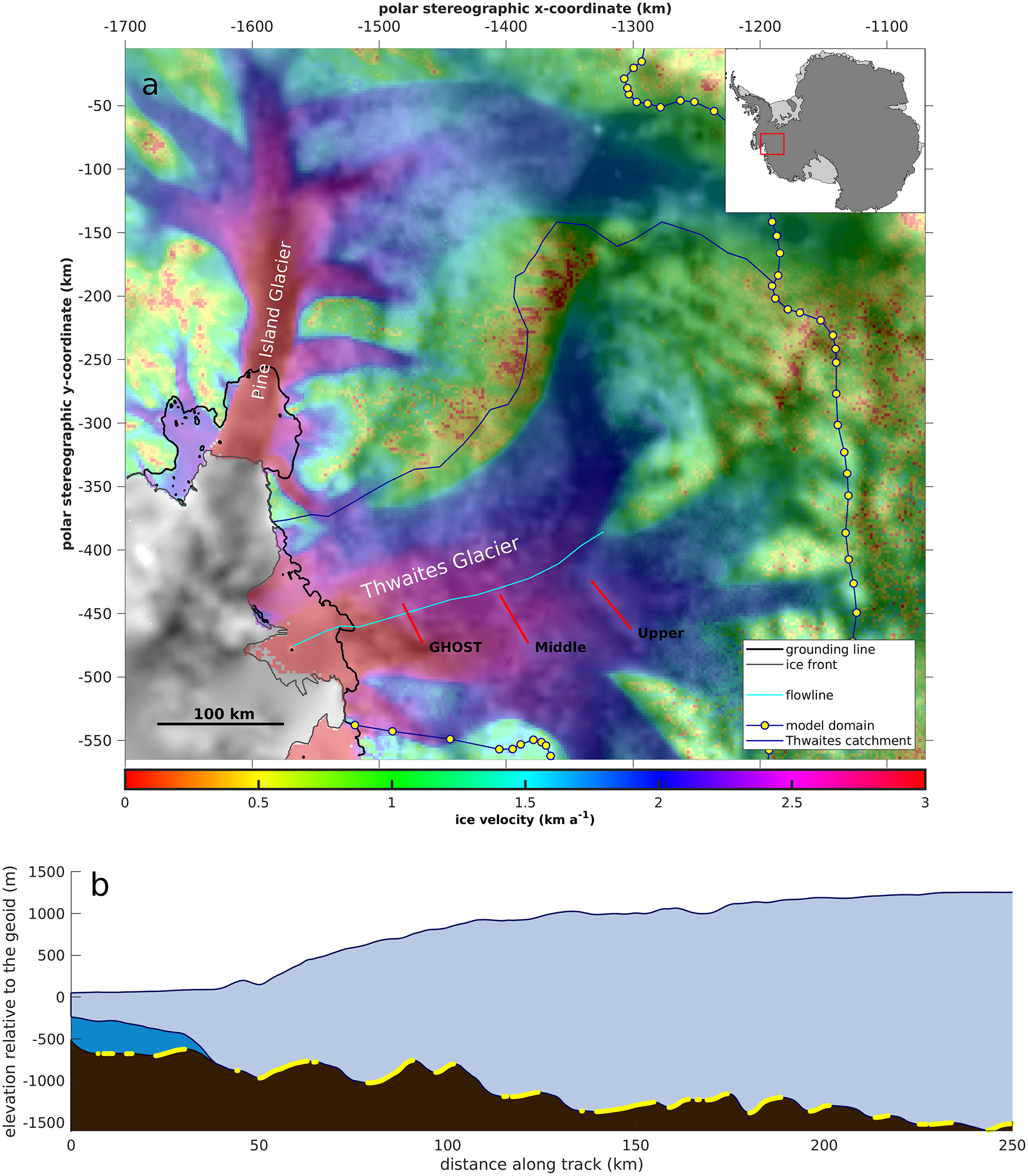
(a) MeASUREsv2 velocities (Rignot and others, Reference Rignot, Mouginot and Scheuchl2017a) in our model domain (blue line with yellow markers) overlain on BEDMAP2 topography. Note that the relative location of (a) is shown on the inset map. Three key transverse ridges beneath Thwaites are highlighted, including GHOST ridge (near x = −1500 km), a second, middle ridge at approximately X = −1400 km, and a third, upper ridge farther inland extending between approximately x = −1350 to −1300 km; the initial grounding-line (bold black), ice-shelf extent (gray), and glacier catchment boundaries (navy), as well as the central flowline sampled in Figure 3 (cyan) are shown. (b) A topography transect along central flowline (cyan) shows areas of the bed (brown) that fulfill our ‘stoss’ criterion (yellow) for inversions.

Figure 1 Long description
The image consists of two parts. The first part (a) is a map showing Thwaites Glacier with polar stereographic coordinates. It highlights the glacier's grounding line, ice front, flowline, model domain and catchment boundaries. Key transverse ridges are labeled as GHOST, Middle and Upper. The map includes a color scale for ice velocity in kilometers per year and an inset map of Antarctica. The second part (b) is a graph showing elevation relative to sea level along a track distance in kilometers. The graph displays areas of the bed fulfilling the 'stoss' criterion, with elevation values ranging from 0 to 1500 meters and distance from 0 to 250 kilometers.
Several transverse bedrock ridges beneath Thwaites Glacier (Fig. 1) associated with the West Antarctic Rift System (e.g. Behrendt, Reference Behrendt1999; Winberry and Anandakrishnan, Reference Winberry and Anandakrishnan2004; Bingham and others, Reference Bingham2012; Alley and others, Reference Alley2021) have the potential to act as stabilizers as its grounding-zone retreats toward the deep interior basins well upstream from its modern location (Morlighem and others, Reference Morlighem2020). Field campaigns (Muto and others, Reference Muto, Alley, Parizek and Anandakrishnan2019a,Reference Muto, Alley, Parizek and Anandakrishnanb; Clyne and others, Reference Clyne, Anandakrishnan, Muto, Alley and Voigt2020; Holschuh and others, Reference Holschuh, Christianson, Paden, Alley and Anandakrishnan2020) as well as modeling studies (Joughin and others, Reference Joughin2009) focused on the bed in ASE have revealed variable bed rheology across these key features. While some areas beneath Thwaites and neighboring Pine Island Glacier consist of a harder material (likely sedimentary bedrock; Alley and others, Reference Alley2021), there are stretches of bed comprising a weaker material (likely meters-thick or greater deformable till; Joughin and others, Reference Joughin2009; Alley and others, Reference Alley2021, Reference Alley2022).
Inversions for basal lubrication (e.g. Joughin and others, Reference Joughin2009) show that poorly lubricated and well-lubricated regions alternate along flow. Coordinated seismic and radar surveys reveal that the well-lubricated regions are soft beds occupying large basins and lee sides of topographic highs, whereas poorly lubricated regions are hard beds that occur primarily on stoss sides of large basal topography (Muto and others, Reference Muto, Alley, Parizek and Anandakrishnan2019a,Reference Muto, Alley, Parizek and Anandakrishnanb; Clyne and others, Reference Clyne, Anandakrishnan, Muto, Alley and Voigt2020). Hard beds also generally extend slightly downstream across peaks of larger subglacial topographic ridges, and may occur in troughs between lee side till bedforms and moats just upstream of larger ridges (Alley and others, Reference Alley2021, Reference Alley2022).
The detailed seismic and radar data were first developed for one region of the bed of Thwaites Glacier (Muto and others, Reference Muto, Alley, Parizek and Anandakrishnan2019a,Reference Muto, Alley, Parizek and Anandakrishnanb), and then tested and found accurate by applying a similar analysis to a region farther downstream (Clyne and others, Reference Clyne, Anandakrishnan, Muto, Alley and Voigt2020). Such data cover only a small part of the whole bed of Thwaites Glacier, however, whereas topography is relatively well known for the entire glacier. We thus assign bed type based on topography. Using a data-driven inversion approach, we utilize bedrock topography and slope to assign a spatially variable sliding-law exponent to prescribe either a linear-viscous or slightly nonlinear model to steep, upglacier-facing beds and a more nearly plastic material elsewhere in prognostic models of Thwaites Glacier. Differences in dynamic response to sustained ocean forcing between mixed basal rheology and more standard homogeneous bed conditions show the influence of this basal boundary condition on glacier dynamics, providing key information to improve existing models seeking to project WAIS’s contribution to sea-level rise.
While bed topography largely controls simulated patterns of retreat on Thwaites, ocean forcing tends to control the pace of this retreat (Seroussi and others, Reference Seroussi2017). Further, the friction law controls the dynamic response of the glacier when it is subjected to forcing. The existence of this topography-driven retreat, as well as the topographically influenced pattern in bed rheology seen in data, therefore points toward a need to consider how this spatially variable boundary condition could affect modeled outcomes.
Under our algorithm for bed-exponent assignment, the upstream side and tops of major topographic ridges beneath Thwaites are prescribed a linear-viscous (or, in separate runs, a slightly nonlinear) bed rheology, while much of the less-prominent topography is set to deform in a more nearly plastic manner. Additional detail might be supplied in the future if bed data with higher spatial resolution are collected. In flowline experiments with prescribed ocean warming, assigning a linear-viscous bed versus a more nearly plastic bed was found to switch the Thwaites grounding zone between retreat and stability, respectively, albeit with mass loss in both cases (Parizek and others, Reference Parizek2013). In our map-plane simulations of Thwaites, both homogeneous bed types produced retreat, but with decadal-scale differences between model runs in the timing of more-rapid retreat pulses (Schwans and others, Reference Schwans, Parizek, Alley, Anandakrishnan and Morlighem2023). Flowline modeling by Koellner and others (Reference Koellner, Parizek, Alley, Muto and Holschuh2019) utilized a mixed bed rheology, showing how the basal flow law can interact with topography and produce results that fall outside those with a uniform rheology. Several other studies have explored the influence that the choice of basal sliding law has on modeled behavior of Thwaites (e.g. Yu and others, Reference Yu, Rignot, Seroussi and Morlighem2018; Barnes and Gudmundsson, Reference Barnes and Gudmundsson2022), but there has been limited research seeking to determine the influence of nonhomogeneous basal rheology in map-plane simulations.
We expand upon previous work by extending a spatially variable ‘mixed’ rheology model into the lateral dimension using bed topography to guide our assignment of the basal sliding exponent, allowing us to explore the influence that this observed variability in bed character could have on the dynamic evolution of Thwaites Glacier.
Methods
The Ice-sheet and Sea-Level System model (ISSM) (Larour and others, Reference Larour, Seroussi, Morlighem and Rignot2012) is used to simulate the retreat of Thwaites Glacier under several configurations for basal rheology and ocean forcing. We implement the two-dimensional (2-D) shallow-shelf approximation (SSA) physics core to model ice flow in ASE, retaining computational efficiency and capturing membrane stresses, but neglecting vertical shear and bridging stresses (MacAyeal, Reference MacAyeal1989). For further insight into limitations arising from this approximation within the context of this study, see Discussion section.
Thwaites’ largest neighboring glacier, Pine Island Glacier, is included in our model domain (yellow/blue marked line, Fig. 1a), and we utilize the same initialization datasets to remain consistent with Schwans and others (Reference Schwans, Parizek, Alley, Anandakrishnan and Morlighem2023), constraining our model as in Schwans and others (Reference Schwans, Parizek, Alley, Anandakrishnan and Morlighem2023), using:
i) ice-temperatures and associated flow-law parameter (Glen, Reference Glen1955) as well as basal melting rates for grounded ice from PSU-3d modern output (Pollard and DeConto, Reference Pollard and DeConto2012)
ii) ice velocities, ice front, and grounding-line locations from (D)InSAR (MeASUREs V2 dataset; Rignot and others, Reference Rignot, Mouginot and Scheuchl2016; Mouginot and others, Reference Mouginot, Rignot, Scheuchl and Millan2017; Rignot and others, Reference Rignot, Mouginot and Scheuchl2017a, Reference Rignot, Mouginot and Scheuchlb
iii) geometry from BEDMAP2 (Fretwell and others, Reference Fretwell2013)
iv) precipitation and accumulation from ALBMAPv2 (Le Brocq and others, Reference Le Brocq, Payne and Vieli2010)
v) no-flow/fixed-flow boundary conditions along the edges of our domain constrained by local ice velocity and thickness (i.e. our model is not configured for drawdown of adjacent basins, limiting the total possible contribution to SLR, e.g. Bamber and others, Reference Bamber, Riva, Vermeersen and LeBrocq2009)
vi) a stress-free ice surface and depth-integrated water pressure at the ice/ocean interface
vii) n = 3 in Glen’s flow law (Cuffey and Paterson, Reference Cuffey and Paterson2010)
viii) a power-law that describes basal sliding (inversion details below)
The mesh used in our ensemble allows for coarse resolution (up to ∼30 km) over Pine Island Glacier, with elements over Thwaites ranging in size from 800 m to 5 km. We tested another mesh that enforces a resolution of ∼2 km across the whole domain (up to ∼4 km) with some elements in fast-flowing areas near the front that scale down to <50 m. Differences in mass-loss arising from this change in mesh are minor (see Supplementary Fig. S1b), allowing us to utilize the lower-resolution mesh for the majority of our experiments.
We further reduce resolution dependency by utilizing built-in parameterizations in ISSM to capture sub-element-scale melt and friction to simulate a grounding zone, which weights either the melt or friction value assigned to a partially floating element according to the proportion of the element that is floating or grounded (Seroussi and others, Reference Seroussi, Morlighem, Larour, Rignot and Khazendar2014). Though ISSM treats the grounding-line as a linear feature, using these parameterizations can capture some transitional-zone behavior and reduce resolution dependency (e.g. Seroussi and Morlighem, Reference Seroussi and Morlighem2018; Yu and others, Reference Yu, Rignot, Seroussi and Morlighem2018). We note, based on findings of a variable and extensive grounding zone on Thwaites Glacier (e.g. Parizek and others, Reference Parizek2013; Rignot and others, Reference Rignot, Ciracì, Scheuchl, Tolpekin, Wollersheim and Dow2024), this remains a conservative representation of grounding-zone ice-ocean processes (Parizek, Reference Parizek2024) and therefore of grounding-zone retreat rates. Yet it serves as a useful means of comparison with prior results (Schwans and others, Reference Schwans, Parizek, Alley, Anandakrishnan and Morlighem2023) in order to build process understanding associated with the choice of basal rheology.
Models are forced by sub-shelf melt rates from ROMS output in the ASE (St-Laurent and others, Reference St-Laurent, Klinck and Dinniman2015), which drive retreat in our simulations. Inland of the MEaSUREs V2 grounding-line location (solid black line, Fig. 1a), we extrapolate one of two reasonable front-proximal melt values to create two static ocean conditions that we utilize in our model ensemble. Newly ungrounded ice over Thwaites is forced with a melt-rate of either 40 m a−1 (low-value static ocean [LSO]) or 100 m a−1 (high-value static ocean [HSO]) in 500-year forced transient runs (Schwans and others, Reference Schwans, Parizek, Alley, Anandakrishnan and Morlighem2023).
Prior to applying this forcing, we perform a relaxation transient to reduce numerical noise from nonconcurrent datasets, updating our geometric fields at the end of the relaxation period while retaining original velocities from the MEaSUREs V2 dataset. Our initialization workflow also includes an inversion for ice-rheology on Thwaites’ floating shelf to aid in obtaining a better result in friction fields near the grounded-to-floating transition while using SSA physics (Borstad and others, Reference Borstad, Rignot, Mouginot and Schodlok2013). SSA has a tendency to increase inverted friction values near the grounded-to-floating transition if floating-ice stiffness is simply assigned using temperature fields. An inversion for stiffness on the ice-shelf allows us to reproduce high speeds near the grounding-line without artificially increasing basal friction in our model set-up.
Two sets of inversions (with one set comprising separate inversions for the frictional drag coefficient and the flow-law parameter) are conducted for each respective basal friction set-up—one set before and one set after the relaxation transient—before running forced transients. This reduces the misfit in the second set of inversions (i.e. our initial state for forced runs) by virtue of having a consistent, more-constrained initial state for our relaxation transient.
In order to allow for a mixed bed, friction is prescribed on an element-wise basis, rather than a vertex-wise basis as is usually done in ISSM. Differences between models run with a vertex-wise assignment of basal friction and those with an element-wise assignment are negligible (see Supplementary Fig. S1a for further details).
Basal ice velocity ( ${v_{\text{b}}}$) is normally related to shear stress at the ice/bed interface (
 ${{{\tau }}_{\text{b}}}$) using a drag coefficient (Cuffey and Paterson, Reference Cuffey and Paterson2010),
 ${\text{ - }}{{{\alpha }}^{\text{2}}}$, for which we invert prior to running our model forward. In the simplest formulation, the exponent in this equation, m, describes how the bed responds to changes occurring in ice that is sliding above:
 \begin{equation}{{{\tau }}_{\text{b}}}{\text{ = - }}{{{\alpha }}^{\text{2}}}{{\text{v}}_{\text{b}}}^{{\text{1}}/{{m}}}\end{equation}
Various complexities can be added, such as a yield stress, a maximum (Iken) stress, or a dependence on water pressure, but we start with the simplest case. Physical models exist (Cuffey and Paterson, Reference Cuffey and Paterson2010) that range from m = 1 (viscous sliding, appropriate for Weertman-style sliding dominated by regelation) up to m tending toward infinity (appropriate for some soft tills). In earlier works (Schwans, Reference Schwans2018; Koellner and others, Reference Koellner, Parizek, Alley, Muto and Holschuh2019), we have used m-values of 1, 3 and 8, and then focused on 1 and 8. Higher values than 8 tend to introduce numerical instability without greatly changing the results, and the larger contrast between behavior with m = 1 and m = 8 proved to be more instructive than comparisons involving m = 3. Therefore, we use m = 1 and m = 8 in our main simulations here, but include several runs using m = 3 and m = 8 to provide additional insights. m is used to initialize the inversion, and remains fixed throughout transient runs.
Here, we refer to the m = 1 bed as ‘hard’ or ‘bedrock’. Although Weertman sliding is typically used in models to prescribe motion over a nondeformable substrate, it is more likely that these bedrock ridges would be more aptly described by m = n = 3—i.e. regelation is likely not controlling motion over these very large features in the bed, and thus the exponent by which shear-stress and basal velocity are linked is constrained by ice deformation according to Glen’s flow (Cuffey and Paterson, Reference Cuffey and Paterson2010). (We do not pursue the further possibilities of n = 4 or spatially variable n in Glen’s flow law.)
Translating the observed lee/stoss variability in bed rheology into our model of Thwaites requires extrapolating this pattern across the extent of our model domain. We utilize the slope of the bed in the down-flow direction to assign m in our mixed-bed simulations across the entirety of our model domain. In areas where this down-flow slope exceeds .01, we assign our ‘stoss’ criterion, setting our m equal to either 1 or 3; elsewhere, we prescribe our more nearly plastic condition (m = 8). The result provides a good approximation of a soft/hard lee/stoss pattern in our friction-exponent field (Fig. 1b), where the upstream sides of most bumps larger than ∼100 m are prescribed a low exponent, while the downstream sides of bumps as well as more nearly horizontal portions of bed, are set to m = 8.
With little data on the uppermost Thwaites to verify that this pattern persists there, we include two additional intermediate mixed-bed scenarios. These hybrid beds treat this deep upstream zone (where bed is deeper than −1300 m) as though it is underlain by a homogeneous substrate with either chosen endmember rheology, while prescribing variable rheology throughout the rest of the catchment according to our lee/stoss criteria above.
In our main ensemble, we test five different element-wise basal-friction configurations:
i) Homogeneous assignment of a linear-viscous bed (m1)
ii) Homogeneous assignment of a slightly nonlinear bed (m3)
iii) Homogeneous assignment of a more nearly plastic (‘plastic’) bed (m8)
iv) Slope-dependent assignment (SDA) of m = 1, m = 8 (mixed18)
v) SDA of m = 3, m = 8 (mixed38)
vi) SDA with inland areas deeper than −1300 m prescribed as linear-viscous (mixed18_1)
vii) SDA with inland areas deeper than −1300 m prescribed as more nearly plastic (mixed18_8)
To invert for either the basal friction coefficient,  ${{{\alpha }}^{\text{2}}}$, or the flow-law parameter, B (Glen, Reference Glen1955), ISSM utilizes an adjoint method, iteratively solving a forward problem to minimize the misfit between observed and modeled ice velocities. This results in an inverted field that best reproduces observations while operating within user-defined parameters for smoothness, error, and more (Morlighem, Reference Morlighem2011). Our parameters in each inversion are assigned and scaled according to our prescribed spatial distribution of m, and our cost function includes both an absolute and logarithmic misfit component to better capture transitions in ice velocity across Thwaites. Cost-function weights (Supplementary Table S2) and parameters used in inversions were mainly determined by trial and error to obtain an acceptably small misfit for each full inversion (more details on inversion and workflow can be found in Supplementary Material).
Prior to inversion, we initialize an a priori field by setting basal drag equal to driving stress. This provides a reasonable initial guess for both homogeneous beds and the slope-dependent mixed beds. However, intermediate mixed-bed scenarios (where deep inland areas are treated as homogeneous) required a different approach to obtain a smaller misfit, particularly in the first friction inversion prior to the relaxation transient. These hybrid mixed18_1/mixed18_8 inversions were instead initialized by rescaling the  ${{{\alpha }}^{\text{2}}}$ distribution derived from our linear-viscous inversion result to create a more suitable initial guess and obtain a smaller misfit for these two sliding-law exponent distributions.
Our topography-driven SDA of rheology results in a bed that largely consists of a more nearly plastic material interspersed with areas of linear-viscous bed where topography is sufficiently steep. Over the tops and along the upstream-facing sides of major topographic ridges, our stoss assignment criterion creates larger, more continuous stretches of linear viscous deforming bed (Fig. 1b). This same distribution holds true in our mixed38 simulations, but with m = 3 assigned on stoss sides instead. M-distributions and mismatches can be found in the Supplementary Materials.
After going through a full inversion to obtain  ${{{\alpha }}^{\text{2}}}$, each bed experiment is run forward for 500 years under each ocean forcing to compare responses and constrain the level of influence of a mixed bed rheology on Thwaites Glacier. Note that many processes that could be important to retreat rate are not included in this model, such as full ice-shelf loss, meltwater wedging of surface crevasses, or ocean water circulating inland of the grounding-line in an estuarine system. Thus, the results should not be viewed as a projection of future sea-level rise. Instead, this is a sensitivity experiment to determine whether the forced response is significantly impacted by including a spatially variable flow law.
Results
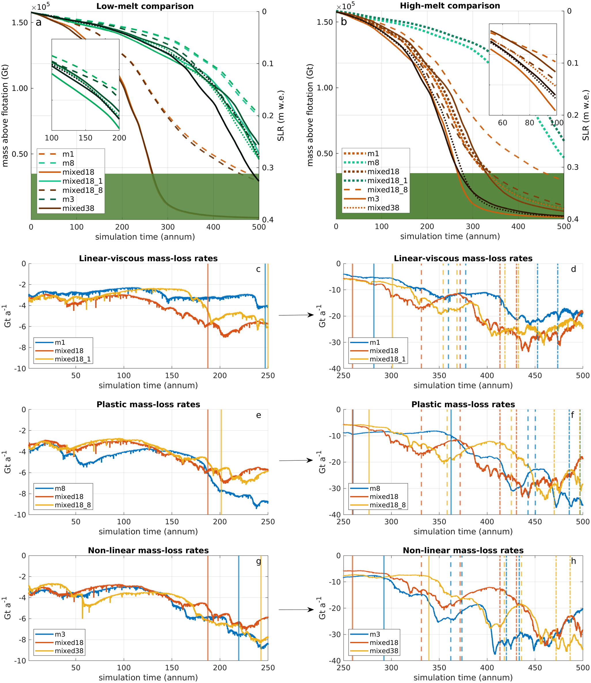
In all models, Thwaites retreats far into its catchment, contributing to sea-level rise at a rate that is affected by prescribed bed rheology and ocean forcing (Fig. 2). The timing of significant changes in mass-loss rates (Fig. 2c–h) differs among each bed and ocean prescription, and is linked to retreat over major ridges beneath Thwaites. We summarize retreat rates for each rheology set-up in Supplementary Table S1, and calculate mass-loss rates in Fig. 2 using a centered-difference scheme, using vertical lines to illustrate inland motion of the grounding-line. Specifically, we demarcate its migration onto and off of the highest point of each major ridge along our central flowline (Fig. 1). In this section, we first discuss general patterns seen in mass-loss and retreat style for each bed. We compare our homogeneous experiments to put our mixed/hybrid bed experiments into context, then go into details of the differences among modeled grounding-line retreat rates and surface-height evolution between experiments.
(a–b) Ice mass above flotation throughout the modeled period in Thwaites’ catchment (delineated in Figure. 1a by the solid blue line and corresponding domain-edge) using both sub-shelf melt conditions (a: 40 m a−1; b: 100 m a−1) for newly ungrounded elements within our main model ensemble. Insets show detail for selected portions of transients where ice mass begins to diverge. The green box designates where modeled rates of mass loss begin to be limited by our fixed flow conditions at the boundary of our domain (see Results section for details). (c–h) show centered-difference for ice mass above flotation for each homogeneous (blue) bed, our mixed18 (red) and either the corresponding hybrid bed for m1 and m8 (yellow, panels c–f) or mixed38 (yellow, panels g and h) throughout our transient run forced with 40 m a−1 sub-shelf melt rates beneath newly ungrounded ice. Note that runs are broken up into two panels each to better illustrate ice mass trends throughout these transients, with different y-scales as the transient progresses. Vertical lines coincide with the GL’s arrival at and departure from the highest point on each major ridge along our central flowline (Figure. 1a). Solid lines are for motion onto/off of GHOST, dashed lines for the middle ridge, and dash–dot lines for motion onto and off of the furthest-inland transverse ridge in Figure. 1a.

Figure 2 Long description
The image contains six graphs comparing ice-mass loss rates under different conditions. The top row shows two graphs: 'Low-melt comparison' and 'High-melt comparison'. Both graphs plot 'mass above flotation' in gigatons on the left y-axis and 'SLR' in meters on the right y-axis against 'simulation time' in annum on the x-axis. The low-melt graph includes curves for m1, m8, mixed18, mixed38 and hybrid beds, while the high-melt graph includes m1, m8, mixed18, mixed38 and hybrid beds. The middle row shows 'Linear-viscous mass-loss rates' for low and high melt conditions, with 'mass-loss rates' on the y-axis and 'simulation time' on the x-axis. The bottom row shows 'Plastic mass-loss rates' and 'Non-linear mass-loss rates' for both conditions, with similar axes. Each graph includes multiple curves representing different bed conditions, with vertical lines indicating specific events or transitions. The graphs illustrate trends and differences in ice-mass loss over time under varying melt conditions and bed types.
In each transient, Thwaites’ grounding-line generally migrates faster over areas between ridges, while motion up to and over large ridges is relatively slower (Alley and others, Reference Alley, Anandakrishnan, Dupont, Parizek and Pollard2007; Parizek and Walker, Reference Parizek and Walker2010). At several points throughout our forced runs, Thwaites becomes ungrounded from larger inland bed features, such that retreat proceeds swiftly along deep retrograde areas between transverse ridges. The timing of the onset of these periods of accelerated inland grounding-line migration differs among our bed-exponent and ocean-forcing assignments. In every scenario, unstable retreat initiates when the grounding-line has migrated past Upper Thwaites Ridge (Fig. 1) within our modeled period. At this point, Thwaites begins to recede rapidly at a rate that becomes limited by fixed boundary conditions as the grounding-line approaches the edges of our modeled domain. The influence of rheology on modeled mass-loss becomes weaker at this stage—mass-loss decelerates by virtue of fixed inflow at our domain boundary rather than as a result of bed rheology choice. Note that the domain boundary stops retreat in our simulations; it would not do so in the real ice sheet.
Homogeneous beds
Thwaites consistently experiences faster mass loss while sliding over a homogeneous plastic bed (m8) compared to a homogeneous linear-viscous bed (m1) throughout both LSO- (Fig. 2a) and HSO-forced (Fig. 2b) 500-year transients with element-wise rheology. Runs with slower sub-shelf melt (Fig. 2a, 2c–h) show substantial mass-loss acceleration after several centuries of forcing when we use any homogeneous bed prescription (Fig. 2c–h, blue curves).
Low ocean forcing
Under our plastic condition (Fig. 2a, m8, solid light teal line), the first large increase in the rate of Thwaites’ contribution to sea-level rise occurs after ∼180 years of LSO forcing (Fig. 2e, m8, blue curve), with a second, more marked speedup initiating around 350 a into the transient when the grounding-line begins to pull off of GHOST ridge (Fig. 2f). The grounding-line proceeds slowest over m8, migrating over GHOST ridge for much of the simulation as ice is readily flushed from far upstream in Thwaites’ catchment (Fig. 2e, f). After losing contact with GHOST ridge around 350 years into the transient, Thwaites begins losing mass rapidly in this scenario, with the grounding-line lagging over subsequent ridges for a very limited time, as inland reserves of ice have been depleted and ice thickness is closer to flotation.
With a linear-viscous bed (Fig. 2a, m1, dashed light teal line), Thwaites’ mass-loss speeds up more gradually throughout the transient, with a notable increase in mass-loss rates after ∼300 years of LSO forcing, following grounding-line departure from GHOST ridge (Fig. 2d, blue curve). Another bout of mass-loss acceleration can be seen after almost an additional century of forcing m1 following grounding-line departure off the second ridge (circa 415 years into LSO-driven transient) (Fig. 2d, blue curve).
The slightly nonlinear bed (m3) initially falls between endmember cases, but under sustained forcing, proceeds to lose mass faster than homogeneous endmembers under weaker sub-shelf melt (Fig. 2a, darkest solid curve). This acceleration occurs after about three centuries of LSO forcing such that, after ∼330 years, m3 overtakes m8. The m3 grounding-line reaches GHOST ridge sooner than in simulations using either m1 or m8 (Fig. 2g, h), reaching the central ridge around the same time as m1, but subsequently pulling off more quickly from both the central and upper ridges beneath Thwaites under sustained forcing.
High ocean forcing
Our higher-temperature ocean condition shows the same general mass-loss trends for each homogeneous bed (Fig. 2b). Mass loss under m8 accelerates after about 70 years of HSO forcing, and again after about 175 years of HSO forcing as the grounding-line moves off of the GHOST ridge (see Supplementary Material for details of timing of GL migration for HSO results). With m1, we see minor mass-loss acceleration ∼140 years into the transient, with more substantial mass-loss acceleration occurring after ∼220 years of stronger ocean forcing. Our model with an m3 bed starts to lose mass faster than homogeneous endmembers after about 180 years of HSO forcing.
Mixed beds
With more gradual sub-shelf melt, modeled mass-loss over our mixed bed with linear-viscous stoss-sides (Fig. 2a, mixed18, dotted light teal line) first trends between mass-loss curves of the two endmember homogeneous beds before accelerating after about ∼290 years of LSO forcing (Fig. 2d, e, yellow line). Eventually, this overtakes mass-loss arising from m8 (Fig. 2a, solid light teal line) around 350 years into the transient run. When melt-rates are higher, however, the mass-loss modeled with a mixed18 bed consistently falls between those of our homogeneous endmember cases (Fig. 2b).
When we instead assign a stoss criterion of m = 3 (Fig. 2a, mixed38, dotted dark teal line), mass-loss falls outside of the envelope bounded by homogeneous runs using either m3 or m8 under both ocean forcings. Our mixed38 bed results show slower mass-loss over Thwaites than m3 or m8 during the 3rd century of LSO forcing (Fig. 2a), and after ∼150 years of HSO forcing (Fig. 2b). While modeled mass-loss is comparable throughout the first two centuries of weaker ocean forcing regardless of which exponent value is assigned on the stoss-sides of large bed features (Fig. 2a, dotted lines), mixed38 produces slower mass-loss during the third century of LSO forcing, lagging mass-loss modeled using the mixed18 bed after ∼315 years.
Differences in grounding-line retreat timing onto and off of major ridges are seen between our two fully mixed-bed scenarios using SDA of rheology (yellow curves in Fig. 2c, d or Fig. 2e, f vs Fig. 2g, h). Our simulation with mixed38 allows the grounding-line to migrate over GHOST ridge slowly compared to that with mixed18, such that the grounding-line retreating over a mixed18 bed reaches the middle ridge beneath Thwaites before the grounding-line in the mixed38 scenario has left GHOST ridge under the same low ocean forcing.
Hybrid beds
Experiments utilizing a mixture of our SDA algorithm and homogeneous endmember rheology in deep upstream areas (e.g. mixed18_1 and mixed18_8, darker teal and orange dashed and solid lines in Fig. 2a, b) illustrate that changes in how the far-inland bed balances stresses can alter the rate at which Thwaites contributes to sea-level rise throughout transient runs. Overall, these hybrid-bed models show differences in both the magnitude and the timing of the onset of mass-loss acceleration (Fig. 2c–f, red curves), as well as differing capacities for (ephemeral) restabilization of Thwaites’ grounding-line throughout its retreat when compared to either mixed18 or mixed38 (yellow curves in Fig. 2c–f; yellow and red in 2g–h) or any homogeneous bed rheology (m1, m3, m8; blue curves in Fig. 2c–h).
When inland sub-shelf melt is set to 40 m a−1, through the first century, the mixed18_1 shows a similar mass-loss trajectory to that of m1 (Fig. 2a, lighter dashed line). After ∼170 years of forcing, mass-loss over mixed18_1 (Fig. 2c, red curve) accelerates relative to that of m1, after which the mass-loss trajectory begins to trend with that of the mixed18 bed (Fig. 2a, dotted light teal line), though showing slightly less total mass loss. However, stronger ocean forcing causes faster mass loss with mixed18_1 (Fig. 2b, dark dashed orange line) compared to mixed18 (Fig. 2b, dotted orange line).
For mixed18_8 (Fig. 2b, solid dark teal line), mass-loss rates are consistent with those over our mixed18 bed until ∼260 years into the LSO-forced transient. At this point, mass loss over mixed18 (Fig. 2f, yellow curve) accelerates relative to mixed18_8 (Fig. 2f, red curve). The hybrid bed starts to experience faster mass loss only after more than ∼340 years of LSO forcing, and, once again, Thwaites generally retains more ice mass over the course of the transient than when we use this SDA of rheology prescription throughout the whole catchment.
Time-evolution of rate of mass-loss in the mixed18_8 scenario is highly sensitive to topography, as the grounding-line retreats rapidly across lowlands and (temporarily) re-stabilizes on topographic highs (Fig. 2e, f, red curve). This becomes more apparent under high-melt forcing: mass-loss for mixed18_8 shows clear phases of retreat in which mass loss slows as the grounding-line stabilizes on major transverse ridges, then strongly accelerates as the grounding-line moves off of these features (Fig. 2b, solid light brown curve).
These results demonstrate how distal, inland swaths of bed with either endmember rheology (linear-viscous or more nearly plastic) can alter modeled contribution to sea-level rise, even when the main trunk of Thwaites in these experiments retains the same lee/stoss pattern in a linear-viscous vs plastic bed rheology distribution. When ocean forcing is lower, mixed18 enhances modeled mass loss rates compared to either m1 or m8 alone (Fig. y2a). Further, the precise distribution of m (i.e. whether a mixed-material bed persists across the entirety of Thwaites’ catchment) can significantly affect modeled retreat on Thwaites (Fig. 2b).
Surface-profile evolution
While using a higher value for sub-shelf melt can reduce the influence the bed has on modeled mass loss, simulations using a low ocean forcing are more instructive to process understanding, allowing us to analyze the differences arising from bed-driven retreat behavior, particularly when we look at the evolution of surface height along the central flowline of Thwaites (Fig. 3). That is, differences in modeled retreat among experiments are most prominent when our ocean forcing is weaker and allows for gradual dynamic adjustment to prescribed melt.
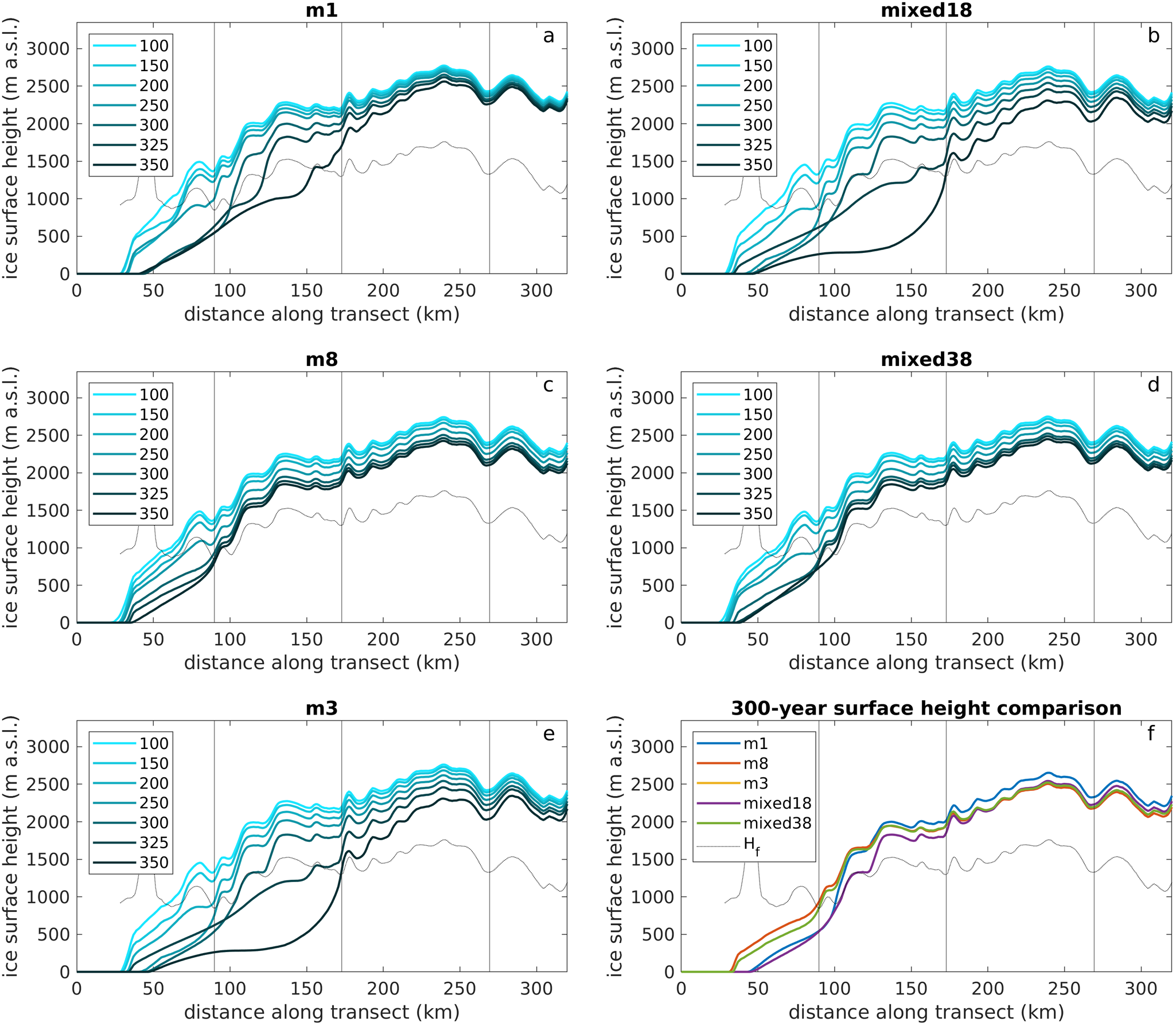
(a–e) Surface-height progression along chosen central flowline over Thwaites (cyan line, Figure. 1a) under LSO forcing for each bed type. Legend designates model year for each respective profile. Flotation height is designated by the thin, lighter line, while each major bedrock ridge (Figure. 1) is demarcated with a solid vertical line. (f) A comparison of all surface profiles at the 300-year mark.

Figure 3 Long description
The image contains six graphs labeled a to f. Graph a shows 'm1' with ice surface height (m, a.s.l.) on the y-axis and distance along transect (km) on the x-axis, displaying lines for years 100 to 350. Graph b shows 'mixed18' with similar axes and year lines. Graph c shows 'm8' with the same axes and year lines. Graph d shows 'mixed38' with similar axes and year lines. Graph e shows 'm3' with the same axes and year lines. Graph f is a 300-year surface height comparison for models m1, m8, m3, mixed18 and mixed38, with the same axes. Each graph includes a legend indicating model years for each profile.
As found in Schwans and others (Reference Schwans, Parizek, Alley, Anandakrishnan and Morlighem2023), upstream ice remains thicker when sliding over an m1 bed than over m8, though there is more thinning near the front (Fig. 3a vs 3c). While m1 initially allows the grounding-line to remain stable on high points for some time (Fig. 2c, d, blue curve), further mass loss from sustained forcing along with higher driving stresses causes inland retreat to proceed earlier than in runs with m8. Though m8 allows lower surface slopes and associated driving stresses, retreat eventually proceeds faster (though it initiates much later) under sustained forcing as the grounding-line moves back into a thinner catchment.
The nonlinear case (i.e. m = 3) operates in the middle of this spectrum of behavior, which appears to have a destabilizing effect on Thwaites when compared to either homogeneous endmember rheology. Thinning patterns modeled when using m3 (Fig. 3e) fall between endmember cases, in that m3 still balances stresses more locally than m8, but more distally than m1. This results in both far-field drawdown and localized surface steepening near the grounding-line throughout the transient (Fig. 3e), eventually producing faster mass loss under sustained forcing (Fig. 2a, solid black line). The timing of grounding-line arrival and departure from major ridges over homogeneous beds shows how m = 3 behavior results in an evolving trade-off between limiting initial grounding-line motion by virtue of increased ice-flux to the grounding-line and enhanced rates of local drawdown (see Supplementary Table S1 for comparison of grounding-line motion across bed experiments). Under LSO forcing, the grounding-line migrating over m3 (Fig. 2g, h) reaches GHOST ridge sooner, but departs slightly later than the m1 grounding-line (Fig. 2c, d). Though both reach the middle ridge at about the same time, grounding-line departure from this ridge occurs about half a decade sooner with m3, with subsequent migration up to and off of the last major transverse ridge occurring decades in advance of the m1 grounding-line. Having depleted much of the catchment’s upstream ice to balance stresses while also retaining steeper surface slopes that drive higher ice flux across the grounding-line than for flow over m8, m3 produces a combination of dynamics that results in the fastest average retreat over Thwaites among homogeneous bed experiments under either ocean forcing.
The spatial pattern of simulated surface-height changes modeled using mixed18 provides insights into the reasons for faster retreat with a mixed bed than with a uniform bed under the same forcing (Fig. 3b). Extensive areas of softer bed draw down much of the basin in response to sub-shelf melt. Simultaneously, linear-viscous stretches of bed preferentially restrict thinning just upstream of high points in Thwaites’ bed topography, limiting the availability of local ice for adjacent plastic areas of the bed to draw from. This further enhances distal drawdown over mixed18 relative to that observed over m8 (Fig. 3b vs 3c). Under sustained forcing, this blend of bed-driven thinning creates both steeper ice surfaces near high points in the bed and relatively thinner ice throughout the catchment (Fig. 3c). Higher driving stresses near stabilizing bed features and more widespread thinning combine to cause faster inland grounding-line migration over a mixed18 compared to any homogeneous rheology scenario.
Further, m1 shows relatively more ice thickness remaining atop these large topographic highs in the bed, but with lower surface slopes when compared to our mixed18 bed that includes a transition in both form and dynamic drag (Fig. 3a vs 3b; ridge locations along-flow marked with vertical lines). That is, the widespread drawdown signature characteristic of m8 still persists in our mixed bed runs, but is combined with the thinning fingerprint that results from assignment of linear-viscous sliding over high points in basal topography. This dynamic convolution creates our differences in modeled inland grounding-line migration across our bed scenarios under the same static ocean forcings.
After 200 years of LSO forcing, Thwaites’ grounding-line migrating over the mixed18 bed has reached the first major transverse ridge (Fig. 2c–f, yellow curves). At this point in the transient, surface slopes as well as driving stresses near the grounding-line are greater in this scenario compared to either m1 or m8 (Fig. 3b vs 3a, 3c). Under sustained forcing, higher driving stresses combined with widespread drawdown allow the grounding-line to progress inland faster over a mixed18 bed, reaching the farthest-inland transverse ridge around ∼425 years into the LSO-driven run.
Though the m3 produces similar thinning patterns to mixed18 (Fig. 3e vs 3b), topographic highs in m3 do not preferentially retain as much ice thickness as when these areas are prescribed as linear-viscous in a mixed-bed scenario. While both the homogeneous nonlinear and mixed18 beds show faster mass loss and retreat than endmember homogeneous rheology cases, the nonlinear bed does not produce the segmented dynamic response a mixed bed-rheology can create with both its form and dynamic drag transitions, thereby allowing driving-stresses to remain relatively lower over high points in topography (Fig. 3f). Further, m3 simply does not create as steep of surface slopes (Fig. 3e) as m1 (Fig. 3c) when balancing stresses. Our mixed38 results show how the extensive areas of plastic bed dominate the thinning signal (Fig. 3d), and, while nonlinear sections of bed over areas with steep, stoss-side bed topography do retain relatively higher driving stresses than m3, they do so to a lesser extent than mixed18. That is, the areas of nonlinear bed do not produce the same response as in the linear-viscous case (retaining thickness to the detriment of adjacent softer areas of bed), instead allowing Thwaites to lose relatively more ice thickness over regions nearer to the grounding-line as it retreats. This limits how much the soft portions of the bed have to compensate for, which necessitates less catchment-wide drawdown over the mixed38 bed to balance stresses compared to a mixed18 bed. A mixed 38 bed instead appears to limit grounding-line motion and mass-loss when compared to m3 (Fig. 3f).
Discussion
Thwaites is distinctive in flowing across the high-amplitude topography of the West Antarctic Rift System, whereas most ice streams flow along topography. The form drag of the Thwaites subglacial topography exerts major control on ice flow in all of our simulations, and in simulations by other models (e.g. Joughin and others, Reference Joughin2009; Seroussi and others, Reference Seroussi2017). When retreat is forced, it proceeds slowly up slopes on topographic highs (sills), then rapidly down steep slopes, with fairly rapid retreat across deep basins. Ice-surface slopes are relatively steep over basal topographic highs, driving faster flow in the thinner ice there to maintain continuity, which tends to suppress forced grounding-line migration because notable thinning is required to cause small retreat, with grounding-lines migrating more rapidly across topographic basins with smaller ice-air surface slopes.
The sliding rule (Eqn 1) used to specify the dynamic drag modifies this behavior without fundamentally changing it. With a high stress exponent, shear stress cannot be raised much without a huge velocity increase, so reduced buttressing from enhanced sub-ice-shelf melting causes velocity increases that propagate rapidly inland with minimal near-coastal thinning. The minimal thinning causes grounding-line retreat to be small, while the rapid drawdown over much of the inland area contributes to rapid sea-level rise (see, e.g. Sun and others, Reference Sun2020). With a low stress exponent, loss of ice-shelf buttressing is balanced by increased basal shear stress developed by coastal thinning, favoring grounding-line retreat but not drawing down mass rapidly from far inland. This observed behavior in our output is consistent with prior studies using various values for m on Thwaites (e.g. Barnes and Gudmundsson, Reference Barnes and Gudmundsson2022). And, with a mixed bed assigned with a low stress exponent on stoss sides and topographic highs, and high stress exponent on lee sides and across broad topographic plains, forcing favors retreat across the topographic highs and then rapid retreat across the topographic basins with their very low surface slopes, producing faster retreat and mass loss under some parameter combinations than for either endmember, although falling between the endmembers for other combinations.
In our m = 1/m = 8 mixed-rheology assignment, high areas in basal topography tend to sustain increased driving stresses due to their linear-viscous bed rheology, the transition in dynamic drag, and the form drag they provide, while extensive flatter areas across Thwaites’ catchment undergo widespread thinning, causing faster inland grounding-line motion across key stabilizing features.
As the grounding-line approaches major inland ridges from the lee side, it migrates over a prograde plastic bed. However, as the underlying bed just upstream of grounded ice consists of a harder, linear-viscous material, local compensation begins to steepen the ice-surface downglacier of the topographic high. This ridge-top ice acts almost parasitically in these models, retaining ice mass proximally while adjacent plastic areas are drawn down more vigorously in an attempt to balance this localized response. When the bed is entirely plastic, this distal drawdown allows for grounding-line stabilization on high points such that inland retreat is fairly slow as ice is flushed efficiently from elsewhere in the catchment. With more isolated patches of soft bed interspersed between hard ridges, this stabilization mechanism is limited.
However, when we instead use a nonlinear stoss-side criterion, there is less of a trade-off between ice-retention/drawdown over adjacent areas of harder/softer bed. This leads to slower retreat over a bed with m = 3/m = 8 mixed-rheology than over a homogeneous nonlinear bed and slightly faster retreat than over a homogeneous, more nearly plastic bed.
While Parizek and others (Reference Parizek2013) found intermediate ‘stable’ configurations for a flowline Thwaites with a more nearly plastic rheology, we find that including the lateral dimension does not allow for the glacier to reach a stable configuration with our model set-up. Koellner and others’ (Reference Koellner, Parizek, Alley, Muto and Holschuh2019) idealized flowline models demonstrate how the wavelength of the topography in conjunction with rheology distribution can switch behavior between retreat and stability, but in our 2-D configuration using topography data, grounding-line motion in the lateral dimension does not allow for Thwaites to stabilize.
The strength of influence of a mixed bed on modeled outcomes depends somewhat on ocean forcing. Difference in mass loss and grounding-line retreat rates/patterns arising from bed exponent assignment between mixed and homogeneous beds is less pronounced when the ocean is melting more vigorously near the grounding zone. In this case, retreat occurs too rapidly to allow enough time for dynamic adjustment to create a marked difference in bulk behavior (e.g. Waibel and others, Reference Waibel, Hulbe, Jackson and Martin2018). When melted too vigorously, Thwaites is not afforded as much time to create extra-steep surface slopes despite spatial variability in bed rheology, and therefore retreats at a rate controlled by melt and overall dynamic ‘fingerprint’ associated with bulk linear-viscous, nonlinear, or plastic behaviors, rather than producing a retreat-enhancing dynamic feedback. However, it is important to note that a mixed18 bed produces relatively slower mass loss (and contribution to sea-level) under our more vigorous ocean forcing (Fig. 2a, orange dotted line) than a bed that is treated as entirely plastic (solid orange line) or nonlinear (dark brown solid line), as intermittent linear-viscous sections of bed limit the area that soft patches of bed are able to draw from. When we then increase the sliding exponent over stoss-side areas and compare our two SDA mixed beds, we see relatively slower retreat in mixed38 runs when ocean forcing is low (Fig. 2a, dark brown dotted line), but faster retreat than on our mixed18 bed when ocean forcing is stronger. So, while the ability to draw ice from farther upstream is beneficial when enough time is afforded for dynamic adjustment, more vigorous sub-shelf melt negates this benefit, and a bed that more readily evacuates ice from upstream causes faster retreat (Fig. 2b). Furthermore, our experiments assigning a homogeneous plastic rheology in far-inland places beneath Thwaites in conjunction with a mixed bed elsewhere highlight how this ill-constrained condition can produce distinct trajectories of mass-loss on Thwaites even when ocean forcing is enhanced near the front of the glacier (e.g. mixed18_8 in Fig. 2b).
Though the bed-exponent assignment may not act as a strong control once tipping points are reached, results show how upstream rheology can influence mass-loss rates even while the grounding zone is retreating across downstream areas. With unknown rheology in potential retreat pathways into the interior of the Weddell Sea and Ross Sea Embayments, namely through the Byrd Subglacial Basin and Bentley Subglacial Trench, it is clear that accurately representing this basal condition is necessary to reduce uncertainty in future projections from larger ice-sheet models of the WAIS’ contribution to sea-level rise on several scales.
Conclusion
We ultimately find that including a data-informed, topographically dependent mixed bed character with high contrast between sliding exponents predisposes Thwaites’ catchment to higher sustained driving stresses during its retreat. It does this by virtue of both enhanced inter-ridge drawdown from isolated softer swaths of bed, and the tendency for ridge-proximal retention of ice thickness over harder stretches of bed. Under persistent (low) ocean forcing, this dynamic combination leads to enhanced steepening of the ice surface, particularly near major stabilizing ridges. When ocean forcing is more vigorous, the time afforded for drawdown is diminished, such that retreat occurs too rapidly and limits the creation of these extra-steep slopes and associated higher driving stresses.
Increasing the sliding exponent over stoss-sides of large bed features produces slower retreat under low ocean forcing and faster retreat under more vigorous melt, highlighting how complex thinning patterns arising from more-realistic realizations of the bed can produce unexpected outcomes. It is therefore particularly important to incorporate more field data to help guide inversions for basal conditions in order to further reduce uncertainty in predictive models of this key outlet glacier.
More broadly, we note that prior work has shown that the choice of model is the most important source of uncertainty in the projection of future sea-level rise from Antarctica (Seroussi et al., Reference Seroussi2024), and that the basal sliding law may be the most important difference between models (e.g. Sun et al., Reference Sun2020). Models almost always specify a single sliding law for the whole domain. Where geophysical data are available (reviewed in, e.g. Alley et al., Reference Alley2021), they show spatial variations in the nature of the bed between hard bedrock and soft tills (as well as localized lakes, which are not considered further here because of their small size, but which can be important in some cases). Understanding gained from field and laboratory experiments and physical reasoning indicates that these different bed types not only give different levels of lubrication, but also different power-law approximations of the relation between stress and velocity (more nearly plastic vs more nearly viscous; Cuffey and Paterson, Reference Cuffey and Paterson2010). We have conducted forced prognostic runs of future ice-sheet behavior for Thwaites Glacier using uniform beds and also several approximations of mixed beds, and we consistently find that the mixed-bed results are significantly different from others, and may under some circumstances lead to slower or faster mass loss than the endmember beds.
Using a spatially variable sliding law in prognostic modeling poses numerous difficulties, but it is practicable in a good ice-flow model such as ISSM. Sufficient data are available to guide assignment of the spatial pattern, but numerous, large uncertainties remain, and motivate additional coordinated field and modeling work. Such work could be one of several actions leading to more confident and better-constrained projections of future ice-sheet change.
Supplementary material
The supplementary material for this article can be found at https://doi.org/10.1017/jog.2026.10168.
Acknowledgements
This work was supported by the United States National Science Foundation (NSF) under Grant NSF-NERC-OPP-1738934 (ES, BRP, RBA, SA), the National Aeronautics and Space Administration (NASA) Cryospheric Sciences Program under Grant 80NSSC22K0384 (SW, RBA), and the Heising-Simons Foundation under Grant 2018-0769 (BRP, RBA, SA).
We would like to recognize the efforts of the Science Editor, Doug Brinkerhoff, as well as Nate Stevens and an anonymous reviewer, whose critical reviews were invaluable. Thank you also to Mathieu Morlighem for his continued assistance with ISSM. Special thanks to the ITGC GHOST Team (thwaitesglacier.org/projects/ghost); their collaborative input and support were indispensable to the progression of this research:
Ronan Agnew, Richard B. Alley, Sridhar Anandakrishnan, Rob Arthern, Robert G. Bingham, Julien Bodart, Louise Borthwick, Alex Brisbourne, Elizabeth Case, Knut Christianson, Olaf Eisen, Kevin Hank, Andrew O. Hoffman, Coen Hofstede, Nicholas Holschuh, Siobhan Killingbeck, Jonny Kingslake, Bernd Kulessa, Sierra Melton, Atsuhiro Muto, Felipe Napoleoni, Helen Ockenden, Byron R. Parizek, Rebecca Pearce, Kiya Riverman, Rebecca Schlegel, Emily Schwans, Andy Smith, Leigh A. Stearns, Nathan T. Stevens, Amanda Willet, Paul Winberry, Jaiden Zak, Ole Zeising, and Luke Zoet.


 Open access

