2.1 Turbulent channel flow facility

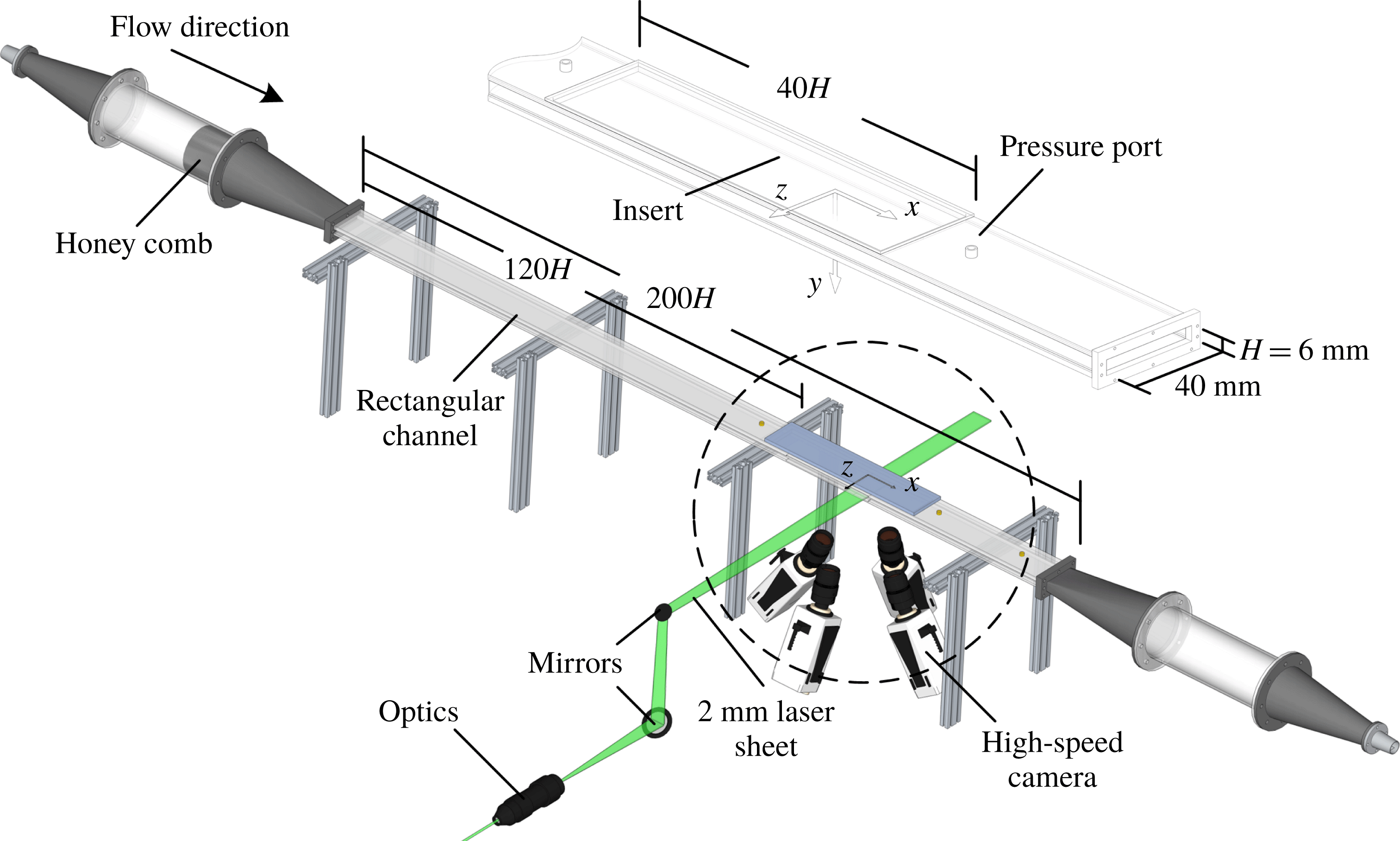
The experiments were conducted in a closed-circuit turbulent channel flow as shown in the schematic of figure 1. The test section had a rectangular cross-section with a height of $H=6~\text{mm}$ , width of $W=40~\text{mm}$ and total length of $1.2~\text{m}~(200H)$ . The aspect ratio $(W/H)$ of the channel cross-section was 6.7. This aspect ratio is close to the minimum recommended aspect ratio of 7 by Dean (Reference Dean1978) to maintain a two-dimensional (2-D) flow in the centre of the channel. The investigation of Vinuesa et al. (Reference Vinuesa, Noorani, Lozano-Durán, Khoury, Schlatter, Fischer and Nagib2014) also showed a negligible effect $({\sim}1\,\%)$ on centreline Reynolds stresses for a channel with an aspect ratio of 7. The top and bottom walls of the channel were made of transparent acrylic, while the sidewalls were made of glass. The coordinate system in the streamwise, wall-normal and spanwise directions is indicated with $x,y$ and $z$ as displayed in figure 1. The settling chamber upstream of the test section had a diameter of 82.5 mm and includes a honeycomb structure to break down the large eddies. The chamber was connected to the test section through a 3-D contraction, which was manufactured by 3-D printing and coated with epoxy. The contraction ratio with respect to the diameter of the chamber was $14:1$ in the $y$ -direction and $2:1$ in the $z$ -direction. The loop was equipped with a centrifugal pump controlled by a variable frequency driver (VFD). An electromagnetic flow meter (FLR6305D, Omega Engineering Inc., USA) was used to monitor the mass flow rate. A proportional-integral-derivative (PID) controller was developed with commercial software (LabView 2016, National Instruments) to control the flow rate. The PID controller communicated with the VFD to control the pump revolutions per minute through an input/output card (NI USB-6001, National Instruments).

Figure 1.

Schematic of the experimental set-up showing the rectangular channel, the camera arrangement and the illumination path for the 3D-PTV experiment. The inset shows a closer view of the test section and the replaceable insert to mount the SHS.

The pressure difference $(\text{d}P)$ over the test surface was monitored using a pressure transducer (P15, Validyne) with a 0.2 psi diaphragm. The transducer was connected to two pressure ports upstream and downstream of the test surface with a distance of 276 mm $(46H)$ . The uncertainty of the pressure measurement was approximately 2 % based on several repeated measurements over the smooth surface. The absolute pressure inside the loop was measured by another pressure transducer (Validyne 0.5 psi diaphragm) and maintained below the atmospheric pressure at 97 kPa. The pressure-drop measurement over the current SHS showed negligible DR when the test-section pressure was equal to or larger than the atmospheric pressure. As observed in the previous experiments of Lei et al. (Reference Lei, Li, Shi and Chen2009), Ling et al. (Reference Ling, Srinivasan, Golovin, McKinley, Tuteja and Katz2016) and Gose et al. (Reference Gose, Golovin, Boban, Mabry, Tuteja, Perlin and Ceccio2018), high pressure can push the air layer into the cavities of the SHS and expose the peaks of the roughness elements to the turbulent flow, reducing the DR performance of the SHS. Ling et al. (Reference Ling, Srinivasan, Golovin, McKinley, Tuteja and Katz2016) carried out experiments over an SHS at two different hydrostatic pressures (98 kPa and 122 kPa). They concluded that the air layer over the SHS is compressed inside the roughness elements at the higher pressure while it is maintained at the lower pressure. Recently, the shadowgraphy particle tracking velocimetry measurement of Reholon & Ghaemi (Reference Reholon and Ghaemi2018) was carried out at atmospheric pressure on a body of revolution sprayed with a superhydrophobic coating. They showed that the air layer over the SHS at the tested hydrostatic pressure was relatively flat and covered all the roughness elements except for the large roughness peaks which are exposed to the flow.

The experiments were operated at a constant flow rate with a bulk velocity of $U_{b}=0.93~\text{m}~\text{s}^{-1}$ , defined as the average velocity over the cross-section. The Reynolds number is $Re_{b}=7000$ , defined as $Re_{b}=U_{b}H/\unicode[STIX]{x1D708}$ , with $\unicode[STIX]{x1D708}$ denoting the kinematic viscosity equal to $8.02\times 10^{-7}~\text{m}^{2}~\text{s}^{-1}$ . The friction velocity over the no-slip smooth surface is $u_{\unicode[STIX]{x1D70F}0}=0.060~\text{m}~\text{s}^{-1}$ and the wall unit is $\unicode[STIX]{x1D706}_{0}=13.3~\unicode[STIX]{x03BC}\text{m}$ , based on the wall-normal gradient of mean velocity in the linear viscous sublayer as described in § 3.1. The estimation also agrees with the inner scaling obtained from Clauser’s method using the logarithmic law of the turbulent boundary layer (Clauser Reference Clauser1956). The friction Reynolds number is $Re_{\unicode[STIX]{x1D70F}}=225$ , defined as $Re_{\unicode[STIX]{x1D70F}}=u_{\unicode[STIX]{x1D70F}}H/(2\unicode[STIX]{x1D708})$ . 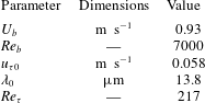The components of the instantaneous velocity vector are shown by $U$ , $V$ and $W$ , and the components of the fluctuating velocity by $u$ , $v$ and $w$ in the $x$ -, $y$ - and $z$ -directions, respectively. A summary of the channel flow parameters is listed in table 1.

2.2 Superhydrophobic surface

An SHS with a random texture was coated on the insert module using a commercial spray coating (Rust-Oleum NeverWet). This module has dimensions of 240 mm $(40H)$ and 40 mm in the $x$ - and $z$ -directions and was installed flush with the top wall 720 mm $(120H)$ downstream from the channel entrance as seen in figure 1. This spray coating was used in previous experiments (Aljallis et al. Reference Aljallis, Sarshar, Datla, Sikka and Jon2013; Zhang et al. 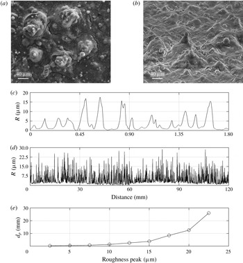Reference Zhang, Tian, Yao, Hao and Jiang2015; Vajdi Hokmabad & Ghaemi Reference Vajdi Hokmabad and Ghaemi2016; Abu Rowin, Hou & Ghaemi Reference Abu Rowin, Hou and Ghaemi2018) and is applied in two steps. First, a layer of base coat with no particles is sprayed to increase the adhesion of the surface. In the second step, a layer of particles is sprayed, which consists of particles with diameter from $5~\unicode[STIX]{x03BC}\text{m}$ up to $30~\unicode[STIX]{x03BC}\text{m}$ , as can be seen in the SEM images of figure 2. Contact-angle measurements were performed by characterizing the three-phase contact line using the Young–Laplace fitting method (Young Reference Young1805). Measurements were carried out using a droplet shape analyser (DSA-100 KRÜSS GmbH) by placing a $10~\unicode[STIX]{x03BC}\text{l}$ droplet at three locations over eight SHSs. The surfaces had an average contact angle of $152^{\circ }$ , with a standard deviation of $2.2^{\circ }$ . The contact-angle hysteresis was $2.8^{\circ }$ , with a standard deviation of $1.8^{\circ }$ , estimated as the difference between the advancing and receding contact angles. The roll-off angle over the current SHS was relatively small and equal to $1.4^{\circ }$ , with a standard deviation of  $0.6^{\circ }$ .

Table 1.

Summary of the parameters of the turbulent channel flow with smooth walls.

Figure 2.

SEM images with (a) top-down and (b) tilted views at $65^{\circ }$ of the randomly texture SHS. Samples of the profilometer measurement of microscale roughness of the SHS over (c) 1.8 mm and (d) 120 mm of the sample. (e) The mean distance between roughness peaks.

A step profiler (XP-300, Ambios Technology, USA) with $2.5~\unicode[STIX]{x03BC}\text{m}$ stylus tip radius and $30~\unicode[STIX]{x03BC}\text{m}~\text{s}^{-1}$ scanning speed was used to measure the variation of the SHS roughness heights as shown in figure 2(c). The measurement uncertainty was estimated to be approximately $0.1~\unicode[STIX]{x03BC}\text{m}$ based on measurement on a microscope slide (i.e. flat surface). The stylus force was set to 1 mg, since higher forces resulted in scratching the surface and peeling the hydrophobic coating. The surface roughness, $R$ , in figure 2(c) appears to have different peak heights up to approximately $20~\unicode[STIX]{x03BC}\text{m}$ . The root-mean-square of surface roughness $(R_{rms})$ was 4.9, with a standard deviation of $0.3~\unicode[STIX]{x03BC}\text{m}$ based on measurements at different locations on eight SHSs. The normalized roughness using the wall unit of the flow over the SHS is $k^{+}=R_{rms}/\unicode[STIX]{x1D706}=0.35$ , where $\unicode[STIX]{x1D706}=17~\unicode[STIX]{x03BC}\text{m}$ . The average texture width, $g$ , between the peaks with $R>3~\unicode[STIX]{x03BC}\text{m}$ is $85~\unicode[STIX]{x03BC}\text{m}$ , which is equivalent to $g^{+}=5.0\unicode[STIX]{x1D706}$ . The profilometer measurement over a longer distance of 120 mm is also shown in figure 2(d) to characterize the low-wavenumber features. The mean distance between roughness peaks ( $d_{p}$ ) which are larger than a prescribed threshold is illustrated in figure 2(d). As can be seen, $d_{p}$ increases with the increase of the roughness height and reaches up to a $d_{p}$ of 26 mm for the largest roughness peaks with $R=22~\unicode[STIX]{x03BC}\text{m}$ . The plastron visualization of Reholon & Ghaemi (Reference Reholon and Ghaemi2018), over an SHS with a similar structure under turbulent flow, has shown that at high DR $({>}15\,\%)$ a relatively flat air plastron covers the surface roughness. At lower DR, the surface elements are exposed to the liquid flow and a rough interface forms.

2.3 Time-resolved 3-D particle tracking velocimetry

Time-resolved 3D-PTV was used to measure the trajectory of tracer particles in a 3-D volume covering the inner layer over the test surfaces. The applied Lagrangian particle tracking technique is based on the shake-the-box (STB) method of Schanz et al. (Reference Schanz, Schröder, Gesemann and Wienek2013, Reference Schanz, Gesemann and Schröder2016) and carried out in DaVis 8.4 (LaVision GmbH). This method uses a combination of trajectory predictions and an image matching technique (shaking) based on the iterative particle reconstruction (IPR) technique of Wieneke (Reference Wieneke2012) to obtain an accurate estimation of particle position. The STB method can provide measurements with high spatial resolution in the vicinity of the wall $(y^{+}\sim 1)$ , as shown previously by Schröder et al. (Reference Schröder, Schanz, Geisler, Gesemann and Willert2015) and Novara et al. (Reference Novara, Schanz, Reuther, Kähler and Schröder2016).

The imaging system consisted of four high-speed Phantom v611 cameras with a complementary metal oxide semiconductor (CMOS) sensor of $1280~\text{pixel}\times 800~\text{pixel}$ . The CMOS sensor features $20~\unicode[STIX]{x03BC}\text{m}\times 20~\unicode[STIX]{x03BC}\text{m}$ pixels with 12-bit resolution. The cameras were arranged in a plus-like arrangement (Scarano Reference Scarano2012) as visualized in figure 1. The cameras were equipped with Scheimpflug adapters to align the depth of field with the laser sheet. Nikon 105 mm lenses with aperture settings of $f/22$ were used. The magnification and digital resolution of the imaging system were 0.56 and $35.5~\unicode[STIX]{x03BC}\text{m}~\text{pixel}^{-1}$ , respectively. The solid viewing angle between the wall-normal axis and the cameras was between $25^{\circ }$ and $30^{\circ }$ . The illumination was provided by a dual-head Nd:YLF laser (DM20-527, Photonics Industries) with $20~\text{mJ}~\text{pulse}^{-1}$ . Spherical and cylindrical lenses were used to form a collimated laser sheet. The lower edge of the laser sheet was cropped by a knife-edge filter, while the upper edge of the laser sheet was cropped by the channel wall to ensure a top-hat intensity profile starting from the wall surface. The cropping resulted in a final laser sheet thickness of 1.5 mm in the $y$ -direction and 21 mm in the $x$ -direction. The measurement volume was $21~\text{mm}\times 1.5~\text{mm}\times 21~\text{mm}~(1522\unicode[STIX]{x1D706}\times 108\unicode[STIX]{x1D706}\times 1522\unicode[STIX]{x1D706})$ , which is equivalent to $596~\text{pixel}\times 43~\text{pixel}\times 596~\text{pixel}$ in the $x$ -, $y$ - and $z$ -directions. The laser pulses and the four high-speed cameras were synchronized using a programmable timing unit (PTU X, LaVision GmbH) controlled by DaVis 8.2. Nine sets of 1610 single-frame images were recorded at a frequency of 4 kHz. At this recording frequency, the maximum particle displacement was approximately 11 pixels. One of the challenges for particle image velocimetry and PTV over SHSs is caused by the reflection of the laser light from the roughness elements and the shiny air plastron. Thus, the flow loop was seeded with $10~\unicode[STIX]{x03BC}\text{m}$ red fluorescent particles (polystyrene PS-FluoRed-Fi225) that emit light at a wavelength of 607 nm when illuminated with 530 nm green light. The experiments used a small particle image density of 0.003 particles per pixel (ppp) at $2{-}3~\text{particles}~\text{mm}^{-3}$ . This small particle image density is not a limitation of STB as the algorithm is capable of processing images with up to 0.075 ppp (Schanz et al. Reference Schanz, Gesemann and Schröder2016). In the current experiment, the smaller particle image density was chosen due to the large amount of monodisperse fluorescent particles required to seed ${\sim}40$  litres of water. As result, spatially uncorrelated data at low ppp were collected over a longer time to obtain statistical convergence. The band-pass filters (#1108573, LaVision) with wavelength limits of 545–800 nm were attached to each camera to record only the fluorescent emitted light.

A 2-D calibration target with 2 mm spaced holes was utilized for the initial calibration of the four cameras. The target was moved twice with 1 mm increments in the $y$ -direction by a micrometer traverse, resulting in three parallel planes. The mapping function between the image and the physical 3-D space was carried out using a pinhole model. Owing to small movements of the test section and a relatively large magnification, a large initial distortion of approximately 2–3 pixels was seen in the disparity map. The volume self-calibration (VSC) algorithm of Wieneke (Reference Wieneke2008) was applied to reduce the residual root-mean-square to approximately 0.02 pixels.

The minimum intensity of images was subtracted from each image, followed by normalization using the average image to increase the signal-to-noise ratio. The images were further improved by applying local intensity normalization over a window with a kernel of 10 pixels, and a Gaussian smoothing with a kernel of $3~\text{pixel}\times 3~\text{pixel}$ was used to avoid any peak locking (Kähler, Scharnowski & Cierpka Reference Kähler, Scharnowski and Cierpka2012). An optical transfer function (OTF) was obtained and used for every iterative particle reconstruction step and the shaking algorithm as described by Schanz et al. (Reference Schanz, Gesemann, Schröder, Wienek and Novara2012). We limited the largest particle shift between two successive image frames to 13 pixels and allowed a maximum triangulation error of 0.5 pixels. Particles closer than 1 pixel were eliminated to prevent any erroneous particle trajectories. The wall location was obtained using the minimum intensity of the ensemble of images, which includes a few surface glare points. The minimum image is reconstructed into a 3-D domain using the multiplicative algebraic reconstruction technique (MART) to obtain the 3-D location of the surface glares. The intensity of the reconstructed glare points is summed along the $x$ - and $z$ -directions and fitted with a Gaussian distribution to obtain the wall location with subpixel accuracy. The estimated uncertainty of the Gaussian fit is 0.1 pixel, equivalent to $0.26\unicode[STIX]{x1D706}_{0}$ .

To reduce the noise of particle trajectories and obtain the Lagrangian velocity and acceleration, polynomials with different orders and different kernel sizes can be fitted on the measured particle position. Gesemann et al. (Reference Gesemann, Huhn, Schanz and Schröder2016) applied a B-spline regression for noise reduction of STB data. Their regression method optimized the B-spline using a cost function assuming that the third derivative of particle position with respect to time ( jolt) has a white noise distribution. In the current investigation, we applied a simpler method using a second-order polynomial fitted to each component of particle location (i.e. $x$ , $y$ and $z$ ). The optimum polynomial kernel size is also based on the root-mean-square of acceleration $(a_{rms}^{+})$ as suggested by Voth et al. (Reference Voth, La Porta, Crawford, Alexander and Bodenschatz2002).

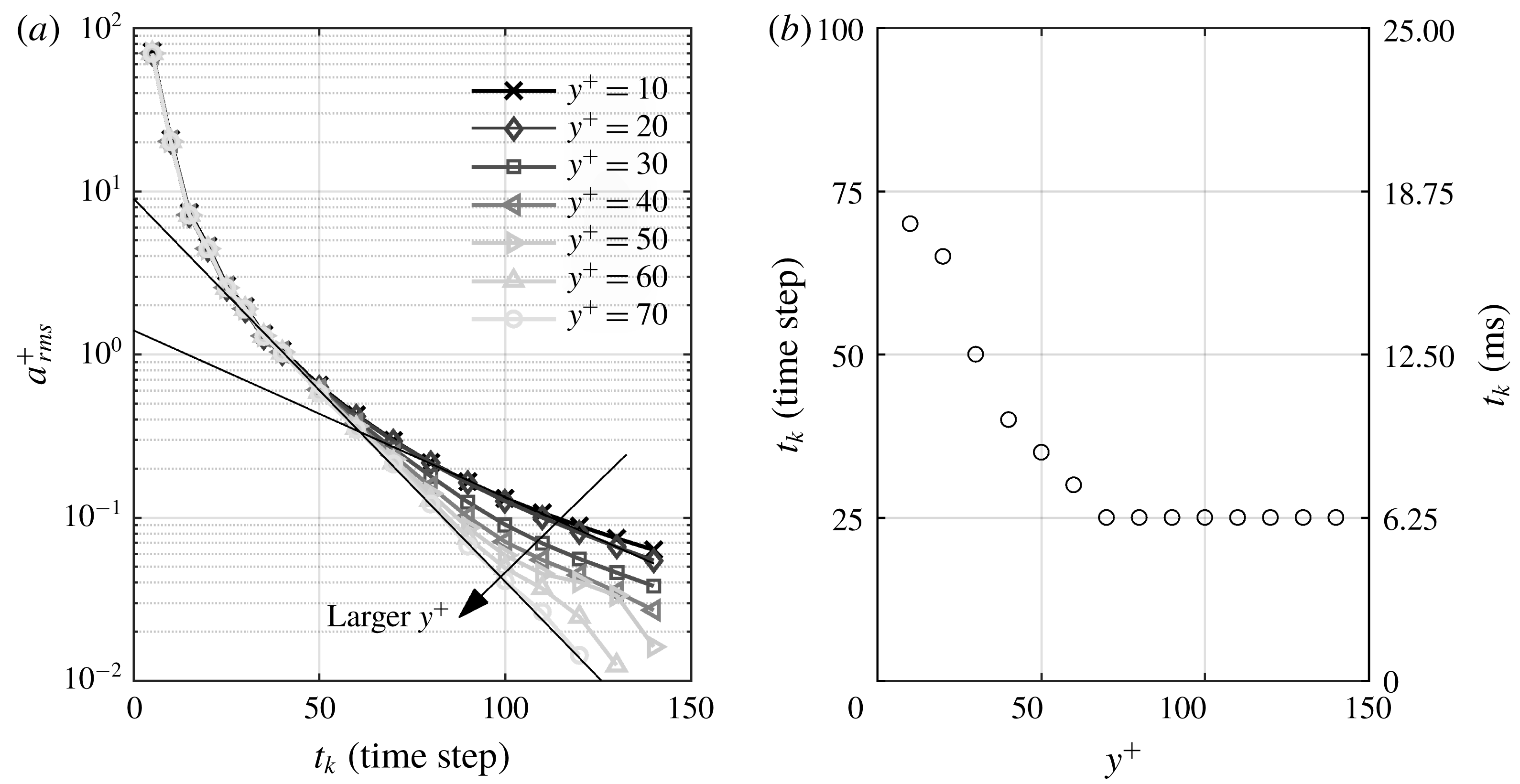
In figure 3(a), $a_{rms}^{+}$ is estimated at different wall-normal locations for a wide range of kernel sizes, shown in time steps of $\unicode[STIX]{x0394}t=250~\unicode[STIX]{x03BC}\text{s}$ . According to Voth et al. (Reference Voth, La Porta, Crawford, Alexander and Bodenschatz2002), an initial linear increase of $a_{rms}^{+}$ (in a semi-log presentation) should be observed when the kernel size reduces. As the kernel further reduces to a certain limit, $a_{rms}^{+}$ rapidly increases and deviates from the linear trend. The kernel size ( $t_{k}$ ) at which $a_{rms}^{+}$ deviates by 10 % from the linear trend is selected as the optimum kernel. For instance, in figure 3(a), $a_{rms}^{+}$ at $y^{+}=70$ follows a linear trend until $t_{k}$ reduces to 25 time steps. The optimum $t_{k}$ is estimated for different wall-normal locations and is presented in figure 3(b). The optimum size varies from $t_{k}=70$ time steps $(70\times 250~\unicode[STIX]{x03BC}\text{s})$ at $y^{+}=10$ to $t_{k}=25$ time steps $(25\times 250~\unicode[STIX]{x03BC}\text{s})$ at $y^{+}=70$ .

It is important to note that there is a steep wall-normal velocity gradient: the near-wall particles move by ${\sim}1$  pixel ( ${\sim}2u_{\unicode[STIX]{x1D70F}}$ at $y^{+}=2$ ) while the particles away from the wall move up to 11 pixels between two consecutive image frames $(\unicode[STIX]{x0394}t=250~\unicode[STIX]{x03BC}\text{s})$ . Therefore, more time steps are required for the near-wall particles to have a similar displacement (i.e. kernel length in pixels or millimetres) as the faster particles away from the wall.

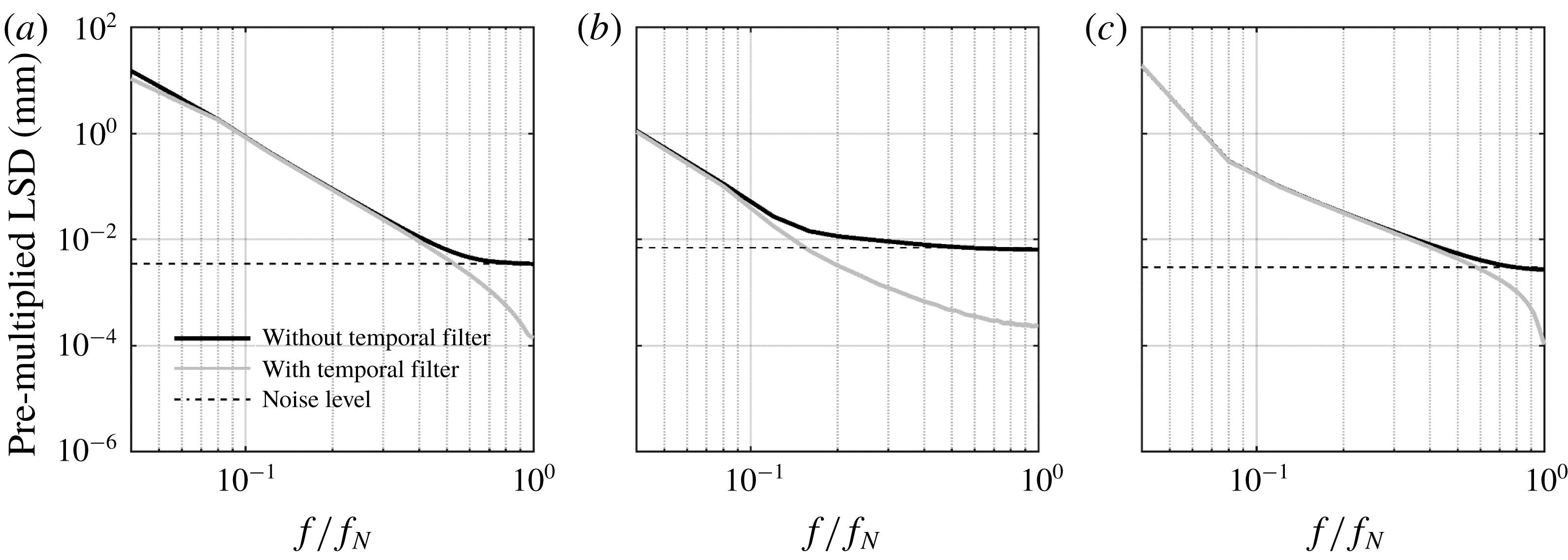
At each wall-normal location, the trajectories that are shorter than the optimum $t_{k}$ were discarded. The effect of the filter is evaluated using spectra of particle position (appendix B) and by comparing the measured Reynolds stresses over the smooth channel with the DNS of Gilbert & Kleiser (Reference Gilbert and Kleiser1991) and Rastegari & Akhavan (Reference Rastegari and Akhavan2015).

Figure 3.

(a) Variation of $a_{rms}^{+}$ with kernel size ( $t_{k}$ ) at different wall-normal locations. The solid straight black lines are fitted to $y^{+}=10$ and 70 data, showing that the $a_{rms}^{+}$ estimation deviates from the linear model at $t_{k}=70$ and 25, respectively. (b) The estimated optimum $t_{k}$ in time steps (left axis) and in milliseconds (right axis).

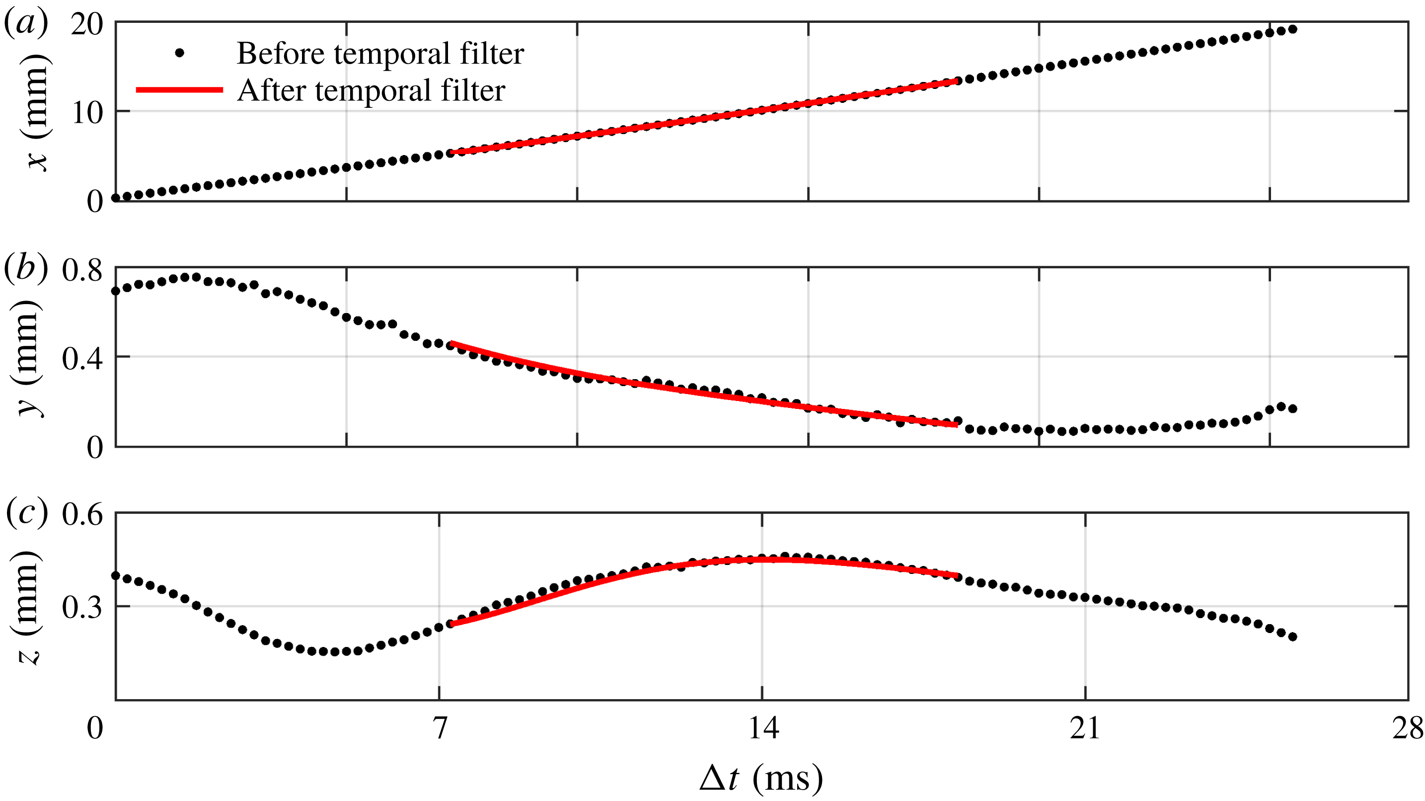
The $x$ -, $y$ - and $z$ -components of a trajectory before and after applying the second-order polynomial filter are shown in figure 4. The trajectory is at average wall-normal locations of $y=0.16~\text{mm}$ $(12\unicode[STIX]{x1D706})$ with $t_{k}$ of 60. As shown in figure 4(a), the raw trajectory in the $x$ -direction is smooth and the regression filter has a negligible effect. The trajectory in the $y$ -direction is relatively noisy in figure 4(b) as it is the out-of-plane motion for the cameras. However, the second-order polynomial filter can capture the motion and reduce the noise. The trajectory in the $z$ -direction in figure 4(c) has relatively low, negligible, noise compared with the $y$ -component. However, the second-order polynomial filter also captured the motion and reduced the noise. 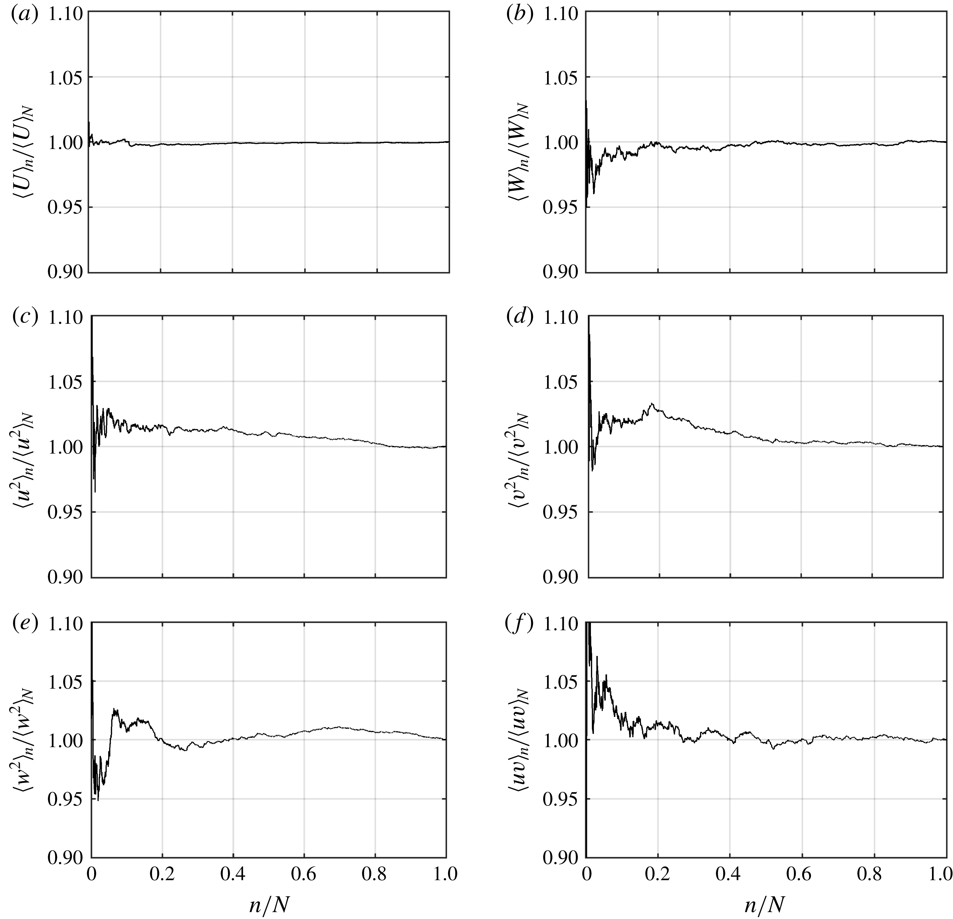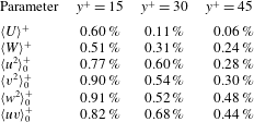The velocity of the particle is obtained from the coefficient of the second-order polynomial in the central part of the trajectory, where the full $t_{k}$ can be applied. This central part is shown with a solid line in figure 4. Evaluation of the random noise of the current 3D-PTV measurement for each component using the statistical convergence of the data is included in appendix A. The analysis shows that the random noise was minimal for the velocity profiles and limited to 0.60 % of the mean value at $y^{+}=15$ . However, the convergence analysis of Reynolds stresses showed a higher level of random noise, which reached up to 0.91 % of $\langle w^{2}\rangle$ at $y^{+}=15$ over the smooth surface.

Figure 4.

A particle trajectory before and after applying the regression in the (a) $x$ -, (b) $y$ - and (c) $z$ -directions. The trajectory is at an average wall-normal location of $y=0.16~\text{mm}$ .

3.1 Streamwise velocity

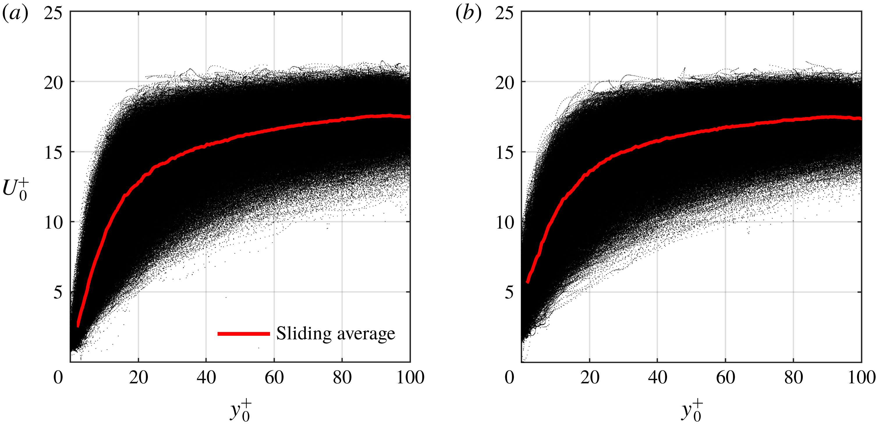
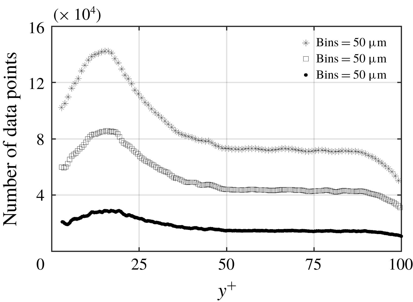
Scatter plots of the streamwise velocity of the particles over the smooth surface and SHS from 3D-PTV are shown in figures 5(a) and 5(b), respectively. The velocity over both surfaces is normalized using the inner scaling of the smooth surface ( $U_{0}^{+}=U/u_{\unicode[STIX]{x1D70F}0}$ ), and the plots cover the inner layer up to $y^{+}=100$ . The mean velocity profile is also shown using the solid lines by averaging the data over $10~\unicode[STIX]{x03BC}\text{m}~(0.72\unicode[STIX]{x1D706})$ bins with 75 % overlap. The mean velocity profile at $y^{+}<2.5$ is not shown due to its deviation from the expected linear viscous sublayer profile $\langle U\rangle ^{+}=y^{+}$ for the smooth surface. Therefore, $y^{+}=2.5$ is considered as the lower limit of the measurements. This limitation is imposed by the size of the fluorescent tracer particles $(d=10~\unicode[STIX]{x03BC}\text{m}=0.72\unicode[STIX]{x1D706})$ and lack of data at $y^{+}<2.5$ .

As shown in figure 5(a), there are a large number of particles with small $U_{0}^{+}~({<}2.5)$ in the immediate vicinity of the smooth wall, indicating the no-slip boundary condition. However, particles with larger $U_{0}^{+}$ varying from 2 to 8 $(0.12{-}0.48~\text{m}~\text{s}^{-1})$ are observed at the lowest wall-normal limit of the measurement in figure 5(b). The larger streamwise velocity at $y^{+}=2.5$ indicates the presence of a streamwise slip velocity at the SHS. The larger scatter of the instantaneous streamwise velocity in the vicinity of the SHS also agrees with the 2D-PTV of Abu Rowin et al. (Reference Abu Rowin, Hou and Ghaemi2017) over an SHS at $Re_{\unicode[STIX]{x1D70F}}=140$ .

Figure 5.

Streamwise velocity of the individual tracers over (a) smooth surface and (b) SHS. The data are normalized using inner variables of the smooth surface.

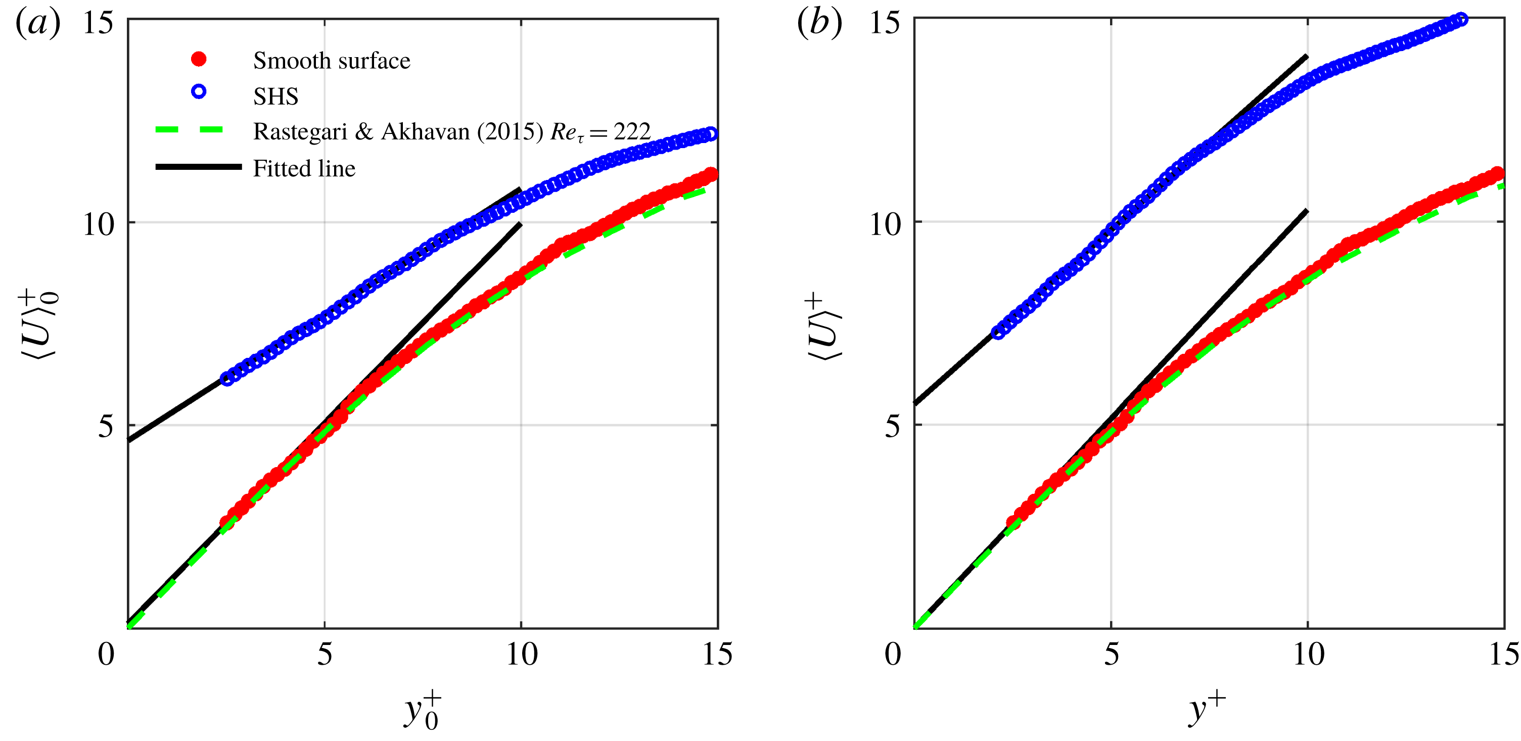
The mean streamwise velocities at $y^{+}<15$ over the smooth surface and SHS are presented in figure 6. The inner variables over the smooth surface are estimated using the wall-normal gradient of $\langle U\rangle$ within $2.5<y^{+}<3.5$ . Figure 6(a) shows that the mean streamwise velocity over the smooth surface follows the law of the wall $(y^{+}=\langle U\rangle ^{+})$ in the linear viscous sublayer and the DNS of Rastegari & Akhavan (Reference Rastegari and Akhavan2015) over the smooth channel at $Re_{\unicode[STIX]{x1D70F}}=222$ . The extrapolation of the fitted line on the velocity profile of the smooth surface approaches zero at the wall. The values of $\langle U\rangle _{0}^{+}$ over the SHS are higher than those of $\langle U\rangle _{0}^{+}$ over the smooth surface near the wall region due to the streamwise slip velocity. Farther away from the wall, the mean velocity over the SHS becomes smaller than over the smooth surface; however, the outer layer is not shown for brevity. The numerical simulation of Min & Kim (Reference Min and Kim2004), the theoretical work of Fukagata et al. (Reference Fukagata, Kasagi and Koumoutsakos2006) and the measurements of Abu Rowin et al. (Reference Abu Rowin, Hou and Ghaemi2017) have also observed a larger near-wall velocity and a smaller velocity farther away from an SHS. The slip velocity over the SHS is estimated by extrapolation of a linear fit over the near-wall velocity within $2.5<y^{+}<3.5$ to $y^{+}=0$ as shown in figure 6(a). The estimated slip velocity is $U_{s0}^{+}=U_{s}/u_{\unicode[STIX]{x1D70F}0}\approx 4.54$  ( $U_{s}=0.27~\text{m}~\text{s}^{-1}$ ), which results in $U_{s}/U_{b}\approx 30\,\%$ . The repeatability of the measurement is confirmed by carrying out the STB measurements over two additional SHSs manufactured through a similar spray coating procedure. The measured $U_{s}$ over these two SHSs are 0.30 and $0.25~\text{m}~\text{s}^{-1}$ , showing $\pm 8\,\%$ variation. The slope of this line is also used to estimate the inner scaling over the SHS. The estimated friction velocity over the SHS is $u_{\unicode[STIX]{x1D70F}}=0.048~\text{m}~\text{s}^{-1}$ , which is reduced by 17 % with respect to the smooth surface. This corresponds to $Re_{\unicode[STIX]{x1D70F}}=180$ over the SHS. In figure 6(b), the velocities over the smooth surface and SHS are normalized by their corresponding inner scaling. The fitted line over the mean velocity of the SHS within $2.5<y^{+}<3.5$ follows $\langle U\rangle ^{+}=y^{+}+U_{s}^{+}$ . The slip velocity normalized as $U_{s}^{+}=U_{s}/u_{\unicode[STIX]{x1D70F}}$ is 5.76, and the slip length is $l_{s}\approx 96.5~\unicode[STIX]{x03BC}\text{m}~(5.91\unicode[STIX]{x1D706})$ .

Figure 6.

Mean velocity profiles normalized by the inner variables of the (a) smooth surface and (b) their corresponding inner variables. The mean values are obtained over bins of $10~\unicode[STIX]{x03BC}\text{m}~(0.72\unicode[STIX]{x1D706})$ with 75 % overlap in the $y$ -direction. The fitted lines over the data of $2.5<y^{+}<3.5$ are shown with black solid line. The DNS of Rastegari & Akhavan (Reference Rastegari and Akhavan2015) at $Re_{\unicode[STIX]{x1D70F}}=222$ is also shown for comparison.

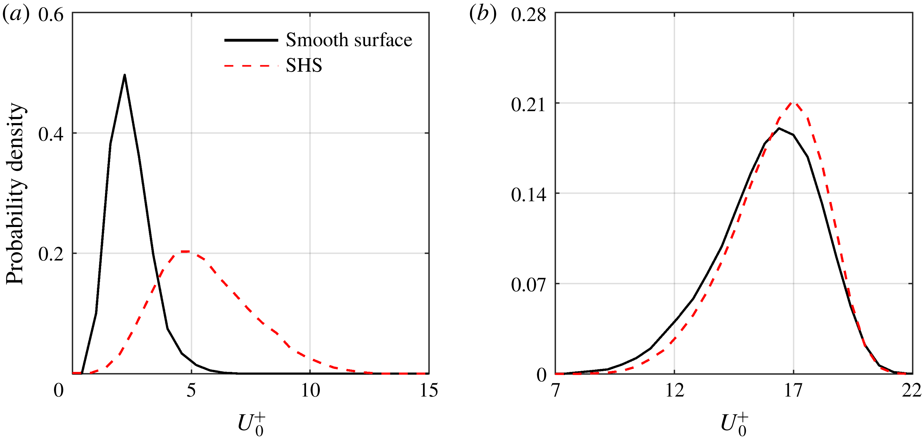
The probability density function (p.d.f.) of $U_{0}^{+}$ over the smooth surface and SHS in the immediate vicinity of the wall at $2.5<y^{+}<3.5$ is shown in figure 7(a). This p.d.f. shows that the SHS has shifted the streamwise velocity distribution towards larger velocities, with a broader distribution due to the streamwise slip velocity. Farther away from the wall at $45<y^{+}<46$ , the streamwise slip has a smaller influence on the p.d.f. of $U_{0}^{+}$ as shown in figure 7(b). Our investigation of different wall-normal locations within the log layer shows a similar trend: a slightly narrower p.d.f. for the SHS. The larger mean streamwise velocity and the wider p.d.f. for $2.5<y^{+}<3.5$ are consistent with the larger near-wall $\langle u^{2}\rangle$ observed in the numerical simulations of Min & Kim (Reference Min and Kim2004) and Rastegari & Akhavan (Reference Rastegari and Akhavan2015).

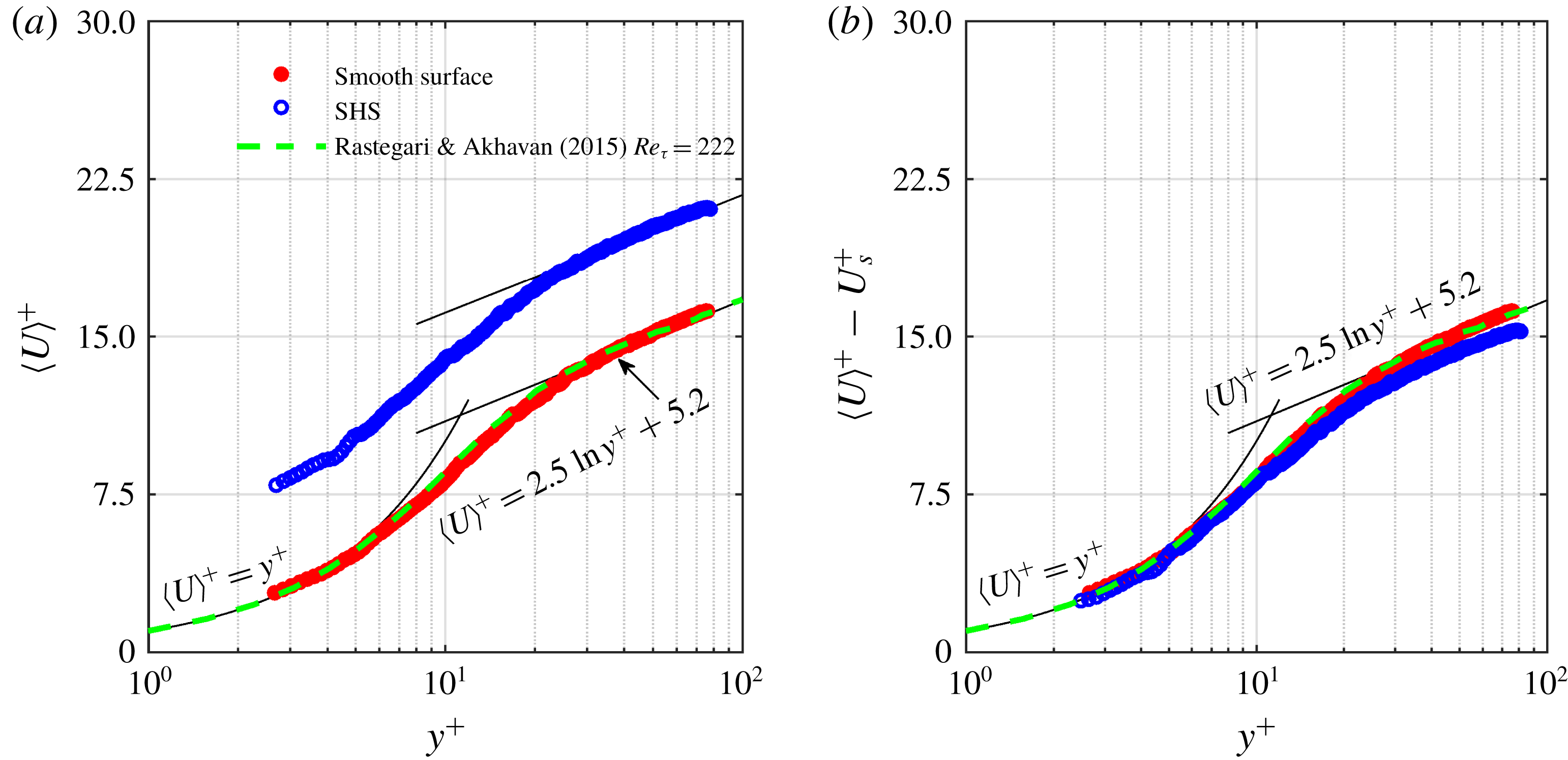
For the analysis of streamwise velocity over a wider wall-normal distance, semi-logarithmic presentations of $\langle U\rangle ^{+}$ over the smooth surface and SHS are plotted in figure 8(a), together with the DNS of Rastegari & Akhavan (Reference Rastegari and Akhavan2015). The data are normalized using the inner scaling of the corresponding surface obtained from the linear velocity gradient in figure 6(a). The law of the wall for the linear viscous sublayer as $\langle U\rangle ^{+}=y^{+}$ and the log law expressed as $\langle U\rangle ^{+}=(1/\unicode[STIX]{x1D705})\ln y^{+}+B$ are also shown with the von Kármán constant of $\unicode[STIX]{x1D705}=0.41$ and $B=5.2$ . The profile of the smooth surface agrees with the law of the wall and the log law, indicating a fully developed channel flow (Kim, Moin & Moser Reference Kim, Moin and Moser1987). The 3D-PTV measurements are also consistent with the DNS profile in the buffer layer range of $5<y^{+}<30$ . The $\langle U\rangle ^{+}$ of the SHS does not follow the standard log law and is shifted upwards due to the slip velocity. The upward shift of $\langle U\rangle ^{+}$ in the semi-logarithmic representation over an SHS has been observed in previous numerical simulations (e.g. Min & Kim Reference Min and Kim2004; Martell et al. Reference Martell, Rothstein and Perot2010) and experiments (Woolford et al. Reference Woolford, Princ, Maynes and Webb2009; Ling et al. Reference Ling, Srinivasan, Golovin, McKinley, Tuteja and Katz2016; Abu Rowin et al. Reference Abu Rowin, Hou and Ghaemi2017).

Figure 7.

Probability density functions of streamwise velocity over the smooth surface and SHS normalized by the inner variables of the smooth wall for data within (a)  $2.5<y^{+}<3.5$ and (b)  $45<y^{+}<46$ .

In figure 8(b), the slip velocity is subtracted from the mean velocity profile (i.e. $\langle U\rangle ^{+}-U_{s}^{+}$ ). As a result, the velocity profile over the SHS overlaps with the velocity profile over the smooth surface in the linear viscous sublayer for $y^{+}<3.5$ . In the buffer and log layers, the SHS velocity profile appears to have a slight downward shift. A similar downward shift was reported in the DNS of Min & Kim (Reference Min and Kim2004) when they imposed a slip velocity at the wall in both directions ( $l_{x}$ and $l_{z}$ ). Thus, the downward shift of the log law in figure 8(b) indicates the presence of both streamwise and spanwise slip over the current SHS.

3.2 Spanwise velocity

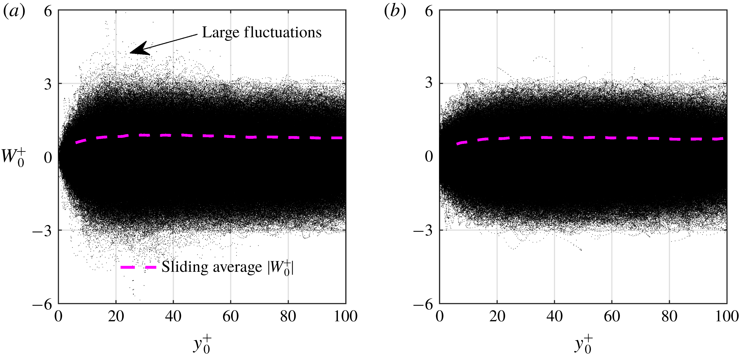
Scatter plots of the spanwise particle velocity over the smooth surface and SHS are presented in figures 9(a) and 9(b), respectively. The velocity over both surfaces is normalized using the inner scaling of the smooth surface. The mean of absolute spanwise velocity (i.e. $\langle W\rangle _{0}^{+}=\langle |W|\rangle /u_{\unicode[STIX]{x1D70F}0}$ ) is also presented with a solid line from an averaging process over windows of $30~\unicode[STIX]{x03BC}\text{m}~(2.2\unicode[STIX]{x1D706})$ with 75 % overlap in the $y$ -direction. The lower limit of the mean spanwise velocity is also set to $y^{+}=2.5$ , similar to the mean streamwise velocity. Owing to the no-slip condition, the spanwise velocity in the vicinity of the smooth surface is negligible in figure 9(a). In contrast, a large number of tracers with a finite spanwise velocity within $-0.8<W_{0}^{+}<0.8$ appear in the immediate vicinity of the SHS in figure 9(b). This large scatter of spanwise velocity confirms the presence of a spanwise slip velocity ( $W_{s}$ ). A narrower band of scattering in $W_{0}^{+}$ is observed away from the wall ( $y^{+}>20$ ) in figure 9(b) when compared with the smooth surface in figure 9(a). This will be further scrutinized by investigating profiles of $\langle w^{2}\rangle$ in the next section.

Figure 8.

(a) Semi-logarithmic plots of mean streamwise velocity normalized with the inner scaling of the corresponding surface $\langle U\rangle ^{+}$ . (b) Semi-logarithmic plots of $\langle U\rangle ^{+}-U_{s}^{+}$ . The DNS of Rastegari & Akhavan (Reference Rastegari and Akhavan2015) in a smooth channel at $Re_{\unicode[STIX]{x1D70F}}=222$ is also shown for comparison.

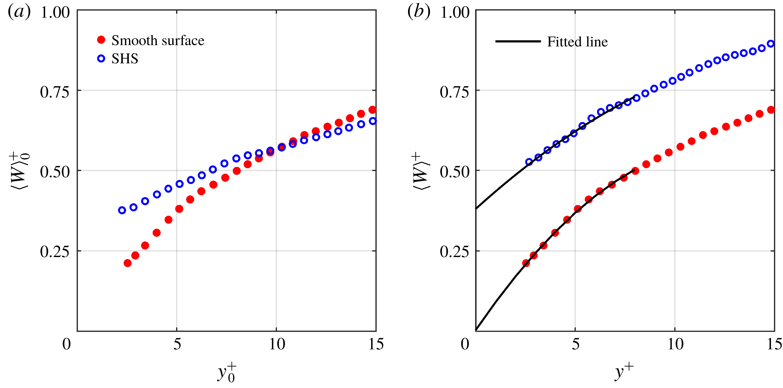
The profiles of $\langle W\rangle _{0}^{+}=\langle |W|\rangle /u_{\unicode[STIX]{x1D70F}0}$ over the smooth surface and SHS are shown in figure 10(a). The magnitude of $\langle W\rangle _{0}^{+}$ is much smaller than $\langle U_{0}\rangle ^{+};~\langle W\rangle _{0}^{+}$ is approximately $0.4u_{\unicode[STIX]{x1D70F}0}$ at $y^{+}=5$ while $\langle U\rangle _{0}^{+}$ is $5u_{\unicode[STIX]{x1D70F}0}$ at $y^{+}=5$ . The profile of $\langle W\rangle _{0}^{+}$ also does not follow a linear trend in the viscous sublayer. The values of $\langle W\rangle _{0}^{+}$ over the smooth surface tend towards a negligible velocity at the wall, confirming the no-slip boundary condition. The profile of $\langle W\rangle _{0}^{+}$ over the SHS is shifted upwards and approaches a finite value at the wall, indicating a slip velocity in the spanwise direction. Further away from the SHS at $y^{+}>10,~\langle W\rangle _{0}^{+}$ becomes smaller than that of the smooth surface. This trend is consistent with the streamwise velocity profile but the crossing point is closer to the wall due to the smaller spanwise slip velocity. The profiles of mean absolute spanwise velocity normalized with their corresponding inner scaling, $\langle W\rangle ^{+}=\langle |W|\rangle /u_{\unicode[STIX]{x1D70F}}$ , are shown in figure 10(b). It is observed in this figure that the variation of $\langle W\rangle _{0}^{+}$ can be described by a second-order polynomial. The extrapolation of the second-order polynomial within $2.5<y^{+}<7$ for the smooth surface to $y^{+}=0$ also results in zero $\langle W\rangle _{0}^{+}$ , which agrees with the no-slip boundary condition. Thus, the spanwise slip velocity and length over the SHS are estimated by applying a second-order polynomial to the data within $2.5<y^{+}<7$ . As displayed in figure 10(b), the extrapolation of this model results in a spanwise slip velocity of $0.38u_{\unicode[STIX]{x1D70F}}~(0.018~\text{m}~\text{s}^{-1})$ over the SHS, which corresponds to an effective spanwise slip length of $5.86\unicode[STIX]{x1D706}~(l_{z}\approx 95.8~\unicode[STIX]{x03BC}\text{m})$ .

Figure 9.

Spanwise velocity of the tracers over the (a) smooth surface and (b) SHS normalized by the inner scaling of the smooth surface. The dashed line shows the mean of the absolute value of spanwise velocity, $\langle |W|\rangle /u_{\unicode[STIX]{x1D70F}0}$ , obtained by averaging in $30~\unicode[STIX]{x03BC}\text{m}~(2.2\unicode[STIX]{x1D706})$ bins with 75 % overlap.

The magnitude of the slip length in the streamwise direction $(l_{x}=96.3~\unicode[STIX]{x03BC}\text{m}\approx 5.9\unicode[STIX]{x1D706})$ is comparable to the magnitude of the slip length in the spanwise direction $(l_{z}=95.8~\unicode[STIX]{x03BC}\text{m}\approx 5.9\unicode[STIX]{x1D706})$ . Therefore the slip boundary condition over the current randomly textured SHS with $k^{+}=0.35$ and $g^{+}=6$ is isotropic. The results confirm the DNS of Seo & Mani (Reference Seo and Mani2018), in which a randomly patterned SHS with texture width of $g^{+}=4.3$ was modelled assuming a homogenized isotropic slip length $(l_{x}=l_{z})$ . They observed that an SHS with a larger texture width $g^{+}=28.5$ cannot be modelled by an isotropic slip length model.

Figure 10.

Mean of the absolute spanwise velocity over the smooth surface and SHS obtained from averaging over $30~\unicode[STIX]{x03BC}\text{m}~(2.2\unicode[STIX]{x1D706})$ bins with 75 % overlap. The values are normalized by (a) the inner variables of the smooth surface and (b) the corresponding inner variables. Second-order polynomials with $\langle W\rangle ^{+}=-0.0035y^{+2}+0.0905y^{+}+0.0031$ and $\langle W\rangle ^{+}=-0.0015y^{+2}+0.0560y^{+}+0.3800$ are applied to the smooth surface and SHS profiles, respectively.

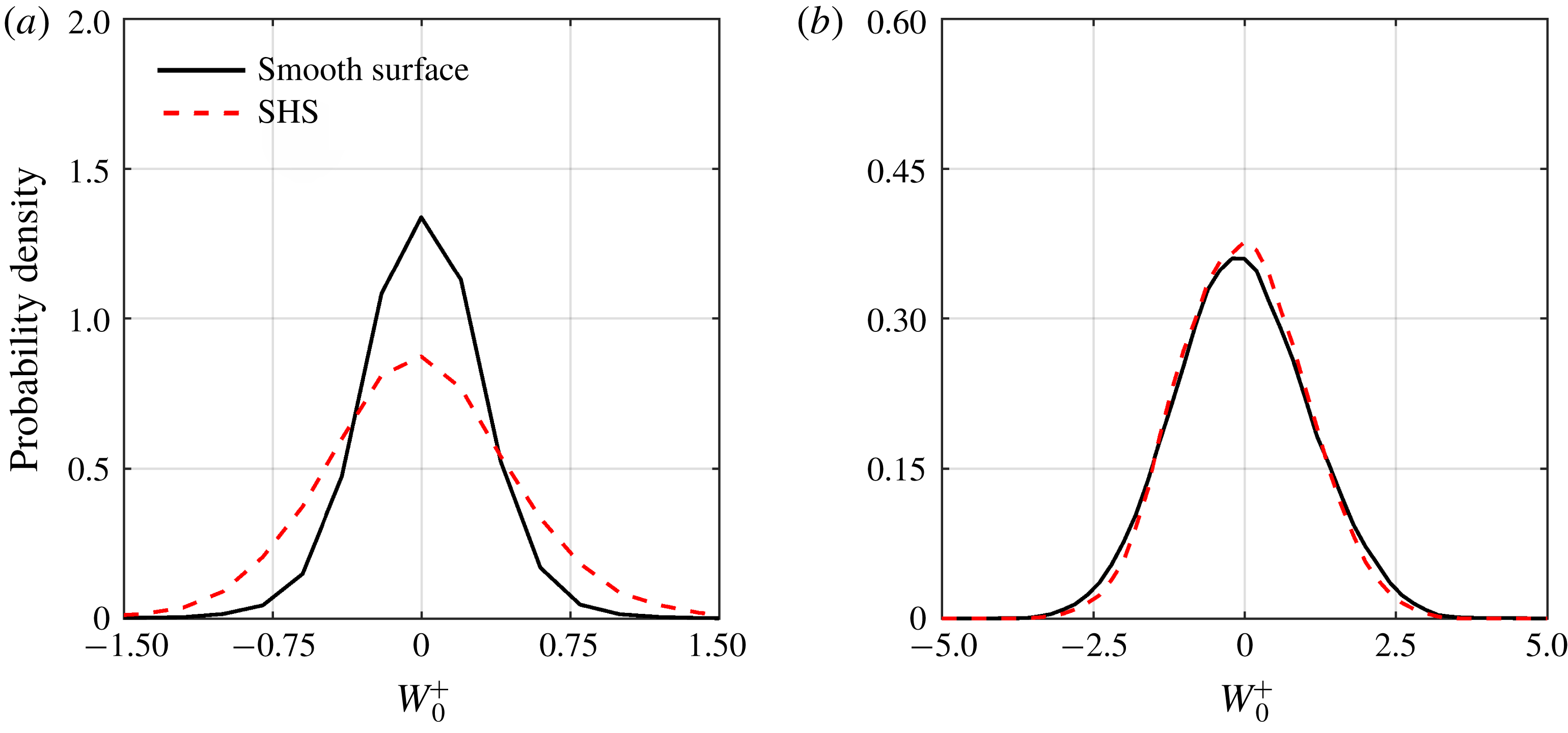
The p.d.f. of spanwise velocity over the smooth surface and the SHS for data within $2.5\leqslant y^{+}\leqslant 3.5$ and $45\leqslant y^{+}\leqslant 46$ are shown in figures 11(a) and 11(b), respectively. The SHS increases the probability of a large spanwise velocity and reduces the probability of a slow spanwise velocity within $2.5\leqslant y^{+}\leqslant 3.5$ . The effect reduces further away from the wall and the two p.d.f.s overlap in figure 11(b). The DNS of Min & Kim (Reference Min and Kim2004) also showed that an imposed $l_{z}$ at the wall (without $l_{x}$ ) increases $\langle w^{2}\rangle$ over an extended wall-normal distance; however, imposing both $l_{x}$ and $l_{z}$ results in a larger $\langle w^{2}\rangle$ only at a short wall-normal distance. The latter is due to an increase of turbulence by the spanwise slip.

Figure 11.

The probability density functions of spanwise velocity for velocity data within (a) $2.5<y^{+}<3.5$ and (b) $45<y^{+}<46$ .

3.3 Turbulence statistics

The profiles of the non-zero components of the Reynolds stress tensors over the smooth surface and SHS from 3D-PTV at $y^{+}<60$ are shown in figure 12. The Reynolds stresses in figure 12 are only shown at $y^{+}<60$ due to the lack of statistical convergence and larger error in Reynolds stresses close to the upper boundary of the 3D-PTV domain. The results from the DNS of Gilbert & Kleiser (Reference Gilbert and Kleiser1991) at an $Re_{\unicode[STIX]{x1D70F}}$ of 211 and Rastegari & Akhavan (Reference Rastegari and Akhavan2015) at an $Re_{\unicode[STIX]{x1D70F}}$ of 222 over the smooth surface are also shown for comparison. The two DNS data are also used to show the effect of a small change in $Re_{\unicode[STIX]{x1D70F}}$ since the smooth surface is at an $Re_{\unicode[STIX]{x1D70F}}$ of 217 and the SHS is at a lower $Re_{\unicode[STIX]{x1D70F}}$ of 180. Also, the DNS of Rastegari & Akhavan (Reference Rastegari and Akhavan2015) over an SHS modelled as an organized array of streamwise microgrooves with $U_{s}/U_{b}=0.32$ and a DR of 33 % is included in figure 12(b,d,f,h) for comparison. The SHS performance of the DNS is similar to the current investigation where $U_{s}/U_{b}=0.3$ and the DR is approximately 30 % (discussed in § 3.5). In addition, Reynolds stresses over an SHS with randomly distributed posts (with the same height) from the DNS of Seo & Mani (Reference Seo and Mani2018) are also included in figure 12(b,d,f,h). The simulated SHS of Seo & Mani (Reference Seo and Mani2018) has $U_{s0}^{+}=4.5$ , similar to the $U_{s0}^{+}=4.54$ of the current SHS. The averaging is carried out using windows of $50~\unicode[STIX]{x03BC}\text{m}~(3.8\unicode[STIX]{x1D706})$ with 75 % overlap in the $y$ -direction. The Reynolds stresses are normalized by the inner variables of the smooth surface (i.e. $\langle u_{i}u_{j}\rangle _{0}^{+}=\langle u_{i}u_{j}\rangle /u_{\unicode[STIX]{x1D70F}_{0}}^{2}$ ) in figure 12(a,c,g) at the left side and normalized using the inner variable of the corresponding surface (i.e. $\langle u_{i}u_{j}\rangle ^{+}=\langle u_{i}u_{j}\rangle /u_{\unicode[STIX]{x1D70F}}^{2}$ ) in figure 12(b,d,f,h) on the right side. When the Reynolds stresses of the SHS are normalized with the inner scaling of the smooth surface, it is possible to study their variation at a constant bulk flow rate without considering the change in friction velocity. Both normalizations have been applied in the literature.

The streamwise Reynolds stress of the smooth surface $\langle u^{2}\rangle _{0}^{+}$ in figure 12(a) follows the DNS profiles. There is a slight difference which is associated with the difference in $Re_{\unicode[STIX]{x1D70F}}$ and measurement noise. In the near-wall region of $y^{+}<12$ , $\langle u^{2}\rangle _{0}^{+}$ over the SHS is larger than over the smooth surface due to the streamwise slip. Away from the wall, $\langle u^{2}\rangle _{0}^{+}$ attenuates and becomes smaller than over the smooth surface. The closer distance of the $\langle u^{2}\rangle _{0}^{+}$ peak to the wall suggests a thinner inner layer over the SHS. The $\langle u^{2}\rangle _{0}^{+}$ peak is 16 % smaller than over the smooth surface and is shifted closer to the wall to $y^{+}=14$ . The DNS of Min & Kim (Reference Min and Kim2004) and Busse & Sandham (Reference Busse and Sandham2012) also reported an increase of $\langle u^{2}\rangle _{0}^{+}$ in the immediate vicinity of the wall and a reduction of $\langle u^{2}\rangle _{0}^{+}$ farther away from the wall when a finite $l_{x}$ was imposed. Min & Kim (Reference Min and Kim2004) also showed that the modulation of $\langle u^{2}\rangle _{0}^{+}$ became negligible when $l_{x}$ was reduced from $3.57\unicode[STIX]{x1D706}$ to $0.36\unicode[STIX]{x1D706}$ .

Figure 12.

The 3D-PTV measurement of (a,b) streamwise, (c,d) wall-normal, (f) spanwise and (g,h) shear Reynolds stresses over the smooth surface and SHS. The Reynolds stresses normalized by the inner variables of the smooth surface are denoted by $\langle u_{i}u_{j}\rangle _{0}^{+}$ in (a,c,e,g) and those normalized by the corresponding inner variables are indicated by $\langle u_{i}u_{j}\rangle ^{+}$ in (b,d,f,h).

When $\langle u^{2}\rangle$ of the SHS is normalized with its friction velocity in figure 12(b), $\langle u^{2}\rangle ^{+}$ of the SHS is larger than that of the smooth surface in the near-wall region and it slowly approaches $\langle u^{2}\rangle ^{+}$ of the smooth surface at approximately $y^{+}=45$ . A smaller $\langle u^{2}\rangle ^{+}$ is observed for the SHSs of Rastegari & Akhavan (Reference Rastegari and Akhavan2015) and Seo & Mani (Reference Seo and Mani2018) relative to the measurements over the SHS in figure 12(b). The $\langle u^{2}\rangle ^{+}$ gradually approaches the smooth surface with an increase of $y^{+}$ . The smaller $\langle u^{2}\rangle ^{+}$ of the DNS over the SHS compared with $\langle u^{2}\rangle ^{+}$ of the current investigation is associated with the uniform height of the roughness elements in simulations of Rastegari & Akhavan (Reference Rastegari and Akhavan2015) and Seo & Mani (Reference Seo and Mani2018). The roughness height of the random textured SHS in the current experiment varies spatially as seen in figure 2. However, both DNS and 3D-PTV measurements confirm a larger $\langle u^{2}\rangle ^{+}$ over the SHS relative to the smooth surface.

The wall-normal Reynolds stress, $\langle v^{2}\rangle _{0}^{+}$ , over the smooth surface in figure 12(c) also agrees with the DNS profiles. The profiles of $\langle v^{2}\rangle _{0}^{+}$ over the SHS and the smooth surface in figure 12(c) both start from zero at the wall as expected due to the non-permeable boundary condition. The overlap of $\langle v^{2}\rangle _{0}^{+}$ for the smooth surface and SHS at $y^{+}<10$ also suggests negligible oscillation and movement of the SHS plastron in the wall-normal direction. However, $\langle v^{2}\rangle _{0}^{+}$ of the SHS is smaller than the smooth surface in the inner layer, indicating smaller turbulence over the SHS. A similar trend is also seen in the DNS of Min & Kim (Reference Min and Kim2004) over a flat SHS and the measurement of Abu Rowin et al. (Reference Abu Rowin, Hou and Ghaemi2017) over an SHS with a roughness of $k^{+}=0.11$ . The DHM of Ling (Reference Ling2017) shows a larger $\langle v^{2}\rangle _{0}^{+}$ at the near-wall region of $y^{+}<10$ for SHSs with $k^{+}$ values as large as 0.89. The normalization based on the inner scaling of the corresponding surface results in larger values of $\langle v^{2}\rangle ^{+}$ over the SHS with respect to the smooth surface in figure 12(d). The $\langle v^{2}\rangle ^{+}$ of the DNS of Rastegari & Akhavan (Reference Rastegari and Akhavan2015) over the SHS in figure 12(d) is also larger than $\langle v^{2}\rangle ^{+}$ of the smooth surface within $10<y^{+}<30$ . The $\langle v^{2}\rangle ^{+}$ from Seo & Mani (Reference Seo and Mani2018) overlaps with $\langle v^{2}\rangle ^{+}$ of 3D-PTV.

The spanwise component of the normal Reynolds stress, $\langle w^{2}\rangle _{0}^{+}$ , over the smooth surface in figure 12(e) falls between the DNS profiles of Gilbert & Kleiser (Reference Gilbert and Kleiser1991) and Rastegari & Akhavan (Reference Rastegari and Akhavan2015). This is expected since the $Re_{\unicode[STIX]{x1D70F}}$ of the current measurements falls between the $Re_{\unicode[STIX]{x1D70F}}$ of Gilbert & Kleiser (Reference Gilbert and Kleiser1991) and Rastegari & Akhavan (Reference Rastegari and Akhavan2015). Figures 12(a) and 12(e) show that the SHS modifies $\langle w^{2}\rangle$ similarly to $\langle u^{2}\rangle$ . In figure 12(e), a larger $\langle w^{2}\rangle _{0}^{+}$ is observed over the SHS at $y^{+}<7$ due to the spanwise slip $(W_{s})$ , followed by a smaller $\langle w^{2}\rangle _{0}^{+}$ farther away from the wall. This is consistent with the DNS of Min & Kim (Reference Min and Kim2004) and Busse & Sandham (Reference Busse and Sandham2012). The crossing point for $\langle w^{2}\rangle _{0}^{+}$ is closer to the wall than for $\langle u^{2}\rangle _{0}^{+}$ due to a smaller magnitude of $W_{s}$ compared with $U_{s}$ . In figure 12(f), $\langle w^{2}\rangle ^{+}$ over the SHS is larger than over the smooth surface across the measurement domain. A similar trend is observed for $\langle w^{2}\rangle ^{+}$ of Rastegari & Akhavan (Reference Rastegari and Akhavan2015) and Seo & Mani (Reference Seo and Mani2018) over the SHS in figure 12(f).

The Reynolds shear stress in figure 12(g) overlaps with the DNS profiles. The $\langle uv\rangle _{0}^{+}$ of the SHS starts slightly larger than for the smooth surface at $y^{+}<8$ , while it is approximately 20 % smaller farther away from the wall. This trend was previously observed by Abu Rowin et al. (Reference Abu Rowin, Hou and Ghaemi2017) and Ling (Reference Ling2017). The level of increase in $\langle uv\rangle _{0}^{+}$ in the immediate vicinity of the SHS depends on the relative roughness of the SHS as discussed by Abu Rowin et al. (Reference Abu Rowin, Hou and Ghaemi2017). Ling et al. (Reference Ling, Srinivasan, Golovin, McKinley, Tuteja and Katz2016) noticed that $\langle uv\rangle _{0}^{+}$ over SHSs with large roughness $(k^{+}>1)$ is larger than over a smooth surface in both the inner and outer layer regions. In figure 12(h), $\langle uv\rangle ^{+}$ of the SHS is larger than over the smooth surface and gradually approaches the smooth surface with an increase of $y^{+}$ . The $\langle uv\rangle ^{+}$ profile from the DNS of Rastegari & Akhavan (Reference Rastegari and Akhavan2015) over the SHS in figure 12(h) follows the smooth surface. The low Reynolds shear stress of the DNS is associated with the assumed flatness of the SHS. The SHS simulated by Rastegari & Akhavan (Reference Rastegari and Akhavan2015) also results in a smaller $\langle uv\rangle ^{+}$ .

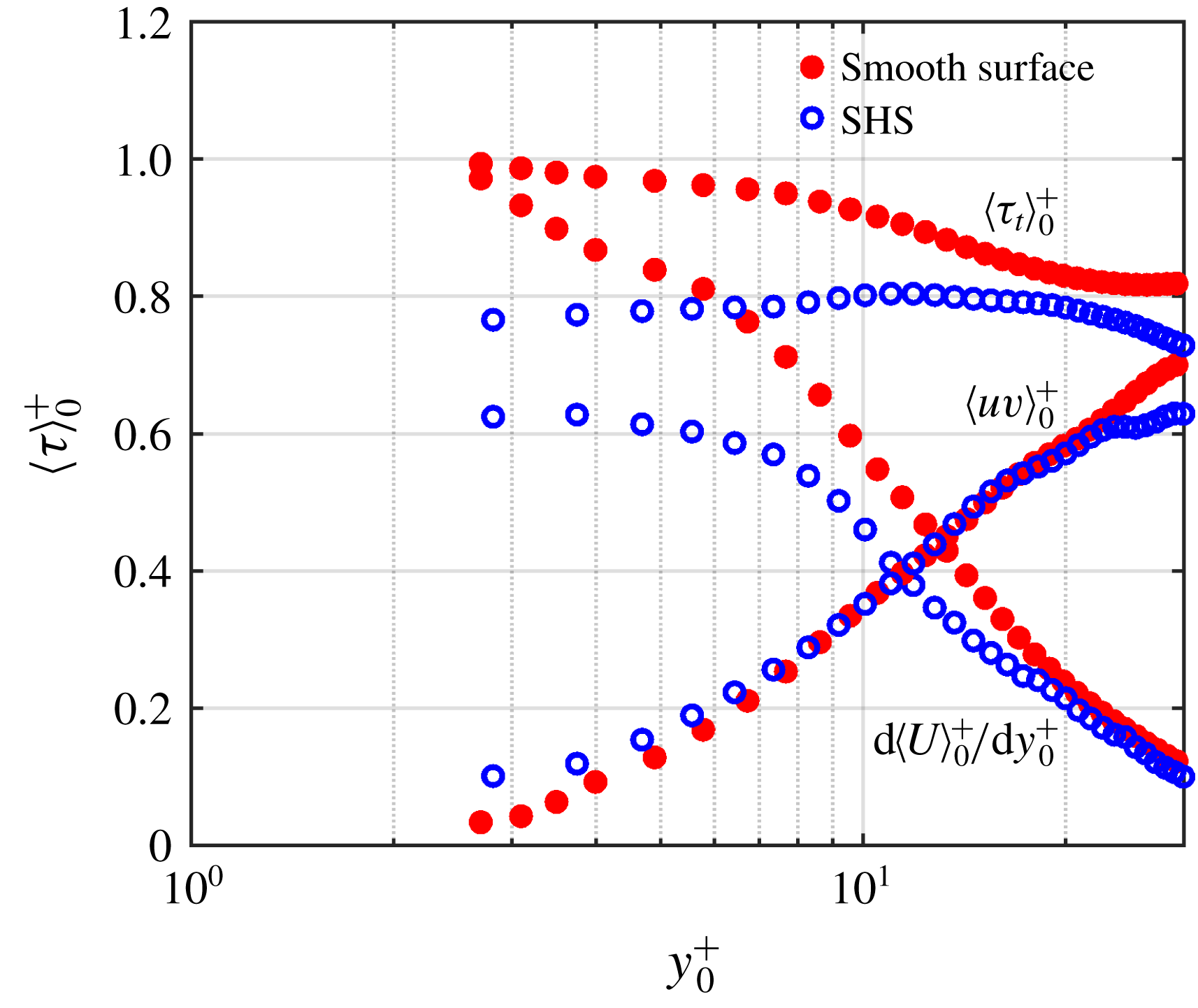
The distribution of viscous shear stress, $\unicode[STIX]{x1D70F}_{v0}^{+}=\text{d}\langle U\rangle _{0}^{+}/\text{d}y_{0}^{+}$ , Reynolds shear stress, $\unicode[STIX]{x1D70F}_{R0}^{+}=\langle uv\rangle _{0}^{+}$ , and the total shear stress, $\unicode[STIX]{x1D70F}_{t0}^{+}$ , over the smooth surface and the SHS are shown in figure 13. The shear stresses are normalized by the wall shear stress of the smooth surface $(\unicode[STIX]{x1D70F}_{w0}=\unicode[STIX]{x1D70C}u_{\unicode[STIX]{x1D70F}0}^{2})$ . Here $\unicode[STIX]{x1D70C}$ is the water density. It is observed that the viscous stress $\unicode[STIX]{x1D70F}_{v0}^{+}$ over the SHS is smaller than that over the smooth surface at $y^{+}<45$ due to the smaller wall-normal velocity gradient. Away from the wall, $\unicode[STIX]{x1D70F}_{v0}^{+}$ over the SHS overlaps with that over the smooth surface. The DHM measurement of Ling et al. (Reference Ling, Srinivasan, Golovin, McKinley, Tuteja and Katz2016) also reported a similar trend of smaller $\unicode[STIX]{x1D70F}_{v0}^{+}$ over the SHS compared with the smooth counterpart. They observed that $\unicode[STIX]{x1D70F}_{v0}^{+}$ of the SHS approaches $\unicode[STIX]{x1D70F}_{v0}^{+}$ of the smooth surface at $y^{+}=50$ . The Reynolds shear stress $\unicode[STIX]{x1D70F}_{R0}^{+}$ of the SHS is larger than that of the smooth surface at $y^{+}<10$ , due to the larger streamwise velocity fluctuations as seen in figure 12(a). Farther from the wall, $\unicode[STIX]{x1D70F}_{R0}^{+}$ of the smooth surface rapidly increases and becomes larger than $\unicode[STIX]{x1D70F}_{R0}^{+}$ of the SHS surface. The total shear stress $\unicode[STIX]{x1D70F}_{t0}^{+}$ over the SHS is smaller than that over the smooth surface within the measurement domain. As expected, the $\unicode[STIX]{x1D70F}_{t0}^{+}$ of the smooth surface approaches one at the wall. Over the SHS, $\unicode[STIX]{x1D70F}_{t0}^{+}$ increase with $y^{+}$ and reaches a local maximum at approximately $y^{+}=15$ . The increase of $\unicode[STIX]{x1D70F}_{t0}^{+}$ over the SHS in the near-wall region is also observed in the experiment of Ling et al. (Reference Ling, Srinivasan, Golovin, McKinley, Tuteja and Katz2016).

Figure 13.

Profiles of viscous shear stress ( $\unicode[STIX]{x1D70F}_{v0}^{+}$ ), Reynolds shear stress ( $\unicode[STIX]{x1D70F}_{R0}^{+}$ ) and total shear stress ( $\unicode[STIX]{x1D70F}_{t0}^{+}$ ) over the smooth surface and the SHS. The shear stresses are normalized by the wall shear stress of the smooth surface ( $\unicode[STIX]{x1D70F}_{w0}$ ).

3.4 The shear-free pattern

For an SHS with an organized pattern of cavities or grooves, the morphology of the shear-free pattern can be inferred based on the surface pattern. However, this is more complex for a random surface due to the large spectrum of roughness elements and sensitivity of the plastron morphology to environmental parameters such as pressure and dissolved air. The recent visualization of Reholon & Ghaemi (Reference Reholon and Ghaemi2018) showed the presence of a full plastron for high DR $({>}16\,\%)$ and isolated menisci of air, pinned between the tips and valleys of the roughness elements for lower DR $({<}8\,\%)$ over an SHS with a random texture. To investigate the shear-free pattern of the SHS, the streamwise velocity measured in the immediate vicinity of the wall is used here.

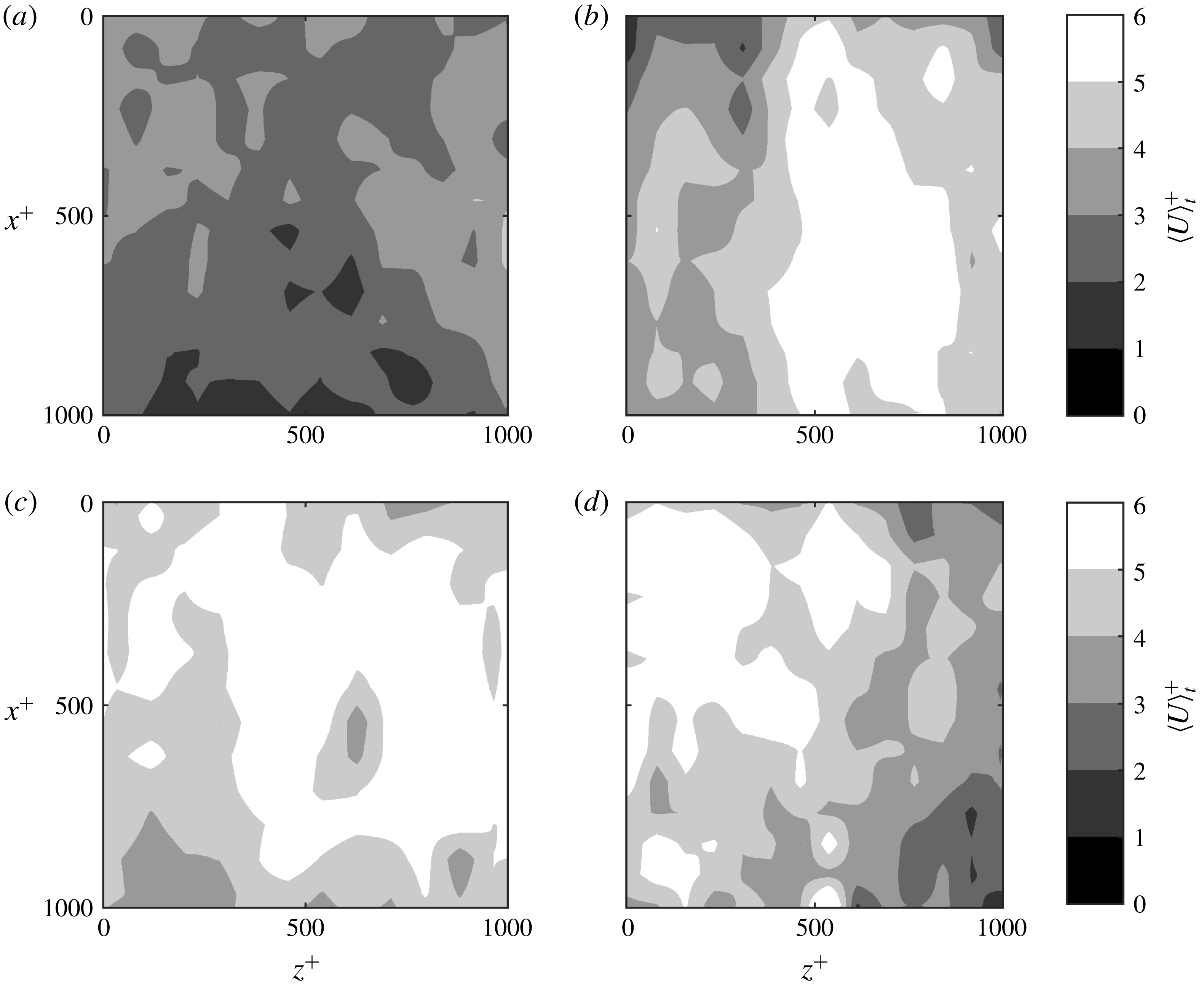
The spatial distribution of temporally averaged velocity $\langle U^{+}\rangle _{t}$ in an $x$ – $z$ plane with dimensions of $1000\unicode[STIX]{x1D706}\times 1000\unicode[STIX]{x1D706}~(13~\text{mm}\times 13~\text{mm})$ at $y^{+}=3$ over the smooth surface and SHS are shown in figure 14. The velocity data correspond to $2.5<y^{+}<3.5$ , binned into a grid of $75\unicode[STIX]{x1D706}\times 75\unicode[STIX]{x1D706}~(1~\text{mm}\times 1~\text{mm})$ windows in the $x$ – $z$ plane. The $\langle U^{+}\rangle _{t}$ distribution over the smooth surface in figure 14(a) shows a relatively uniform velocity distribution varying over $\langle U^{+}\rangle _{t}\approx 2{-}4$ . The variation is due to statistical convergence of the data when divided into the $1~\text{mm}\times 1~\text{mm}$ windows. The $\langle U^{+}\rangle _{t}$ contours over three separately fabricated SHSs are displayed in figure 14(b–d). The contours show higher streamwise velocity up to $\langle U^{+}\rangle _{t}\approx 6$ in patches as large as $800\unicode[STIX]{x1D706}\times 300\unicode[STIX]{x1D706}$  ( $13.6~\text{mm}\times 5.1~\text{mm}$ ) in the $x$ - and $z$ -directions, respectively. The high-speed patches indicate regions of substantial streamwise slip due to the thicker underneath air layer.

The DNS of Seo & Mani (Reference Seo and Mani2018) showed that randomly distributed posts with similar height can interrupt the shear-free regions. This interruption resulted in smaller shear-free areas, which in turn generated a smaller effective slip length compared with an organized counterpart with streamwise-aligned posts. In the current investigation, the variation of protrusion height allows the shear-free regions to extend between the peaks of the larger protrusions without interruption by the smaller roughness elements. The SEM images and the profilometer measurements in § 2.2 showed that the SHS roughness features with ${\sim}20~\unicode[STIX]{x03BC}\text{m}$ height occur at a mean distance of approximately 12 mm, similar to the streamwise length of the shear-free regions (see figure 14 a). This shows that the smaller peaks ( $R<20~\unicode[STIX]{x03BC}\text{m}$ ) do not disrupt the shear-free regions; the trapped air bubbles form a larger plastron pinned between the highest peaks. This is consistent with the DNS of Alame & Mahesh (Reference Alame and Mahesh2018) over a more realistic SHS with a random texture based on a 3-D scan of an SHS. They numerically showed that a thicker air layer can generate larger shear-free regions since small roughness elements are covered with the air plastron.

3.5 Drag estimation

In this section, the DR is estimated using several techniques, including pressure-drop measurements, estimation of wall-shear stress, the logarithmic law and the formulation of Rastegari & Akhavan (Reference Rastegari and Akhavan2015). The results are used to evaluate the analytical estimation of DR by Fukagata et al. (Reference Fukagata, Kasagi and Koumoutsakos2006), which explicitly includes the streamwise and spanwise slip lengths ( $l_{x}$ and $l_{z}$ ).

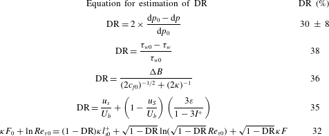
Drag reduction from pressure-drop measurement is expressed as $(\text{d}p_{0}-\text{d}p)/\text{d}p_{0}$ , where $\text{d}p_{0}$ is the pressure drop along the smooth surface and $\text{d}p$ is the pressure drop along the SHS. Although this method is straightforward, it is subject to relatively large uncertainties due to the small pressure drop ( ${\sim}700~\text{Pa}$ ) along the streamwise length of the SHS (240 mm) and partial coverage of the inner surface of the channel by the SHS coating. As previously discussed, the SHS is installed only at the top wall of the channel; however, the measured pressure drop is due to skin friction on the whole interior of the channel. Therefore, the DR by the SHS is estimated as $DR=2\times (\text{d}p_{0}-\text{d}p)/\text{d}p_{0}=30\,\%$ , where following Gose et al. (Reference Gose, Golovin, Boban, Mabry, Tuteja, Perlin and Ceccio2018) a factor of $2\times$ is applied due to partial coverage of the channel interior. Based on the error propagation theory (Hughes & Hase Reference Hughes and Hase2010) and the 2 % uncertainty in pressure-drop measurement, the uncertainty of the estimated DR is $\pm 8\,\%$ . To check the repeatability of DR, pressure-drop measurements were performed over two additional SHSs, showing 34 and 30 % DR.

Figure 14.

Mean velocity distribution over an $x$ – $z$ plane for (a) smooth surface and (b,c,d) three sample SHSs. The velocity is averaged within $2.5<y^{+}<3.5$ and a grid with $75\unicode[STIX]{x1D706}_{0}\times 75\unicode[STIX]{x1D706}_{0}$ windows is considered to generate the contours.

Ling et al. (Reference Ling, Srinivasan, Golovin, McKinley, Tuteja and Katz2016) estimated the DR over an SHS from direct measurement of wall shear stress ( $\unicode[STIX]{x1D70F}_{w}$ ) as a summation of viscous stress $(\unicode[STIX]{x1D70F}_{w}^{\unicode[STIX]{x1D707}}=\unicode[STIX]{x1D707}\unicode[STIX]{x2202}\langle U\rangle /\unicode[STIX]{x2202}y)$ and Reynolds shear stress ( $\unicode[STIX]{x1D70F}_{w}^{R}=-\unicode[STIX]{x1D70C}\langle uv\rangle$ ), where $\unicode[STIX]{x1D707}$ is the dynamic viscosity. As seen in figure 12(g), the Reynolds shear stress is expected to be negligible at $y^{+}=0$ over the current SHS due to its small roughness. Therefore, the DR is estimated here as $(\unicode[STIX]{x1D70F}_{w,0}^{\unicode[STIX]{x1D707}}-\unicode[STIX]{x1D70F}_{w}^{\unicode[STIX]{x1D707}})/\unicode[STIX]{x1D70F}_{w,0}^{\unicode[STIX]{x1D707}}$ , where the subscript $0$ refers to the wall shear stress over the smooth surface. The calculated DR is 38 % based on the wall shear stress estimated from the linear velocity gradient at $2.5<y^{+}<3.5$ .

The third method for estimating DR is based on a modification of the logarithmic law of the mean velocity profile as investigated by Min & Kim (Reference Min and Kim2004), Fukagata et al. (Reference Fukagata, Kasagi and Koumoutsakos2006), Busse & Sandham (Reference Busse and Sandham2012) and Rastegari & Akhavan (Reference Rastegari and Akhavan2019). For an SHS with DR, the von Kármán constant, $\unicode[STIX]{x1D705}$ , remains unchanged while the intercept of the logarithmic profile, $B$ , increases as seen in figure 8(a). Following the formulation of Bechert et al. (Reference Bechert, Brus, Hag, van der Hoeven and Hopp1997) in a study of riblet surfaces, DR can be obtained from

(3.1) $$\begin{eqnarray}\text{DR}=\frac{-\unicode[STIX]{x0394}B}{(2c_{f0})^{-1/2}+(2\unicode[STIX]{x1D705})^{-1}},\end{eqnarray}$$

where $\unicode[STIX]{x0394}B$ is the change of the intercept of the logarithmic profile between the smooth surface and SHS, and the skin-friction coefficient is defined as $c_{f}=\unicode[STIX]{x1D70F}_{w}/({\textstyle \frac{1}{2}}\unicode[STIX]{x1D70C}U_{b}^{2})$ . The estimated DR from (3.1) is 36 %. This method overestimates the DR by 4.0 % compared with the DR obtained from the reduction of the wall shear stress. The high DR from (3.1) can be associated with the negligible effect of the spanwise slip on the mean streamwise velocity profile away from the wall due to its small magnitude as shown by Min & Kim (Reference Min and Kim2004). In (3.1), $\unicode[STIX]{x0394}B$ is a function of surface structure, while $c_{f}$ depends on $Re$ (Rastegari & Akhavan Reference Rastegari and Akhavan2019).

Rastegari & Akhavan (Reference Rastegari and Akhavan2015) developed an expression to estimate DR over a wall with a slip-free boundary by decomposing the drag into a term due to slip velocity and another term due to modifications of the Reynolds shear stress based on the original formulation of Fukagata et al. (Reference Fukagata, Iwamoto and Kasagi2002). This decomposition of DR is given by

(3.2) $$\begin{eqnarray}\text{DR}=\frac{U_{s}}{U_{b}}+\left(1-\frac{u_{s}}{U_{b}}\right)\left(\frac{3\unicode[STIX]{x1D700}}{1-3I^{+}}\right).\end{eqnarray}$$

Here $\unicode[STIX]{x1D700}=I_{0}^{+}-I^{+}$ is the difference between the weighted integrals of $\langle uv\rangle ^{+}$ over the smooth surface and SHS, obtained from

(3.3) $$\begin{eqnarray}I^{+}=\int _{0}^{1}(1-\unicode[STIX]{x1D6FF})\langle uv^{+}\rangle \,\text{d}\unicode[STIX]{x1D6FF},\end{eqnarray}$$

where $\unicode[STIX]{x1D6FF}=2y/H$ is the normalized wall-normal coordinate. The integrals over the two surfaces in (3.3) were carried out within $2.5<y^{+}<90$  ( $0.01<\unicode[STIX]{x1D6FF}<0.4$ ). The limited range of integration does not affect the estimated DR due to the negligible value of $(1-\unicode[STIX]{x1D6FF})\langle uv\rangle ^{+}$ at $y^{+}<2.5$ and farther away from the wall at $y^{+}>90$ . The estimated DR from (3.2) is 35 %.

The expression of DR from the theoretical study of Fukagata et al. (Reference Fukagata, Kasagi and Koumoutsakos2006) includes both slip lengths ( $l_{x}$ and $l_{z}$ ) following

(3.4) $$\begin{eqnarray}\unicode[STIX]{x1D705}F_{0}+\ln Re_{\unicode[STIX]{x1D70F}0}=(1-\text{DR})\unicode[STIX]{x1D705}l_{x0}^{+}+\sqrt{1-\text{DR}}\ln (\sqrt{1-\text{DR}}\,Re_{\unicode[STIX]{x1D70F}0})+\sqrt{1-\text{DR}}\,\unicode[STIX]{x1D705}F.\end{eqnarray}$$

Here $F_{0}$ is obtained from $U_{b}/u_{\unicode[STIX]{x1D70F}}=\unicode[STIX]{x1D705}^{-1}\ln Re_{\unicode[STIX]{x1D70F}0}+F_{0}$ as expressed by Dean (Reference Dean1978) and is equal to 2.9. The parameter $F$ is a function of the non-dimensionalized spanwise slip length ( $l_{z}^{+}$ ). Fukagata et al. (Reference Fukagata, Kasagi and Koumoutsakos2006) estimated $F$ based on an exponential fit obtained from the numerical results of Min & Kim (Reference Min and Kim2004) as

(3.5) $$\begin{eqnarray}F=4\exp [-(0.14l_{z}^{+})^{0.7}]-0.8.\end{eqnarray}$$

This function results in $F\approx 0.75$ using the spanwise slip length obtained in § 3.2. The numerical solution of (3.4) results in a DR of 32 %, which underestimates DR by 3–6 % compared with the other techniques as shown in table 2. The low DR from (3.4) is associated with the estimated  $F$ from the DNS of Min & Kim (Reference Min and Kim2004), which assumes a flat boundary condition. The analysis shows that spanwise slip should be measured over a wider range of conditions, including $Re_{\unicode[STIX]{x1D70F}}$ and $k^{+}$ to develop more accurate analytical models for the estimation of drag over SHS.