1 Introduction
Calculating the hydrodynamic drag on a solid particle in an otherwise uniform stream of an incompressible Newtonian fluid is a fundamental problem in fluid mechanics. The drag is dependent on the particle shape and the Reynolds number
 $Re=\unicode[STIX]{x1D70C}UL/\unicode[STIX]{x1D707}$
, where
 $\unicode[STIX]{x1D70C}$
and
 $\unicode[STIX]{x1D707}$
are the density and viscosity of the fluid, respectively;
 $U$
is the speed of the imposed flow; and
 $L$
is the characteristic linear dimension of the particle. Exact results for the drag are available at zero Reynolds number for certain particle shapes (Happel & Brenner Reference Happel and Brenner1983). At non-zero
 $Re$
numerical or asymptotic methods must be applied to obtain approximate solutions to the Navier–Stokes equations and therefrom calculate the drag. Seminal works investigated the flow past an infinite circular cylinder and a sphere at small
 $Re$
via matched asymptotic expansions (Kaplun & Lagerstrom Reference Kaplun and Lagerstrom1957; Proudman & Pearson Reference Proudman and Pearson1957). Chester & Breach (Reference Chester and Breach1969) determined the drag on a sphere through terms of
 $O(Re^{3}\ln Re)$
. The force and torque on a particle of arbitrary shape that undergoes translation and rotation has been calculated through
 $O(Re^{2}\ln Re)$
by Cox (Reference Cox1965); remarkably, only the details of the Stokes flow (
 $Re=0$
) around the particle are needed to compute the force and torque to this order. Regrettably, the quantitative value of such asymptotic results is limited: in an appendix to Chester & Breach (Reference Chester and Breach1969), Proudman comments of their results that: ‘it is therefore particularly disappointing that the numerical ‘convergence’ of the expansion is so poor, and such as to limit its utility to the range
 $Re<1/2$
’. Here,
 $Re$
is defined with the radius of sphere serving as the length scale
 $L$
. Veysey & Goldenfeld (Reference Veysey and Goldenfeld2007) employed techniques from renormalization-group theory to derive perturbative approximations to the drag on a sphere and a cylinder, which are in qualitative agreement with numerical solutions and experiments up to
 $Re\approx 10$
. Roper & Brenner (Reference Roper and Brenner2009) constructed a non-perturbative approximation to the Navier–Stokes equations that yields quantitatively accurate predictions for the drag on a fore–aft symmetric body up to
 $Re=100$
. Their approximation is based on Carrier’s observation that the drag can be accurately calculated by a linearization of the Navier–Stokes equations in which: (i) the convective acceleration term
 $\boldsymbol{v}\boldsymbol{\cdot }\unicode[STIX]{x1D735}\boldsymbol{v}$
is replaced by
 $\boldsymbol{U}\boldsymbol{\cdot }\unicode[STIX]{x1D735}\boldsymbol{v}$
, where
 $\boldsymbol{v}$
is the fluid velocity, and
 $\boldsymbol{U}$
is the velocity of the uniform stream; and (ii) the viscosity
 $\unicode[STIX]{x1D707}$
is replaced by an effective viscosity that is a function of
 $Re$
(Carrier Reference Carrier1953).
In the present article, we consider the drag on an elongated particle at non-zero
 $Re$
. In Stokes flow it is well known that asymptotic approximations to the drag can be obtained via slender-body theory (Batchelor Reference Batchelor1970; Cox Reference Cox1970; Tillett Reference Tillett1970). These approximations take the form of a series in powers of
 $1/\text{ln}(1/\unicode[STIX]{x1D716})$
, where
 $\unicode[STIX]{x1D716}$
is the ratio of the characteristic width to length of the particle. It is less appreciated that slender-body theory can be utilized at non-zero
 $Re$
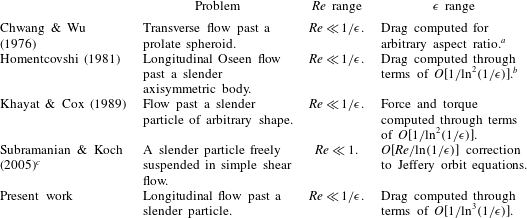
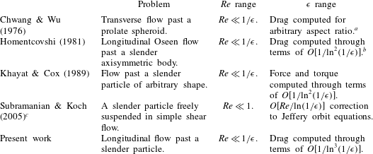
; indeed, there are only a handful of papers on this topic (table 1). The reason for its applicability is as follows: in the geometric ‘outer’ region, i.e. at distances from the particle surface on the order of the particle length, the leading-order disturbance to the uniform stream is asymptotically small in
 $\unicode[STIX]{x1D716}$
, scaling as
 $O[1/\text{ln}(1/\unicode[STIX]{x1D716})]$
. Therefore, this disturbance flow is governed by the linear Oseen equations; the particle is represented as a line distribution of the point-force solution to the Oseen equations, or ‘Oseenlet’. It is the fact that the leading-order outer problem is governed by a linear equation whose solution can be found with relative ease that enables the logarithmic expansion to proceed analytically. The same is true for slender-body analyses of scalar advection–diffusion equations (Romero Reference Romero1995; Schnitzer Reference Schnitzer2015; Relyea & Khair Reference Relyea and Khair2017). Recall that the Oseen equations are commonly encountered in the analysis of flow past a particle at small Reynolds number. Therein they describe the balance of vorticity advection (by the uniform stream) and diffusion at distances on the order of
 $L/Re$
, which is far from the particle surface. In the present case, the Oseen equations arise as a slender particle produces a disturbance that is asymptotically small in
 $\unicode[STIX]{x1D716}$
, even though the Reynolds number (based on the body length) need not be small.
Synopsis of papers on slender-body theory at non-zero
 $Re$
.
a
Khayat & Cox (Reference Khayat and Cox1989) point out that Chwang & Wu (Reference Chwang and Wu1976) erroneously assumed that the force per unit length on the spheroid is independent of the position along its centreline, which leads to an incorrect expression for the drag in the limit
 $\unicode[STIX]{x1D716}\rightarrow 0$
.
b
Homentcovshi (Reference Homentcovshi1981) presents an integral equation that can, in principle, be used to compute the drag to all logarithmic orders; however, the Oseen equations provide a systematic approximation to the drag in Navier–Stokes flow only through
 $O[1/\text{ln}^{2}(1/\unicode[STIX]{x1D716})]$
.
c
In subsequent work, these authors considered the dynamics of suspensions of slender particles at finite
 $Re$
(Shin, Subramanian & Koch Reference Shin, Subramanian and Koch2006, Reference Shin, Subramanian and Koch2009).
Khayat & Cox (Reference Khayat and Cox1989) used slender-body theory to derive expansions of the force and torque on a particle fixed in a uniform stream through terms of
 $O[1/\text{ln}^{2}(1/\unicode[STIX]{x1D716})]$
. These expansions are asymptotic provided
 $Re\ll O(1/\unicode[STIX]{x1D716})$
. They demonstrated that the inertial contribution to the force and torque is independent of the cross-sectional profile of the particle, which is surprising given one’s intuition (based on large
 $Re$
flows) that the drag on a body can be reduced by streamlining its profile. This finding provides the impetus for the present work, in which an expansion for the drag on an axisymmetric slender particle aligned with the uniform stream is calculated through
 $O[1/\text{ln}^{3}(1/\unicode[STIX]{x1D716})]$
. We find that the inertial contribution to the drag is dependent on the profile of the cross-section at this order. However, the drag is insensitive to the direction of travel of the particle. We compare the results of our asymptotic analysis to a numerical solution of the Navier–Stokes equations for the particular case of a prolate spheroid; good agreement is found.
In § 2 we present the equations governing the problem. In § 3 we perform the slender body analysis. The results of this analysis are discussed in § 4.
2 Governing equations
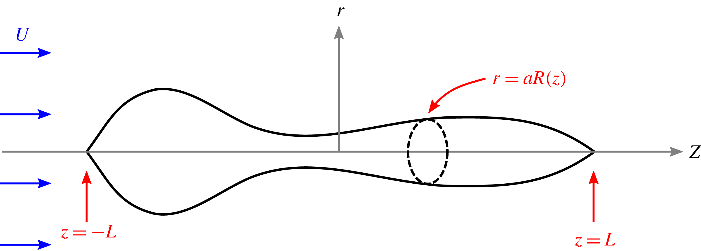
A rigid axisymmetric particle is held fixed in an incompressible Newtonian fluid. The fluid at large distances from the particle flows with a uniform velocity field directed along the axis of symmetry of the particle. The particle has a half-length
 $L$
and a characteristic cross-sectional radius
 $a$
, with
 $\unicode[STIX]{x1D716}=a/L\ll 1$
. Hence, the particle is slender. We adopt a cylindrical polar coordinate system
 $(r,\unicode[STIX]{x1D719},z)$
such that the particle surface is given by
 $$\begin{eqnarray}-L\leqslant z\leqslant L\quad \text{and}\quad r=aR(z),\end{eqnarray}$$
where
 $R(z)$
is a dimensionless shape function that vanishes at the endpoints,
 $z=\pm L$
, and varies on the length scale
 $L$
(figure 1). The steady, axisymmetric flow around the particle has a velocity field
 $$\begin{eqnarray}\boldsymbol{v}=u(r,z)\boldsymbol{e}_{r}+w(r,z)\boldsymbol{e}_{z},\end{eqnarray}$$
where
 $\boldsymbol{e}_{r}$
and
 $\boldsymbol{e}_{z}$
are unit vectors along the
 $r$
and
 $z$
axis, respectively. The fluid motion satisfies the steady Navier–Stokes equations
 $$\begin{eqnarray}\unicode[STIX]{x1D70C}\boldsymbol{v}\boldsymbol{\cdot }\unicode[STIX]{x1D735}\boldsymbol{v}=\unicode[STIX]{x1D707}\unicode[STIX]{x1D6FB}^{2}\boldsymbol{v}-\unicode[STIX]{x1D735}p,\quad \text{and}\quad \unicode[STIX]{x1D735}\boldsymbol{\cdot }\boldsymbol{v}=0,\end{eqnarray}$$
where
 $p$
is the dynamic pressure. The velocity field
 $\boldsymbol{v}\rightarrow U\boldsymbol{e}_{z}$
as
 $\sqrt{r^{2}+z^{2}}\rightarrow \infty$
. The fluid obeys the no-slip condition (
 $\boldsymbol{v}=0$
) on the surface of the particle. Our goal is to exploit the slenderness of the particle to yield an asymptotic approximation for the force,
 $\boldsymbol{F}$
, required to hold the particle fixed. This force is solely along the axis of symmetry of the particle; hence,
 $\boldsymbol{F}=-F\boldsymbol{e}_{z}$
, where
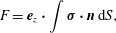 $$\begin{eqnarray}F=\boldsymbol{e}_{z}\boldsymbol{\cdot }\int \unicode[STIX]{x1D748}\boldsymbol{\cdot }\boldsymbol{n}\,\text{d}S,\end{eqnarray}$$
is the drag on the particle. In (2.4),
 $\boldsymbol{n}$
is the unit normal vector to the particle surface pointing into the fluid; the stress tensor
 $\unicode[STIX]{x1D748}=-p\unicode[STIX]{x1D644}+\unicode[STIX]{x1D707}[\unicode[STIX]{x1D735}\boldsymbol{v}+(\unicode[STIX]{x1D735}\boldsymbol{v})^{\dagger }]$
, where the superscript
 $\dagger$
denotes the transpose operation; and
 $\text{d}S$
is a differential area element on the particle surface.
Definition sketch of the problem set-up and cylindrical coordinate system.

3 Slender-body theory
We begin by making the problem dimensionless; let distance be normalized by
 $L$
, velocity normalized by
 $U$
and pressure and stress normalized by
 $\unicode[STIX]{x1D707}U/L$
. Henceforth, all variables and equations are dimensionless unless stated otherwise. The dimensionless Navier–Stokes equations are
 $$\begin{eqnarray}Re\boldsymbol{v}\boldsymbol{\cdot }\unicode[STIX]{x1D735}\boldsymbol{v}=\unicode[STIX]{x1D6FB}^{2}\boldsymbol{v}-\unicode[STIX]{x1D735}p,\quad \text{and}\quad \unicode[STIX]{x1D735}\boldsymbol{\cdot }\boldsymbol{v}=0,\end{eqnarray}$$
where
 $Re=\unicode[STIX]{x1D70C}UL/\unicode[STIX]{x1D707}$
is a Reynolds number based on the half-length of the particle. We stipulate that
 $\unicode[STIX]{x1D716}\ll 1$
; the restrictions that must be placed on the values of
 $Re$
will emerge in due course. Note that
 $Re=L/l$
, where
 $l=\unicode[STIX]{x1D707}/\unicode[STIX]{x1D70C}U$
is the inertial screening length, at which distance from the particle inertial and viscous forces are comparable. As usual in slender-body theory, the analysis of (3.1) is compartmentalized into geometric inner and outer regions, corresponding to
 $r\sim O(\unicode[STIX]{x1D716})$
and
 $r\sim O(1)$
, respectively. We proceed with an analysis of the inner region.
3.1 Inner region
Radial variations are on the dimensional scale of
 $1/a$
in the inner region, whereas axial variations are on the much longer scale of
 $1/L$
. Let
 $\unicode[STIX]{x1D70C}=r/\unicode[STIX]{x1D716}$
be a stretched (inner) coordinate with
 $\unicode[STIX]{x1D70C}$
fixed as
 $\unicode[STIX]{x1D716}\rightarrow 0$
. The inner region corresponds to
 $\unicode[STIX]{x1D70C}\sim O(1)$
and
 $-1\leqslant z\leqslant 1$
. Utilizing the continuity equation and the no-slip condition yields
 $u\sim O(\unicode[STIX]{x1D716}w)$
, where
 $w$
is at most
 $O(1)$
from the imposed uniform flow condition. Thus, the radial velocity is much smaller than the axial velocity in the inner region; in contrast, both are
 $O(1)$
in the outer region. From (3.1), the axial component of the momentum balance in the inner region is
 $$\begin{eqnarray}\unicode[STIX]{x1D716}^{2}Re\left(u\frac{\unicode[STIX]{x2202}w}{\unicode[STIX]{x2202}\unicode[STIX]{x1D70C}}+w\frac{\unicode[STIX]{x2202}w}{\unicode[STIX]{x2202}z}\right)=\frac{1}{\unicode[STIX]{x1D70C}}\frac{\unicode[STIX]{x2202}}{\unicode[STIX]{x2202}\unicode[STIX]{x1D70C}}\left(\unicode[STIX]{x1D70C}\frac{\unicode[STIX]{x2202}w}{\unicode[STIX]{x2202}\unicode[STIX]{x1D70C}}\right)+\unicode[STIX]{x1D716}^{2}\frac{\unicode[STIX]{x2202}^{2}w}{\unicode[STIX]{x2202}z^{2}}-\unicode[STIX]{x1D716}^{2}\frac{\unicode[STIX]{x2202}p}{\unicode[STIX]{x2202}z}.\end{eqnarray}$$
Inertial effects are negligible provided
 $Re\ll 1/\unicode[STIX]{x1D716}^{2}$
, which is a first restriction on the range of
 $Re$
for which our analysis is valid. The leading-order equation governing the axial velocity is simply
 $$\begin{eqnarray}\frac{1}{\unicode[STIX]{x1D70C}}\frac{\unicode[STIX]{x2202}}{\unicode[STIX]{x2202}\unicode[STIX]{x1D70C}}\left(\unicode[STIX]{x1D70C}\frac{\unicode[STIX]{x2202}w}{\unicode[STIX]{x2202}\unicode[STIX]{x1D70C}}\right)=0.\end{eqnarray}$$
The particle acts a source of vorticity due to the no-slip boundary condition; (3.3) states that for a slender object vorticity transport in the inner region is through radial diffusion. A similar situation occurs in the problem of forced convection heat and mass transfer from a slender body (Schnitzer Reference Schnitzer2015; Relyea & Khair Reference Relyea and Khair2017). Following Batchelor (Reference Batchelor1970), the solution to (3.3) is
 $$\begin{eqnarray}w=\frac{f(z;\unicode[STIX]{x1D716})}{2\unicode[STIX]{x03C0}}\ln \frac{\unicode[STIX]{x1D70C}}{R(z)},\end{eqnarray}$$
where
 $f(z;\unicode[STIX]{x1D716})$
is the axial force per unit length (normalized by
 $\unicode[STIX]{x1D707}U$
) on the particle. It is expected that
 $f(z;\unicode[STIX]{x1D716})$
is asymptotically small in
 $\unicode[STIX]{x1D716}$
, since the disturbance to the uniform stream (
 $w=1$
) should vanish as the particle thickness vanishes. In fact, rewriting (3.3) in terms of the outer radial coordinate yields
 $$\begin{eqnarray}w=\frac{f(z;\unicode[STIX]{x1D716})}{2\unicode[STIX]{x03C0}}\left[\ln \frac{r}{R(z)}+\ln \frac{1}{\unicode[STIX]{x1D716}}\right].\end{eqnarray}$$
Matching (3.5) to the uniform stream yields
 $f(z;\unicode[STIX]{x1D716})\sim 2\unicode[STIX]{x03C0}/\text{ln}(1/\unicode[STIX]{x1D716})$
to leading order. Hence, the net drag is
 $F\sim 4\unicode[STIX]{x03C0}/\text{ln}(1/\unicode[STIX]{x1D716})$
to leading order, which is independent of the cross-sectional profile
 $R(z)$
. This result is familiar from slender-body theory of Stokes flow (Taylor Reference Taylor1969; Batchelor Reference Batchelor1970; Cox Reference Cox1970; Tillett Reference Tillett1970); evidently, it also holds at non-zero Reynolds number, provided that inertial effects are negligible in the inner region. Moreover, at non-zero
 $Re$
the drag is
 $2F$
for uniform flow transverse to the axis of symmetry of the particle (Chwang & Wu Reference Chwang and Wu1976; Khayat & Cox Reference Khayat and Cox1989). Again, that the ratio of drags for flow in the transverse to axial directions equals 2 (to leading order in
 $\unicode[STIX]{x1D716}$
) is well known for Stokes flow; it is less appreciated that this result holds at non-zero
 $Re$
. The analysis above suggests the logarithmic expansion
 $$\begin{eqnarray}f(z;\unicode[STIX]{x1D716})=\frac{f_{0}(z)}{\ln (1/\unicode[STIX]{x1D716})}+\frac{f_{1}(z)}{\ln ^{2}(1/\unicode[STIX]{x1D716})}+\frac{f_{2}(z)}{\ln ^{3}(1/\unicode[STIX]{x1D716})}+\cdots \,,\end{eqnarray}$$
where
 $f_{0}=2\unicode[STIX]{x03C0}$
. The leading-order contribution to the drag is defined as
 $F_{0}=4\unicode[STIX]{x03C0}$
. Subsequent coefficients in this expansion are to be found by considering the velocity disturbance in the outer region. Before proceeding, note that the continuity equation and (3.5) yield the inner radial velocity
 $$\begin{eqnarray}u=\frac{\unicode[STIX]{x1D716}}{4\unicode[STIX]{x03C0}}\left[\frac{\text{d}f}{\text{d}z}r\left(\ln \frac{\unicode[STIX]{x1D70C}}{R}-\frac{1}{2}\right)-fr\frac{\text{d}\ln R}{\text{d}z}+\frac{R^{2}}{r}\left(\frac{1}{2}\frac{\text{d}f}{\text{d}z}+f\frac{\text{d}\ln R}{\text{d}z}\right)\right].\end{eqnarray}$$
Therefore, as argued above, the radial velocity is
 $O(\unicode[STIX]{x1D716})$
smaller than the axial velocity in the inner region. This implies that the matching of inner and outer velocity fields can be accomplished through consideration of the axial velocity component alone, provided that one does not wish to calculate terms in (3.6) that are exponentially small compared to
 $\ln (1/\unicode[STIX]{x1D716})$
.
3.2 Outer region: leading-order velocity disturbance
The outer region corresponds to
 $r$
fixed as
 $\unicode[STIX]{x1D716}\rightarrow 0$
. Here, the particle appears as a zero-width segment of length 2; the details of the cross-sectional profile enter through matching with the inner solution. Prompted by (3.6), the velocity and pressure fields in the outer region are expanded as
 $$\begin{eqnarray}\displaystyle & \displaystyle \boldsymbol{v}=\boldsymbol{v}_{0}+\frac{\boldsymbol{v}_{1}}{\ln (1/\unicode[STIX]{x1D716})}+\frac{\boldsymbol{v}_{2}}{\ln ^{2}(1/\unicode[STIX]{x1D716})}+\cdots \,, & \displaystyle\end{eqnarray}$$
 $$\begin{eqnarray}\displaystyle & \displaystyle p=\frac{p_{1}}{\ln (1/\unicode[STIX]{x1D716})}+\frac{p_{2}}{\ln ^{2}(1/\unicode[STIX]{x1D716})}+\cdots \,, & \displaystyle\end{eqnarray}$$
where
 $\boldsymbol{v}_{0}=\boldsymbol{e}_{z}$
is the uniform imposed flow, which is accompanied by a null pressure field. Inserting (3.8) and (3.9) into (3.1) shows that the leading-order velocity disturbance satisfies the Oseen equations
 $$\begin{eqnarray}Re\frac{\unicode[STIX]{x2202}\boldsymbol{v}_{1}}{\unicode[STIX]{x2202}z}=\unicode[STIX]{x1D6FB}^{2}\boldsymbol{v}_{1}-\unicode[STIX]{x1D735}p_{1},\quad \text{and}\quad \unicode[STIX]{x1D735}\boldsymbol{\cdot }\boldsymbol{v}_{1}=0,\end{eqnarray}$$
and
 $\boldsymbol{v}_{1}$
and
 $p_{1}$
attenuate at large distances. The solution to the Oseen equations due to a point force
 $\boldsymbol{g}\unicode[STIX]{x1D6FF}(\boldsymbol{x})=g\boldsymbol{e}_{z}\unicode[STIX]{x1D6FF}(\boldsymbol{x})$
at the origin, where
 $\boldsymbol{x}$
is the position vector and
 $\unicode[STIX]{x1D6FF}(\boldsymbol{x})$
is the Dirac delta function, yields the ‘Oseenlet’ velocity field
 $$\begin{eqnarray}\frac{\boldsymbol{g}}{4\unicode[STIX]{x03C0}|\boldsymbol{x}|}\text{e}^{(1/2)Re(z-|\boldsymbol{x}|)}+\frac{g}{4\unicode[STIX]{x03C0}Re}\unicode[STIX]{x1D735}\left(\frac{\text{e}^{(1/2)Re(z-|\boldsymbol{x}|)}-1}{|\boldsymbol{x}|}\right)\end{eqnarray}$$
and the pressure field
 $\boldsymbol{g}\boldsymbol{\cdot }\boldsymbol{x}/4\unicode[STIX]{x03C0}|\boldsymbol{x}|^{3}$
(Homentcovshi Reference Homentcovshi1981). The pressure is the same as that produced by a Stokeslet. The second term in (3.11), being the gradient of a scalar field, produces an irrotational flow. Hence, all the vorticity is contained in the first term, which is essentially the fundamental solution to the scalar convection–diffusion equation (Acrivos & Taylor Reference Acrivos and Taylor1962).
The disturbance velocity
 $\boldsymbol{v}_{1}$
is constructed as a line distribution of Oseenlets,
 $$\begin{eqnarray}\displaystyle \boldsymbol{v}_{1} & = & \displaystyle -\frac{\boldsymbol{e}_{z}}{4\unicode[STIX]{x03C0}}\int _{-1}^{1}\frac{h_{1}(\unicode[STIX]{x1D709})\text{e}^{(1/2)Re[(z-\unicode[STIX]{x1D709})-(r^{2}+(z-\unicode[STIX]{x1D709})^{2})^{1/2}]}}{(r^{2}+(z-\unicode[STIX]{x1D709})^{2})^{1/2}}\,\text{d}\unicode[STIX]{x1D709}\nonumber\\ \displaystyle & & \displaystyle +\,\frac{1}{4\unicode[STIX]{x03C0}Re}\unicode[STIX]{x1D735}\int _{-1}^{1}h_{1}(\unicode[STIX]{x1D709})\left[\frac{\text{e}^{(1/2)Re[(z-\unicode[STIX]{x1D709})-(r^{2}+(z-\unicode[STIX]{x1D709})^{2})^{1/2}]}-1}{(r^{2}+(z-\unicode[STIX]{x1D709})^{2})^{1/2}}\right]\,\text{d}\unicode[STIX]{x1D709},\end{eqnarray}$$
where
 $h_{1}(z)$
is the source density per unit length. The axial component of
 $\boldsymbol{v}_{1}$
, say
 $w_{1}$
, is
 $$\begin{eqnarray}\displaystyle w_{1} & = & \displaystyle -\frac{1}{4\unicode[STIX]{x03C0}}\int _{-1}^{1}\frac{h_{1}(\unicode[STIX]{x1D709})\text{e}^{(1/2)Re[(z-\unicode[STIX]{x1D709})-(r^{2}+(z-\unicode[STIX]{x1D709})^{2})^{1/2}]}}{(r^{2}+(z-\unicode[STIX]{x1D709})^{2})^{1/2}}\,\text{d}\unicode[STIX]{x1D709}\nonumber\\ \displaystyle & & \displaystyle +\,\frac{1}{4\unicode[STIX]{x03C0}Re}\frac{\unicode[STIX]{x2202}}{\unicode[STIX]{x2202}z}\int _{-1}^{1}h_{1}(\unicode[STIX]{x1D709})\left[\frac{\text{e}^{(1/2)Re[(z-\unicode[STIX]{x1D709})-(r^{2}+(z-\unicode[STIX]{x1D709})^{2})^{1/2}]}-1}{(r^{2}+(z-\unicode[STIX]{x1D709})^{2})^{1/2}}\right]\,\text{d}\unicode[STIX]{x1D709}.\end{eqnarray}$$
We need to match the limit of
 $w_{1}$
as
 $r\rightarrow 0$
with the inner solution (3.4). The first integral in (3.13) is singular as
 $r\rightarrow 0$
; its asymptotic behaviour can be extracted following the approach of Schnitzer (Reference Schnitzer2015): see equations 3.9 and 3.10, and the accompanying discussion in that paper. The second integral is regular as
 $r\rightarrow 0$
; its leading-order asymptotic behaviour as
 $r\rightarrow 0$
is found by setting
 $r=0$
in the integrand. Therefore, for
 $r\ll 1$
 $$\begin{eqnarray}\displaystyle w_{1} & {\sim} & \displaystyle -\frac{1}{4\unicode[STIX]{x03C0}}\left[2h_{1}(z)\ln \left(\frac{2(1-z^{2})^{1/2}}{r}\right)+\int _{-1}^{1}\frac{h_{1}(\unicode[STIX]{x1D709})\text{e}^{(1/2)Re[z-\unicode[STIX]{x1D709}-|z-\unicode[STIX]{x1D709}|]}-h_{1}(z)}{|z-\unicode[STIX]{x1D709}|}\,\text{d}\unicode[STIX]{x1D709}\right]\nonumber\\ \displaystyle & & \displaystyle +\,\frac{1}{4\unicode[STIX]{x03C0}Re}\frac{\unicode[STIX]{x2202}}{\unicode[STIX]{x2202}z}\int _{-1}^{1}h_{1}(\unicode[STIX]{x1D709})\left[\frac{\text{e}^{(1/2)Re[z-\unicode[STIX]{x1D709}-|z-\unicode[STIX]{x1D709}|]}-1}{|z-\unicode[STIX]{x1D709}|}\right]\,\text{d}\unicode[STIX]{x1D709}+o(1).\end{eqnarray}$$
The logarithmic singularity in
 $w_{1}$
as
 $r\rightarrow 0$
is independent of
 $Re$
. This is indicative of the fact that the Oseenlet limits to a Stokeslet at distances much smaller than the inertial screening length (
 $r\ll 1/Re$
). The effect of inertia enters the limiting form of
 $w_{1}$
as a non-local
 $O(1)$
contribution.
From (3.4) and (3.6), the inner velocity field in terms of the outer radial coordinate equals
 $$\begin{eqnarray}w\sim 1+\frac{\ln r}{\ln (1/\unicode[STIX]{x1D716})}-\frac{1}{\ln (1/\unicode[STIX]{x1D716})}\left[\frac{f_{1}(z)}{2\unicode[STIX]{x03C0}}+\ln R(z)\right]+O\left(\frac{1}{\ln ^{2}(1/\unicode[STIX]{x1D716})}\right).\end{eqnarray}$$
Matching (3.15) with (3.14) yields, firstly, a uniform distribution of Oseenlets,
 $h_{1}(z)=2\unicode[STIX]{x03C0}$
. Secondly, matching gives the
 $O[1/\text{ln}^{2}(1/\unicode[STIX]{x1D716})]$
correction to the force per unit length as
 $$\begin{eqnarray}\frac{f_{1}(z)}{2\unicode[STIX]{x03C0}}=\frac{1}{2}\left(G-\frac{1}{Re}\frac{\text{d}G}{\text{d}z}\right)-\ln \left(\frac{2(1-z^{2})^{1/2}}{R(z)}\right),\end{eqnarray}$$
where
 $$\begin{eqnarray}G(z)=\int _{z}^{1}\frac{\text{e}^{Re(z-\unicode[STIX]{x1D709})}-1}{z-\unicode[STIX]{x1D709}}\,\text{d}\unicode[STIX]{x1D709}=\unicode[STIX]{x1D6FE}+E_{1}[Re(1-z)]+\ln [Re(1-z)],\end{eqnarray}$$
in which
 $E_{1}(x)=\int _{x}^{\infty }t^{-1}\text{e}^{-t}\,\text{d}t$
is the exponential integral, and
 $\unicode[STIX]{x1D6FE}\approx 0.577$
is the Euler–Mascheroni constant. The
 $O[1/\text{ln}^{2}(1/\unicode[STIX]{x1D716})]$
contribution to the drag on the particle, say
 $F_{1}$
, equals
 $\int _{-1}^{1}f_{1}\,\text{d}z$
. Integration of (3.16) using (3.17) gives
 $$\begin{eqnarray}\displaystyle \frac{F_{1}}{4\unicode[STIX]{x03C0}} & = & \displaystyle \frac{1}{2}\left[\left(1+\frac{1}{2Re}\right)[\ln (2Re)+\unicode[STIX]{x1D6FE}+E_{1}(2Re)]-\frac{1}{2Re}(\text{e}^{-2Re}-1)-1\right]\nonumber\\ \displaystyle & & \displaystyle -\,\frac{1}{2}\int _{-1}^{1}\ln \left(\frac{2(1-z^{2})^{1/2}}{R(z)}\right)\,\text{d}z.\end{eqnarray}$$
We believe that the above result was first derived by Homentcovshi (Reference Homentcovshi1981), in analysing the Oseen equations for flow past a slender axisymmetric particle: see equations (4.6) and (4.7) in that paper. Therefore, the
 $O[1/\text{ln}^{2}(1/\unicode[STIX]{x1D716})]$
drag on the particle in the slender-body approximation of the Navier–Stokes equations is identical to that predicted from a slender-body approximation of the Oseen equations. This is unsurprising, since the first effect of inertia in the outer region is to advect the
 $O[1/\text{ln}(1/\unicode[STIX]{x1D716})]$
vorticity generated by the no-slip condition. In what follows, we show that the
 $O[1/\text{ln}^{3}(1/\unicode[STIX]{x1D716})]$
drag for the Navier–Stokes equations is different to that for the Oseen equations. At small
 $Re$
 $$\begin{eqnarray}\frac{F_{1}}{4\unicode[STIX]{x03C0}}\sim \frac{1}{2}+\frac{Re}{4}+O(Re^{2})-\frac{1}{2}\int _{-1}^{1}\ln \left(\frac{2(1-z^{2})^{1/2}}{R(z)}\right)\,\text{d}z.\end{eqnarray}$$
As expected, the first effect of inertia is to increase the drag on the body; the value of one quarter for the
 $O(Re)$
coefficient is in agreement with Brenner’s formula for the
 $O(Re)$
drag on an arbitrarily shaped body (Brenner Reference Brenner1961). At large
 $Re$
 $$\begin{eqnarray}\frac{F_{1}}{4\unicode[STIX]{x03C0}}\sim \frac{1}{2}\ln Re+\frac{1}{2}(\ln 2+\unicode[STIX]{x1D6FE}-1)+O(Re^{-1}\ln Re)-\frac{1}{2}\int _{-1}^{1}\ln \left(\frac{2(1-z^{2})^{1/2}}{R(z)}\right)\,\text{d}z.\end{eqnarray}$$
The logarithmic growth of
 $F_{1}$
indicates that inertia drives a relatively weak increase in drag. However, this logarithmic growth leads to a loss of uniformity in the expansion; at large
 $Re$
the drag
 $$\begin{eqnarray}\frac{F}{4\unicode[STIX]{x03C0}}\sim \frac{1}{\ln (1/\unicode[STIX]{x1D716})}+\frac{\ln Re}{\ln ^{2}(1/\unicode[STIX]{x1D716})}+\cdots \,.\end{eqnarray}$$
Evidently, the correction is comparable to the leading-order term when
 $Re=O(1/\unicode[STIX]{x1D716})$
; that is, when the Reynolds number based on the characteristic cross-sectional radius
 $\unicode[STIX]{x1D716}Re=\unicode[STIX]{x1D70C}Ua/\unicode[STIX]{x1D707}=O(1)$
. Thus, the expansion is asymptotic for
 $Re\ll O(1/\unicode[STIX]{x1D716})$
. For
 $Re=O(1/\unicode[STIX]{x1D716})$
the inner region is still dominated by viscous effects; it is only at
 $Re=O(1/\unicode[STIX]{x1D716}^{2})$
that inertia balances diffusion there. For heat and mass transfer past a slender body, Schnitzer (Reference Schnitzer2015) suggests that an intermediate layer forms between the outer and inner regions at Péclet numbers of
 $O(1/\unicode[STIX]{x1D716})$
, in which advection and diffusion are in balance. It is likely that a similar scenario occurs in the present situation.
Khayat & Cox (Reference Khayat and Cox1989) have generalized (3.18) to a uniform stream that is oblique to the centreline of the particle. In this case, an inertial lift force is exerted on the particle at
 $O[1/\text{ln}^{2}(1/\unicode[STIX]{x1D716})]$
(i.e. a force perpendicular to the direction of the imposed flow), in addition to an inertial increment to the drag. Moreover, Khayat & Cox (Reference Khayat and Cox1989) demonstrate that an inertial torque is exerted on the particle at
 $O[1/\text{ln}^{2}(1/\unicode[STIX]{x1D716})]$
. For a fore–aft symmetric body, said torque acts on a sedimenting particle to drive a terminal configuration with the centreline perpendicular to the direction of gravity. Thus, the configuration in which the centreline is perpendicular(parallel) to gravity is a stable(unstable) equilibrium. Leal (Reference Leal1975) has shown that the opposite is true for a slender particle sedimenting in a weakly viscoelastic (second-order) fluid at
 $Re=0$
. Dabade, Marath & Subramanian (Reference Dabade, Marath and Subramanian2015) have recently quantified the combined effects of weak inertia and weak viscoelasticity on the sedimentation of a spheroidal particle of arbitrary aspect ratio. However, Khayat & Cox (Reference Khayat and Cox1989) also state that for a sedimenting fore–aft asymmetric particle there is a
 $O[1/\text{ln}(1/\unicode[STIX]{x1D716})]$
gravitational torque (about the midpoint,
 $z=0$
), since the centre of gravity is not at the midpoint. This torque generally overwhelms the
 $O[1/\text{ln}^{2}(1/\unicode[STIX]{x1D716})]$
torque due to fluid inertia, such that a fore–aft asymmetric body sediments with its centreline vertical and its centre of gravity below the midpoint. (Here, we exclude the marginal case where the fore–aft asymmetry is so slight that the gravitational and inertial torques balance to yield an equilibrium orientation at an intermediate angle.) That is, the configuration where the centreline is parallel to the uniform flow at infinity is a stable equilibrium for a fore–aft asymmetric body.
The inertial contribution to the
 $O[1/\text{ln}^{2}(1/\unicode[STIX]{x1D716})]$
drag is independent of the cross-section profile,
 $R(z)$
. This is unsurprising, since at the present order of the slender-body approximation the body appears as a segment of zero width in the outer region, with a source density
 $h_{1}(z)$
that is independent of
 $R(z)$
.
3.3 Outer region: next-order velocity disturbance
The velocity disturbance at
 $O[1/\text{ln}^{2}(1/\unicode[STIX]{x1D716})]$
in the outer region is governed by
 $$\begin{eqnarray}Re\frac{\unicode[STIX]{x2202}\boldsymbol{v}_{2}}{\unicode[STIX]{x2202}z}-\unicode[STIX]{x1D6FB}^{2}\boldsymbol{v}_{2}+\unicode[STIX]{x1D735}p_{2}=-Re\boldsymbol{v}_{1}\boldsymbol{\cdot }\unicode[STIX]{x1D735}\boldsymbol{v}_{1},\quad \text{and}\quad \unicode[STIX]{x1D735}\boldsymbol{\cdot }\boldsymbol{v}_{2}=0,\end{eqnarray}$$
where
 $\boldsymbol{v}_{2}$
and
 $p_{2}$
decay at large distances. The right-hand side of (3.22) represents a body force originating from the
 $O[1/\text{ln}(1/\unicode[STIX]{x1D716})]$
velocity disturbance. A physically appealing interpretation is obtained by taking the curl of (3.22), which yields
 $$\begin{eqnarray}Re\frac{\unicode[STIX]{x2202}\unicode[STIX]{x1D74E}_{2}}{\unicode[STIX]{x2202}z}-\unicode[STIX]{x1D6FB}^{2}\unicode[STIX]{x1D74E}_{2}=Re(\unicode[STIX]{x1D74E}_{1}\boldsymbol{\cdot }\unicode[STIX]{x1D735}\boldsymbol{v}_{1}-\boldsymbol{v}_{1}\boldsymbol{\cdot }\unicode[STIX]{x1D735}\unicode[STIX]{x1D74E}_{1}),\quad \text{and}\quad \unicode[STIX]{x1D735}\boldsymbol{\cdot }\unicode[STIX]{x1D74E}_{2}=0,\end{eqnarray}$$
where
 $\unicode[STIX]{x1D74E}=\unicode[STIX]{x1D735}\wedge \boldsymbol{v}$
is the vorticity. The body force acts as a volumetric source of vorticity on the
 $O[1/\text{ln}^{2}(1/\unicode[STIX]{x1D716})]$
flow. The slender body itself is a line source of vorticity, through generation of an axial force per unit length on the fluid. There is a distinction between the slender-body approximation to the Navier–Stokes equations and the Oseen equations at this order. Namely, there would be no volumetric body force in the latter, since the sole effect of inertia in the Oseen equations is to advect the vorticity generated by the slender body with the uniform imposed flow. Thus, in a slender-body theory for the Oseen equations one faces at each order the unforced Oseen equations, which have the solution (3.12); the source density per unit length,
 $h_{i}(z)$
say, at each order becomes increasingly complex in functional form, due to the increasingly complex contributions to the corresponding force per unit length
 $f_{i}(z)$
. The body force in (3.22) implies that
 $p_{2}$
satisfies a Poisson equation, again in contrast to the Oseen equations, where it is harmonic.
A solution for
 $\boldsymbol{v}_{2}$
can be written as the sum of homogenous
 $\boldsymbol{v}_{2H}$
and particular
 $\boldsymbol{v}_{2P}$
components. The homogenous solution is of the form (3.12), with a source density,
 $h_{2}(z)$
say, that must be found from matching. A particular solution can be written as a volume integral of the body force distribution
 $$\begin{eqnarray}\boldsymbol{v}_{2P}(\boldsymbol{x})=-Re\int \unicode[STIX]{x1D642}_{O}(\boldsymbol{x}-\boldsymbol{x}_{0})\boldsymbol{\cdot }(\boldsymbol{v}_{1}\boldsymbol{\cdot }\unicode[STIX]{x1D735}\boldsymbol{v}_{1})|_{\boldsymbol{x}_{0}}\,\text{d}\boldsymbol{x}_{0},\end{eqnarray}$$
where
 $\unicode[STIX]{x1D642}_{O}(\boldsymbol{x}-\boldsymbol{x}_{0})\boldsymbol{\cdot }\boldsymbol{g}$
is the Oseenlet velocity field due to a point force
 $\boldsymbol{g}\unicode[STIX]{x1D6FF}(\boldsymbol{x}-\boldsymbol{x}_{0})$
, whose orientation is at an arbitrary direction to the imposed flow. The components of
 $\unicode[STIX]{x1D642}_{O}$
are (Pozrikidis Reference Pozrikidis2011)
 $$\begin{eqnarray}(G_{O})_{ij}(\boldsymbol{x})=\frac{1}{8\unicode[STIX]{x03C0}}\left[\frac{2}{|\boldsymbol{x}|}\unicode[STIX]{x1D6FF}_{ij}+\frac{\unicode[STIX]{x2202}}{\unicode[STIX]{x2202}x_{i}}\left(\frac{1-\text{e}^{-\unicode[STIX]{x1D702}}}{\unicode[STIX]{x1D702}}\left[\frac{x_{j}}{|\boldsymbol{x}|}-e_{j}\right]\right)\right],\end{eqnarray}$$
where
 $\unicode[STIX]{x1D702}=Re(|\boldsymbol{x}|-\boldsymbol{e}\boldsymbol{\cdot }\boldsymbol{x})/2$
, and
 $\boldsymbol{e}$
is the unit vector in the direction of the uniform flow. The velocity field (3.11) is recovered if
 $\boldsymbol{e}=\boldsymbol{e}_{z}$
and
 $\boldsymbol{g}=\boldsymbol{e}_{z}$
. To compute the
 $O[1/\text{ln}^{3}(1/\unicode[STIX]{x1D716})]$
contribution to the axial force per unit length,
 $f_{2}$
, and thence the drag at that order,
 $F_{2}$
, one needs to determine the asymptotic expansion of
 $\boldsymbol{v}_{2}$
as
 $r\rightarrow 0$
through terms of
 $O(1)$
(cf. (3.14)). This is difficult because
 $\boldsymbol{v}_{2P}$
is a volume integral. However, the leading
 $O(\ln r)$
contribution to
 $\boldsymbol{v}_{2}$
as
 $r\rightarrow 0$
, and hence
 $h_{2}(z)$
, can be determined via a local analysis of (3.22) (see appendix A).
To obviate the need of determining
 $f_{2}$
to obtain
 $F_{2}$
, we employ a generalization of the Lorentz reciprocal theorem for non-zero
 $Re$
flows. This ‘generalized reciprocal theorem’ was developed by Lovalenti & Brady (Reference Lovalenti and Brady1993) to study the unsteady drag on a spherical particle at small Reynolds number. Note that Leal (Reference Leal1980) discussed the application of the reciprocal theorem to calculate the effect of weak inertia on the motion of rigid particles. However, Leal’s analysis is restricted to a particle in a bounded domain, such that the distance of the particle to the walls of the domain is less than the inertial screening length. In this case, fluid inertia enters the problem as a regular perturbation of the Stokes flow solution. In contrast, the generalized reciprocal theorem of Lovalenti & Brady (Reference Lovalenti and Brady1993) is applicable to unbounded domains, where fluid inertia results in a singular perturbation of the flow field. Subramanian & Koch (Reference Subramanian and Koch2005) utilized the generalized reciprocal theorem to calculate the inertial correction to the Jeffery orbit equations for a freely suspended slender particle in a simple shear flow at small
 $Re$
. Those authors also demonstrated that use of the generalized reciprocal theorem can recover the result of Khayat & Cox (Reference Khayat and Cox1989) for the
 $O[1/\text{ln}^{2}(1/\unicode[STIX]{x1D716})]$
inertial torque on a sedimenting particle, without the need to calculate the force per unit length to that order; one only needs the force per unit length to
 $O[1/\text{ln}(1/\unicode[STIX]{x1D716})]$
.
To proceed, the momentum balance in (3.22) is rewritten as
 $$\begin{eqnarray}\unicode[STIX]{x1D735}\boldsymbol{\cdot }\unicode[STIX]{x1D748}_{2}=Re\left(\frac{\unicode[STIX]{x2202}\boldsymbol{v}_{2}}{\unicode[STIX]{x2202}z}+\boldsymbol{v}_{1}\boldsymbol{\cdot }\unicode[STIX]{x1D735}\boldsymbol{v}_{1}\right),\end{eqnarray}$$
where
 $\unicode[STIX]{x1D748}_{2}=-p_{2}\unicode[STIX]{x1D644}+\unicode[STIX]{x1D735}\boldsymbol{v}_{2}+(\unicode[STIX]{x1D735}\boldsymbol{v}_{2})^{\dagger }$
. We introduce an ‘auxiliary’ problem in which the same slender particle translates at unity velocity in the
 $\boldsymbol{e}_{z}$
direction in an otherwise quiescent fluid at
 $Re=0$
. We denote the velocity and stress fields of the auxiliary problem as
 $\tilde{\boldsymbol{v}}$
and
 $\tilde{\unicode[STIX]{x1D748}}$
, respectively. Since
 $\unicode[STIX]{x1D735}\boldsymbol{\cdot }\tilde{\unicode[STIX]{x1D748}}=0$
, we have the relation
 $$\begin{eqnarray}\int \tilde{\boldsymbol{v}}\boldsymbol{\cdot }\left[\unicode[STIX]{x1D735}\boldsymbol{\cdot }\unicode[STIX]{x1D748}_{2}-Re\left(\frac{\unicode[STIX]{x2202}\boldsymbol{v}_{2}}{\unicode[STIX]{x2202}z}+\boldsymbol{v}_{1}\boldsymbol{\cdot }\unicode[STIX]{x1D735}\boldsymbol{v}_{1}\right)\right]\,\text{d}V=\int \boldsymbol{v}_{2}\boldsymbol{\cdot }(\unicode[STIX]{x1D735}\boldsymbol{\cdot }\tilde{\unicode[STIX]{x1D748}})\,\text{d}V,\end{eqnarray}$$
where the integral is over the fluid volume
 $V$
. Standard manipulation of the terms in (3.27) involving the stress fields yields
 $$\begin{eqnarray}\int \tilde{\boldsymbol{v}}\boldsymbol{\cdot }\unicode[STIX]{x1D748}_{2}\boldsymbol{\cdot }\boldsymbol{n}\,\text{d}S-\int \boldsymbol{v}_{2}\boldsymbol{\cdot }\tilde{\unicode[STIX]{x1D748}}\boldsymbol{\cdot }\boldsymbol{n}\,\text{d}S=-Re\int \tilde{\boldsymbol{v}}\boldsymbol{\cdot }\left(\frac{\unicode[STIX]{x2202}\boldsymbol{v}_{2}}{\unicode[STIX]{x2202}z}+\boldsymbol{v}_{1}\boldsymbol{\cdot }\unicode[STIX]{x1D735}\boldsymbol{v}_{1}\right)\,\text{d}V.\end{eqnarray}$$
In deriving (3.28) the integrals over the ‘surface at infinity’ (
 $S_{\infty }$
) vanish for the following reason. The auxiliary (Stokes flow) problem has the usual properties that
 $\tilde{\boldsymbol{v}}\sim 1/|\boldsymbol{x}|$
and
 $\tilde{\unicode[STIX]{x1D748}}\sim 1/|\boldsymbol{x}|^{2}$
as
 $|\boldsymbol{x}|\rightarrow \infty$
. Further, since the velocity field
 $\boldsymbol{v}_{2}$
decays at large
 $|\boldsymbol{x}|$
, the contribution of the integral over
 $S_{\infty }$
to the second integral of (3.28) will vanish as
 $S_{\infty }$
goes to infinity. The integral over
 $S_{\infty }$
for the first surface integral in (3.28) also vanishes under the proviso that the viscous and pressure contributions to
 $\unicode[STIX]{x1D748}_{2}$
scale as
 $\boldsymbol{v}_{2}/|\boldsymbol{x}|$
at large
 $|\boldsymbol{x}|$
: see appendix A of Lovalenti & Brady (Reference Lovalenti and Brady1993) regarding the validity of this assumption for the pressure decay.
Recall that (3.22) is valid in the outer region. Therefore, strictly, the volume of integration in (3.28) corresponds to the outer region, in which the particle appears as a line segment. However, because the right-hand side of (3.28) vanishes at
 $Re=0$
, meaning that it is an solely inertial quantity, we can extend the volume of integration to include the inner region, since inertial forces are negligible therein. Likewise, the remaining surface integrals in (3.28) can be taken over the literal particle surface. Hence, since
 $\boldsymbol{v}_{2}=0$
on the particle surface, the second surface integral in (3.28) equals zero. Finally, using
 $\tilde{\boldsymbol{v}}=\boldsymbol{e}_{z}$
at the particle surface gives
 $$\begin{eqnarray}F_{2}=-Re\left[\int \tilde{\boldsymbol{v}}\boldsymbol{\cdot }\frac{\unicode[STIX]{x2202}\boldsymbol{v}_{2}}{\unicode[STIX]{x2202}z}\,\text{d}V+\int \tilde{\boldsymbol{v}}\boldsymbol{\cdot }(\boldsymbol{v}_{1}\boldsymbol{\cdot }\unicode[STIX]{x1D735}\boldsymbol{v}_{1})\,\text{d}V\right],\end{eqnarray}$$
where
 $F_{2}=\boldsymbol{e}_{z}\boldsymbol{\cdot }\int \unicode[STIX]{x1D748}_{2}\boldsymbol{\cdot }\boldsymbol{n}\,\text{d}S$
is the
 $O[1/\text{ln}^{3}(1/\unicode[STIX]{x1D716})]$
drag on the particle; the desired objective of the calculation.
The volume integrals in (3.29) will be treated separately. Consider the first integral, which we denote as
 $F_{2A}=-Re\int \tilde{\boldsymbol{v}}\boldsymbol{\cdot }\unicode[STIX]{x2202}\boldsymbol{v}_{2}/\unicode[STIX]{x2202}z\,\text{dV}$
. In the inner region,
 $r\sim O(\unicode[STIX]{x1D716})$
, we have
 $\tilde{\boldsymbol{v}}\sim O(1)$
;
 $\boldsymbol{v}_{2}\sim O(\ln \unicode[STIX]{x1D716})$
(since
 $\boldsymbol{v}_{2}\sim \ln r$
, see appendix A); and
 $\text{d}V=r\,\text{d}r\,\text{d}z\sim O(\unicode[STIX]{x1D716}^{2})$
. Hence, the contribution to
 $F_{2A}$
from the inner region is
 $O(\unicode[STIX]{x1D716}^{2}\ln \unicode[STIX]{x1D716})$
, which is negligibly small compared to that from the outer region. Following Subramanian & Koch (Reference Subramanian and Koch2005), this allows one to represent the particle as a line distribution of forces in performing the volume integral, which may then be conveniently carried out in Fourier space. Specifically,
 $$\begin{eqnarray}F_{2A}=-Re\int \tilde{\boldsymbol{v}}\boldsymbol{\cdot }\frac{\unicode[STIX]{x2202}\boldsymbol{v}_{2}}{\unicode[STIX]{x2202}z}\,\text{d}V=2\unicode[STIX]{x03C0}\text{i}Re\,\boldsymbol{e}_{z}\boldsymbol{\cdot }\int \boldsymbol{k}\hat{\boldsymbol{v}}_{2}(-\boldsymbol{k})\boldsymbol{\cdot }\hat{\tilde{\boldsymbol{v}}}(\boldsymbol{k})\,\text{d}\boldsymbol{k},\end{eqnarray}$$
where
 $\boldsymbol{k}$
is the dimensionless wave vector (normalized by
 $1/L$
) and
 $\text{i}=\sqrt{-1}$
. In (3.30) the hat decoration denotes the Fourier transform: for the auxiliary velocity field
 $$\begin{eqnarray}\hat{\tilde{\boldsymbol{v}}}(\boldsymbol{k})=\int \tilde{\boldsymbol{v}}(\boldsymbol{x})\text{e}^{-2\unicode[STIX]{x03C0}\text{i}\boldsymbol{k}\boldsymbol{\cdot }\boldsymbol{x}}\,\text{d}\boldsymbol{x}\quad \text{and}\quad \tilde{\boldsymbol{v}}(\boldsymbol{x})=\int \hat{\tilde{\boldsymbol{v}}}(\boldsymbol{k})\text{e}^{2\unicode[STIX]{x03C0}\text{i}\boldsymbol{k}\boldsymbol{\cdot }\boldsymbol{x}}\,\text{d}\boldsymbol{k},\end{eqnarray}$$
and likewise for
 $\boldsymbol{v}_{2}$
. The real-space velocity in the auxiliary problem is
 $$\begin{eqnarray}\tilde{\boldsymbol{v}}(\boldsymbol{x})=-\int _{-1}^{1}\unicode[STIX]{x1D642}_{S}(\boldsymbol{x}-s\boldsymbol{e}_{z})\boldsymbol{\cdot }\tilde{f}(s;\unicode[STIX]{x1D716})\boldsymbol{e}_{z}\,\text{d}s,\end{eqnarray}$$
where
 $\tilde{f}$
is the magnitude of the force per unit length exerted on the particle by the fluid (hence, the minus sign in front of the integral.) From slender-body theory of Stokes flow (Batchelor Reference Batchelor1970; Cox Reference Cox1970; Tillett Reference Tillett1970)
 $$\begin{eqnarray}\tilde{f}(z;\unicode[STIX]{x1D716})\sim \frac{\tilde{f}_{0}(z)}{\ln (1/\unicode[STIX]{x1D716})}+\frac{\tilde{f}_{1}(z)}{\ln ^{2}(1/\unicode[STIX]{x1D716})}+O\left(\frac{1}{\ln ^{3}(1/\unicode[STIX]{x1D716})}\right),\end{eqnarray}$$
where
 $\tilde{f}_{0}(z)=-2\unicode[STIX]{x03C0}$
and
 $$\begin{eqnarray}\tilde{f}_{1}(z)=2\unicode[STIX]{x03C0}\left[\ln \left(\frac{2(1-z^{2})^{1/2}}{R(z)}\right)-\frac{1}{2}\right].\end{eqnarray}$$
Notice that
 $\tilde{f}_{1}(z)$
is the negative of the limiting value of
 $f_{1}(z)$
as
 $Re\rightarrow 0$
(3.16). In (3.32),
 $\unicode[STIX]{x1D642}_{S}$
is the Oseen tensor
 $$\begin{eqnarray}\unicode[STIX]{x1D642}_{S}(\boldsymbol{x})=\frac{1}{8\unicode[STIX]{x03C0}}\left(\frac{\unicode[STIX]{x1D644}}{|\boldsymbol{x}|}+\frac{\boldsymbol{x}\boldsymbol{x}}{|\boldsymbol{x}|^{3}}\right).\end{eqnarray}$$
Using (3.35) in (3.32) yields the Fourier space velocity field
 $$\begin{eqnarray}\hat{\tilde{\boldsymbol{v}}}(\boldsymbol{k})=-\boldsymbol{e}_{z}\boldsymbol{\cdot }\hat{\unicode[STIX]{x1D642}}_{S}(\boldsymbol{k})\int _{-1}^{1}\tilde{f}(s;\unicode[STIX]{x1D716})\text{e}^{-2\unicode[STIX]{x03C0}\text{i}s\boldsymbol{k}\boldsymbol{\cdot }\boldsymbol{e}_{z}}\,\text{d}s,\end{eqnarray}$$
where
 $$\begin{eqnarray}\hat{\unicode[STIX]{x1D642}}_{S}(\boldsymbol{k})=\frac{1}{(2\unicode[STIX]{x03C0}k)^{2}}\left(\unicode[STIX]{x1D644}-\frac{\boldsymbol{k}\boldsymbol{k}}{k^{2}}\right)\end{eqnarray}$$
is the Fourier transform of the Oseen tensor, and
 $k=|\boldsymbol{k}|$
. Similarly,
 $$\begin{eqnarray}\boldsymbol{v}_{2}(\boldsymbol{x})=-\int _{-1}^{1}\unicode[STIX]{x1D642}_{O}(\boldsymbol{x}-s\boldsymbol{e}_{z})\boldsymbol{\cdot }f(s;\unicode[STIX]{x1D716})\boldsymbol{e}_{z}\,\text{d}s,\end{eqnarray}$$
where
 $\unicode[STIX]{x1D642}_{O}$
is the tensor associated with the velocity field generated by an Oseenlet directed along
 $\boldsymbol{e}_{z}$
, which can be found from (3.25) by setting
 $\boldsymbol{e}=\boldsymbol{e}_{z}$
and
 $\boldsymbol{g}=\boldsymbol{e}_{z}$
. The Fourier-space velocity field is
 $$\begin{eqnarray}\hat{\boldsymbol{v}}_{2}(\boldsymbol{k})=-\boldsymbol{e}_{z}\boldsymbol{\cdot }\hat{\unicode[STIX]{x1D642}}_{O}(\boldsymbol{k})\int _{-1}^{1}f(s;\unicode[STIX]{x1D716})\text{e}^{-2\unicode[STIX]{x03C0}\text{i}s\boldsymbol{k}\boldsymbol{\cdot }\boldsymbol{e}_{z}}\,\text{d}s,\end{eqnarray}$$
where
 $$\begin{eqnarray}\hat{\unicode[STIX]{x1D642}}_{O}(\boldsymbol{k})=\frac{1}{2\unicode[STIX]{x03C0}\text{i}Re\boldsymbol{e}_{z}\boldsymbol{\cdot }\boldsymbol{k}+(2\unicode[STIX]{x03C0}k)^{2}}\left(\unicode[STIX]{x1D644}-\frac{\boldsymbol{k}\boldsymbol{k}}{k^{2}}\right)\end{eqnarray}$$
is the Fourier transform of
 $\unicode[STIX]{x1D642}_{O}$
. Notice that
 $\hat{\unicode[STIX]{x1D642}}_{O}$
degenerates to
 $\hat{\unicode[STIX]{x1D642}}_{S}$
at
 $Re=0$
. The integrand of
 $F_{2A}$
contains the scalar product
 $\hat{\boldsymbol{v}}_{2}(-\boldsymbol{k})\boldsymbol{\cdot }\hat{\tilde{\boldsymbol{v}}}(\boldsymbol{k})$
, which, using (3.36) and (3.39), can be written as
 $$\begin{eqnarray}\displaystyle \hat{\boldsymbol{v}}_{2}(-\boldsymbol{k})\boldsymbol{\cdot }\hat{\tilde{\boldsymbol{v}}}(\boldsymbol{k}) & = & \displaystyle \frac{\boldsymbol{e}_{z}\boldsymbol{e}_{z}}{4\unicode[STIX]{x03C0}^{2}}\boldsymbol{ : }\left(\frac{\unicode[STIX]{x1D644}}{k^{2}}-\frac{\boldsymbol{k}\boldsymbol{k}}{k^{4}}\right)\left(\frac{1}{(2\unicode[STIX]{x03C0}k)^{2}-2\unicode[STIX]{x03C0}\text{i}Re\boldsymbol{k}\boldsymbol{\cdot }\boldsymbol{e}_{z}}\right)\nonumber\\ \displaystyle & & \displaystyle \times \,\int _{-1}^{1}\text{d}s\int _{-1}^{1}\text{d}s^{\prime }\text{e}^{2\unicode[STIX]{x03C0}\text{i}(s-s^{\prime })\boldsymbol{k}\boldsymbol{\cdot }\boldsymbol{e}_{z}}f(s;\unicode[STIX]{x1D716})\tilde{f}(s^{\prime };\unicode[STIX]{x1D716}).\end{eqnarray}$$
Since
 $F_{2A}$
is an
 $O[1/\text{ln}^{3}(1/\unicode[STIX]{x1D716})]$
contribution to the drag, we only need the terms of
 $f(s;\unicode[STIX]{x1D716})\tilde{f}(s^{\prime };\unicode[STIX]{x1D716})$
that are of this order; namely
 $(f_{0}\tilde{f}_{1}+f_{1}\tilde{f}_{0})/\text{ln}^{3}(1/\unicode[STIX]{x1D716})$
, where,
 $f_{0}=2\unicode[STIX]{x03C0}$
and
 $f_{1}$
is given in (3.16). Thus, utilization of the generalized reciprocal theorem circumvents the need to calculate the force per unit length distribution at
 $O[1/\text{ln}^{3}(1/\unicode[STIX]{x1D716})]$
, i.e.
 $f_{2}$
. Substitution of (3.41) into (3.30) yields
 $$\begin{eqnarray}\displaystyle F_{2A} & = & \displaystyle \frac{\text{i}Re}{2\unicode[STIX]{x03C0}}\boldsymbol{e}_{z}\boldsymbol{e}_{z}\boldsymbol{ : }\int _{-1}^{1}\text{d}s\int _{-1}^{1}\text{d}s^{\prime }(f_{0}(s)\tilde{f}_{1}(s^{\prime })+f_{1}(s)\tilde{f}_{0}(s^{\prime }))\nonumber\\ \displaystyle & & \displaystyle \times \,\int \text{d}\boldsymbol{k}\,\text{e}^{2\unicode[STIX]{x03C0}\text{i}(s-s^{\prime })\boldsymbol{k}\boldsymbol{\cdot }\boldsymbol{e}_{z}}\frac{\displaystyle \boldsymbol{e}_{z}\boldsymbol{\cdot }\boldsymbol{k}\left(\frac{\unicode[STIX]{x1D644}}{k^{2}}-\frac{\boldsymbol{k}\boldsymbol{k}}{k^{4}}\right)}{(2\unicode[STIX]{x03C0}k)^{2}-2\unicode[STIX]{x03C0}\text{i}Re\boldsymbol{e}_{z}\boldsymbol{\cdot }\boldsymbol{k}}.\end{eqnarray}$$
The Fourier integral can be evaluated in closed form (see appendix B), yielding
 $$\begin{eqnarray}F_{2A}=-\frac{1}{4\unicode[STIX]{x03C0}}\int _{-1}^{1}\text{d}s^{\prime }\int _{-1}^{1}\text{d}s(f_{0}(s)\tilde{f}_{1}(s^{\prime })+f_{1}(s)\tilde{f}_{0}(s^{\prime })){\mathcal{H}}(s,s^{\prime }),\end{eqnarray}$$
where
 $$\begin{eqnarray}{\mathcal{H}}(s,s^{\prime })=\frac{1-\text{e}^{-Re(s-s^{\prime })}}{s-s^{\prime }}+\frac{1}{s-s^{\prime }}\left(\frac{\text{e}^{-Re(s-s^{\prime })}-1}{Re(s-s^{\prime })}+\text{e}^{-Re(s-s^{\prime })}\right),\end{eqnarray}$$
for
 $s-s^{\prime }>0$
, and
 ${\mathcal{H}}(s,s^{\prime })=0$
for
 $s-s^{\prime }<0$
. Inserting (3.44) into (3.43) allows one integration to be performed, leaving
 $$\begin{eqnarray}\frac{F_{2A}}{4\unicode[STIX]{x03C0}}=\frac{1}{8\unicode[STIX]{x03C0}}\int _{-1}^{1}[f_{1}(s){\mathcal{G}}(-s)-\tilde{f}_{1}(s){\mathcal{G}}(s)]\,\text{d}s,\end{eqnarray}$$
where we have used
 $f_{0}=2\unicode[STIX]{x03C0}$
and
 $\tilde{f}_{0}=-2\unicode[STIX]{x03C0}$
. In (3.45),
 $$\begin{eqnarray}{\mathcal{G}}(s)=G(s)-\frac{1}{Re}\left(Re+\frac{\text{e}^{-Re(1-s)}-1}{1-s}\right),\end{eqnarray}$$
where
 $G(z)$
is defined in (3.17). It is straightforward to demonstrate that
 ${\mathcal{G}}=0$
at
 $Re=0$
; hence,
 $F_{2A}$
is indeed an inertial contribution to the drag. Moreover,
 $f_{1}$
and
 $\tilde{f}_{1}$
are functions of the cross-sectional profile of the body, through the logarithmic factor
 $\ln R$
. Hence, the drag contribution
 $F_{2A}$
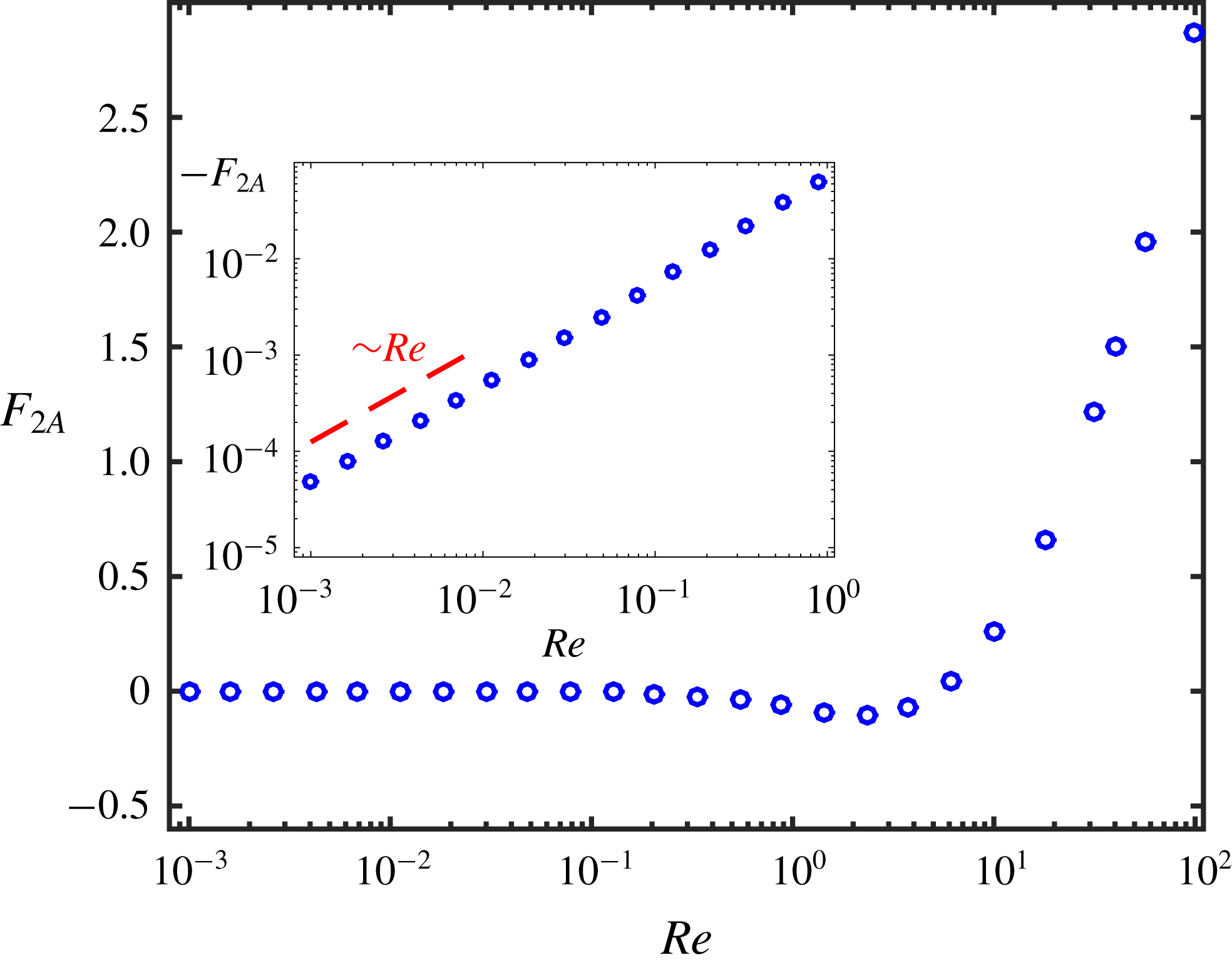
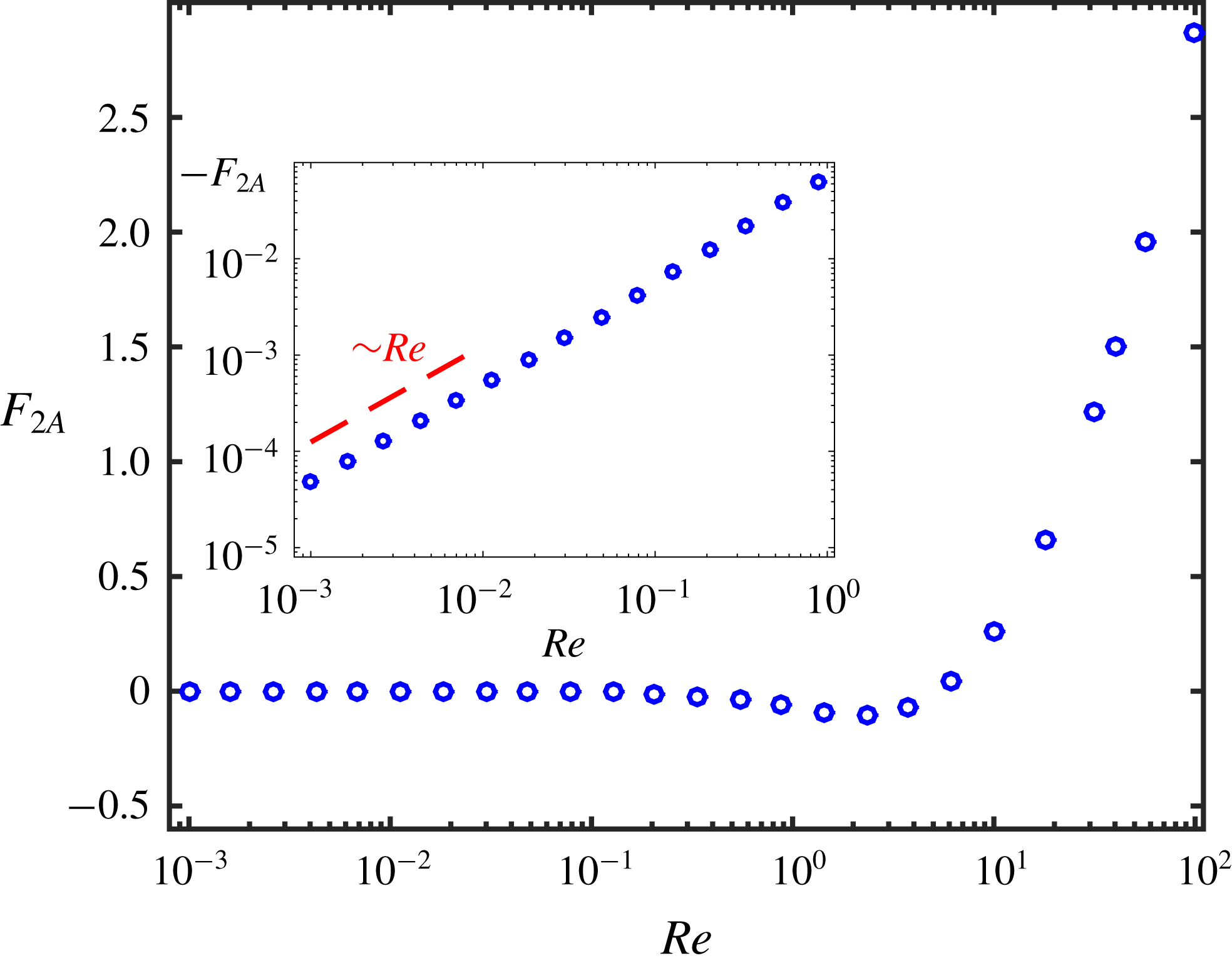
involves a coupling of the body shape and inertia. In figure 2,
 $F_{2A}$
is plotted versus
 $Re$
for the case of a prolate spheroid,
 $R(z)=\sqrt{1-z^{2}}$
, via numerical evaluation of the integral in (3.45).
Plot of
 $F_{2A}$
versus
 $Re$
for a prolate spheroid. The inset demonstrates that
 $F_{2A}\sim Re$
at small
 $Re$
.
The second inertial contribution to the drag is denoted
 $F_{2B}=-Re\int \tilde{\boldsymbol{v}}\boldsymbol{\cdot }(\boldsymbol{v}_{1}\boldsymbol{\cdot }\unicode[STIX]{x1D735}\boldsymbol{v}_{1})\,\text{d}V$
. The contribution to
 $F_{2B}$
from the inner region is
 $O[\unicode[STIX]{x1D716}\ln ^{2}(1/\unicode[STIX]{x1D716})]$
, which is negligibly small compared to the contribution from the outer region. Thus, in principle
 $F_{2B}$
can be evaluated in Fourier space; formally, we have
 $$\begin{eqnarray}F_{2B}=-Re\int \widehat{\boldsymbol{v}_{1}\boldsymbol{\cdot }\unicode[STIX]{x1D735}\boldsymbol{v}_{1}}(-\boldsymbol{k})\boldsymbol{\cdot }\hat{\tilde{\boldsymbol{v}}}(\boldsymbol{k})\,\text{d}\boldsymbol{k},\end{eqnarray}$$
where the Fourier transform of the material derivative is
 $$\begin{eqnarray}\widehat{\boldsymbol{v}_{1}\boldsymbol{\cdot }\unicode[STIX]{x1D735}\boldsymbol{v}_{1}}(\boldsymbol{k})=2\unicode[STIX]{x03C0}\text{i}\int \,\boldsymbol{k}\boldsymbol{\cdot }\hat{\boldsymbol{v}}_{1}(\boldsymbol{p})\hat{\boldsymbol{v}}_{1}(\boldsymbol{k}-\boldsymbol{p})\,\text{d}\boldsymbol{p}.\end{eqnarray}$$
Evaluating the integrals in (3.47) and (3.48) by hand requires a forbidding amount of algebra, due to the convolution of velocity fields in Fourier space. Therefore, instead, we evaluate
 $F_{2B}$
via a numerical quadrature in real space, using (3.12) and (3.32) to compute the velocity fields
 $\boldsymbol{v}_{1}$
and
 $\tilde{\boldsymbol{v}}$
, respectively. The integration is performed in cylindrical coordinates over the domain
 $0\leqslant r<\infty$
and
 $-\infty <z<\infty$
(note that the integrand is axisymmetric); it is permissible to take zero as the lower limit for
 $r$
since the inner region makes a negligibly small contribution to the integral. This also implies that
 $F_{2B}$
is independent of cross-sectional profile
 $R(z)$
. Practically, the upper limits of integration are truncated at finite values; careful attention is paid to ensure that the choice of these cutoffs do not affect the computed results. The velocity fields
 $\tilde{\boldsymbol{v}}$
and
 $\boldsymbol{v}_{1}$
both represent the flow due to a line distribution of Stokeslets at
 $Re=0$
and are, therefore, even functions of position,
 $\boldsymbol{x}$
. Hence, the integrand
 $\tilde{\boldsymbol{v}}\boldsymbol{\cdot }(\boldsymbol{v}_{1}\boldsymbol{\cdot }\unicode[STIX]{x1D735}\boldsymbol{v}_{1})$
should be an odd function of
 $\boldsymbol{x}$
; consequently, the integral itself vanishes at
 $Re=0$
. At small
 $Re$
we expect that the contribution to
 $\boldsymbol{v}_{1}$
that breaks the fore–aft symmetry of this velocity field is
 $O(Re)$
; hence,
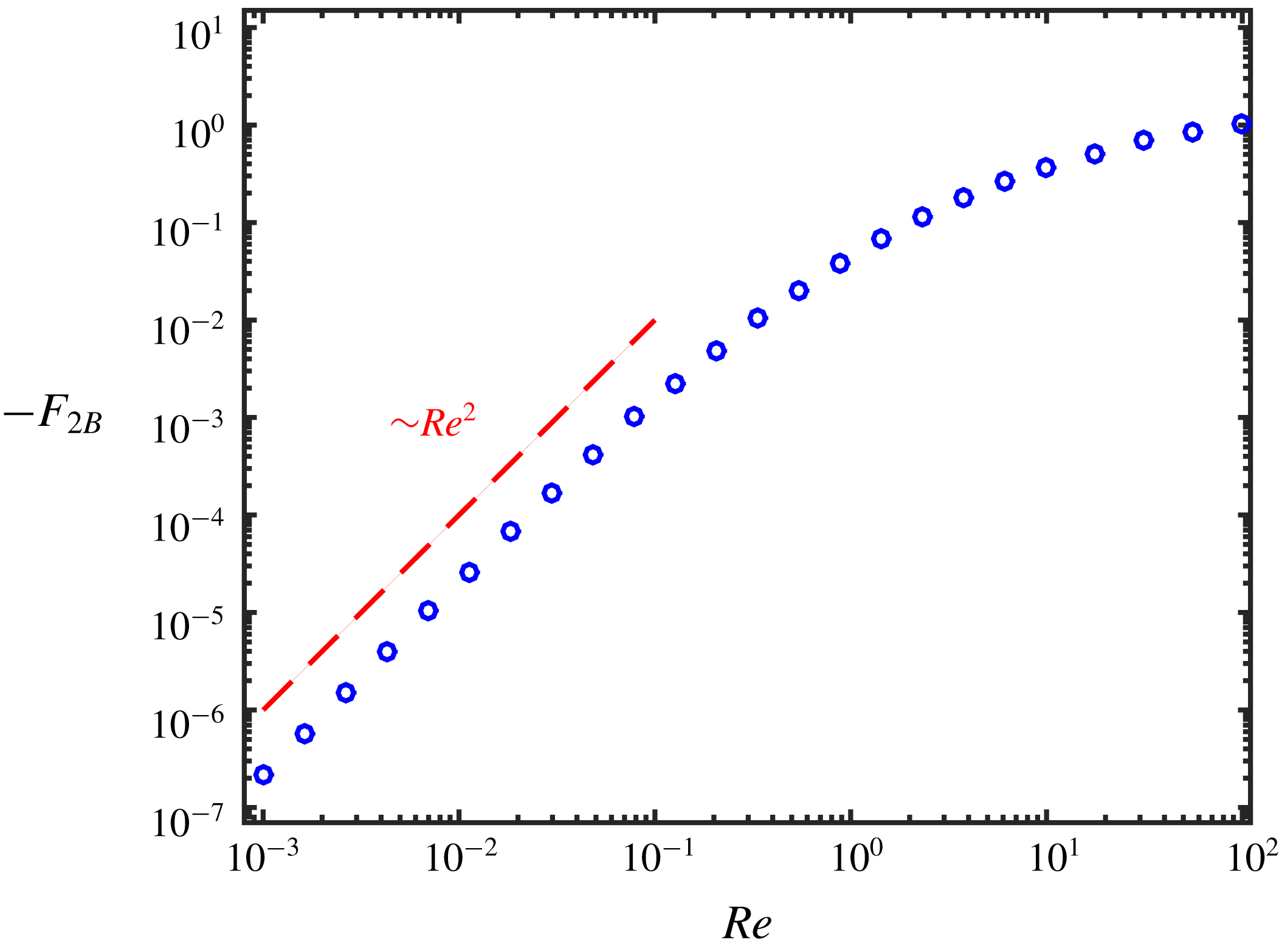
 $F_{2B}$
should scale as
 $Re^{2}$
for small
 $Re$
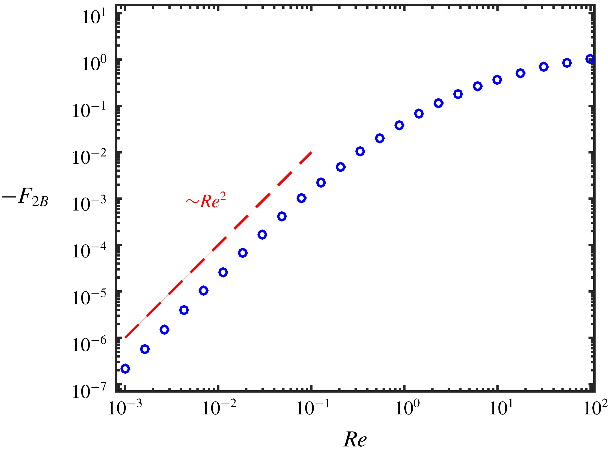
. Figure 3 plots the numerical evaluation of
 $F_{2B}$
versus
 $Re$
, where this scaling is evident.
Plot of
 $-F_{2B}$
versus
 $Re$
. The dashed line indicates that
 $F_{2B}\sim Re^{2}$
at small
 $Re$
.
We have determined the two inertial contributions to the drag at
 $O[1/\text{ln}^{3}(1/\unicode[STIX]{x1D716})]$
. There is an additional contribution, say
 $F_{2C}$
, arising from the creeping flow contribution to the force per unit length
 $f_{2}$
, say
 $f_{2}^{Re=0}$
, where (Tillett Reference Tillett1970)
 $$\begin{eqnarray}\frac{f_{2}^{Re=0}(z)}{2\unicode[STIX]{x03C0}}=\left(\ln \left[\frac{2(1-z^{2})^{1/2}}{R(z)}\right]-\frac{1}{2}\right)^{2}+\frac{1}{2}\int _{-1}^{1}\frac{\displaystyle \ln \left[\frac{(1-\unicode[STIX]{x1D709}^{2})^{1/2}}{R(\unicode[STIX]{x1D709})}\right]-\ln \left[\frac{(1-z^{2})^{1/2}}{R(z)}\right]}{|\unicode[STIX]{x1D709}-z|}\,\text{d}\unicode[STIX]{x1D709},\end{eqnarray}$$
and
 $F_{2C}=\int _{-1}^{1}f_{2}^{Re=0}(z)\,\text{d}z$
. Therefore, the total drag
 $F_{2}=F_{2A}+F_{2B}+F_{2C}$
.
4 Results and discussion
The inertial enhancement of the drag is characterized by the ratio
 $F(Re)/F(0)$
, which, from the analysis above, is
 $$\begin{eqnarray}\displaystyle \frac{F(Re)}{F(0)} & = & \displaystyle 1+\frac{F_{1}(Re)-F_{1}(0)}{4\unicode[STIX]{x03C0}\ln (1/\unicode[STIX]{x1D716})}\nonumber\\ \displaystyle & & \displaystyle +\,\frac{1}{4\unicode[STIX]{x03C0}\ln ^{2}(1/\unicode[STIX]{x1D716})}\left(F_{2}(Re)-F_{2}(0)+[F_{1}(0)-F_{1}(Re)]\frac{F_{1}(0)}{4\unicode[STIX]{x03C0}}\right)\nonumber\\ \displaystyle & & \displaystyle +\,O\left(\frac{1}{\ln ^{3}(1/\unicode[STIX]{x1D716})}\right).\end{eqnarray}$$
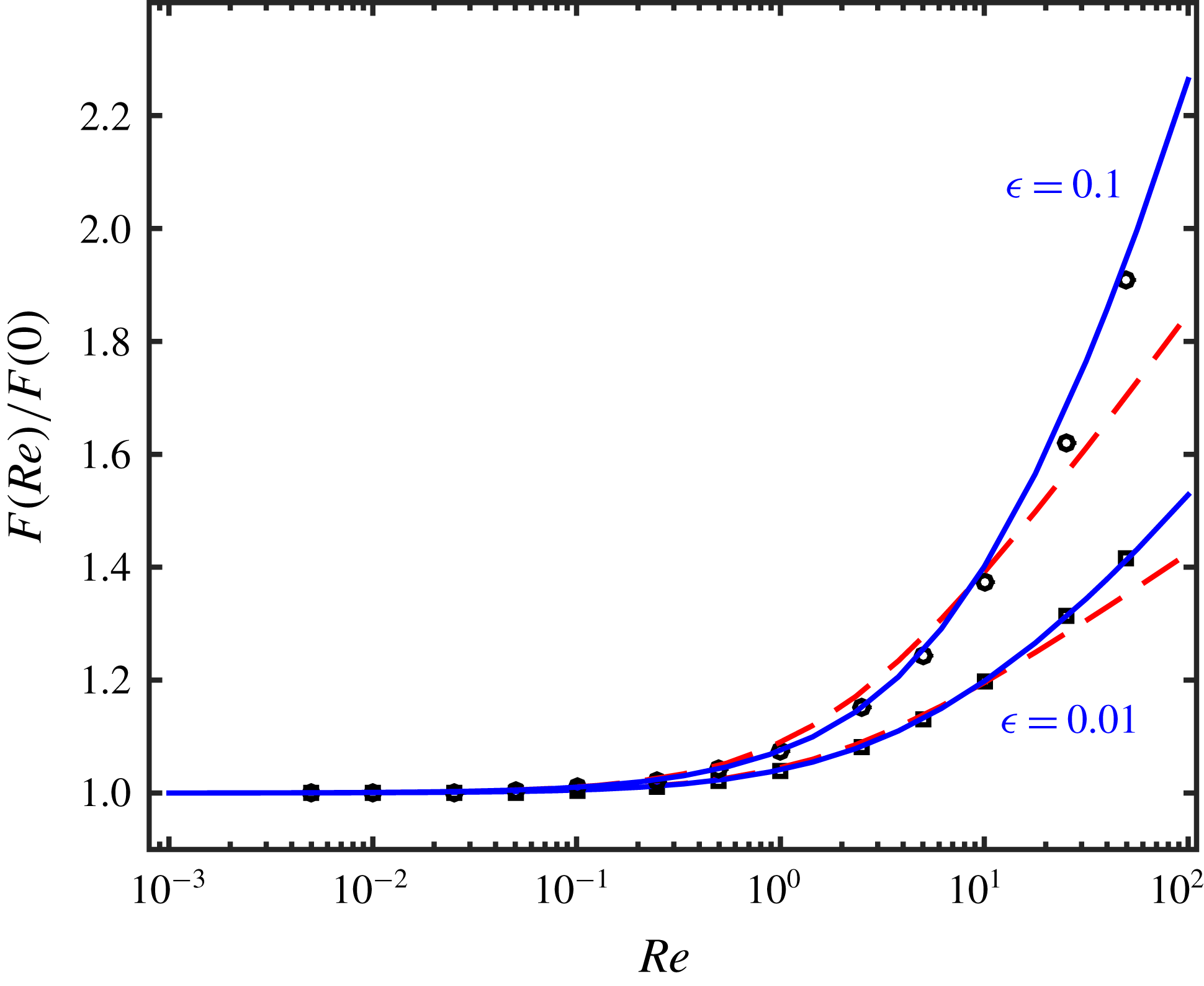
Let us first consider a prolate spheroid. The values of
 $F(Re)/F(0)$
from (4.1) in this case are plotted in figure 4 for
 $\unicode[STIX]{x1D716}=0.1$
and
 $\unicode[STIX]{x1D716}=0.01$
. The figure also displays the values of
 $F(Re)/F(0)$
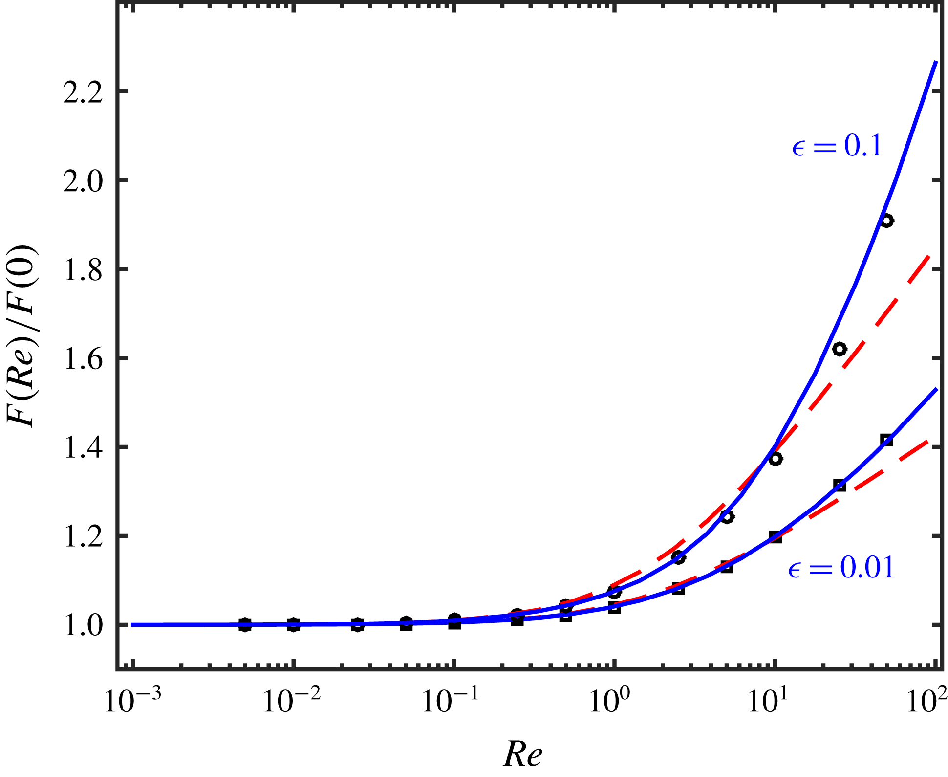
from a numerical solution of the Navier–Stokes equations; details of the numerical method are in appendix C. The agreement between the asymptotic and numerical evaluations is surprisingly good, given the logarithmic in
 $\unicode[STIX]{x1D716}$
error in the expansion (4.1). The figure also displays
 $F(Re)/F(0)$
retaining terms through
 $O(1/\text{ln}(1/\unicode[STIX]{x1D716}))$
, as determined by Khayat & Cox (Reference Khayat and Cox1989). As expected, the agreement between the asymptotics and numerics is improved when the former includes terms through
 $O(1/\text{ln}^{2}(1/\unicode[STIX]{x1D716}))$
, as determined in the present work. From the data at
 $\unicode[STIX]{x1D716}=0.1$
, it is evident that the asymptotic and numeric results begin to deviate at around
 $Re=20$
, which is consistent with the loss of uniformity in the expansion (4.1) at
 $Re=O(1/\unicode[STIX]{x1D716})$
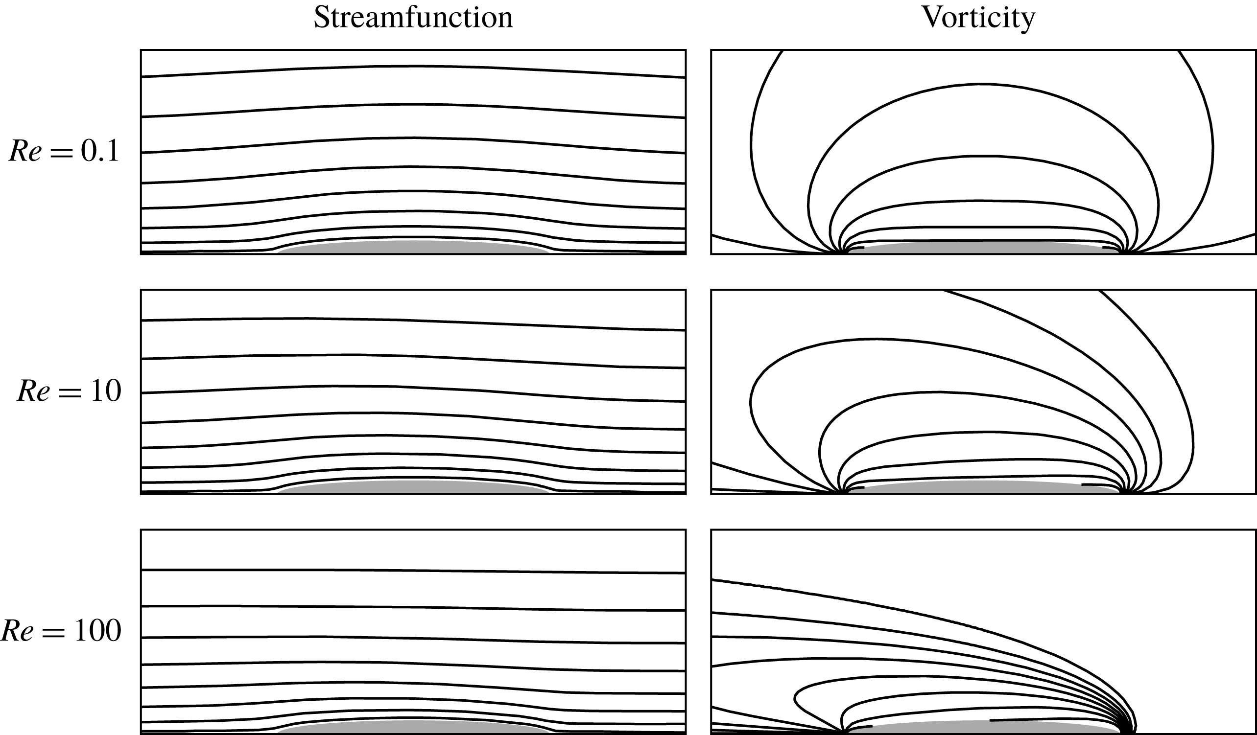
. We emphasize that inertia forces result in significant fore–aft flow asymmetry at
 $Re=O(1/\unicode[STIX]{x1D716})$
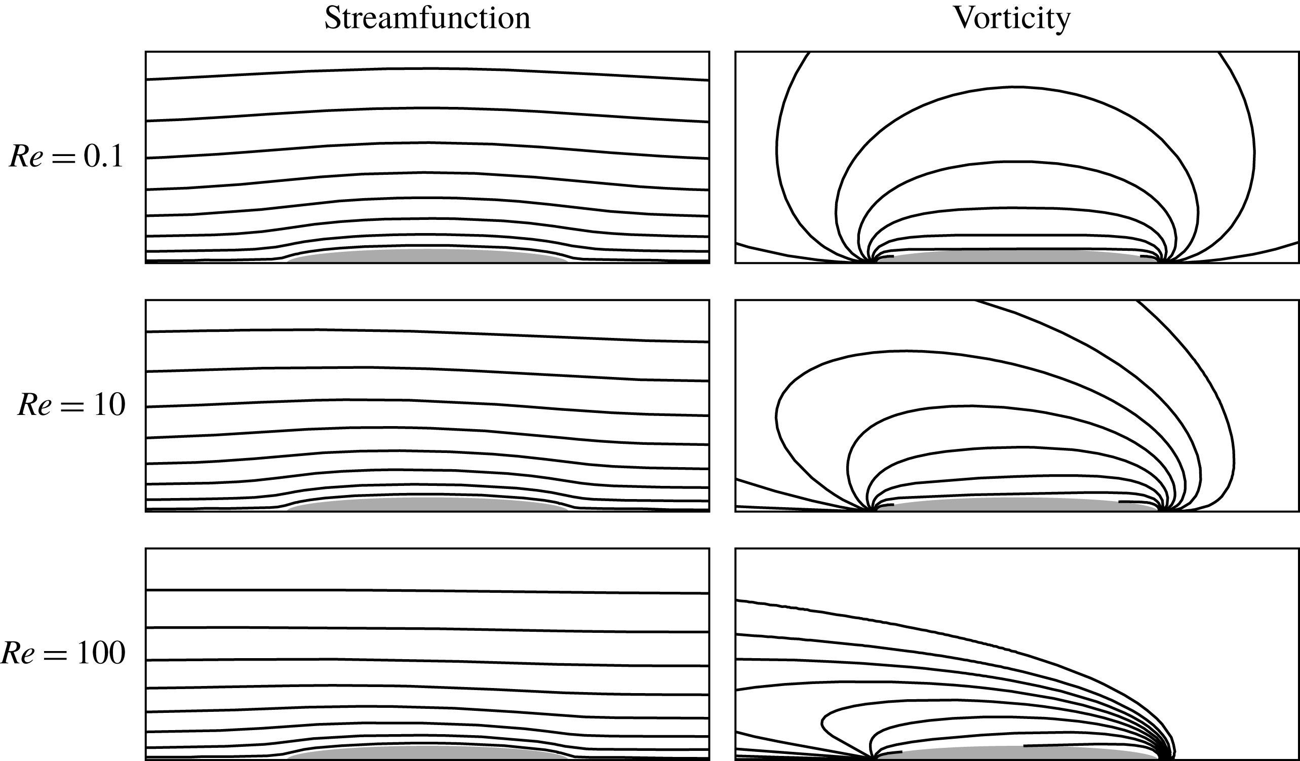
. For example, figure 5 displays the numerically computed streamlines and vorticity contours at
 $\unicode[STIX]{x1D716}=0.1$
for
 $Re=0.1,10$
and
 $100$
. Viewed in the co-moving frame, the streamlines belie the fore–aft asymmetric nature of the flow at
 $Re=10$
and
 $100$
, which is unmasked by considering the vorticity profile. Specifically, the effect of inertia in sweeping vorticity past the spheroid is evident.
Plot of
 $F(Re)/F(0)$
versus
 $Re$
for a prolate spheroid. The symbols are from numerical solution of the Navier–Stokes equations at
 $\unicode[STIX]{x1D716}=0.1$
(circles) and
 $\unicode[STIX]{x1D716}=0.01$
(squares). The dashed lines represent the asymptotic expression for
 $F(Re)/F(0)$
through
 $O[1/\text{ln}(1/\unicode[STIX]{x1D716})]$
, and the solid lines are
 $F(Re)/F(0)$
through
 $O[1/\text{ln}^{2}(1/\unicode[STIX]{x1D716})]$
.
Numerically computed streamlines and vorticity contours around a prolate spheroid with
 $\unicode[STIX]{x1D716}=0.1$
.
The favourable comparison of the asymptotic and numerical results warrants further comment. It can happen that a slender-body approximation yields results in good agreement with numerics at moderately small values of the slenderness parameter
 $\unicode[STIX]{x1D716}$
, in spite of the inherent logarithmic error of the asymptotic expansion. This may occur because only the first couple of coefficients of the expansion are non-zero, with the implication that the error is then algebraically small in
 $\unicode[STIX]{x1D716}$
. A recent example thereof is provided by Schnitzer & Yariv (Reference Schnitzer and Yariv2015), who used slender-body theory to predict the rectilinear velocity of a spheroidal particle undergoing self-diffusiophoresis; their results compare remarkably well to a numerical computation by Popescu et al. (Reference Popescu, Dietrich, Tasinkevych and Ralston2011) at
 $\unicode[STIX]{x1D716}=0.1$
. A second possibility is that all the terms in the logarithmic expansion can be calculated. Batchelor (Reference Batchelor1970) showed that this is possible for the force, torque, and stresslet on a particle (in Stokes flow) that is ‘longitudinally elliptic’ and whose cross-section shape and orientation (but not size) is independent of the coordinate along the centreline of the body (e.g. an ellipsoid). In this case, the error in the slender-body approximation is again algebraic. In the present work, there is no reason to expect that the next,
 $O(1/\text{ln}^{4}(1/\unicode[STIX]{x1D716}))$
, term of the drag expansion is zero for a prolate spheroid, let alone a particle with more complex shape, due to inertia breaking the fore–aft symmetry of the flow in the outer region. This makes the agreement between the asymptotics and numerics in figure 4 all the more surprising. Continuing the expansion to
 $O(1/\text{ln}^{4}(1/\unicode[STIX]{x1D716}))$
is a very difficult task, since an expression for
 $f_{2}$
is unavailable. Indeed, this escalation in technical difficulty is a common feature of logarithmic expansions for which the outer problem is governed by a nonlinear or non-constant coefficient equation. The prototypical example thereof is uniform flow past a cylinder; here, only the first few terms in the outer flow can be calculated analytically. An interesting alternative approach to this problem, which can in principle incorporate all logarithmic orders, is the hybrid asymptotic–numerical method of Kropinksi, Ward & Keller (Reference Khayat, Ward and Keller1995) and Hormozi & Ward (Reference Hormozi and Ward2017). Here, the outer problem, i.e. the Navier–Stokes equations, is not expanded in powers of
 $1/\text{ln}(1/\unicode[STIX]{x1D716})$
; instead, it is solved numerically subject to a specified singular forcing as
 $r\rightarrow 0$
(i.e. as the inner region is approach). Matching the numerical outer solution to the inner solution (which satisfies the Stokes equations) yields a transcendental equation for the coefficient of the singular forcing term. From solution of this equation, the drag on a cylinder can computed though all logarithmic orders. It would be interesting, in future work, to see if a similar hybrid approach could be applied to the present problem.
At the present level of approximation, the sole coupling of inertia to the body profile is contained within the
 $F_{2A}$
contribution to
 $F_{2}$
. Rearranging (3.45) gives
 $$\begin{eqnarray}\frac{F_{2A}}{4\unicode[STIX]{x03C0}}=\frac{1}{8}\int _{-1}^{1}\left(G-\frac{1}{Re}\frac{\text{d}G}{\text{d}s}-1\right){\mathcal{G}}(-s)-2\left[\ln \left(\frac{2(1-s^{2})^{1/2}}{R(s)}\right)-\frac{1}{2}\right][{\mathcal{G}}(s)+{\mathcal{G}}(-s)]\,\text{d}s.\end{eqnarray}$$
Consider two profiles
 $R_{1}$
and
 $R_{2}$
that are mirror symmetric,
 $R_{2}(-s)=R_{1}(s)$
. Evidently, from (4.2) the value of
 $F_{2A}$
is identical for these two cases. Therefore, the drag on a slender particle is insensitive to its direction of travel through
 $O[1/\text{ln}^{3}(1/\unicode[STIX]{x1D716})]$
. This is a surprising result given that the Reynolds number is not restricted to be small; recall, we require only that
 $Re\ll O(1/\unicode[STIX]{x1D716})$
for uniformity of the asymptotic expansion. The reason is that the value of
 $F_{2A}$
is the same as that would occur from a slender-body analysis of the Oseen equations; the drag on a fore–aft symmetric particle predicted from the Oseen equations is insensitive to the travel direction at arbitrary
 $Re$
(Olmstead & Gautesen Reference Olmstead and Gautesen1968). Recall, the difference between the drag on a slender body at
 $O[1/\text{ln}^{3}(1/\unicode[STIX]{x1D716})]$
predicted from the Navier–Stokes and Oseen equations arises from
 $F_{2B}$
, which is independent of the body profile. A corollary is that our slender-body analysis predicts that a ‘perfect projectile’, i.e. a body of fixed volume that experiences the least drag in steady translation, must be fore–aft symmetric through
 $O[1/\text{ln}^{3}(1/\unicode[STIX]{x1D716})]$
. This finding is consistent with Roper, Squires & Brenner (Reference Roper, Squires and Brenner2008) who demonstrated, via numerical solution of the Navier–Stokes equations, that a perfect projectile remains approximately fore–aft symmetric up to moderate
 $Re$
, even though the flow around it is markedly asymmetric. Interestingly, their calculations show that the slenderness of a perfect projectile increases with increasing
 $Re$
: from a rough analysis of their figure 1(a), a perfect projectile has
 $\unicode[STIX]{x1D716}\approx 0.5$
at
 $Re=0.1$
and
 $\unicode[STIX]{x1D716}\approx 0.2$
at
 $Re=100$
. However, Roper et al. (Reference Roper, Squires and Brenner2008) also showed, via asymptotic analysis at
 $Re\ll 1$
, that there is weak
 $O(Re^{3})$
fore–aft asymmetry in the projectile shape for arbitrarily small Reynolds numbers. We believe that an equivalent weak asymmetry would occur in the next,
 $O[1/\text{ln}^{4}(1/\unicode[STIX]{x1D716})]$
, term in the slender-body expansion for
 $F$
, which must therefore be sensitive to the direction of travel. Here, the weakness of the asymmetry refers to the smallness of
 $\unicode[STIX]{x1D716}$
, rather than
 $Re$
.
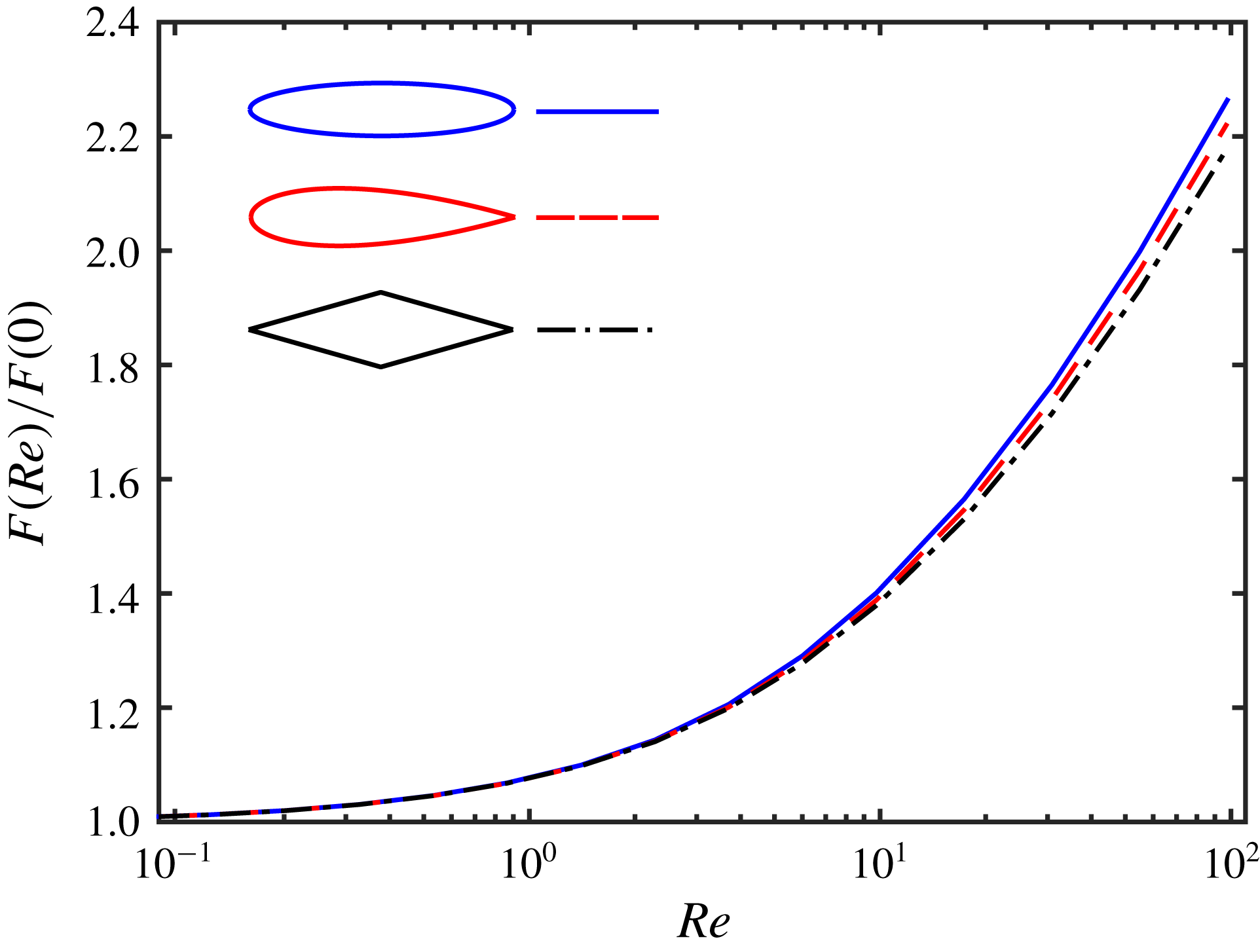
Plot of
 $F(Re)/F(0)$
versus
 $Re$
at
 $\unicode[STIX]{x1D716}=0.1$
for three particle shapes.
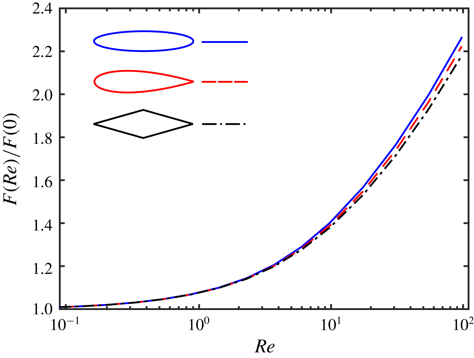
In figure 6 the ratio
 $F(Re)/F(0)$
from (4.1) is plotted for three different shapes of equal volume: (i) a prolate spheroid; (ii)
 $R(z)=\sqrt{(1-z)(1-z^{2})}$
, which resembles an airfoil; and (iii) a double cone,
 $R(z)=\sqrt{2}[1-z\,\text{sgn}(z)]$
. Shape (ii) is fore–aft asymmetric,
 $R(z)\neq R(-z)$
. However, from the discussion in the above paragraph, the direction of travel for this shape does not affect the drag. For a fixed value of
 $Re$
, the ratio
 $F(Re)/F(0)$
is largest for case (i) and smallest for case (iii), which indicates that the inertial drag is reduced by the pointed ends of a body. However, the effect is not large, which is symptomatic of the weak (logarithmic) dependence of the drag on the shape of a slender body at the moderate
 $Re$
. Nonetheless, it is worthwhile to mention that our analysis can be extended to a particle possessing a transverse cross-section of arbitrary shape with a modicum of effort. Specifically, when the uniform stream is aligned with the centreline of the body, the velocity field in the inner region for a particle with a non-circular cross-section is predominantly axial and may be written as (Batchelor Reference Batchelor1970)
 $$\begin{eqnarray}w=\frac{f(z;\unicode[STIX]{x1D716})}{2\unicode[STIX]{x03C0}}\ln \frac{\unicode[STIX]{x1D70C}}{R^{\ast }(z)}+O\left(\frac{1}{\unicode[STIX]{x1D70C}}\right),\end{eqnarray}$$
for
 $\unicode[STIX]{x1D70C}\gg 1$
. Here,
 $R^{\ast }(z)$
is the radius of the circular cross-section that is equivalent to the actual (non-circular) cross-section, in the sense that the flow at
 $\unicode[STIX]{x1D70C}\gg 1$
is the same in both cases, given the same axial force distribution. As noted by Batchelor (Reference Batchelor1970), since the inner region is dominated by vorticity diffusion (provided
 $\unicode[STIX]{x1D716}^{2}Re\ll 1$
), the flow there tends to an axisymmetric form before the outer region is reached. Hence, the matching process between inner and outer regions is essentially unaltered; one simply replaces
 $R(z)$
by
 $R^{\ast }(z)$
to generalize the preceding results for the drag on an axisymmetric particle to a particle with an arbitrary cross-section. The form of
 $R^{\ast }$
for a particular cross-section shape can be found by conformal mapping: several interesting cases are given by Batchelor (Reference Batchelor1970) and Hinch (Reference Hinch1991). For an ellipse
 $R^{\ast }=(b+c)/2$
, where
 $b$
and
 $c$
are the dimensionless semi-diameters, normalized by the width scale
 $a$
. Here,
 $R^{\ast }$
ranges between unity (for a circle,
 $b=c=1$
) to one half (for a flat plate,
 $b=1$
and
 $c=0$
).
It would be of interest to generalize our analysis to a particle whose centreline is oblique to the uniform stream; one expects that the inertial torque and lift force, in addition to the drag, are dependent on particle shape at
 $O[1/\text{ln}^{3}(1/\unicode[STIX]{x1D716})]$
. This generalization is conceptually straightforward: the lift, drag and torque at this order can be calculated via the generalized reciprocal theorem. Of course, now the velocity field is not axisymmetric, which adds to the technical complexity of the calculation. However, some general remarks can be made without detailed calculation. The dependence of the
 $O[1/\text{ln}^{3}(1/\unicode[STIX]{x1D716})]$
drag on the body shape occurs solely from the contribution
 $F_{2A}$
, which is exactly the same as one would obtain from a slender-body analysis of the Oseen equations. (That is, the difference in drag predicted from a slender-body analysis of the Navier–Stokes equations and Oseen equations arises from
 $F_{2B}$
, which is independent of body shape.) For the Oseen equations, Olmstead & Gautesen (Reference Olmstead and Gautesen1968) proved that the drag on a particle of arbitrary shape is left unchanged in magnitude upon a reversal in direction of the uniform stream. Therefore, the insensitivity of the
 $O[1/\text{ln}^{3}(1/\unicode[STIX]{x1D716})]$
drag we predict for the Navier–Stokes equations must persist for all orientations of the particle with respect to the stream. However, Olmstead & Gautesen (Reference Olmstead and Gautesen1968) also note that the magnitude of the lift force computed from the Oseen equations is not necessarily invariant to the flow direction. Hence, there is no reason to expect that the
 $O[1/\text{ln}^{3}(1/\unicode[STIX]{x1D716})]$
lift is insensitive to fore–aft asymmetry of the body shape.
Acknowledgements
A.S.K. acknowledges the support from a Carnegie Institute of Technology Dean’s Early Career Fellowship.
Appendix A. Leading-order term of
 $v_{2}$
as
$r\rightarrow 0$


Herein a leading-order approximation of the
 $O[1/\text{ln}^{2}(1/\unicode[STIX]{x1D716})]$
velocity field
 $\boldsymbol{v}_{2}$
as
 $r\rightarrow 0$
is derived, following the method of Schnitzer (Reference Schnitzer2015). The axial component of the momentum balance (3.22) is
 $$\begin{eqnarray}Re\frac{\unicode[STIX]{x2202}w_{2}}{\unicode[STIX]{x2202}z}-\left[\frac{1}{r}\frac{\unicode[STIX]{x2202}}{\unicode[STIX]{x2202}r}\left(r\frac{\unicode[STIX]{x2202}w_{2}}{\unicode[STIX]{x2202}r}\right)+\frac{\unicode[STIX]{x2202}^{2}w_{2}}{\unicode[STIX]{x2202}z^{2}}\right]+\frac{\unicode[STIX]{x2202}p_{2}}{\unicode[STIX]{x2202}z}=-Re\,\boldsymbol{e}_{z}\boldsymbol{\cdot }(\boldsymbol{v}_{1}\boldsymbol{\cdot }\unicode[STIX]{x1D735}\boldsymbol{v}_{1}),\end{eqnarray}$$
where
 $w_{2}$
is the axial component of
 $\boldsymbol{v}_{2}$
. From (3.12) with
 $h_{1}(z)=2\unicode[STIX]{x03C0}$
we find
 $$\begin{eqnarray}\boldsymbol{v}_{1}\sim \left(2\ln r-\frac{K}{2}\right)\boldsymbol{e}_{z}-\frac{1}{2Re}\unicode[STIX]{x1D735}G+o(1),\end{eqnarray}$$
as
 $r\rightarrow 0$
, where
 $K(z)=2\ln [2(1-z^{2})^{1/2}]-G(z)$
. Thus, as
 $r\rightarrow 0$
the axial velocity
 $$\begin{eqnarray}w_{1}\sim 2\ln r-\frac{K}{2}-\frac{1}{2Re}\frac{\unicode[STIX]{x2202}G}{\unicode[STIX]{x2202}z}+o(1).\end{eqnarray}$$
Application of the continuity equation and (A 3) yields the limiting form of the radial component of
 $\boldsymbol{v}_{1}$
, say
 $u_{1}$
, as
 $$\begin{eqnarray}u_{1}\sim \frac{1}{4}\left(\frac{\text{d}K}{\text{d}z}+\frac{1}{Re}\frac{\text{d}^{2}G}{\text{d}z^{2}}\right)r+o(r).\end{eqnarray}$$
Therefore, as
 $r\rightarrow 0$
the body force
 $$\begin{eqnarray}-Re\boldsymbol{v}_{1}\boldsymbol{\cdot }\unicode[STIX]{x1D735}\boldsymbol{v}_{1}\sim \frac{Re}{2}\left(\frac{\text{d}K}{\text{d}z}+\frac{1}{Re}\frac{\text{d}^{2}G}{\text{d}z^{2}}\right)\ln r\boldsymbol{e}_{z}-\frac{Re}{4}\left(\frac{\text{d}^{2}K}{\text{d}z^{2}}+\frac{1}{Re}\frac{\text{d}^{3}G}{\text{d}z^{3}}\right)r\ln r\boldsymbol{e}_{r}+o(r\ln r).\end{eqnarray}$$
The pressure satisfies the Poisson equation
 $\unicode[STIX]{x1D6FB}^{2}p_{2}=-Re\unicode[STIX]{x1D735}\boldsymbol{\cdot }(\boldsymbol{v}_{1}\boldsymbol{\cdot }\unicode[STIX]{x1D735}\boldsymbol{v}_{1})$
, and using (A 5) it is readily shown that the forcing
 $\unicode[STIX]{x1D735}\boldsymbol{\cdot }(\boldsymbol{v}_{1}\boldsymbol{\cdot }\unicode[STIX]{x1D735}\boldsymbol{v}_{1})$
does not contain a term proportional to
 $\ln r$
. Therefore,
 $p_{2}$
cannot contain a term proportional to
 $\ln r$
; otherwise, the term
 $\unicode[STIX]{x2202}^{2}p_{2}/\unicode[STIX]{x2202}z^{2}$
in the Poisson equation would be unbalanced. Therefore, in (A 1) the leading-order (logarithmic) forcing originates solely from the body force. To obtain the leading-order behaviour of the particular solution to (A 1) we pose the ansatz
 $w_{2P}\sim A(z)\ln r$
, which yields the following equation for
 $A(z)$
,
 $$\begin{eqnarray}\frac{\text{d}^{2}A}{\text{d}z^{2}}-Re\frac{\text{d}A}{\text{d}z}=-\frac{Re}{2}\left(\frac{\text{d}K}{\text{d}z}+\frac{1}{Re}\frac{\text{d}^{2}G}{\text{d}z^{2}}\right).\end{eqnarray}$$
The solution to (A 6) is
 $$\begin{eqnarray}\displaystyle A(z) & = & \displaystyle \frac{\unicode[STIX]{x1D6FE}}{2}+\frac{1}{2}\ln Re(1+z)-\frac{1}{2}E_{1}[Re(1-z)]+\frac{1}{2}\text{e}^{Re(z-1)}E_{1}[Re(z-1)]\nonumber\\ \displaystyle & & \displaystyle +\,\frac{1}{2}\text{e}^{Re(1+z)}E_{1}[Re(1+z)].\end{eqnarray}$$
In deriving (A 7), we have chosen the constants of integration belonging to the complementary solution to (A 6) such that (A 7) vanishes at
 $Re=0$
, since a non-zero particular solution
 $w_{2P}$
occurs solely due to inertia. In fact, at small
 $Re$
 $$\begin{eqnarray}A(z)\sim {\textstyle \frac{1}{2}}[(3-2\unicode[STIX]{x1D6FE})z-1+(1+z)\ln (1+z)+(1-z)\ln (1-z)]Re-zRe\ln Re+O(Re^{2}).\end{eqnarray}$$
The radial component of the particular solution,
 $u_{2P}$
, may be found from the continuity equation if desired. The complementary solution
 $\boldsymbol{v}_{2H}$
is of the form (3.12), with a new source density,
 $h_{2}(z)$
say. Per (3.14), as
 $r\rightarrow 0$
the axial component
 $w_{2H}\sim (h_{2}/2\unicode[STIX]{x03C0})\ln r+O(1)$
. Thus, matching
 $\boldsymbol{v}_{2}$
as
 $r\rightarrow 0$
with the inner solution (cf. (3.15)) yields
 $h(z)=f_{1}(z)-2\unicode[STIX]{x03C0}A(z)$
. We have thus determined the leading-order approximation to the outer velocity field at
 $O[1/\text{ln}^{2}(1/\unicode[STIX]{x1D716})]$
as
 $r\rightarrow 0$
. To determine the force per unit length on the particle at
 $O[1/\text{ln}^{3}(1/\unicode[STIX]{x1D716})]$
, namely
 $f_{2}(z)$
, would require determining the
 $O(1)$
correction to
 $\boldsymbol{v}_{2}$
as
 $r\rightarrow 0$
. Fortunately, use of the generalized reciprocal theorem enables one to determine the drag at
 $O[1/\text{ln}^{3}(1/\unicode[STIX]{x1D716})]$
without computing
 $f_{2}$
.
Appendix B. The Fourier integral in (3.42)
Below we outline the evaluation of the Fourier integral in (3.42). Essentially the same integral was encountered by Subramanian & Koch (Reference Subramanian and Koch2005) in calculating the inertial torque on a sedimenting slender body. However, those authors did not give the result for the integral itself; rather, they presented the final expression for the inertial torque. Given the importance of this integral to the present work it is appropriate for us to give an explanation of its evaluation. The integral is split as
 $I_{1}-I_{2}$
, where
 $$\begin{eqnarray}\left.\begin{array}{@{}c@{}}\displaystyle I_{1}=\int \frac{(\boldsymbol{e}_{z}\boldsymbol{\cdot }\boldsymbol{k})\text{e}^{2\unicode[STIX]{x03C0}\text{i}(s-s^{\prime })\boldsymbol{e}_{z}\boldsymbol{\cdot }\boldsymbol{k}}}{(2\unicode[STIX]{x03C0}k^{2})[(2\unicode[STIX]{x03C0}k)^{2}-2\unicode[STIX]{x03C0}\text{i}Re\boldsymbol{e}_{z}\boldsymbol{\cdot }\boldsymbol{k}]}\,\text{d}\boldsymbol{k},\quad \text{and}\\ \displaystyle I_{2}=\int \frac{(\boldsymbol{e}_{z}\boldsymbol{\cdot }\boldsymbol{k})^{3}\text{e}^{2\unicode[STIX]{x03C0}\text{i}(s-s^{\prime })\boldsymbol{e}_{z}\boldsymbol{\cdot }\boldsymbol{k}}}{(2\unicode[STIX]{x03C0}k^{4})[(2\unicode[STIX]{x03C0}k)^{2}-2\unicode[STIX]{x03C0}\text{i}Re\boldsymbol{e}_{z}\boldsymbol{\cdot }\boldsymbol{k}]}\,\text{d}\boldsymbol{k}.\end{array}\right\}\end{eqnarray}$$
We adopt a Fourier-space coordinate system
 $\boldsymbol{k}=k_{1}\boldsymbol{e}_{z}+\boldsymbol{k}_{t}$
, where
 $\boldsymbol{k}_{t}=(k_{2},k_{3})$
is a vector in the plane transverse to
 $\boldsymbol{e}_{z}$
. Therefore,
 $$\begin{eqnarray}I_{1}=\frac{1}{(2\unicode[STIX]{x03C0})^{4}}\int _{-\infty }^{\infty }\text{d}q_{3}\int _{-\infty }^{\infty }\text{d}q_{2}\int _{-\infty }^{\infty }\frac{q_{1}\text{e}^{\text{i}(s-s^{\prime })q_{1}}}{q^{2}(q^{2}-\text{i}Req_{1})}\,\text{d}q_{1},\end{eqnarray}$$
where
 $\boldsymbol{q}=2\unicode[STIX]{x03C0}\boldsymbol{k}$
. The integral over
 $q_{1}$
is performed using the residue theorem. For
 $s-s^{\prime }>0$
the integration contour is closed by a semicircular arc in the upper half-plane. By Jordan’s lemma, the contribution to the integral from the arc vanishes as its radius goes to infinity. The integrand has two simple poles in the upper half-plane, which are located at
 $$\begin{eqnarray}q_{1,a}=\text{i}q_{t},\quad \text{and}\quad q_{1,b}=\frac{\text{i}}{2}[Re+(Re^{2}+4q_{t}^{2})^{1/2}],\end{eqnarray}$$
where
 $q_{t}=(q_{2}^{2}+q_{3}^{2})^{1/2}$
. Therefore, the integral over
 $q_{1}$
equals
 $2\unicode[STIX]{x03C0}\text{i}[\text{Res}(q_{1a})+\text{Res}(q_{1b})]$
, where the residues are given by
 $$\begin{eqnarray}\displaystyle & \displaystyle \text{Res}(q_{1a})=\frac{\text{e}^{-(s-s^{\prime })q_{t}}}{2Req_{t}}, & \displaystyle\end{eqnarray}$$
 $$\begin{eqnarray}\displaystyle & \displaystyle \text{Res}(q_{1b})=-\frac{\text{e}^{-(1/2)(s-s^{\prime })[Re+(Re^{2}+4q_{t}^{2})^{1/2}]}}{Re(Re^{2}+4q_{t}^{2})^{1/2}}. & \displaystyle\end{eqnarray}$$
The integrations over
 $q_{2}$
and
 $q_{3}$
are carried out in plane polar coordinates,
 $q_{2}=q_{t}\cos \unicode[STIX]{x1D719}$
and
 $q_{3}=q_{t}\sin \unicode[STIX]{x1D719}$
. The integration over
 $\unicode[STIX]{x1D719}$
simply yields
 $2\unicode[STIX]{x03C0}$
(due to the axisymmetry of the velocity field), leaving
 $$\begin{eqnarray}I_{1}=\frac{\text{i}}{4\unicode[STIX]{x03C0}^{2}}\int _{0}^{\infty }[\text{Res}(q_{1a})+\text{Res}(q_{1b})]q_{t}\,\text{d}q_{t}=\frac{\text{i}}{8\unicode[STIX]{x03C0}^{2}Re}\left(\frac{1-\text{e}^{-(s-s^{\prime })Re}}{s-s^{\prime }}\right),\end{eqnarray}$$
which is valid for
 $s-s^{\prime }>0$
. For
 $s-s^{\prime }<0$
the contour is closed by a semicircular arc in the lower half-plane, in which there are two simple poles, and it can be shown that that
 $I_{1}=0$
in this case. The integral
 $I_{2}$
is evaluated in a similar manner. Here, for the integration over
 $q_{1}$
when
 $s-s^{\prime }>0$
, the integrand has the same two poles in the upper half-plane, but now
 $q_{1a}=\text{i}q_{t}$
is a double pole, whereas
 $q_{1b}$
remains a simple pole. Therefore, the integral over
 $q_{1}$
equals
 $2\unicode[STIX]{x03C0}\text{i}[\text{Res}(q_{1a})+\text{Res}(q_{1b})]$
, in which
 $$\begin{eqnarray}\displaystyle & \displaystyle \text{Res}(q_{1a})=\frac{\text{e}^{-(s-s^{\prime })q_{t}}(Re+2q_{t}+(s^{\prime }-s)Req_{t})}{4Re^{2}q_{t}}, & \displaystyle\end{eqnarray}$$
 $$\begin{eqnarray}\displaystyle & \displaystyle \text{Res}(q_{1b})=-\frac{\text{e}^{-(1/2)(s-s^{\prime })[Re+(Re^{2}+4q_{t}^{2})^{1/2}]}(Re+(Re^{2}+4q_{t}^{2})^{1/2})}{2Re^{2}(Re^{2}+4q_{t}^{2})^{1/2}}, & \displaystyle\end{eqnarray}$$
 $$\begin{eqnarray}I_{2}=\frac{\text{i}}{4\unicode[STIX]{x03C0}^{2}}\int _{0}^{\infty }[\text{Res}(q_{1,a})+\text{Res}(q_{1,b})]q_{r}\,\text{d}q_{r}=\frac{\text{i}}{8\unicode[STIX]{x03C0}^{2}Re}\left[\frac{\text{e}^{-(s-s^{\prime })Re}-1}{(s-s^{\prime })^{2}Re}+\frac{\text{e}^{-(s-s^{\prime })Re}}{s-s^{\prime }}\right],\end{eqnarray}$$
which is valid for
 $s-s^{\prime }>0$
. It can be shown that
 $I_{2}=0$
for
 $s-s^{\prime }<0$
. Combination of (B 5) and (B 7) yields (3.43), where
 ${\mathcal{H}}(t,s)$
is defined in (3.44).
Appendix C. Numerical solution method
The flow past a prolate spheroid was numerically solved using a spectral element method for the aspect ratios
 $\unicode[STIX]{x1D700}=0.1$
and
 $\unicode[STIX]{x1D700}=0.01$
. A custom code was implemented in Python using the numpy and scipy numerical libraries. The same code was used by Chisholm et al. (Reference Chisholm, Lauga, Legendre and Khair2016) to compute the flow past a sphere propelled by a surface slip velocity, and more details (including code validation) are described therein. We refer the reader to Karniadakis & Sherwin (Reference Karniadakis and Sherwin2005) for a detailed description of the spectral element class of methods. We closely follow the formulation given in chapter 4 of this reference in our numerical implementation.
The flow past the spheroid is assumed to be axisymmetric. Thus, rather than solving the Navier–Stokes equations (3.1) directly, we may recast them into streamfunction–vorticity form by taking the curl of the first equation in (3.1), which gives the vorticity transport equation
 $$\begin{eqnarray}Re[(\boldsymbol{v}\boldsymbol{\cdot }\unicode[STIX]{x1D735})\unicode[STIX]{x1D74E}-(\unicode[STIX]{x1D74E}\boldsymbol{\cdot }\unicode[STIX]{x1D735})\boldsymbol{v}]=\unicode[STIX]{x1D6FB}^{2}\unicode[STIX]{x1D74E}.\end{eqnarray}$$
We may express
 $\boldsymbol{v}$
in terms of a streamfunction
 $\unicode[STIX]{x1D713}$
, which satisfies
 $$\begin{eqnarray}v_{r}=-\frac{1}{r}\frac{\unicode[STIX]{x2202}\unicode[STIX]{x1D713}}{\unicode[STIX]{x2202}z},\quad \text{and}\quad v_{z}=\frac{1}{r}\frac{\unicode[STIX]{x2202}\unicode[STIX]{x1D713}}{\unicode[STIX]{x2202}r}.\end{eqnarray}$$
Moreover, the only non-zero component of the vorticity vector is in the azimuthal direction; we denote this quantity as
 $\unicode[STIX]{x1D714}$
. Inserting (C 2) into (C 1) then gives
 $$\begin{eqnarray}Re\left(\frac{\unicode[STIX]{x2202}(\unicode[STIX]{x1D713},\unicode[STIX]{x1D714})}{\unicode[STIX]{x2202}(r,z)}+\frac{\unicode[STIX]{x1D714}}{r^{2}}\frac{\unicode[STIX]{x2202}\unicode[STIX]{x1D713}}{\unicode[STIX]{x2202}z}\right)=\unicode[STIX]{x1D6FB}^{2}\unicode[STIX]{x1D714}-\frac{\unicode[STIX]{x1D714}}{r^{2}},\end{eqnarray}$$
where
 $\unicode[STIX]{x2202}(\unicode[STIX]{x1D713},\unicode[STIX]{x1D714})/\unicode[STIX]{x2202}(r,z)$
is the Jacobian determinant. Writing the vorticity,
 $\unicode[STIX]{x1D74E}=\unicode[STIX]{x1D735}\wedge \boldsymbol{v}$
, in terms of (C 2) provides
 $$\begin{eqnarray}r\unicode[STIX]{x1D714}=-E^{2}\unicode[STIX]{x1D713},\quad \text{where }E^{2}\equiv \unicode[STIX]{x1D6FB}^{2}-\frac{2}{r}\frac{\unicode[STIX]{x2202}}{\unicode[STIX]{x2202}r}.\end{eqnarray}$$
The coupled system of partial differential equations (C 3) and (C 4) govern
 $\unicode[STIX]{x1D713}$
and
 $\unicode[STIX]{x1D714}$
. The advantage to this approach is that the pressure has been eliminated as a dependent variable, and the continuity equation is automatically satisfied through (C 2), leaving only
 $\unicode[STIX]{x1D713}$
and
 $\unicode[STIX]{x1D714}$
as (scalar) unknowns. Two boundary conditions must be specified on all boundaries of the fluid domain. The surface of the body is a streamline and satisfies the no-slip condition. Thus, we set
 $\unicode[STIX]{x1D713}=0$
and
 $[\boldsymbol{n}\boldsymbol{\cdot }\unicode[STIX]{x1D735}\unicode[STIX]{x1D713}]=0$
at
 $r=\unicode[STIX]{x1D700}R(z)$
, where
 $\boldsymbol{n}$
is the unit normal vector of the spheroid. Far from the spheroid, the flow tends toward a uniform free stream. Thus,
 $\unicode[STIX]{x1D713}\rightarrow r^{2}/2$
and
 $\unicode[STIX]{x1D714}\rightarrow 0$
as
 $\sqrt{r^{2}+z^{2}}\rightarrow \infty$
. For practical purposes, we apply this condition at a finite, constant distance
 $r_{o}$
from the centre of the spheroid. This distance is chosen such that doubling it changes the resulting drag force by less than 1 %. Finally, axisymmetry of the flow about
 $r=0$
dictates that
 $\unicode[STIX]{x1D713}=\unicode[STIX]{x1D714}=0$
here.
We discretized the fluid domain into quadrilateral spectral elements of order 10 using the software package Gmsh (Johnen, Remacle & Geuzaine Reference Johnen, Remacle and Geuzaine2014). These elements contain a grid of 11-by-11 nodes that support polynomial shape functions of order 10 (see § 3.1 of Karniadakis & Sherwin (Reference Karniadakis and Sherwin2005) for more detail). We set Gmsh to produce an unstructured mesh using the two-dimensional Delaunay algorithm in combination with the Blossom triangle recombination algorithm. The parts of the mesh near the tips of the prolate spheroid required refinement to obtain a converged solution, especially for
 $\unicode[STIX]{x1D700}=0.01$
, due to the high curvature of the surface there. Here, the size of the elements was set to approximately
 $\unicode[STIX]{x1D716}L$
. The size of the elements was allowed to gradually grow with distance from the tips to keep the computational cost reasonable. An outer mesh cutoff at
 $r_{o}=100L$
was sufficient for both aspect ratios considered.
We follow the procedure of Campion-Renson & Crochet (Reference Campion-Renson and Crochet1978) to recast (C 3) and (C 4) in weak variational form, discretize the dependent variables (
 $\unicode[STIX]{x1D713}$
and
 $\unicode[STIX]{x1D714}$
), and parameterize the independent variables (
 $r$
and
 $z$
) using a set of shape functions with appropriate properties. We deviate only in our choice of shape functions of high polynomial order (in contrast to the typical linear or quadratic finite elements). Specifically, the shape functions are a tensor product of tenth-order Lagrange polynomials with nodes at the Gauss–Lobatto quadrature points in the
 $[-1,1]^{2}$
parametric space of each element. This choice ensures good numerical stability and high accuracy. The discretization yields a system of
 $2n$
nonlinear algebraic equations with
 $2n$
unknowns, where
 $n$
is the total number of nodes shared by all elements on the mesh. The nonlinearity arises from the Jacobian term in (C 3) that involves both
 $\unicode[STIX]{x1D713}$
and
 $\unicode[STIX]{x1D714}$
. This system is solved iteratively using the Newton–Raphson method. We terminate iteration once the L2 norm of
 $\unicode[STIX]{x1D714}$
taken over each computational node fell below
 $10^{-6}$
. The force on the body is then computed from (2.4) using the numerically obtained flow field.