1 Introduction
The ideal Rayleigh–Bénard convection (RBC), occurring in a horizontal fluid layer confined between two laterally infinite perfectly conducting plates heated from below in a gravitational field, serves as a very useful model for fundamental studies of buoyancy-driven flows that exist on many length scales across the Universe (for review, see Ahlers, Grossmann & Lohse Reference Ahlers, Grossmann and Lohse2009; Chillà & Schumacher Reference Chillà and Schumacher2012). For an Oberbeck–Boussinesq fluid, of constant physical properties except its density which linearly depends on temperature, it is fully characterized by the Rayleigh,
 $\mathit{Ra}=g(\unicode[STIX]{x1D6FC}/\unicode[STIX]{x1D708}\unicode[STIX]{x1D705})\unicode[STIX]{x0394}TL^{3}$
, and the Prandtl numbers,
 $\mathit{Pr}=\unicode[STIX]{x1D708}/\unicode[STIX]{x1D705}$
. Here
 $g$
stands for the acceleration due to gravity, and
 $\unicode[STIX]{x0394}T=T_{b}-T_{t}$
is the temperature difference between the parallel bottom and top plates separated by the vertical distance
 $L$
. The working fluid is characterized by the thermal conductivity,
 $\unicode[STIX]{x1D706}$
, and by the combination
 $\unicode[STIX]{x1D6FC}/(\unicode[STIX]{x1D708}\unicode[STIX]{x1D705})$
, where
 $\unicode[STIX]{x1D6FC}$
is the isobaric thermal expansion,
 $\unicode[STIX]{x1D708}$
is the kinematic viscosity and
 $\unicode[STIX]{x1D705}$
denotes the thermal diffusivity.
Although the equations describing turbulent buoyancy-driven flows and the corresponding convective heat transfer have been known for a long time (Tritton Reference Tritton1988), our ability to predict flow behaviour for very intense convection occurring at large scales in the atmosphere (Hartmann, Moy & Fu Reference Hartmann, Moy and Fu2001), ocean (Marshall & Schott Reference Marshall and Schott1999), stars or Sun (Cattaneo, Emonet & Weiss Reference Cattaneo, Emonet and Weiss2003) is very limited or even excluded. Experimental investigations of RBC under controlled laboratory conditions are therefore instrumental, especially at very high
 $\mathit{Ra}$
, and represent a lively field of fluid dynamics. Lateral dimension,
 $D$
, delimited with vertical sidewalls of the experimental cells, complicates general conclusions on RBC – the shape of the convection cell becomes an additional important parameter. It is usually simplified via the aspect ratio
 $\unicode[STIX]{x1D6E4}=D/L$
, used together with
 $\mathit{Ra}$
and
 $\mathit{Pr}$
as control parameters of RBC.
The ability of RBC to transfer heat, of the total convective heat flux density
 $\dot{q}$
, from the heated bottom plate to the cooled top plate is described by the Nusselt number,
 $\mathit{Nu}=L\dot{q}/\unicode[STIX]{x1D706}\unicode[STIX]{x0394}T$
, via the
 $\mathit{Nu}=\mathit{Nu}(\mathit{Ra},\mathit{Pr};\unicode[STIX]{x1D6E4})$
. This convective heat transfer efficiency and its
 $\mathit{Ra}$
dependence up to very high
 $\mathit{Ra}$
values is a key integral property of RBC and the subject of study in numerous experiments, utilizing various working fluids such as air, water, ethane,
 $\text{SF}_{6}$
, glycerol or helium. In addition to the Nusselt number,
 $\mathit{Nu}$
, the second crucial response parameter of the RBC flow is the Reynolds number,
 $\mathit{Re}$
, characterizing the velocity field. Distinct functional dependencies of
 $\mathit{Nu}(\mathit{Ra},\mathit{Pr};\unicode[STIX]{x1D6E4})$
and
 $\mathit{Re}(\mathit{Ra},\mathit{Pr};\unicode[STIX]{x1D6E4})$
are linked with distinct regimes of convection. Existence and nature of these different regimes, and of the transitions between them, have been subject to intense investigations, both experimental and theoretical (for reviews see Ahlers et al.
Reference Ahlers, Grossmann and Lohse2009; Chillà & Schumacher Reference Chillà and Schumacher2012). While at relatively low
 $\mathit{Ra}<10^{11}$
the results of various groups on
 $\mathit{Nu}(\mathit{Ra},\mathit{Pr};\unicode[STIX]{x1D6E4})$
and
 $\mathit{Re}(\mathit{Ra},\mathit{Pr};\unicode[STIX]{x1D6E4})$
obtained with various working fluids are in fair quantitative agreement and well understood, above about
 $10^{11}$
in
 $\mathit{Ra}$
strong differences appear, clearly calling for further detailed integral as well as structural studies of RBC.
Organized coherent structures – plumes, jets and large-scale circulation (LSC), also known as ‘wind’ (Castaing et al.
Reference Castaing, Gunaratne, Heslot, Kadanoff, Libchaber, Thomae, Wu, Zaleski and Zanetti1989; Niemela et al.
Reference Niemela, Skrbek, Sreenivasan and Donnelly2001), are known to exist and can be characterized by suitably defined Reynolds numbers,
 $\mathit{Re}$
. These coherent structures interact with the RBC boundary layers at top and bottom plates and therefore may influence also the heat transfer and thus
 $\mathit{Nu}$
. The topology and geometry of the prominent structure, the LCS, depend on the aspect ratio, as well as the shape of the cell (Daya & Ecke Reference Daya and Ecke2001; Foroozani et al.
Reference Foroozani, Niemela, Armenio and Sreenivasan2014). In particular, in RBC with aspect ratio one, a single central LSC roll, extending nearly to the size of the convection cell and circulating with mean velocity,
 $U$
, sets in at a critical value of
 $\mathit{Ra}$
(Sun, Xia & Tong Reference Sun, Xia and Tong2005). At higher
 $\mathit{Ra}$
, above
 $10^{7}{-}10^{8}$
, LSC becomes turbulent, self-organized from thermal plumes (Xi, Lam & Xia Reference Xi, Lam and Xia2004) which are emitted randomly (Xi et al.
Reference Xi, Zhou, Zhou, Chan and Xia2009) from boundary layers at the top and bottom of the convection container. At
 $\mathit{Pr}\sim 1$
the wind persists at least up to
 $\mathit{Ra}\approx 10^{14}$
(Chavanne et al.
Reference Chavanne, Chilla, Chabaud, Castaing and Hebral2001; Niemela et al.
Reference Niemela, Skrbek, Sreenivasan and Donnelly2001; He et al.
Reference He, van Gils, Bodenschatz and Ahlers2015; He, Bodenschatz & Ahlers Reference He, Bodenschatz and Ahlers2016).
Dynamics and structure of LSC, some features of which still remain to be fully understood, have been reviewed in detail by Xia (Reference Xia2013). Let us recall here some of the results which are relevant to our cylindrical aspect ratio
 $\unicode[STIX]{x1D6E4}=1$
experiment. Approximately linear profiles of mean velocity obtained in the LSC plane suggest a fly wheel-like rotation of the fluid, characterized by a specific turnover time. The two-dimensional (2-D) maps of the mean velocity field, obtained using particle image velocimetry (PIV) in water experiments, show an oval shape of the LSC with its long axis inclined diagonally across the convection container, while the shape becomes more squarish at higher
 $\mathit{Ra}\sim 10^{10}$
– see the maps at
 $\mathit{Ra}=7\times 10^{9}$
in Sun et al. (Reference Sun, Xia and Tong2005) and at
 $\mathit{Ra}=9.5\times 10^{10}$
in Zhou et al. (Reference Zhou, Li, Lu and Liu2011). Indeed, Sun et al. (Reference Sun, Xia and Tong2005) visualized the velocity field at
 $\mathit{Ra}=7\times 10^{9}$
by PIV, in vertical planes at angles
 $0^{\circ }$
,
 $45^{\circ }$
and
 $90^{\circ }$
with respect to the rotation plane of the LSC which was locked at
 $0^{\circ }$
by a slight tilt of the cell. In the LSC plane the mean velocity reaches its maximum at mid-height, at a distance of approximately 5 % of the diameter from the sidewall, in agreement with LDV velocity profiles previously published by Qiu & Tong (Reference Qiu and Tong2001b
). The highest velocity in the
 $45^{\circ }$
plane reaches only approximately 80 % of its maximum in the plane at
 $0^{\circ }$
. This value correlates well with the observation reported by Brown, Funfschilling & Ahlers (Reference Brown, Funfschilling and Ahlers2007), where the temperature of the sidewall at its mid-height, and also at heights
 $L/4$
and
 $3L/4$
, was monitored and the increased or decreased temperature at the sidewall was interpreted as rising warm or descending cool fluid flow of the LSC. These authors found that the temperature profile along the perimeter is fitted quite well with a cosine function with the period equal to the perimeter length. This results in the temperature value at the
 $45^{\circ }$
plane being 70 % of maximum at
 $0^{\circ }$
plane and gives thus a rough idea about transverse dimension of LSC, being about two thirds of the cell diameter (Zhou et al.
Reference Zhou, Xi, Zhou, Sun and Xia2009).
Azimuthal dynamics of LCS is to a large extent stochastic. In a water experiment, Brown & Ahlers (Reference Brown and Ahlers2006a
) studied for
 $10^{9}<Ra<10^{11}$
the position of the LSC plane by monitoring the sidewall temperature at the horizontal mid-plane. Azimuthal angle of LSC plane meanders around a preferential angle (Ahlers, Brown & Nikolaenko Reference Ahlers, Brown and Nikolaenko2006; Xi & Xia Reference Xi and Xia2008), which is set either by Earth’s Coriolis force or by imperfect symmetry of the sample, including its tilt. Brown & Ahlers (Reference Brown and Ahlers2006a
) have claimed, that even slight tilting by
 $0.2^{\circ }$
cancelled the effect of the Coriolis force at
 $\mathit{Ra}=9\times 10^{9}$
. Changes of the angle are erratic and follow a Poisson distribution, suggesting their mutual independence. Sudden changes in orientation of the wind rotation (change of azimuthal angle by
 ${\sim}\unicode[STIX]{x03C0}$
) and cessations were observed with very low probability (Brown, Nikolaenko & Ahlers Reference Brown, Nikolaenko and Ahlers2005; Brown & Ahlers Reference Brown and Ahlers2006b
). Ahlers et al. (Reference Ahlers, Brown and Nikolaenko2006) found that slight tilting of the sample not only sets a preferential position of the LSC plane about the tilt direction but, additionally, it dramatically suppresses the azimuthal meandering of the LSC plane and the rotation reversals. This fact has in turn been used in experiments to lock the LSC position (Sun et al.
Reference Sun, Xia and Tong2005; He et al.
Reference He, van Gils, Bodenschatz and Ahlers2015).
More orderly modes of LCS dynamics have also been identified. Qiu et al. performed the first studies on correlation among temperature measurements at several points within the fluid (Qiu & Tong Reference Qiu and Tong2002) and 1-D velocity measurements by laser Doppler velocimetry (LDV), see Qiu et al. (Reference Qiu, Shang, Tong and Xia2004). These studies have revealed a common characteristic oscillation frequency of both the temperature and the velocity fields. Additionally, oscillations of the velocity component perpendicular to the LSC plane have been observed by Qiu et al. (Reference Qiu, Shang, Tong and Xia2004). Sun et al. (Reference Sun, Xia and Tong2005) performed a similar, but more detailed, PIV study of the velocity field oscillations. In the study of Brown et al. (Reference Brown, Funfschilling and Ahlers2007), the frequency of the temperature oscillations was found to be independent of the temperature sensor position. Angular oscillations of the LSC velocity vector with opposite phases at the top and the bottom plates were monitored by shadowgraphs in methanol (
 $\mathit{Ra}=3\times 10^{9},Pr=6.0$
) by Funfschilling & Ahlers (Reference Funfschilling and Ahlers2004), and in air experiments at
 $4\times 10^{11}\leqslant Ra\leqslant 7\times 10^{11}(Pr=0.71)$
by Resagk et al. (Reference Resagk, Du Puits, Thess, Dolzhanski, Grossmann, Araujo and Lohse2006). By monitoring the sidewall temperatures at three heights (
 $L/4$
,
 $L/2$
and
 $3L/4$
) in experiments with water at
 $9\times 10^{8}\leqslant \mathit{Ra}\leqslant 1.1\times 10^{10}$
, the effect of velocity angular oscillations was identified by Funfschilling, Brown & Ahlers (Reference Funfschilling, Brown and Ahlers2008) as twisting of the LSC around a vertical axis. More detailed analyses by Xi et al. (Reference Xi, Zhou, Zhou, Chan and Xia2009) and Zhou et al. (Reference Zhou, Xi, Zhou, Sun and Xia2009) at
 $10^{9}\leqslant \mathit{Ra}\leqslant 10^{10}$
distinguished the twisting oscillation from a horizontal oscillation of LSC plane – an off-centre movement, called the sloshing mode. Finally, a slightly modified interpretation of temperature records performed by Brown & Ahlers (Reference Brown and Ahlers2009) at
 $\mathit{Ra}=1.1\times 10^{10}$
confirmed the presence of both the twisting and sloshing modes; this report also introduces a physically motivated model of such fluid oscillations. A similar study, at higher
 $\mathit{Pr}=19.4$
and
 $8\times 10^{8}\leqslant \mathit{Ra}\leqslant 2.9\times 10^{11}$
, has been done by Xie, Wei & Xia (Reference Xie, Wei and Xia2013). Recently also a vertical mode of bulk fluid oscillations was reported by Wei & Ahlers (Reference Wei and Ahlers2016), who also performed a detailed analysis, distinguishing the effects of various coherent structures on the temperature fluctuations in different regions inside the RBC cell.
Most of 3-D studies on LSC have been performed with water,
 $4\leqslant \mathit{Pr}\leqslant 6$
, at
 $\mathit{Ra}$
up to
 $10^{12}$
. On the other hand, the highest
 $\mathit{Ra}$
values have been achieved in experiments using pressurized
 $\text{SF}_{6}$
(He et al.
Reference He, Funfschilling, Nobach, Bodenschatz and Ahlers2012) and cryogenic helium gas (Niemela et al.
Reference Niemela, Skrbek, Sreenivasan and Donnelly2000). Direct visualization techniques have not yet been applied for these experiments and information on flow structure at the highest attainable
 $\mathit{Ra}$
in laboratory experiments is thus still limited to data collected using temperature sensors positioned within the fluid (Chavanne et al.
Reference Chavanne, Chilla, Chabaud, Castaing and Hebral2001; Niemela et al.
Reference Niemela, Skrbek, Sreenivasan and Donnelly2001; He et al.
Reference He, van Gils, Bodenschatz and Ahlers2015, Reference He, Bodenschatz and Ahlers2016).
This paper complements our detailed studies of the heat transfer efficiency
 $\mathit{Nu}(\mathit{Ra})$
at very high Rayleigh numbers
 $\mathit{Ra}$
(Urban, Musilová & Skrbek Reference Urban, Musilová and Skrbek2011; Urban et al.
Reference Urban, Hanzelka, Králík, Musilová, Srnka and Skrbek2012, Reference Urban, Hanzelka, Musilová, Králík, La Mantia, Srnka and Skrbek2014; Skrbek & Urban Reference Skrbek and Urban2015) by a statistical investigation of the structure of convective flow in the bulk. We focus on the Reynolds number scaling
 $\mathit{Re}(\mathit{Ra})$
associated with the LSC. The Reynolds numbers are determined on the basis of one-point and two-point local temperature fluctuation measurements near the sidewalls, and at approximately mid-height of the cell (details below in § 2.1), which were collected simultaneously with the measurements of
 $\mathit{Nu}(\mathit{Ra})$
, reported previously in Urban et al. (Reference Urban, Musilová and Skrbek2011, Reference Urban, Hanzelka, Králík, Musilová, Srnka and Skrbek2012, Reference Urban, Hanzelka, Musilová, Králík, La Mantia, Srnka and Skrbek2014). As well known, discrepancies in measured
 $\mathit{Nu}(\mathit{Ra})$
dependencies from different experiments (Roche et al.
Reference Roche, Gauthier, Kaiser and Salort2010; Chillà & Schumacher Reference Chillà and Schumacher2012; Skrbek & Urban Reference Skrbek and Urban2015; He et al.
Reference He, Bodenschatz and Ahlers2016) at
 $\mathit{Ra}\gtrsim 10^{10}$
are not fully understood. Here, our main aim was to determine the
 $\mathit{Re}(\mathit{Ra})$
dependencies, complementary to the
 $\mathit{Nu}(\mathit{Ra})$
dependencies, and to compare them carefully with available cryogenic helium experiments on
 $\mathit{Re}(\mathit{Ra},\mathit{Pr})$
scaling, conducted in various laboratories using various cylindrical containers of heights ranging from 8.7 cm to 100 cm (Niemela et al.
Reference Niemela, Skrbek, Sreenivasan and Donnelly2000; Chavanne et al.
Reference Chavanne, Chilla, Chabaud, Castaing and Hebral2001; Niemela & Sreenivasan Reference Niemela and Sreenivasan2003a
; Roche et al.
Reference Roche, Gauthier, Kaiser and Salort2010), emphasizing their common features, as well as the differences between
 $\mathit{Re}$
scalings observed in cryogenic helium
 $(\mathit{Pr}\approx 0.7)$
, pressurized
 $SF_{6}$
(
 $\mathit{Pr}\approx 0.8$
) and water
 $(\mathit{Pr}>3)$
experiments. We discuss the results with respect to the Grossmann–Lohse (GL) theory, both in the original (Grossmann & Lohse Reference Grossmann and Lohse2001, Reference Grossmann and Lohse2002) and the updated (Stevens et al.
Reference Stevens, van der Poel, Grossmann and Lohse2013) parameter-fit versions. The results on
 $\mathit{Re}(\mathit{Ra})$
are supplemented by analyses of the temperature probability density functions (PDFs), paying attention to the
 $\mathit{Ra}$
dependencies of their skewness and flatness (kurtosis) near the sidewall.
To facilitate direct comparison with various other experiments, we utilize several types of Reynolds numbers’ definitions: (i)
 $\mathit{Re}_{f0}$
based on the frequency
 $f_{0}$
determined from the auto-correlation functions, (ii)
 $\mathit{Re}_{p}$
determined from cross-correlation functions assuming the Taylor frozen flow hypothesis and finally (iii)
 $\mathit{Re}_{U},Re_{V}$
and
 $\mathit{Re}_{eff}$
determined from the more general elliptic approximation of the space–time correlation function (He, Shang & Tong Reference He, Shang and Tong2014b
; He et al.
Reference He, van Gils, Bodenschatz and Ahlers2015). When determining the frequency-based
 $\mathit{Re}_{f0}$
, we assume – in line with the observations of Qiu & Tong (Reference Qiu and Tong2001a
), Brown et al. (Reference Brown, Funfschilling and Ahlers2007) and others – that the frequency
 $f_{0}$
is independent of the LSC plane orientation as measured at our sensor positions, and that it can be interpreted as the LSC sloshing mode frequency (Brown & Ahlers Reference Brown and Ahlers2009; Xi et al.
Reference Xi, Zhou, Zhou, Chan and Xia2009; Zhou et al.
Reference Zhou, Xi, Zhou, Sun and Xia2009). In order to deduce the most probable azimuthal orientation of the LSC plane in our cryogenic helium sample, we made careful comparisons with two reports of water experiments by Brown et al. (Reference Brown, Funfschilling and Ahlers2007) and Zhou et al. (Reference Zhou, Xi, Zhou, Sun and Xia2009), as unlike ours, these experiments measured the position of the LSC plane directly. Despite this limitation, we believe that the quality of the cryogenic conditions reached in our apparatus, and especially the large control parameter (
 $\mathit{Ra}$
) range covered with a single apparatus, provide valuable new experimental input for understanding RBC at high
 $\mathit{Ra}$
.
The paper is organized as follows: in § 2, we describe our experimental apparatus and the measurement procedure. In § 3, we present the experimental data obtained and discuss them in comparison with available data from other experiments and with the GL theory. Summary and conclusions are given in § 4.
2 Methods
2.1 Experimental apparatus
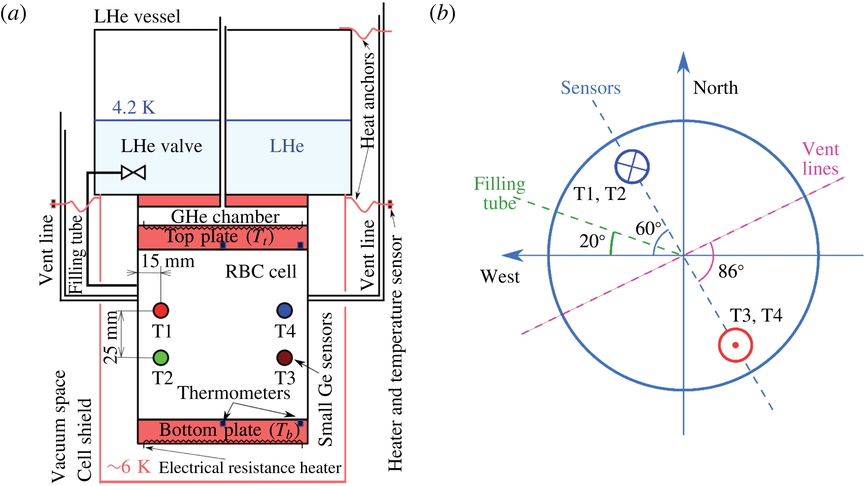
We perform our experiments in clean cryogenic environment and utilize cryogenic helium gas, representing a working fluid with well known (McCarty Reference McCarty1972; NIST 2000) and in situ tuneable properties. Our helium cryostat, described in detail by Urban et al. (Reference Urban, Hanzelka, Králík, Musilová, Skrbek and Srnka2010), is schematically shown in figure 1. In short, the convection cell is thermally connected to a liquid helium vessel (4.2 K), via a heat exchange chamber filled with gaseous helium; its main function is to remove, as uniformly as possible, the convective heat flux from the top plate. The cell and the heat exchange chamber are protected against thermal radiation by a copper shield thermally anchored to the liquid helium vessel. All internal parts of the cryostat are suspended on a central thin wall stainless steel neck in high cryogenic vacuum of order
 $10^{-6}~\text{Pa}$
.
Scheme of the apparatus. (a) Inner part of helium cryostat (Urban et al.
Reference Urban, Hanzelka, Králík, Musilová, Skrbek and Srnka2010) containing the cylindrical aspect ratio one RBC cell. Four small Ge temperature sensors (named T1–T4) measure temperature fluctuations in the fluid at opposite sides in the cell interior. Temperatures of the top (
 $T_{t}$
) and bottom (
 $T_{b}$
) plates are measured by four additional temperature sensors embedded in the centre and near the edge of both plates. The top plate temperature is stabilized. Temperature of the vent lines near the cell is controlled with electrical heaters to suppress potential effect of convection inside the lines. (b) Scheme of the azimuthal positions of vent lines, filling tube and sensors in the cell with respect to the cardinal points as seen from top. Small red and blue circles show the prevailing flow direction (warm and cold stream, respectively) observed with the sensors.

The cylindrical experimental cell with the height
 $L=0.3~\text{m}$
and diameter
 $D=0.3~\text{m}$
has been designed with particular effort to minimize the influence of its structure and materials on the observed RBC flow (Urban et al.
Reference Urban, Hanzelka, Králík, Musilová, Skrbek and Srnka2010). The cell withstands pressures of up to 3.5 bar in order to cover the range
 $10^{6}<Ra<10^{15}$
with sufficient precision of the measurements. The plates are made of 28 mm thick annealed OFHC (oxygen-free high conductivity) copper of very high thermal conductivity (at least
 $2~\text{kW}~\text{m}^{-1}~\text{K}^{-1}$
at 5 K). Design of the heaters glued in the spiral grooves milled on the external sides of plates ensures better than 1 mK temperature homogeneity of the internal side of the plates, and in the case of the top plate also assuming that the heat is uniformly removed by the exchange chamber. In the experiments, the temperature of the top plate is approximately set by adjusting the pressure in the heat exchange chamber and stabilized precisely by the heater using the Lake Shore 340 temperature controller. The parasitic heat fluxes associated with the finite thermal conductivity of sidewalls are minimized by using very thin (
 $\unicode[STIX]{x1D6FF}=0.5~\text{mm}$
at the boundary layers and
 $\unicode[STIX]{x1D6FF}=1~\text{mm}$
at the central part) stainless steel of low thermal conductivity, as well as by employing a special design of the cell corners (Urban et al.
Reference Urban, Hanzelka, Králík, Musilová, Skrbek and Srnka2010).
Temperature fluctuations inside the fluid volume are monitored using four small Ge sensors (
 $250~\unicode[STIX]{x03BC}\text{m}$
cubes, type TTR-G, Mitin et al.
Reference Mitin, McDonald, Pavese, Boltovets, Kholevchuk, Nemish, Basanets, Dugaev, Sorokin and Konakova2007; Mitin, Kholevchuk & Kolodych Reference Mitin, Kholevchuk and Kolodych2011), placed in two pairs at opposite sides near the mid-height of the cell, 1.5 cm from the sidewall and 2.5 cm vertically apart, see figure 1(a). Each sensor (typically of resistance
 $6~\text{k}\unicode[STIX]{x03A9}$
and sensitivity
 $\simeq 1~\text{k}\unicode[STIX]{x03A9}~\text{K}^{-1}$
) is a component of its own impedance bridge (Wheatstone bridge analogue), with both the sensor resistivity and parasitic capacity of its cabling balanced. The temperature fluctuations are evaluated from the voltage signal across the particular compensated bridge by the phase sensitive (lock-in) amplifier Stanford Research Systems SRS830 and recorded by PC via GPIB-USB (National Instruments) interface. The sampling of the four simultaneously measured signals is synchronized using a special data transfer mode (FAST) of the SR830 and a trigger signal of the external generator (Velleman).
Temperatures at the top (
 $T_{t}$
) and bottom (
 $T_{b}$
) plates are measured by additional four Lake Shore GR-200A-1500-1.4B germanium temperature sensors (calibrated with 5 mK uncertainty to the ITS-90 International Temperature Scale by the manufacturer) embedded in the centre and near the edge of both Cu plates. We made an additional calibration of the sensors which allows us to measure
 $\unicode[STIX]{x0394}T=T_{b}-T_{b}$
with uncertainty up to 2 mK (Urban et al.
Reference Urban, Hanzelka, Králík, Musilová, Skrbek and Srnka2010). The pressure in the cell is measured with MKS Baratron 690A (calibration traceable to NIST) with 0.08 % reading accuracy.
2.2 Data acquisition and processing
Two series of data, labelled ‘c’ and ‘d’, have been obtained in two independent experimental runs, with the cryostat and the experimental cell dismantled in between. The ‘c’ data contain records from one sensor (T4 only), obtained at
 $10^{11}\leqslant \mathit{Ra}\leqslant 3\times 10^{14}$
during the experiment focused on heat transfer efficiency measurement aimed at the maximum
 $\mathit{Ra}$
values (Urban et al.
Reference Urban, Musilová and Skrbek2011, Reference Urban, Hanzelka, Králík, Musilová, Srnka and Skrbek2012, Reference Urban, Hanzelka, Musilová, Králík, La Mantia, Srnka and Skrbek2014). The sampling frequency is 32 Hz and the lock-in amplifier integration time is 100 ms. Typical length of one record is an hour. The quality of the signal recorded is slightly affected by parasitic capacitances due to the sensor cabling which could not have been fully balanced in the bridge circuit used in this experiment. Thus the signal to noise ratio is only moderately high, of the order of 10, and decreases towards the highest values of
 $\mathit{Ra}$
. The ‘d’ data consist of synchronous records of temperature signals of four sensors (T1–T4, see figure 1) obtained for
 $10^{8}\leqslant \mathit{Ra}\leqslant 3\times 10^{13}$
. We typically apply a sampling frequency of 32 Hz or higher (up to 80 Hz), with lock-in amplifier integration times being 100 ms (300 ms in few cases). The lengths of individual records range from 1 to 47 h. The signal to noise ratio is 100 times larger in comparison with the ‘c’ data and, additionally, the linear trend of the recorded signal is numerically suppressed.
The dynamic RBC parameters are calculated based on the fluid properties evaluated at the mean temperature
 $T_{m}=(T_{b}+T_{t})/2$
in a conventional way, i.e.
 $\mathit{Ra}=g(\unicode[STIX]{x1D6FC}/\unicode[STIX]{x1D708}\unicode[STIX]{x1D705})(T_{b}-T_{t})L^{3}$
, (where
 $\unicode[STIX]{x0394}T=(T_{b}-T_{t})$
is corrected with respect to the adiabatic gradient) and
 $\mathit{Pr}=\unicode[STIX]{x1D708}/\unicode[STIX]{x1D705}$
. For subsequent statistical analysis, the raw data are processed in the following way: each raw data record, denoted
 $R(t)$
, sampled at frequency
 $f$
, consists of
 $N$
points, where the
 $i$
th signal value is recorded at
 $t=i/f$
. The signal mean
 $R_{m}$
is obtained as
 $$\begin{eqnarray}R_{m}=\frac{1}{N}\mathop{\sum }_{i=1}^{N}R(t)=\frac{1}{N}\mathop{\sum }_{i=1}^{N}R\left(\frac{i}{f}\right),\end{eqnarray}$$
while its standard deviation
 $R_{sd}$
is calculated as
 $$\begin{eqnarray}R_{sd}=\sqrt{\frac{1}{N}\mathop{\sum }_{i=1}^{N}\left[R\left(\frac{i}{f}\right)-R_{m}\right]^{2}}.\end{eqnarray}$$
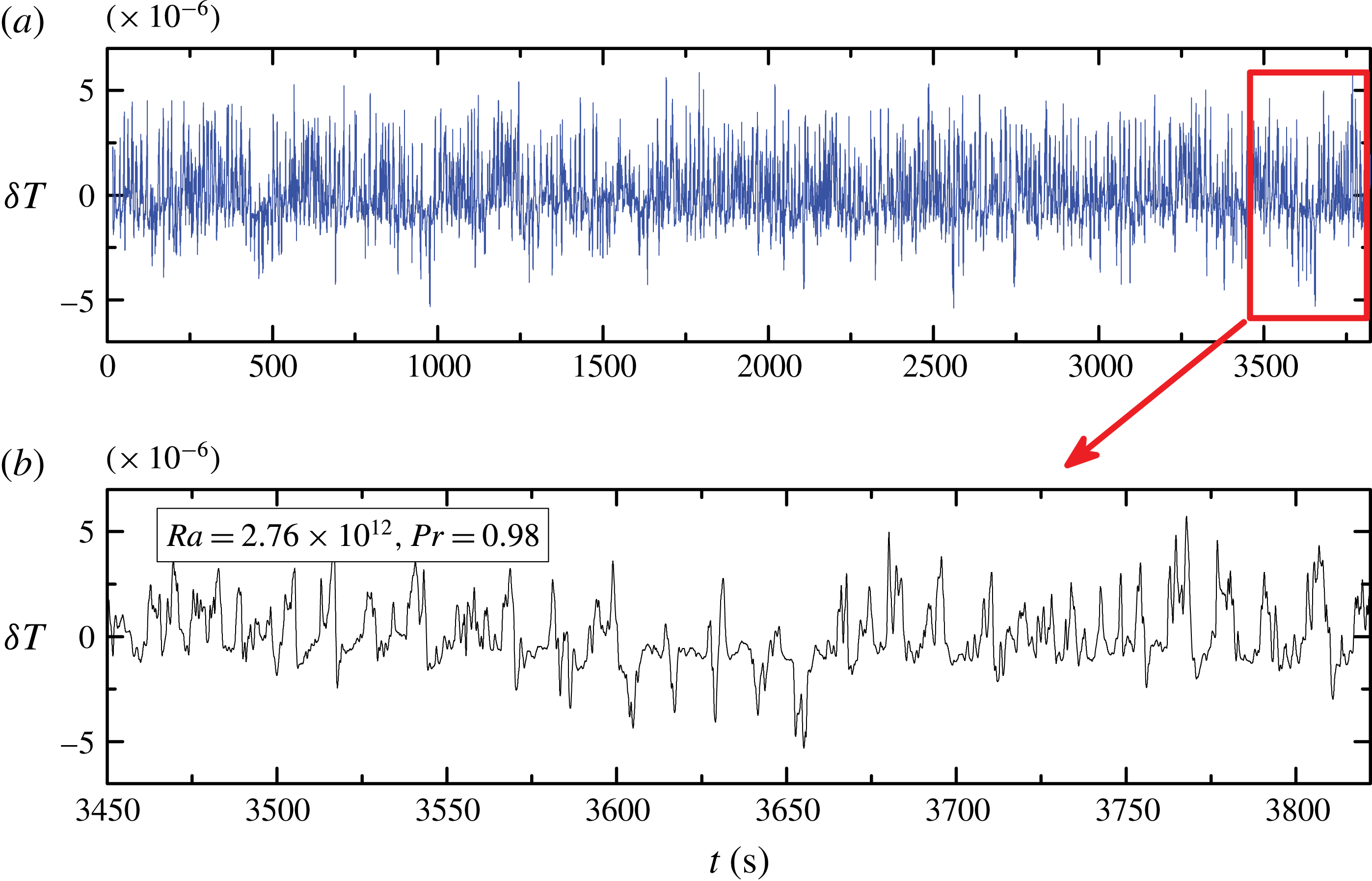
An example of the raw data records from one of the sensors (T3) can be seen in figure 2. The normalized signal
 $S_{r}(t)$
at sensor position
 $r$
is consequently defined as
 $$\begin{eqnarray}S_{r}(t)=\frac{R(t)-R_{m}}{R_{sd}}=S_{r}\left(\frac{i}{f}\right)=\frac{R(i/f)-R_{m}}{R_{sd}}.\end{eqnarray}$$
Cross-correlation functions
 $CC_{r,s}(\unicode[STIX]{x1D70F})$
of the signals detected at sensor positions
 $r$
,
 $s$
are then defined as
 $$\begin{eqnarray}CC_{r,s}(\unicode[STIX]{x1D70F})=\frac{1}{N-|m|}\mathop{\sum }_{i}S_{r}(t+\unicode[STIX]{x1D70F})S_{s}(t)=\frac{1}{N-|m|}\mathop{\sum }_{i}S_{r}\left(\frac{i+m}{f}\right)S_{s}\left(\frac{i}{f}\right),\end{eqnarray}$$
where the time delay
 $\unicode[STIX]{x1D70F}=m/f$
,
 $-N<m<N$
, and the summation index
 $i$
meets contemporaneous conditions
 $1\leqslant i\leqslant N$
and
 $1\leqslant i+m\leqslant N$
. Auto-correlation functions
 $AC_{r}(\unicode[STIX]{x1D70F})$
at the sensor
 $r$
are obtained from (2.4) simply by putting
 $r=s$
, so that
 $AC_{r}(\unicode[STIX]{x1D70F})=CC_{r,r}(\unicode[STIX]{x1D70F})$
. Typical examples of AC and CC functions can be seen in figure 7(a) below. A further useful characteristic of the signal is the power spectrum
 $S_{r}(f)$
, defined in a standard way by the square of the Fourier transform of
 $S_{r}(t)$
.
Temperature fluctuations (in arbitrary units) recorded using sensor T3 (a). Panel (b) zooms into a detail of the time record. We can see here a typical short-time reversal of the temperature spikes, i.e. sign changes of the large fluctuation bunches with respect to the mean signal
 $R_{m}$
, from prevalent (for T3) positive deviations to negative deviations (see time period between
 $t=3600$
and 3670). These were detected at all investigated
 $\mathit{Ra}$
, with an overall occurrence of approximately 10 % of time.

3 Results
3.1 Probability distribution functions of temperature fluctuations
Temperature records (see example in figure 2) contain characteristic bunches of large-
 $|\unicode[STIX]{x1D6FF}T|$
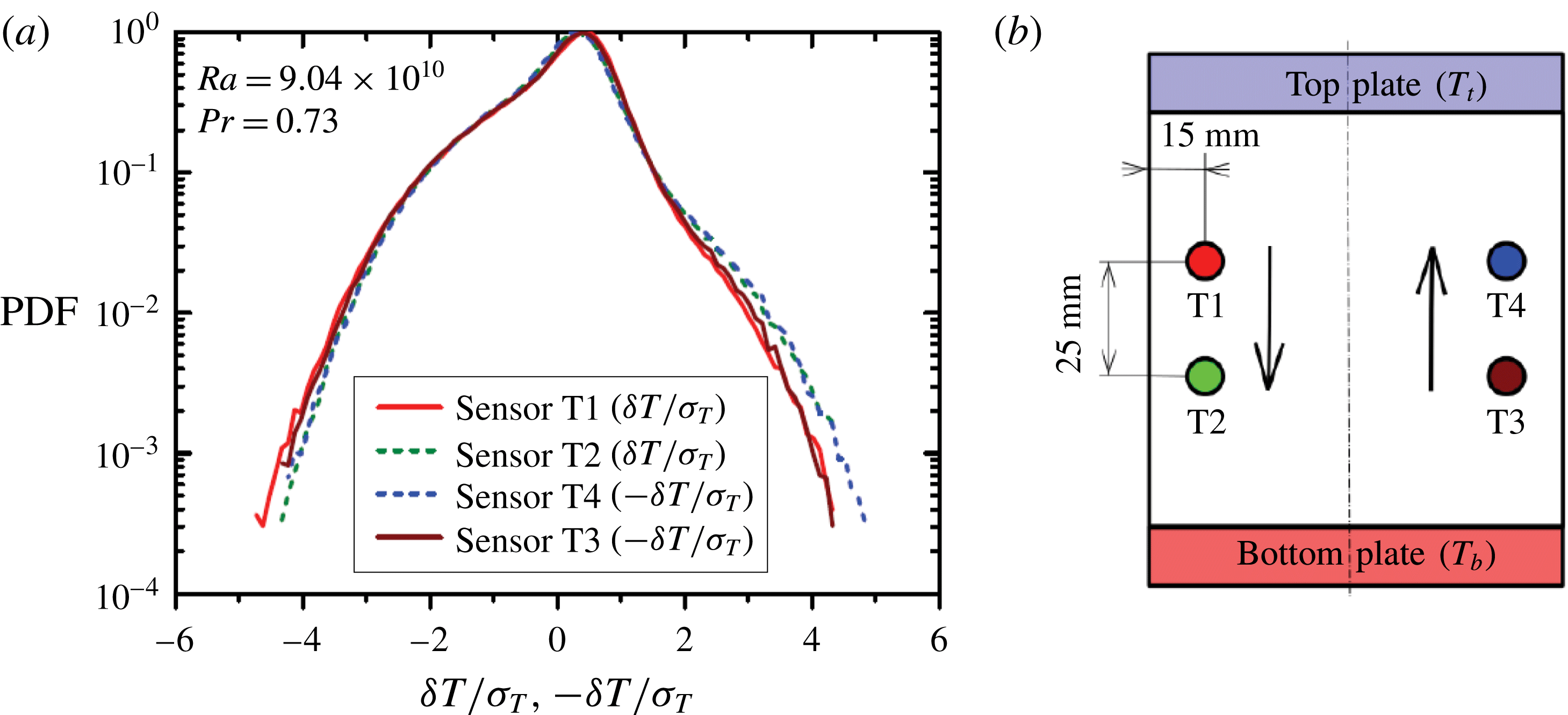
spikes, oriented most of the time towards low temperature at sensors T1 and T2 and towards high temperature at sensors T3 and T4 at the opposite side of the container, as indicated by arrows in figure 3(b). High temperature of the spike bunches at sensors T3 and T4 corresponds to an upward orientation of the mean velocity here, which we deduce from the time delay between signals, read from the cross-correlation function of temperature records, cf. figure 8 below in § 3.2. Similarly, the prevailing low temperature spikes at sensors T1 and T2 correspond to downward velocity. This type of correlation suggests that the LSC rotates prevalently in the direction from the T1 sensor towards the T2–T4 sensors. Occasional signal reversals, i.e. sign changes of the large fluctuation bunches with respect to the mean signal
 $R_{m}$
, were detected at all investigated
 $\mathit{Ra}$
, see figure 2.
(a) Probability density functions (PDFs) of temperature fluctuations
 $\unicode[STIX]{x1D6FF}T$
as measured by all sensors. The sensor positions are shown in (b) together with the prevailing LSC direction. PDFs obtained with the sensors at opposite side of the RBC cell display opposite skewness (T1, T2 versus T3, T4), so we reversed the temperature scale in the PDF plots for T3 and T4 to highlight the symmetry.
 $\unicode[STIX]{x1D70E}_{T}$
stands for the standard temperature deviation. Slight difference between PDFs of the leading sensors (T1 and T3), facing the LSC flow on one hand, and the trailing sensors (T2 and T4) on the other hand can be seen, while members of each pair show mutually almost identical PDFs.

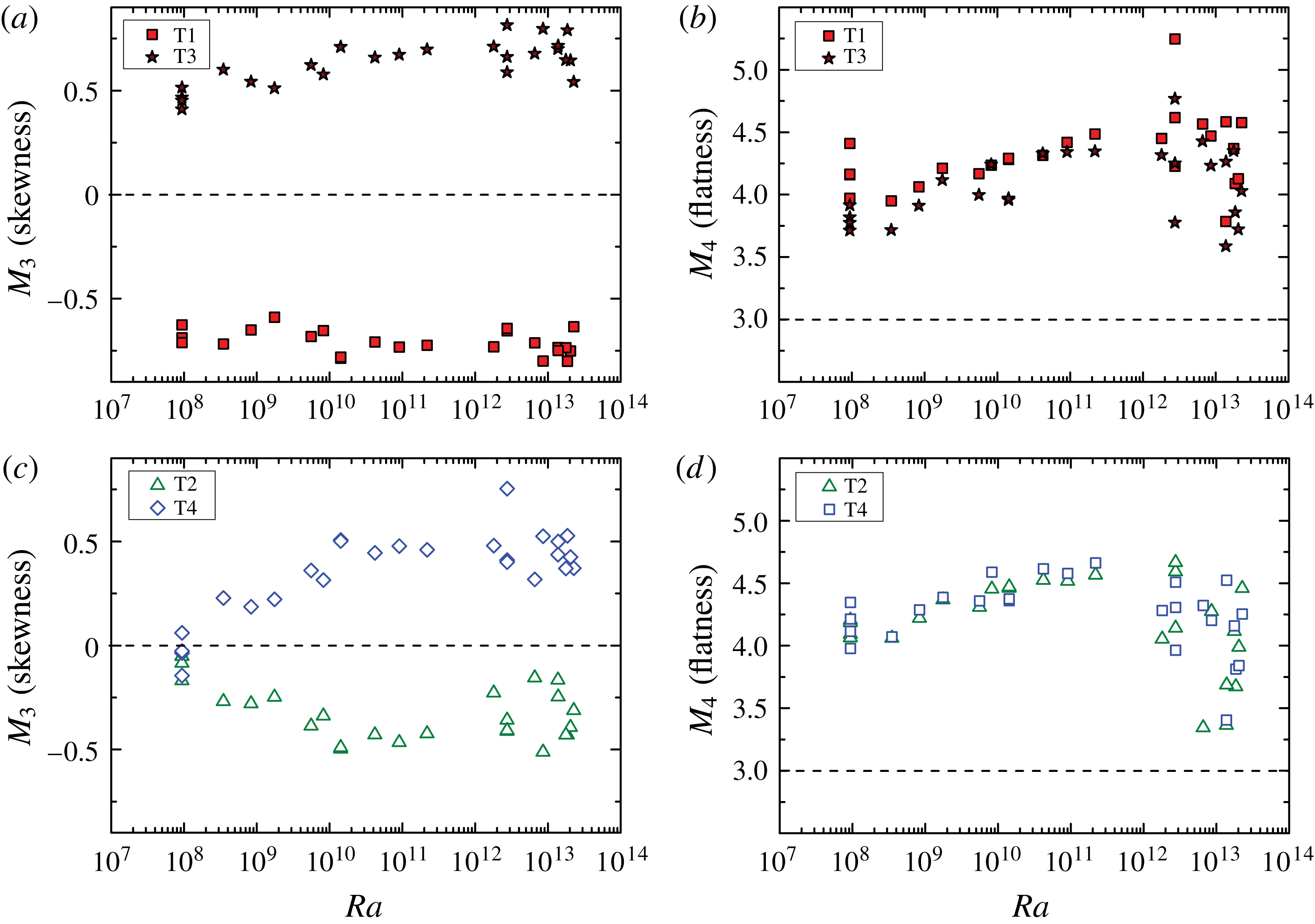
Skewness (
 $M_{3}$
) and flatness (
 $M_{4}$
) of temperature fluctuation PDFs. Sensors T1 and T3 are the ‘leading sensors’ facing the mean LSC flow, while T2 and T4 are ‘hidden’ behind them, and are thus called ‘trailing sensors’. The values at high end of
 $\mathit{Ra}>10^{12}$
are influenced by lower signal to noise ratio of temperature signals in the experimental run ‘c’.

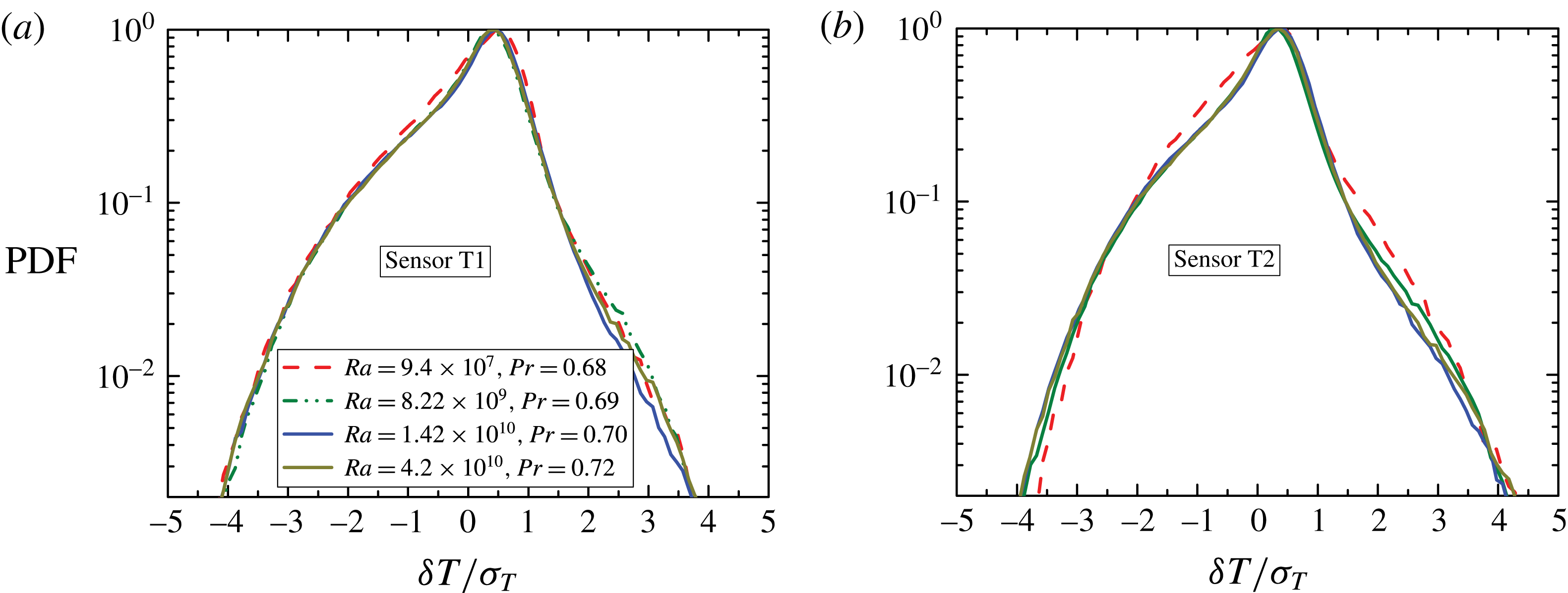
Temperature fluctuation PDFs recorded for various
 $\mathit{Ra}$
compared between leading (a) and trailing sensors (b). Data from T1 and T2 are shown. Notice the relatively lower skewness of the trailing sensor PDF at the lowest value of
 $\mathit{Ra}$
, clearly distinct from the same sensor PDF at high
 $\mathit{Ra}$
and all the leading sensor PDFs, which depend on
 $\mathit{Ra}$
only weakly, in particular their skewness is practically constant (cf. figure 4).

Figure 3(a) shows typical examples of probability density functions (PDFs) for normalized temperature fluctuations seen at all four sensors at
 $\mathit{Ra}\gtrsim 10^{10}$
. For the T3 and T4 sensors, the PDFs are plotted with respect to
 $-\unicode[STIX]{x1D6FF}T/\unicode[STIX]{x1D70E}_{T}$
, in order to illustrate the similarity in shapes. At sensors T3 and T4, the higher shoulders of PDFs at higher temperatures correspond to the prevailing rising warm fluid structures; the skewness (the third moment
 $M_{3}$
of the PDF) is positive here. At sensors T1 and T2, a similar but opposite situation occurs, where the higher PDF shoulders at low temperatures reflect the descending cool flow structures, and result in negative skewness
 $M_{3}<0$
.
Looking at the evolution of PDFs with
 $\mathit{Ra}$
in more detail, we see differences between PDFs corresponding to the ‘leading sensors’, facing the flow (T1 and T3), and the ‘trailing sensors’ (T2 and T4), being most apparent in the skewness
 $M_{3}$
. First, the absolute value of
 $M_{3}$
is larger for the former than for the latter (figure 4
a,c). Second, and more important,
 $M_{3}$
breaks for the trailing sensors at approximately
 $\mathit{Ra}\sim 10^{10}$
from a roughly linear rise (in absolute value) starting from
 $|M_{3}|\approx 0$
, seen at smaller values of
 $\mathit{Ra}$
, to a value saturated around
 $|M_{3}|\approx 0.5$
for higher
 $\mathit{Ra}$
. Figure 5 shows examples of the PDFs corresponding to the low-
 $\mathit{Ra}$
(‘growing skewness’) regime and the high-
 $\mathit{Ra}$
(‘saturated skewness’) regime for one of the leading sensors (a), where the differences are marginal, and for a trailing sensor (b), where the PDF is considerably more symmetric at the low
 $\mathit{Ra}=9.4\times 10^{7}$
(
 $|M_{3}|\approx 0.15$
), than at the high
 $\mathit{Ra}=4.2\times 10^{10}$
(
 $|M_{3}|\approx 0.5$
). At
 $\mathit{Ra}\gtrsim 10^{10}$
, the skewness at the trailing sensors remains still slightly lower compared to the leading sensors, which is related to small difference between the tails of the PDFs, pronounced mainly on the lower-shoulder side, as seen in figure 5. This corresponds to streamwise smearing of the fluctuations (mainly due to decreasing temperature contrast of plumes) away from the top and bottom plates. Concerning the fourth PDF moment (
 $M_{4}$
) – the flatness – the leading sensors display slightly lower values of
 $M_{4}$
compared to the trailing sensors, see figure 4(b,d), however no apparent changes in the scaling are seen, in contrast to the behaviour of
 $M_{3}$
.
The above behaviour of the PDF skewness can be interpreted in line with the suggestion of Niemela & Sreenivasan (Reference Niemela and Sreenivasan2003b
) (indirect interpretation of a helium experiment) and the measurements of Sun et al. (Reference Sun, Xia and Tong2005) (direct PIV visualization in water) as a transition in shape of the LSC from an elongated ellipse or oval positioned diagonally across the cell to a more extended squarish or round shape: as the PDF skewness is low in absolute value for the trailing sensors for
 $\mathit{Ra}$
below
 ${\sim}10^{10}$
, we can infer that these sensors are lying further outside of the main LSC flow for
 $\mathit{Ra}<10^{10}$
. Simultaneously, the position of the leading sensors with respect to the main flow remains apparently unchanged for all considered
 $\mathit{Ra}$
values, as the respective skewness is practically constant. Such a situation presumably corresponds to the elongated shape of the LSC. With increasing
 $\mathit{Ra}$
, the LSC flow gradually embraces also the trailing sensors, until their skewness saturates at
 $\mathit{Ra}\sim 10^{10}$
, corresponding to the new shape of the LSC, approaching all the cell walls more evenly.
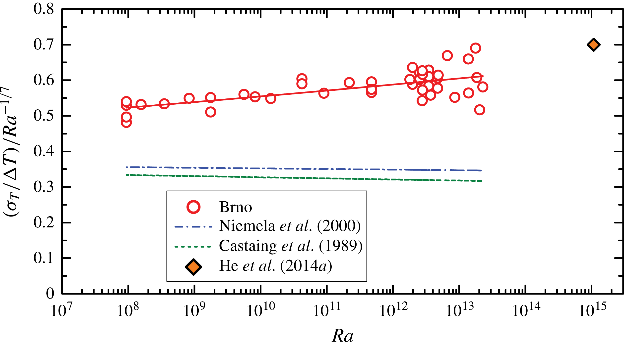
Finally, in figure 6, we show the standard deviations normalized by the overall temperature drop
 $\unicode[STIX]{x0394}T$
between the top and bottom plates. We detect a uniform scaling
 $\langle \unicode[STIX]{x1D6FF}T/\unicode[STIX]{x0394}T\rangle =(0.41\pm 0.02)\times Ra^{-0.130\pm 0.002}$
within
 $10^{8}\leqslant \mathit{Ra}\leqslant 3\times 10^{13}$
. Notice that the exponent is steeper than the
 $\mathit{Ra}^{-1/7}$
scaling as well as the cryogenic helium results of Castaing et al. (Reference Castaing, Gunaratne, Heslot, Kadanoff, Libchaber, Thomae, Wu, Zaleski and Zanetti1989), performed midway between the sidewall and the cell centre, and Niemela et al. (Reference Niemela, Skrbek, Sreenivasan and Donnelly2000), measured in the cell centre. Also the overall amplitude is approximately
 $2\times$
higher in our experiment. Both facts are related to the sensor position near the sidewall. This is supported by the comparison with the data point by He et al. (Reference He, van Gils, Bodenschatz and Ahlers2014a
), measured in a pressurized
 $SF_{6}$
 $\unicode[STIX]{x1D6E4}=1/2$
cell at
 $\mathit{Ra}=1.08\times 10^{15};\mathit{Pr}=0.8$
at the mid-height of the cell at three points near the sidewall, giving mutually very close results, which are consistent with our dependence.
Standard deviation of temperature fluctuations
 $\unicode[STIX]{x1D70E}_{T}/\unicode[STIX]{x0394}T$
, normalized by the temperature difference between the bottom and top plate, and compensated by
 $\mathit{Ra}^{-1/7}$
. Our data, measured near the sidewall, are compared with the results of Castaing et al. (Reference Castaing, Gunaratne, Heslot, Kadanoff, Libchaber, Thomae, Wu, Zaleski and Zanetti1989), measured midway between the sidewall and the centre and Niemela et al. (Reference Niemela, Skrbek, Sreenivasan and Donnelly2000), measured at the cell centre, and the data point by He et al. (Reference He, van Gils, Bodenschatz and Ahlers2014a
) near the wall in an
 $SF_{6}$
experiment.

3.2 Power spectra, auto-correlations and cross-correlations of temperature fluctuations
The power spectra of temperature fluctuations
 $S_{f}$
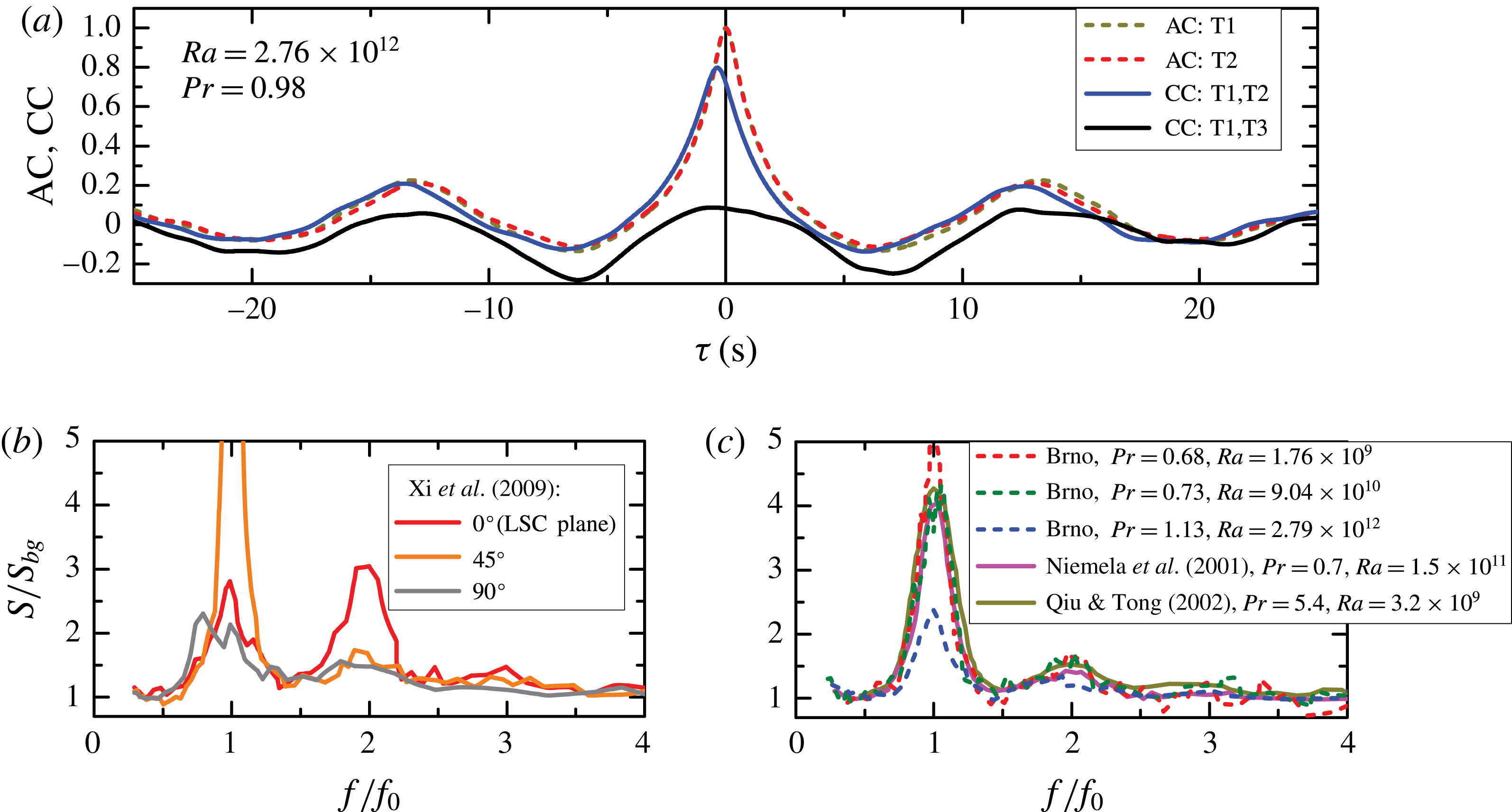
recorded in this experiment at individual sensors generally display one pronounced characteristic peak together with a weaker secondary one at twofold frequency, as can be seen in figure 7(b,c), where the data are compensated by the background temperature fluctuations’ power spectra
 $S_{bg}(f)$
. The frequency
 $f_{0}$
of the main peak corresponds to the occurrence of pronounced spike bunches in the raw temperature signal (see figure 2), with an associated time period
 $T_{0}=1/f_{0}$
. Alternatively, this period
 $T_{0}$
can be evaluated from the position of the first side maximum of the auto-correlation function (2.4) as seen in figure 7(a). The values of
 $T_{0}$
measured in our experiment range between 6 and 40 s.
(a) The auto-correlation functions (AC) together with the cross-correlation function (CC) of temperature fluctuation signals recorded by sensors at opposite sides of the RBC cell. The time
 $T_{0}$
derived from the positions of first side maxima corresponds to the main peak frequency
 $f_{0}=1/T_{0}$
in the power spectra. (b,c) Power spectra of temperature fluctuations at mid-plane near the sidewall in
 $2^{\circ }$
tilted water sample obtained by Xi et al. (Reference Xi, Zhou, Zhou, Chan and Xia2009) at azimuthal position
 $0^{\circ }$
(LSC plane) together with
 $45^{\circ }$
and
 $90^{\circ }$
from LSC plane (
 $\mathit{Pr}=5.3$
,
 $Ra=5\times 10^{9}$
) (b) and by Niemela et al. (Reference Niemela, Skrbek, Sreenivasan and Donnelly2001) (
 $\mathit{Pr}=0.8$
,
 $Ra=1.5\times 10^{11}$
), Qiu & Tong (Reference Qiu and Tong2002) (
 $\mathit{Pr}=5.5$
,
 $Ra=1.4\times 10^{9}$
) and measured by us (marked as ‘Brno’) for
 $\mathit{Pr}\sim 1$
and
 $\mathit{Ra}$
as indicated (c). Dependencies compensated with respect to the background power spectra
 $S_{bg}$
are shown.

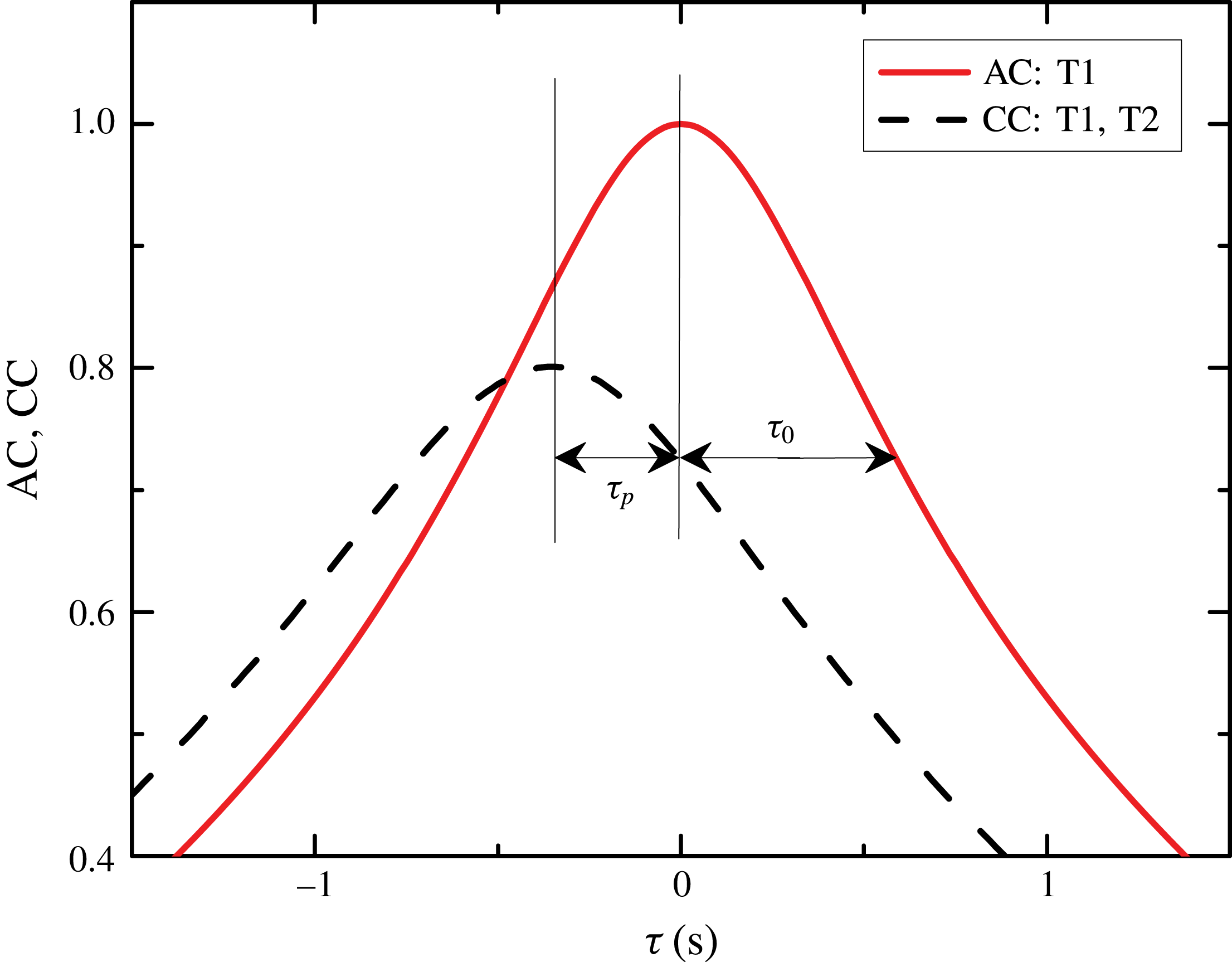
Auto-correlation function (red solid) of temperature fluctuations and cross-correlation function (black dashed) of time records at nearby sensors, distant by
 $d=2.5~\text{cm}$
. Time delays
 $\unicode[STIX]{x1D70F}_{p}$
and
 $\unicode[STIX]{x1D70F}_{0}$
define velocities
 $U_{p}$
,
 $U$
,
 $V$
and
 $U_{eff}$
used in various definitions of Reynolds number (3.2)–(3.5). Time delay
 $\unicode[STIX]{x1D70F}_{p}$
between signals at positions distant by
 $d$
relates to the Taylor hypothesis-based mean flow velocity
 $U_{p}=d/\unicode[STIX]{x1D70F}_{p}$
. The figure is a zoom into the AC and CC functions shown in figure 7(a).

The character of measured power spectra allows us to infer on the azimuthal orientation of the LSC plane, when we compare them with the azimuthally resolved spectra obtained by Xi et al. (Reference Xi, Zhou, Zhou, Chan and Xia2009) in a water sample tilted by
 $2^{\circ }$
, see figure 7(b). To highlight the proportions between the first and second peak in
 $S(f)$
, we divide the spectra by a fit to the background spectrum
 $S_{bg}(f)$
. Due to the sloshing mode, the peak of the ‘second harmonics’ in the experimental spectra of Xi et al. (Reference Xi, Zhou, Zhou, Chan and Xia2009) is found to be comparable or higher than the first peak when the sensor is in azimuthal position of the LSC plane (at
 $0^{\circ }$
). The spectra shown in figure 7(c) suggest that the position of sensors in our experiments is azimuthally turned by an angle between
 $45^{\circ }{-}90^{\circ }$
with respect to the LSC plane. While the height of the second normalized peak in our (Brno) measurements is less than one, the height of the first peak varies between 2 and 6, and no tendency with
 $\mathit{Ra}$
is observed. Thus our sensors are most probably positioned at the edge of the mean flow at all
 $\mathit{Ra}$
. We shall see in § 3.3, figure 9(d), that our measured velocity is by approximately 40 % lower than the velocity measured by He et al. (Reference He, van Gils, Bodenschatz and Ahlers2015) close to the LSC plane, which indirectly confirms previous conclusion on sensors positions. We emphasize that the sensor position does not affect the measured period
 $T_{0}$
(and frequency
 $f_{0}$
) of the bulk fluid oscillations (Brown et al.
Reference Brown, Funfschilling and Ahlers2007), and consequently the frequency-based Reynolds number, discussed below.
Further, we have evaluated two-point statistics by calculating the cross-correlations (2.4) between pairs of sensors. Figure 7(a) shows examples of CCs between a pair suspended 2.5 cm above one another (T1, T2) and a pair of sensors on the opposite sides of the cell (T1, T3). Shift of the main maximum of the CC with respect to that of the AC (i.e.
 $\unicode[STIX]{x1D70F}=0$
), and the shapes of the respective peaks, both shown in detail in figure 8, can be used to estimate the mean and fluctuating turbulent flow velocities, as discussed in the following section.
3.3 Reynolds numbers
We use several definitions of Reynolds number aiming to compare our data with results published by other authors directly. For a survey of various definitions of
 $\mathit{Re}$
depending on the method historically used for characterization of the LSC, see the review of Ahlers et al. (Reference Ahlers, Grossmann and Lohse2009). In short, in one probe measurement, the characteristic frequency
 $f_{0}=1/T_{0}$
determined from the power spectrum (or auto-correlation function) is used in definition of the frequency-based Reynolds number
 $\mathit{Re}_{f0}$
:
 $$\begin{eqnarray}\mathit{Re}_{f0}=2\frac{L^{2}f_{0}}{\unicode[STIX]{x1D708}}.\end{eqnarray}$$
In two probe measurements, the simplest approach uses the Taylor’s frozen flow hypothesis (Tritton Reference Tritton1988; Kadanoff Reference Kadanoff2001), assuming that temperature structure is not dissipated between the sensors. The time delay
 $\unicode[STIX]{x1D70F}_{p}$
between records at two nearby positions (see figure 8) spaced by a distance
 $d$
determines the velocity
 $U_{p}=d/\unicode[STIX]{x1D70F}_{p}$
. The corresponding Reynolds number is defined as
 $$\begin{eqnarray}\mathit{Re}_{p}=\frac{LU_{p}}{\unicode[STIX]{x1D708}}.\end{eqnarray}$$
Taylor’s hypothesis does not apply when velocity fluctuations are not small in comparison with the mean flow velocity. Then, a more appropriate method is the elliptic approximation, proposed for the general space–time cross-correlation function along the homogeneous flow by He & Zhang (Reference He and Zhang2006) and Zhao & He (Reference Zhao and G.-W.2009), and which has been tested in RBC by He, He & Tong (Reference He, He and Tong2010) and used frequently since. In this method, Reynolds number
 $\mathit{Re}_{U}$
is related to the mean flow velocity,
 $\mathit{Re}_{V}$
is related to velocity fluctuations and the ‘effective’
 $\mathit{Re}_{eff}$
may be defined as:
 $$\begin{eqnarray}\displaystyle & \displaystyle \mathit{Re}_{U}={\displaystyle \frac{LU}{\unicode[STIX]{x1D708}}};\quad U=d{\displaystyle \frac{\unicode[STIX]{x1D70F}_{p}}{\unicode[STIX]{x1D70F}_{0}^{2}}}=U_{p}\left({\displaystyle \frac{\unicode[STIX]{x1D70F}_{p}}{\unicode[STIX]{x1D70F}_{0}}}\right)^{2}; & \displaystyle\end{eqnarray}$$
 $$\begin{eqnarray}\displaystyle & \displaystyle \mathit{Re}_{V}={\displaystyle \frac{LV}{\unicode[STIX]{x1D708}}};\quad V={\displaystyle \frac{d}{\unicode[STIX]{x1D70F}_{0}}}\sqrt{1-\left({\displaystyle \frac{\unicode[STIX]{x1D70F}_{p}}{\unicode[STIX]{x1D70F}_{0}}}\right)^{2}}; & \displaystyle\end{eqnarray}$$
 $$\begin{eqnarray}\displaystyle & \displaystyle \mathit{Re}_{eff}=\frac{LU_{eff}}{\unicode[STIX]{x1D708}};\quad U_{eff}=\sqrt{U^{2}+V^{2}}={\displaystyle \frac{d}{\unicode[STIX]{x1D70F}_{0}}}. & \displaystyle\end{eqnarray}$$
In our experiment, recording temperature fluctuations at two nearby positioned sensors along the flow enables us to deduce both velocities
 $U$
and
 $V$
thus defining the full structure of the space–time cross-correlations. Indeed, from the auto-correlation function (supposed to be identical at both these nearby positions) and the cross-correlation function between the corresponding two records at a leading and a trailing sensor (see figure 8), we obtain the time delays
 $\unicode[STIX]{x1D70F}_{0}$
,
 $\unicode[STIX]{x1D70F}_{p}$
and, subsequently, velocities
 $U$
and
 $V$
. We obtain the values of
 $U$
and
 $V$
by fitting the elliptic model to the AC and CC curves, such as those plotted in figure 8. It is evident from the relation for fluctuation velocity
 $V$
that
 $\unicode[STIX]{x1D70F}_{0}>\unicode[STIX]{x1D70F}_{p}$
and thus
 $U_{eff}<U_{p}$
. As a result,
 $\mathit{Re}_{p}>\mathit{Re}_{eff}>\mathit{Re}_{U};\mathit{Re}_{V}$
.
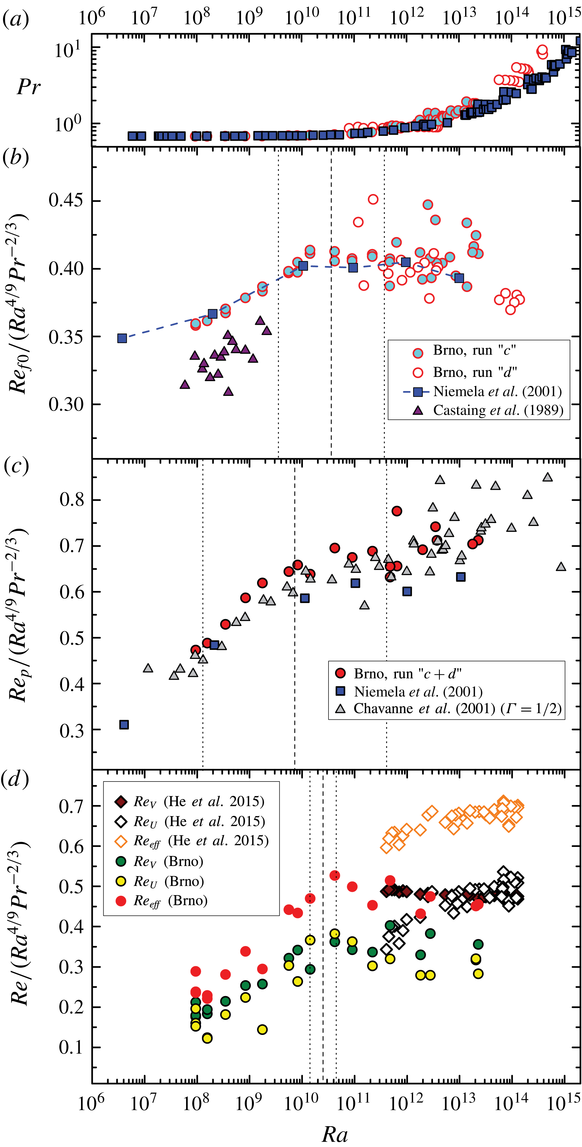
Prandtl (a) and Reynolds numbers (b–d) in cryogenic helium and pressurized
 $SF_{6}$
experiments: our results (Brno) are compared with data obtained in the aspect ratio one cell of Castaing et al. (Reference Castaing, Gunaratne, Heslot, Kadanoff, Libchaber, Thomae, Wu, Zaleski and Zanetti1989), Niemela et al. (Reference Niemela, Skrbek, Sreenivasan and Donnelly2001), He et al. (Reference He, van Gils, Bodenschatz and Ahlers2015) and aspect ratio
 $1/2$
of Chavanne et al. (Reference Chavanne, Chilla, Chabaud, Castaing and Hebral2001). The Reynolds numbers
 $\mathit{Re}_{f0}$
(3.1),
 $\mathit{Re}_{p}$
(3.2) and the elliptic method based
 $\mathit{Re}_{U},\mathit{Re}_{V}$
and
 $\mathit{Re}_{eff}$
(3.3)–(3.5) are all compensated by the
 ${\sim}\mathit{Ra}^{4/9}\mathit{Pr}^{-2/3}$
dependence. The vertical lines indicate the values of
 $Ra_{c}$
(dashed) and the corresponding transition intervals (dotted) for
 $Re_{f0}$
,
 $Re_{p}$
and
 $Re_{eff}$
(see text and table 1).

In figure 9, we present the one-point and two-point Reynolds numbers
 $\mathit{Re}_{f0}$
, and
 $\mathit{Re}_{p}$
,
 $\mathit{Re}_{U}$
,
 $\mathit{Re}_{V}$
,
 $\mathit{Re}_{eff}$
determined from our data (labelled ‘Brno’) and compare them with results of other cryogenic experiments (with gaseous helium as working fluid) performed for
 $10^{6}<\mathit{Ra}<10^{14}$
in cylindrical
 $\unicode[STIX]{x1D6E4}=1$
(Castaing et al.
Reference Castaing, Gunaratne, Heslot, Kadanoff, Libchaber, Thomae, Wu, Zaleski and Zanetti1989; Niemela et al.
Reference Niemela, Skrbek, Sreenivasan and Donnelly2001) and
 $\unicode[STIX]{x1D6E4}=1/2$
(Chavanne et al.
Reference Chavanne, Chilla, Chabaud, Castaing and Hebral2001) RBC cells and with the data of He et al. (Reference He, van Gils, Bodenschatz and Ahlers2015) obtained with pressurized
 $SF_{6}$
. (Note that both fluids should behave similarly for approximately
 $\mathit{Ra}<10^{13}$
, due to their very similar values of
 $\mathit{Pr}$
in this range of
 $\mathit{Ra}$
. In particular, according to the original parametrizations of the GL theory (Grossmann & Lohse Reference Grossmann and Lohse2001, Reference Grossmann and Lohse2002), they should undergo the
 $IV_{l}{-}IV_{u}$
transition at
 $\mathit{Ra}\sim 10^{10}$
, see also below.) We utilize here one of the theoretically predicted (Grossmann & Lohse Reference Grossmann and Lohse2000, Reference Grossmann and Lohse2001, Reference Grossmann and Lohse2002, Reference Grossmann and Lohse2004) scalings
 $\mathit{Re}\sim \mathit{Ra}^{4/9}\mathit{Pr}^{-2/3}$
, and display the data in a compensated form. This is useful especially in order to compare the data at higher
 $\mathit{Ra}$
, where the Prandtl numbers
 $\mathit{Pr}$
in our own and the other experiments differ. In all considered experiments, the temperature probes were positioned at middle height and near the sidewall (Niemela et al.
Reference Niemela, Skrbek, Sreenivasan and Donnelly2001, Brno) or midway of the cell radius (Castaing et al.
Reference Castaing, Gunaratne, Heslot, Kadanoff, Libchaber, Thomae, Wu, Zaleski and Zanetti1989; Chavanne et al.
Reference Chavanne, Chilla, Chabaud, Castaing and Hebral2001). Values of
 $\mathit{Re}_{U}$
,
 $\mathit{Re}_{V}$
and
 $\mathit{Re}_{eff}$
were not evaluated in the older experiments (Castaing et al.
Reference Castaing, Gunaratne, Heslot, Kadanoff, Libchaber, Thomae, Wu, Zaleski and Zanetti1989; Chavanne et al.
Reference Chavanne, Chilla, Chabaud, Castaing and Hebral2001; Niemela et al.
Reference Niemela, Skrbek, Sreenivasan and Donnelly2001; Niemela & Sreenivasan Reference Niemela and Sreenivasan2003a
), and we are thus restricted to comparisons of
 $\mathit{Re}_{f0}$
and
 $\mathit{Re}_{p}$
.
Looking at the cryogenic helium data shown in figure 9 in detail, we notice that the differences in scalings are visible for
 $\mathit{Ra}<10^{10}$
. Here, having
 $\mathit{Pr}=0.686\pm 0.007$
, the scaling of the frequency number
 $\mathit{Re}_{f0}\propto \mathit{Ra}^{0.47}$
(see b) is less steep than that of all the velocity numbers
 $\mathit{Re}_{p}\propto \mathit{Ra}^{0.52}$
(c) and also
 $\mathit{Re}_{U}$
,
 $\mathit{Re}_{V}$
,
 $\mathit{Re}_{eff}$
(d). In contrast, for
 $\mathit{Ra}>10^{10}$
(where
 $\mathit{Pr}$
varies from 0.7 to 10) scalings of both types of Reynolds numbers converge and are consistent with
 $\mathit{Re}\propto \mathit{Ra}^{4/9}\mathit{Pr}^{-2/3}$
. The prefactors
 $\unicode[STIX]{x1D709}$
depend on the
 $\mathit{Re}$
definition,
 $\unicode[STIX]{x1D709}=0.40$
for
 $\mathit{Re}_{f0}$
, from 0.6 to 0.7 for
 $\mathit{Re}_{p}$
and from 0.3 to 0.4 for
 $\mathit{Re}_{U}$
and
 $\mathit{Re}_{V}$
.
To capture the above changes in scaling of
 $Re$
more quantitatively, we searched for an optimal fit of our data by two power laws of the form
 $Re\propto Ra^{\unicode[STIX]{x1D701}}Pr^{-2/3}$
, where we assumed a simple power law dependence on
 $Pr$
, and twofold dependence on
 $Ra$
with
 $\unicode[STIX]{x1D701}=\unicode[STIX]{x1D701}_{L}$
or
 $\unicode[STIX]{x1D701}_{R}$
. (The
 $Re\propto Pr^{-2/3}$
scaling was chosen in accord with the scaling determined from our data at
 $Ra>10^{11}$
within the experimental
 $Ra{-}Pr$
space for the frequency Reynolds number, yielding
 $Re_{f0}\propto Ra^{0.437}\times Pr^{-0.675}$
, as well as applying the GL model (Grossmann & Lohse Reference Grossmann and Lohse2001, Reference Grossmann and Lohse2002; Stevens et al.
Reference Stevens, van der Poel, Grossmann and Lohse2013) to our data, yielding similarly
 $Re\propto Ra^{0.442}\times Pr^{-0.666}$
.) In case of each Reynolds number type, we split the data into two disjoint sets (denoted
 $L$
,
 $R$
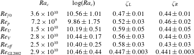
), with the optimum splitting determined by the minimal sum of squared errors for the two fits combined. Intersection of these two fits provided us with the critical points
 $Ra_{c}$
of the transition, demarcated in each panel by the dashed vertical lines. The ‘error of the critical point’, or better the ‘transitional interval’, was obtained by similar intersections of alternative fits, corresponding to bounds of the 95 % confidence level intervals for the respective fit parameters. The results are indicated by vertical lines in figure 9 and summarized in table 1 together with the exponents
 $\unicode[STIX]{x1D701}=\unicode[STIX]{x1D701}_{L}$
and
 $\unicode[STIX]{x1D701}=\unicode[STIX]{x1D701}_{R}$
. We can see that the interval for
 $Re_{p}$
in (c) is very wide, reflecting the not too pronounced change of scaling seen, when assuming the Taylor hypothesis of frozen fluctuations. In contrast, the
 $Re$
numbers determined by the more advanced elliptic approximation show a much sharper transition, with the interval corresponding to
 $Re_{eff}$
spanning less than a decade, which is comparable to the interval obtained by the same method for the theoretical curve of the GL theory (the original Grossmann & Lohse Reference Grossmann and Lohse2001, Reference Grossmann and Lohse2002 fit), and slightly narrower than the interval for
 $Re_{f0}$
, which spans approximately two decades in
 $Ra$
. The transitional intervals determined here are affected by both the experimental errors of our data, as well as fundamentally by the character of the
 $Re(Ra)$
dependencies deviating from pure power laws (Grossmann & Lohse Reference Grossmann and Lohse2000, Reference Grossmann and Lohse2001, Reference Grossmann and Lohse2002, Reference Grossmann and Lohse2004). Within the precision of the current data, the critical points of the different
 $Re$
numbers are mutually compatible, and we conclude that the transition takes place approximately between
 $Ra\sim 10^{10}{-}10^{11}$
.
In general, the Prandtl number in cryogenic experiments is fairly constant (
 $0.7<\mathit{Pr}<1$
) up to
 $\mathit{Ra}\sim 10^{12}$
(see figure 9
a). We can notice a very good agreement between
 $\mathit{Re}_{f0}$
(b) and
 $\mathit{Re}_{p}$
(c) from our experiment with the data of Chavanne et al. (Reference Chavanne, Chilla, Chabaud, Castaing and Hebral2001) and Niemela et al. (Reference Niemela, Skrbek, Sreenivasan and Donnelly2001), especially within the region of nearly constant
 $\mathit{Pr}\simeq 0.7$
, up to
 $\mathit{Ra}\sim 10^{11}$
. The comparison of our (cryogenic helium) and Göttingen data (obtained with
 $SF_{6}$
in a considerably larger cell at the same absolute distance of the sensors from the sidewall) on
 $\mathit{Re}_{U}$
,
 $\mathit{Re}_{V}$
and
 $\mathit{Re}_{eff}$
in figure 9(d) shows some differences: We see that over the
 $\mathit{Ra}$
domain of overlap, the Göttingen data lay by approximately 40 % higher, which is in qualitative agreement with the fact that our sensors are azimuthally shifted from the LSC plane, see § 3.2. Additionally, the Göttingen data display distinctly different scaling of
 $\mathit{Re}_{U}$
and
 $\mathit{Re}_{V}$
, while our data seem to show similar scaling for both of these quantities. We do not see a clear explanation, and apparently, further dedicated experiments are needed to fully resolve this issue.
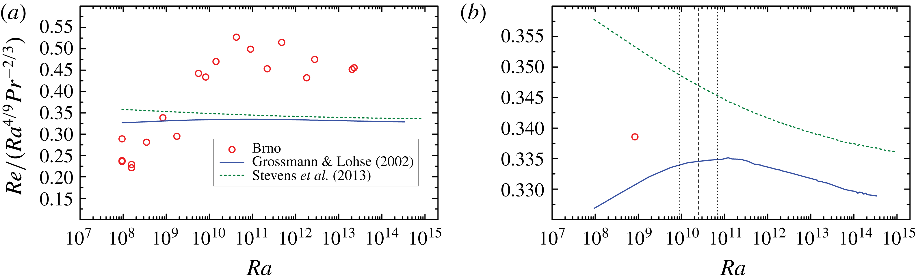
Comparison of our experimental values of
 $\mathit{Re}_{eff}$
with the Grossmann–Lohse theory in the original (Grossmann & Lohse Reference Grossmann and Lohse2001, Reference Grossmann and Lohse2002) and the updated (Stevens et al.
Reference Stevens, van der Poel, Grossmann and Lohse2013) fits. The zoom-in, shown in (b) traces in detail the change of scaling associated with the
 $IV_{l}$
–
 $IV_{u}$
transition predicted for helium data by the original fit, while no transition is seen in the updated fit, as it places the helium data fully into the
 $IV_{u}$
region in this
 $\mathit{Ra}$
range, cf. Stevens et al. (Reference Stevens, van der Poel, Grossmann and Lohse2013). The vertical lines in (b) relate to the Grossmann & Lohse (Reference Grossmann and Lohse2002) curve, and their meaning is as in figure 9.

Transitional values of
 $Ra_{c}$
for different types of Reynolds numbers with the scaling exponents
 $\unicode[STIX]{x1D701}=\unicode[STIX]{x1D701}_{L}$
corresponding to
 $Ra<Ra_{c}$
and
 $\unicode[STIX]{x1D701}=\unicode[STIX]{x1D701}_{R}$
corresponding to
 $Ra>Ra_{c}$
. The Prandtl number dependence is assumed to be
 $Re\propto Pr^{-2/3}$
(see text).

Let us now compare the experimental
 $\mathit{Re}(\mathit{Ra})$
dependencies with those obtained from the theory of Grossmann and Lohse. The calculations for our values of
 $\mathit{Ra},\mathit{Pr}$
using both the original fit of the GL model (Grossmann & Lohse Reference Grossmann and Lohse2001, Reference Grossmann and Lohse2002) and the updated version (Stevens et al.
Reference Stevens, van der Poel, Grossmann and Lohse2013) are shown in figure 10(a) together with our data for
 $\mathit{Re}_{eff}$
. We can immediately notice that both theoretical curves, in contrast to the data, show only a relatively weak dependence on
 $\mathit{Ra}$
. Zooming into the theoretical dependencies (b), different behaviours of the two curves can be seen: the GL model in the original parametrization shows the
 $IV_{l}{-}IV_{u}$
(a cross-over between the viscous and thermal boundary layers) transition at
 $\mathit{Ra}\sim 10^{10}{-}10^{11}$
(cf. table 1) accompanied by a change of
 $\mathit{Re}(\mathit{Ra})$
scaling from a steeper to a flatter, qualitatively corresponding to the data, however being much less pronounced. On the other hand, the updated parametrization shows no such transition, as the helium data are predicted here to lie fully in the bulk-dominated
 $IV_{u}$
region in the range of
 $\mathit{Ra};\mathit{Pr}$
considered in our experiment. In this restricted sense, the original fit may be considered more appropriate for the helium data (which are mutually consistent, as we can see) than the updated version. The fact that the experimental data often display more sudden transition effects than do the GL predictions is known, as pointed out in Ahlers et al. (Reference Ahlers, Grossmann and Lohse2009, figure 4 and the concluding § IX). Our current data provide a further evidence that this might be due to the dynamics of the LSC, which is characterized within the GL model only by a single Reynolds number, associated typically with the mean circulation velocity. In particular, as suggested by our measured PDF skewness dependencies on
 $\mathit{Ra}$
, the change in LSC shape from an ellipse (impacting the top/bottom plates predominantly on one side) to a squarish shape (affecting a more extended area of the plates) may induce a change in the ‘effective area of contact’ between the boundary layers and the LSC flow, and thus a more steep
 $\mathit{Re}(\mathit{Ra})$
dependence below the saturation point (seen here at
 $\mathit{Ra}\sim 10^{10}$
).
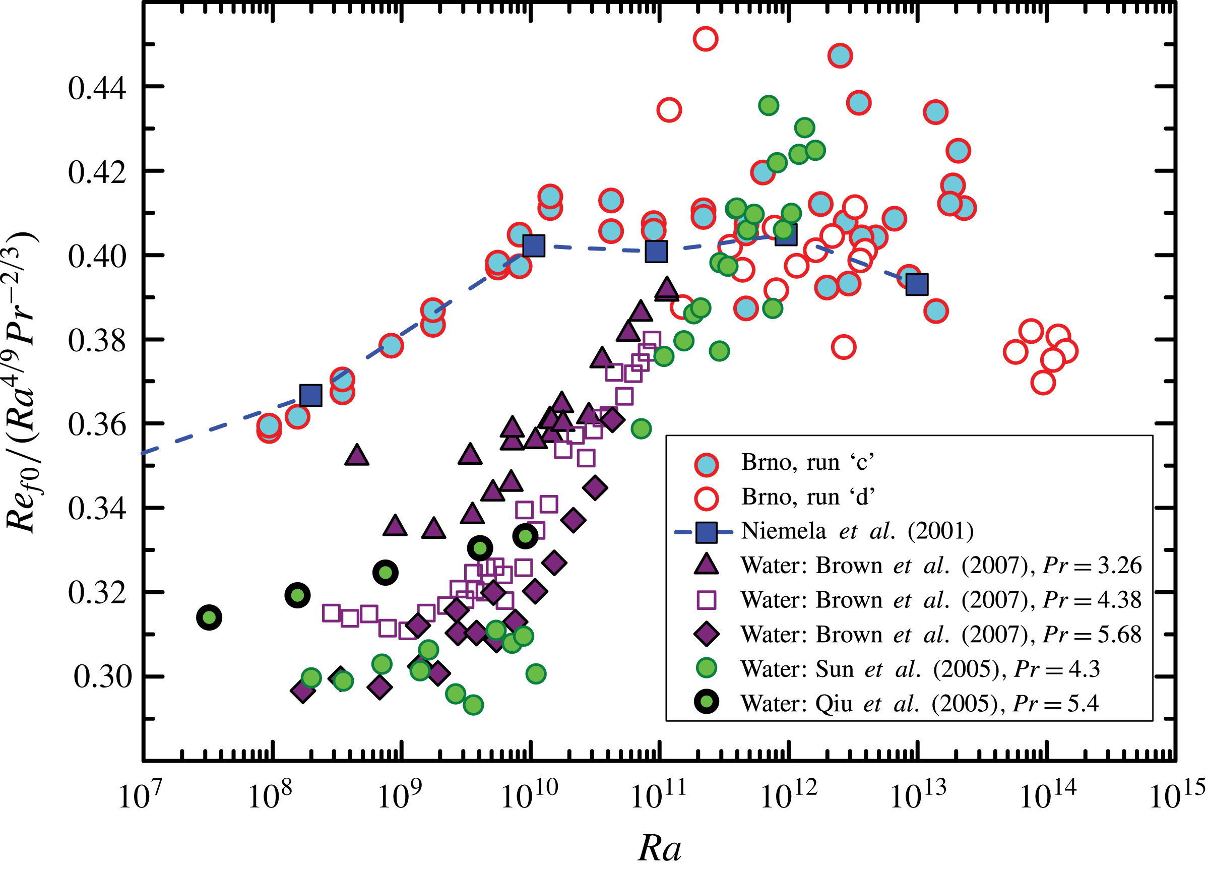
Frequency Reynolds number versus
 $\mathit{Ra}$
measured in cryogenic helium (Brno – our data, Niemela et al.
Reference Niemela, Skrbek, Sreenivasan and Donnelly2001) and water experiments at
 $3.3<\mathit{Pr}<5.7$
(Qiu & Tong Reference Qiu and Tong2001a
; Sun et al.
Reference Sun, Xia and Tong2005; Brown et al.
Reference Brown, Funfschilling and Ahlers2007) compensated by
 $\mathit{Ra}^{4/9}\mathit{Pr}^{-2/3}$
, as in figures 9 and 10.

Figure 11 shows for a comparison the data on the frequency Reynolds numbers
 $\mathit{Re}_{f0}$
from experiments with working fluids of higher Prandtl number values,
 $3.3<\mathit{Pr}<5.7$
(Qiu & Tong Reference Qiu and Tong2001a
; Sun et al.
Reference Sun, Xia and Tong2005; Brown et al.
Reference Brown, Funfschilling and Ahlers2007). Brown et al. (Reference Brown, Funfschilling and Ahlers2007) observed a sharp transition, from
 $\mathit{Re}_{f0}\propto \mathit{Ra}^{4/9}\mathit{Pr}^{-2/3}$
, to a regime with higher
 $\mathit{Ra}$
-scaling exponent; their findings are consistent with the results of water experiments conducted in the other laboratories. This result, obtained for higher
 $\mathit{Pr}$
sharply contrasts with the scaling observed at
 $\mathit{Pr}\simeq 0.7$
in cryogenic experiments, where, with increasing
 $\mathit{Ra}$
, a steeper scaling transits to the scaling
 $\mathit{Re}_{f0}\propto \mathit{Ra}^{4/9}\mathit{Pr}^{-2/3}$
. As well known, such a qualitatively different type of transition, as compared to the helium gas, is indeed captured by the GL theory (Grossmann & Lohse Reference Grossmann and Lohse2000, Reference Grossmann and Lohse2001, Reference Grossmann and Lohse2002, Reference Grossmann and Lohse2004) for the
 $\mathit{Pr}$
values corresponding to water. This transition, called
 $II_{u}{-}IV_{u}$
, is characterized by a cross-over from the boundary-layer-dominated to the bulk-dominated thermal dissipation. As discussed in Grossmann & Lohse (Reference Grossmann and Lohse2002), the theoretical
 $\mathit{Re}(\mathit{Ra})$
dependence (not shown here) displays a transition between a flatter dependence for
 $\mathit{Ra}$
below
 $10^{10}$
to a steeper one above
 $10^{10}$
(opposite to the helium case), qualitatively in line with the experimental dependence shown in figure 11. Nevertheless, the difference in the respective theoretical slopes above and below the transition is smaller than in the experimental data, in analogy to the situation in helium. For water, the discrepancy between the data and the GL description is even more severe, as the approximate scalings in the experiments are steeper on both sides of the transition than in the theory (with
 $\mathit{Re}\propto \mathit{Ra}^{4/9}$
seen above, not below
 $\mathit{Ra}\sim 10^{10}$
), calling again for a theoretical description incorporating more details of the LSC dynamics, or coherent structures in general.
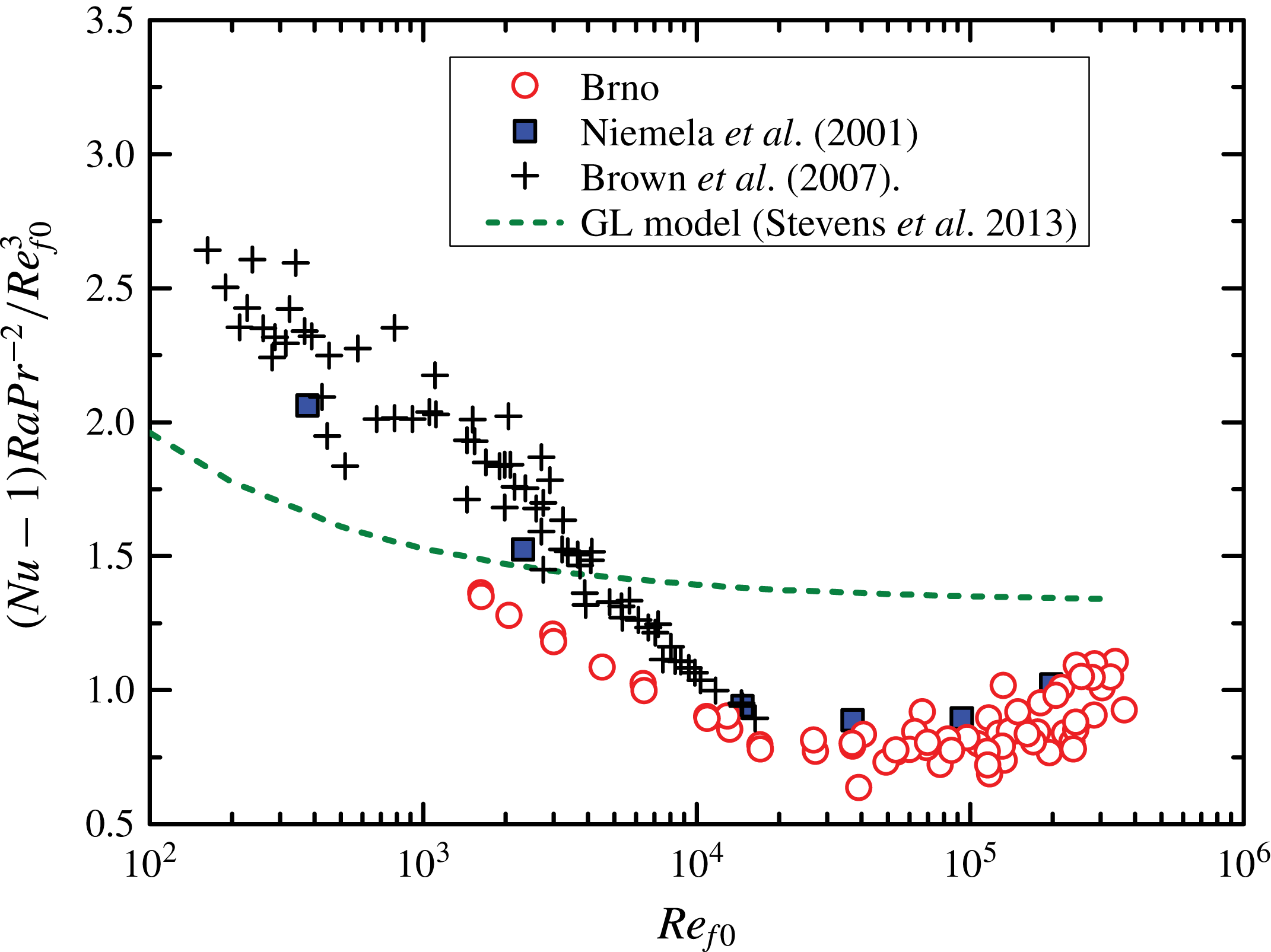
Comparison of
 $(Nu-1)Ra/Pr^{2}$
between our data and other experiments, plotted against the frequency Reynolds number
 $\mathit{Re}_{f0}$
. Solid blue squares correspond to the cryogenic helium data of Niemela et al. (Reference Niemela, Skrbek, Sreenivasan and Donnelly2001) and Niemela & Sreenivasan (Reference Niemela and Sreenivasan2003a
). Crosses are data from water experiment by Brown et al. (Reference Brown, Funfschilling and Ahlers2007). The dashed line represents the GL model fit by Stevens et al. (Reference Stevens, van der Poel, Grossmann and Lohse2013) for helium.

3.4 Scaling of kinetic energy dissipation
Finally, let us examine the relation between the exact formula of reduced mean energy dissipation rate,
 $e_{U}/(\unicode[STIX]{x1D708}^{3}L^{4})=(\mathit{Nu}-1)\mathit{Ra}/\mathit{Pr}^{2}$
, and calculated Reynolds numbers
 $\mathit{Re}_{f0}$
, as well as
 $\mathit{Re}_{p}$
and
 $\mathit{Re}_{U}$
,
 $\mathit{Re}_{V}$
,
 $\mathit{Re}_{eff}$
. To appreciate how closely our data agree with other investigators and with the Grossmann–Lohse theory in both the most recent version (Stevens et al.
Reference Stevens, van der Poel, Grossmann and Lohse2013), as well as the original version (Grossmann & Lohse Reference Grossmann and Lohse2001, Reference Grossmann and Lohse2002), figures 12 and 13 show the quantity
 $(\mathit{Nu}-1)\mathit{Ra}/\mathit{Pr}^{2}$
compensated by
 $\mathit{Re}_{f0}^{3}$
. First of all, we see that overall, the updated as well as the original GL do not describe the internally consistent cryogenic helium data at
 $\mathit{Re}_{f0}<20\,000$
(i.e. at
 $\mathit{Ra}<10^{10}$
), while for
 $\mathit{Re}>20\,000$
, the experimental and theoretical scaling exponents are consistent. This discrepancy was also observed by Brown et al. (Reference Brown, Funfschilling and Ahlers2007) in water experiments conducted for
 $\mathit{Ra}<10^{11}$
(see crosses in figure 12); they therefore attempted to solve this discrepancy by stating that
 $\mathit{Re}_{f0}$
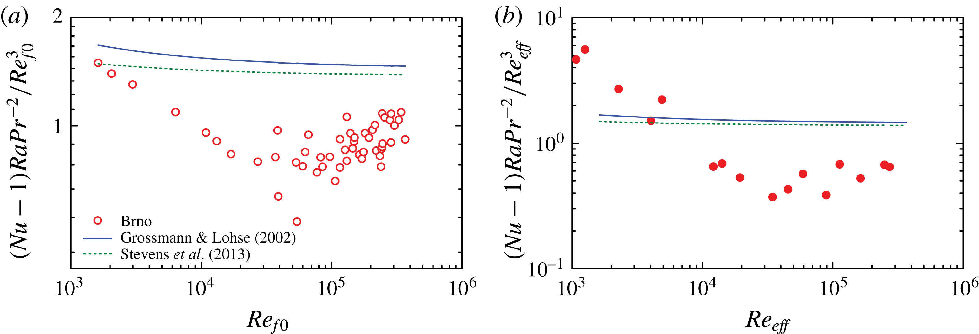
is not the appropriate Reynolds number. Indeed, it may appear more natural to relate the single Reynolds number of the GL model to the LCS circulation, rather than to the LSC sloshing. Thus we compare in figure 13 the GL predictions with our
 $(\mathit{Nu}-1)\mathit{Ra}/\mathit{Pr}^{2}$
data plotted against both
 $\mathit{Re}_{f0}$
(a) and
 $\mathit{Re}_{eff}$
(b). We see that the correspondence with the theory is in both cases problematic for the low
 $\mathit{Re}$
(and
 $\mathit{Ra}$
). To summarize, within the range
 $15\,000<(\mathit{Re}_{eff},\mathit{Re}_{f0})<20\,000$
, which corresponds to approximately
 $10^{10}$
in
 $\mathit{Ra}$
, a transition in scaling of the dissipation rate from an approximately
 $\mathit{Re}^{5/2}$
to approximately
 $\mathit{Re}^{3}$
(expected for domination of energy dissipation in the bulk), is observed in helium experiments, the latter being in qualitative agreement with the Grossmann–Lohse model. We note that the
 $\mathit{Nu}(\mathit{Ra})$
scaling, as discussed in Urban et al. (Reference Urban, Hanzelka, Králík, Musilová, Srnka and Skrbek2012), undergoes a change at somewhat higher
 $\mathit{Ra}$
, between
 $10^{10}$
and
 $10^{11}$
(where
 $\mathit{Pr}\approx 0.7$
,
 $\mathit{Re}_{f0}\approx 40\,000$
).
Values of reduced mean energy dissipation rate,
 $(Nu-1)Ra/Pr^{2}$
, in dependence on frequency-based Reynolds number
 $\mathit{Re}_{f0}$
(a) and the ‘elliptic’ number
 $\mathit{Re}_{eff}$
(b). The solid line represents the original fit of the Grossmann–Lohse model (Grossmann & Lohse Reference Grossmann and Lohse2001, Reference Grossmann and Lohse2002), while the dashed line is the updated fit by Stevens et al. (Reference Stevens, van der Poel, Grossmann and Lohse2013).

4 Summary and conclusions
We performed a statistical analysis of local temperature fluctuations in an aspect ratio one cryogenic helium RBC cell in a large range
 $10^{8}{-}10^{14}$
of Rayleigh numbers
 $\mathit{Ra}$
, aimed at determining the Reynolds numbers characterizing the large-scale circulation dynamics. From the temperature fluctuation PDFs and power spectra, we determined the mean wind/LSC orientation and its sloshing mode frequency. Further, we evaluated the signal auto-correlations
 $AC(\unicode[STIX]{x1D70F})$
at each individual sensor and the cross-correlations
 $CC(\unicode[STIX]{x1D70F},x)$
between the pairs of leading and trailing sensors on each side of the cell. From the former one-point measurements, we determined the sloshing mode frequency Reynolds number
 $\mathit{Re}_{f0}$
, while from the latter two-point measurements, we determined
 $\mathit{Re}_{p}$
(based on Taylor frozen flow hypothesis) and
 $\mathit{Re}_{U}$
,
 $Re_{V}$
,
 $Re_{eff}$
(based on the elliptic approximation of the space–time correlation function).
The first main result of this study is an experimental determination and discussion of these various Reynolds numbers: (i) we address the
 $\mathit{Re}(\mathit{Ra})$
dependencies, pointing out a transition in the dynamics of LSC at
 $\mathit{Ra}\approx 10^{10}{-}10^{11}$
, and (ii) we discuss their relation to the measurements of the Nusselt numbers, obtained within the same experiments (see Urban et al.
Reference Urban, Musilová and Skrbek2011, Reference Urban, Hanzelka, Králík, Musilová, Srnka and Skrbek2012, Reference Urban, Hanzelka, Musilová, Králík, La Mantia, Srnka and Skrbek2014). Further, we compare our data with other available high
 $\mathit{Ra}$
experiments. We find that both the one-point (
 $\mathit{Re}_{f0}$
) and two-point Reynolds numbers (
 $\mathit{Re}_{p}$
in particular), evaluated in the range
 $10^{8}<Ra<10^{14}$
, agree over this entire range with the
 $\unicode[STIX]{x1D6E4}=1$
results of the RBC experiment conducted by Niemela et al. (Reference Niemela, Skrbek, Sreenivasan and Donnelly2001). Moreover,
 $\mathit{Re}_{f0}$
roughly agrees also with the result of Castaing et al. (Reference Castaing, Gunaratne, Heslot, Kadanoff, Libchaber, Thomae, Wu, Zaleski and Zanetti1989) obtained in a smaller container (
 $\unicode[STIX]{x1D6E4}=1$
,
 $L=8.7~\text{cm}$
). For
 $\mathit{Re}_{p}$
, we also used the data from a
 $\unicode[STIX]{x1D6E4}=1/2$
experiment published by Chavanne et al. (Reference Chavanne, Chilla, Chabaud, Castaing and Hebral2001). Such a comparison is meaningful, considering the fact that the scaling of Nusselt number observed in numerous
 $\unicode[STIX]{x1D6E4}=1$
and
 $\unicode[STIX]{x1D6E4}=1/2$
experiments is similar (Stevens, Lohse & Verzicco Reference Stevens, Lohse and Verzicco2011). Close similarity of Reynolds number
 $\mathit{Re}_{p}$
scaling in our experiment and those of Chavanne et al. (Reference Chavanne, Chilla, Chabaud, Castaing and Hebral2001) and Niemela et al. (Reference Niemela, Skrbek, Sreenivasan and Donnelly2001) is found.
The second main result of this study is an observation of a transition between two types of scaling of LSC characteristics around
 $\mathit{Ra}\sim 10^{10}{-}10^{11}$
and
 $\mathit{Pr}\sim 0.7$
. Signatures of the transition are:
-
(i) scaling of Reynolds numbers varies from steeper to less steep
 $\mathit{Re}\propto \mathit{Ra}^{4/9}\mathit{Pr}^{-2/3}$
scaling;
-
(ii) mean energy dissipation rate
$(Nu-1)Ra/Pr^{2}$
changes sharply from
$\mathit{Re}^{5/2}$
to
$\mathit{Re}^{3}$
; -
(iii) skewness of temperature PDFs for the trailing sensors increases with
$\mathit{Ra}$
and saturates beyond
$\mathit{Ra}\approx 10^{10}$
, while for the leading sensors, this quantity is nearly constant throughout the entire studied range
$10^{8}{-}10^{14}$
of
$\mathit{Ra}$
.



In contrast, the PDF flatness
 $M_{4}$
data would require larger statistics to be conclusive about the transition.
The transition observed in the PDF skewness suggests a change in geometry of the LSC flow from an ellipse positioned diagonally across the cell to a more squarish shape, in line with the suggestion of Niemela & Sreenivasan (Reference Niemela and Sreenivasan2003b ) based on helium experiments and also with the direct PIV visualization in a water experiment by Sun et al. (Reference Sun, Xia and Tong2005).
From the theoretical perspective, let us note that a qualitatively similar change in
 $\mathit{Re}$
scaling (i.e. steeper-to-flatter dependence with increasing
 $\mathit{Ra}$
) at
 $\mathit{Ra}\sim 10^{10}{-}10^{11}$
follows from the GL model, if the original (Grossmann & Lohse Reference Grossmann and Lohse2001, Reference Grossmann and Lohse2002) parametrization is applied to our measured values of
 $\mathit{Pr}$
and
 $\mathit{Ra}$
. In particular, the change corresponds to the
 $IV_{l}{-}IV_{u}$
transition related to the cross-over between the thermal and viscous boundary layers. However, the experimental effect that we observe here is much more pronounced. Interestingly, an analogous situation can be noticed for the transition in water at
 $\mathit{Ra}\sim 10^{10}$
, where the experimental effect is again considerably more pronounced than the theory prediction. The GL theory predicts here a change from a flatter to a steeper Reynolds number scaling (notice that the ‘sense’ of the change is opposite to helium) associated with the
 $II_{u}{-}IV_{u}$
transition, related to cross-over from boundary-layer-dominated to bulk-dominated thermal energy dissipation.
The fact that the experimentally observed transition signatures are considerably more pronounced than in the established theory (see also Ahlers et al. Reference Ahlers, Grossmann and Lohse2009) in our opinion indicates that the LSC dynamics may considerably modify the effects at the interface of the bulk and the boundary layers. The situation calls for a refined theoretical model combining such LSC dynamics with a GL-like description and further dedicated experiments. We hope that the presented new experimental data and their analysis and comparison with other experiments can be regarded as a subsequent step to deeper understanding of thermally driven turbulent flows.
Acknowledgements
We thank many colleagues for stimulating discussions, especially S. Babuin, P. Hanzelka, X. He, M. Jackson, R. du Puits, P.-E. Roche, J. Salort, D. Schmoranzer and K. R. Sreenivasan. We acknowledge the support of this research by the Czech Science Foundation under the project GA17-03572S. M.M. acknowledges the support by the MEYS CR project LO1212.