1 Introduction
Understanding the dynamics of small particles in turbulent flows is relevant to a broad range of problems, such as aerosol manufacturing (Moody & Collins Reference Moody and Collins2003), drug delivery (Li et al.
Reference Li, Perzl, Heyder, Langer, Brain, Englemeier, Niven and Edwards1996), spray combustion (Faeth Reference Faeth1996), microorganism motion in aquatic environments (De Lillo et al.
Reference De Lillo, Cencini, Durham, Barry, Stocker, Climent and Boffetta2014) and planetesimal formation in the early universe (Johansen et al.
Reference Johansen, Oishi, Mac Low, Klahr and Henning2007). A great deal of research on the motion of particles at the small scales of turbulent flows has been motivated by the need to better understand the microphysical mechanisms governing atmospheric cloud formation, for which standard models can fail in important regimes (Shaw Reference Shaw2003; Grabowski & Wang Reference Grabowski and Wang2013). In particular, standard models of droplet growth in clouds capture two main mechanisms: (i) condensation, which is effective for droplets with radii smaller than
 $30~\unicode[STIX]{x03BC}\text{m}$
, and (ii) coalescence due to differential sedimentation, which is effective for drops with radii larger than
 $80~\unicode[STIX]{x03BC}\text{m}$
. In the intermediate size range of
 $30$
–
 $80~\unicode[STIX]{x03BC}\text{m}$
, neither mechanism can account for the rapid droplet growth observed in clouds, and hence this size range is commonly referred to as the ‘condensation-coalescence bottleneck’ or the ‘size gap’ (Pruppacher & Klett Reference Pruppacher and Klett1997). It is believed that turbulence-induced collisions lead to rapid growth in the size gap, although many open questions concerning this remain (Devenish et al.
Reference Devenish, Bartello, Brenguier, Collins, Grabowski, Ijzermans, Malinowski, Reeks, Vassilicos and Wang2012; Grabowski & Wang Reference Grabowski and Wang2013). Turbulence is understood to give rise to enhanced particle collision rates by generating spatial clustering of the particles, and by leading to enhanced collision velocities (Pumir & Wilkinson Reference Pumir and Wilkinson2016). Turbulence-induced collisions are also thought to be important for understanding the formation of protoplanetary disks, and the atmospheres of planets and dwarf stars (Cuzzi, Dobrovolskis & Hogan Reference Cuzzi, Dobrovolskis, Hogan, Hewins, Jones and Scott1996; Johansen et al.
Reference Johansen, Oishi, Mac Low, Klahr and Henning2007; Pan et al.
Reference Pan, Padoan, Scalo, Kritsuk and Norman2011).
In this paper we are concerned with the motion of small, heavy, inertial particles, namely, particles whose diameter is much smaller than the smallest length scale of the flow, and whose density is much greater than that of the fluid in which they are suspended. This regime is relevant in both the cloud and astrophysical contexts, and gas–solid flows in general. The small-scale motion of such particles in turbulence is controlled by a range of physical mechanisms, whose effect depends upon the particle Stokes number,
 $St\equiv \unicode[STIX]{x1D70F}_{p}/\unicode[STIX]{x1D70F}_{\unicode[STIX]{x1D702}}$
, where
 $\unicode[STIX]{x1D70F}_{p}$
is the particle response time,
 $\unicode[STIX]{x1D70F}_{\unicode[STIX]{x1D702}}$
is the Kolmogorov time scale. The inertia of such particles may be quantified by their Stokes number,
 $St\equiv \unicode[STIX]{x1D70F}_{p}/\unicode[STIX]{x1D70F}_{\unicode[STIX]{x1D702}}$
, where
 $\unicode[STIX]{x1D70F}_{p}$
is the particle response time,
 $\unicode[STIX]{x1D70F}_{\unicode[STIX]{x1D702}}\equiv (\unicode[STIX]{x1D708}/\unicode[STIX]{x1D716})^{1/2}$
is the Kolmogorov time scale,
 $\unicode[STIX]{x1D708}$
is the fluid kinematic viscosity and
 $\unicode[STIX]{x1D716}$
is the mean turbulent kinetic energy dissipation rate. In the cloud context, the relevant range of
 $St$
depends upon
 $\unicode[STIX]{x1D716}$
which can vary significantly. Siebert et al. (Reference Siebert, Gerashchenko, Gylfason, Lehmann, Collins, Shaw and Warhaft2010a
) show measurements from stratocumulus and small cumulus clouds that show
 $St\leqslant O(10^{-2})$
, while Siebert et al. (Reference Siebert, Shaw, Ditas, Schmeissner, Malinowski, Bodenschatz and Xu2015) reports
 $St\leqslant O(1)$
. Measurements reported by Vaillancourt & Yau (Reference Vaillancourt and Yau2000) and Jonas (Reference Jonas1996) show that
 $10^{-4}\lesssim \unicode[STIX]{x1D716}\lesssim 10^{-1}~\text{m}^{2}\text{s}^{-3}$
, which implies that droplets in the size gap have
 $0.01\lesssim St\lesssim 2$
(Ayala et al.
Reference Ayala, Rosa, Wang and Grabowski2008; Grabowski & Wang Reference Grabowski and Wang2013).
The motion of small, heavy particles in turbulence is controlled by a range of physical mechanisms, whose effect depends upon
 $St$
. One of the important effects is preferential sampling, which describes the fact that inertial particles tend to avoid regions of strong rotation due to the centrifuge effect, and favour strain dominated regions of the flow (Maxey Reference Maxey1987; Squires & Eaton Reference Squires and Eaton1991; Eaton & Fessler Reference Eaton and Fessler1994). In the regime
 $St\ll 1$
, preferential sampling is the sole mechanism by which inertia affects the particle motion, and it gives rise to spatial clustering of the particles (Chun et al.
Reference Chun, Koch, Rani, Ahluwalia and Collins2005). When
 $St\geqslant O(1)$
, the particles are strongly affected by the finite memory they possess of their interaction with the turbulence along their path history (Bragg & Collins Reference Bragg and Collins2014a
,Reference Bragg and Collins
b
). This path-history effect gives rise to ‘caustics’ (Wilkinson & Mehlig Reference Wilkinson and Mehlig2005), associated with inertial particles having very large relative velocities at small separations. The path-history effect also leads to strong spatial clustering of the particles through the non-local clustering mechanism (Bragg, Ireland & Collins Reference Bragg, Ireland and Collins2015a
,Reference Bragg, Ireland and Collins
b
). When
 $St\geqslant O(1)$
, the filtering effect is also important (Bec et al.
Reference Bec, Biferale, Boffetta, Celani, Cencini, Lanotte, Musacchio and Toschi2006; Ayyalasomayajula, Warhaft & Collins Reference Ayyalasomayajula, Warhaft and Collins2008), describing the lack of response of the inertial particles to flow fluctuations having time scales less than
 $\unicode[STIX]{x1D70F}_{p}$
.
These physical mechanisms have been primarily studied for the case of monodisperse particles; however, in almost all real systems, the particles are polydisperse. In clouds and many other problems, the particle collisions are usually binary due to the dilute particle loading (Grabowski & Wang Reference Grabowski and Wang2013), and furthermore, mixing and dispersion of the particles in the flow is typically analysed by considering the relative motion of particle pairs (Salazar & Collins Reference Salazar and Collins2009). In this case, the problem of polydispersity reduces to understanding the effect of bidispersity on the small-scale particle-pair motion. The polydisperse statistics can then be obtained through suitable integrals of the bidisperse statistics, weighted according to the size distribution of the particles. Several studies have considered how bidispersity affects the spatial clustering (Zhou, Wexler & Wang Reference Zhou, Wexler and Wang2001; Chun et al. Reference Chun, Koch, Rani, Ahluwalia and Collins2005; Pan et al. Reference Pan, Padoan, Scalo, Kritsuk and Norman2011; Chen & Jin Reference Chen and Jin2017), relative velocities (Pan, Padoan & Scalo Reference Pan, Padoan and Scalo2014a ,Reference Pan, Padoan and Scalo b ; Chen & Jin Reference Chen and Jin2017) and collisions (Zhou et al. Reference Zhou, Wexler and Wang2001; Pan & Padoan Reference Pan and Padoan2014) of particles in turbulence. It was found that bidispersity reduces the clustering of inertial particles in turbulent flows (Zhou et al. Reference Zhou, Wexler and Wang2001; Chun et al. Reference Chun, Koch, Rani, Ahluwalia and Collins2005; Pan et al. Reference Pan, Padoan, Scalo, Kritsuk and Norman2011; Chen & Jin Reference Chen and Jin2017), whereas it enhances their relative velocities (Kruis & Kusters Reference Kruis and Kusters1997; Zhou et al. Reference Zhou, Wexler and Wang2001; Chen & Jin Reference Chen and Jin2017). Bidispersity was found to increase collision rates, since the enhancement of the collision velocities due to bidispersity outweighs the reduction in the clustering (Pan & Padoan Reference Pan and Padoan2014). We defer discussion of the physical mechanisms responsible for these effects of bidispersity to § 2.
In the context of cloud microphysics and many other applications, another effect that is crucial to account for is the effect of gravity on the particle motion. The relative importance of gravity to the turbulent accelerations can be quantified by the Froude number
 $Fr\equiv \unicode[STIX]{x1D716}^{3/4}/(\unicode[STIX]{x1D708}^{1/4}\mathfrak{g})$
, where
 $\unicode[STIX]{x1D716}$
is the mean fluid kinetic energy dissipation rate,
 $\unicode[STIX]{x1D708}$
is the kinematic viscosity (such that
 $\unicode[STIX]{x1D716}^{3/4}/\unicode[STIX]{x1D708}^{1/4}$
is the Kolmogorov acceleration scale) and
 $\mathfrak{g}$
is the magnitude of the gravitational acceleration vector. In atmospheric clouds, the relevant range of
 $Fr$
is mainly determined by
 $\unicode[STIX]{x1D716}$
, which, as noted earlier, varies significantly in clouds. Measurements in the atmosphere indicate
 $0.05\leqslant Fr\leqslant 0.3$
(Siebert, Shaw & Warhaft Reference Siebert, Shaw and Warhaft2010b
; Ireland, Bragg & Collins Reference Ireland, Bragg and Collins2016b
).
The impact of varying
 $Fr$
has recently been investigated for the case of monodisperse particles (Bec, Homann & Ray Reference Bec, Homann and Ray2014; Gustavsson, Vajedi & Mehlig Reference Gustavsson, Vajedi and Mehlig2014; Ireland et al.
Reference Ireland, Bragg and Collins2016b
). These studies found that reducing
 $Fr$
always reduces the relative velocities of the inertial particles, but has a non-trivial effect on the clustering, such that in some regimes of
 $St$
and
 $Fr$
, gravity reduces clustering and in other regimes it enhances clustering. Parishani et al. (Reference Parishani, Ayala, Rosa, Wang and Grabowski2015) and Ireland et al. (Reference Ireland, Bragg and Collins2016b
) also showed that gravity can significantly enhance inertial particle accelerations, although the explanations they gave for this behaviour were very different (see § 2).
Despite being crucial for understanding droplet motion in clouds and many other problems, it appears that the effect of gravity on the small-scale dynamics of bidisperse particles in turbulence has scarcely been addressed. Indeed, to the best of our knowledge, the only studies that have attempted to address this are those by Woittiez, Jonker & Portela (Reference Woittiez, Jonker and Portela2009) and Parishani et al. (Reference Parishani, Ayala, Rosa, Wang and Grabowski2015). The direct numerical simulations (DNS) study of Woittiez et al. (Reference Woittiez, Jonker and Portela2009) showed that gravity leads to a strong suppression of the clustering of bidisperse particles, but a strong enhancement of their collision velocities, due to the contribution from the differential settling of the particles. Furthermore, they found that the collision kernel based on bidisperse particles settling in quiescent flow significantly underpredicted the collision rates measured in their DNS. However, their study did not comprehensively explore the effects of varying the bidispersity and
 $Fr$
, and also focused exclusively on particle collisions, rather than more general small-scale processes. The DNS study of Parishani et al. (Reference Parishani, Ayala, Rosa, Wang and Grabowski2015) presented a preliminary study on the influence of gravity and bidispersity on the relative velocities of particle pairs in turbulence. Their approach was to decompose the relative velocity of the particle pair into various contributions that emerge from the particle equation of motion, and then analyse some of the statistics of those contributions. While interesting, these results do not give clear insight into how gravity and bidispersity affect particle-pair dynamics in turbulence, since the statistics of the relative velocities depend not only on the individual behaviour of these contributions, but also on various correlations between these contributions, and this was not examined in Parishani et al. (Reference Parishani, Ayala, Rosa, Wang and Grabowski2015). Also, they only considered the relative velocities at the contact separation, and therefore how gravity and bidispersity affects the relative motion of the particle pair at different scales/separations is unknown. There therefore remain many open questions with respect to how gravity affects bidisperse particle motion at the small scales of turbulence, and these knowledge gaps motivate the present work.
The organization of the paper is as follows. In § 2, we consider theoretically the effect of bidispersity and gravity on the relative motion of particle pairs at the small scales of turbulence. In § 3, we explain the numerical methods and parameters for our simulations. In § 4, we present the results of our simulations, exploring how bidispersity and
 $Fr$
impact the particle relative velocities, clustering and collisions. Finally, in § 5, we draw conclusions and highlight open issues that remain to be explored.
2 Theoretical considerations
For investigating the motion of droplets in clouds, it is usually assumed (e.g. Shaw Reference Shaw2003; Grabowski & Wang Reference Grabowski and Wang2013) that the particle loading is sufficiently small to ignore the effect of the particles on the turbulence (i.e. the system is ‘one-way coupled’), and that the particles are well described as being small (i.e.
 $d/\unicode[STIX]{x1D702}\ll 1$
, where
 $d$
is the particle diameter and
 $\unicode[STIX]{x1D702}$
is the Kolmogorov length scale) and heavy (
 $\unicode[STIX]{x1D70C}_{p}/\unicode[STIX]{x1D70C}\gg 1$
, where
 $\unicode[STIX]{x1D70C}_{p}$
is the particle density and
 $\unicode[STIX]{x1D70C}$
is the fluid density). Under these conditions, each particle is treated as a point particle whose motion obeys a simplified version of the equation by Maxey & Riley (Reference Maxey and Riley1983),
 $$\begin{eqnarray}\displaystyle & \displaystyle \dot{\boldsymbol{x}}^{p}(t)=\boldsymbol{v}^{p}(t), & \displaystyle\end{eqnarray}$$
 $$\begin{eqnarray}\displaystyle & \displaystyle \ddot{\boldsymbol{x}}^{p}(t)=\dot{\boldsymbol{v}}^{p}(t)=\frac{\boldsymbol{u}(\boldsymbol{x}^{p}(t),t)-\boldsymbol{v}^{p}(t)}{\unicode[STIX]{x1D70F}_{p}}+\mathfrak{g}, & \displaystyle\end{eqnarray}$$
where
 $\boldsymbol{x}^{p}(t)$
and
 $\boldsymbol{v}^{p}(t)$
are the particle position and velocity, respectively,
 $\unicode[STIX]{x1D70F}_{p}=\unicode[STIX]{x1D70C}_{p}d^{2}/18\unicode[STIX]{x1D707}$
is the particle response time (
 $\unicode[STIX]{x1D707}$
is the fluid dynamic viscosity) and
 $\boldsymbol{\mathfrak{g}}$
is the gravitational acceleration. As discussed in Ireland et al. (Reference Ireland, Bragg and Collins2016b
), the use of a linear rather than nonlinear drag force for the particles is likely sufficient for
 $St\leqslant O(1)$
, which is the range we restrict attention to in this study. Furthermore, using a linear drag force facilitates comparison with previous studies on the effect of gravity on the small-scale motion of monodisperse particles in turbulence that were also based on a linear drag force (Bec et al.
Reference Bec, Homann and Ray2014; Gustavsson et al.
Reference Gustavsson, Vajedi and Mehlig2014; Ireland et al.
Reference Ireland, Bragg and Collins2016b
).
We are interested in understanding how settling, bidisperse particle pairs move relative to each other, especially at the small scales of turbulence. We therefore consider the motion of a ‘satellite’ particle relative to a ‘primary’ particle, for which the equation of relative motion is obtained by subtracting (2.2) for the primary particle from that for the satellite particle,
 $$\begin{eqnarray}\ddot{\boldsymbol{r}}\hspace{0.5pt}^{p}(t)=\dot{\boldsymbol{w}}^{p}(t)=\frac{\unicode[STIX]{x0394}\boldsymbol{u}(\boldsymbol{x}^{p}(t),\boldsymbol{r}\hspace{0.5pt}^{p}(t),t)-\boldsymbol{w}^{p}(t)}{\unicode[STIX]{x1D70F}_{p}}+\frac{\unicode[STIX]{x1D703}\left(\boldsymbol{a}^{p}(t)-\mathfrak{g}\right)}{\unicode[STIX]{x1D70F}_{p}},\end{eqnarray}$$
where
 $\boldsymbol{x}^{p}(t)$
and
 $\boldsymbol{x}^{p}(t)+\boldsymbol{r}^{p}(t)$
are the positions of the primary and satellite particles, respectively,
 $\boldsymbol{w}^{p}(t)$
is their relative velocity,
 $$\begin{eqnarray}\displaystyle & \displaystyle \unicode[STIX]{x0394}\boldsymbol{u}(\boldsymbol{x}^{p}(t),\boldsymbol{r}\hspace{0.5pt}^{p}(t),t)\equiv \boldsymbol{u}(\boldsymbol{x}^{p}(t)+\boldsymbol{r}\hspace{0.5pt}^{p}(t),t)-\boldsymbol{u}(\boldsymbol{x}^{p}(t),t) & \displaystyle\end{eqnarray}$$
is the difference in the fluid velocity at the two particle positions,
 $\unicode[STIX]{x1D70F}_{p}$
is now the response time of the satellite particle,
 $\unicode[STIX]{x1D703}\equiv \unicode[STIX]{x0394}\unicode[STIX]{x1D70F}_{p}$
is the response time of the satellite particle subtracted from that of the primary particle, and
 $\boldsymbol{a}^{p}(t)=(\unicode[STIX]{x1D703}+\unicode[STIX]{x1D70F}_{p})^{-1}(\boldsymbol{u}(\boldsymbol{x}^{p}(t),t)-\boldsymbol{v}^{p}(t))+\boldsymbol{\mathfrak{g}}$
is the primary particle acceleration. Since we are considering homogeneous turbulence, we will drop the
 $\boldsymbol{x}^{p}(t)$
argument from statistical quantities.
If we non-dimensionalize the variables in (2.3) using appropriate combinations of the Kolmogorov acceleration
 $a_{\unicode[STIX]{x1D702}}$
, velocity
 $u_{\unicode[STIX]{x1D702}}$
, length
 $\unicode[STIX]{x1D702}$
and time
 $\unicode[STIX]{x1D70F}_{\unicode[STIX]{x1D702}}$
scales, we obtain
 $$\begin{eqnarray}\widetilde{\ddot{\boldsymbol{r}}\hspace{0.5pt}^{p}}(\tilde{t})=\widetilde{\dot{\boldsymbol{w}}^{p}}(\tilde{t})=\frac{\unicode[STIX]{x0394}\widetilde{\boldsymbol{u}}(\widetilde{\boldsymbol{x}^{p}}(\tilde{t}),\widetilde{\boldsymbol{r}\hspace{0.5pt}^{p}}(\tilde{t}),\tilde{t})-\widetilde{\boldsymbol{w}^{p}}(\tilde{t})}{St_{2}}+\frac{\unicode[STIX]{x0394}St\left(\widetilde{\boldsymbol{a}^{p}}(\tilde{t})-\boldsymbol{e}_{\mathfrak{g}}Fr^{-1}\right)}{St_{2}},\end{eqnarray}$$
where
 $\widetilde{\cdot }$
denotes a non-dimensional quantity,
 $St_{2}\equiv \unicode[STIX]{x1D70F}_{p}/\unicode[STIX]{x1D70F}_{\unicode[STIX]{x1D702}}$
is the Stokes number of the satellite particle,
 $\unicode[STIX]{x0394}St\equiv \unicode[STIX]{x1D703}/\unicode[STIX]{x1D70F}_{\unicode[STIX]{x1D702}}\equiv St_{1}-St_{2}$
, where
 $St_{1}$
is the Stokes number of the primary particle, and
 $\boldsymbol{e}_{\mathfrak{g}}$
is the unit vector in the direction of gravity. Another important parameter that we shall make use of is the scale-dependent Stokes number
 $St_{r}\equiv \unicode[STIX]{x1D70F}_{p}/\unicode[STIX]{x1D70F}_{r}$
, where
 $\unicode[STIX]{x1D70F}_{r}$
is the eddy turnover time at scale
 $r$
.
2.1 Relative velocities and particle accelerations
To gain insight into the effect of bidispersity and gravity on the particle-pair relative velocities, it is informative to consider the formal solution of (2.5), namely (in the rest of this section we drop
 $\widetilde{\cdot }$
for notational ease)
 $$\begin{eqnarray}\boldsymbol{w}^{p}(t)=\frac{1}{St_{2}}\int _{0}^{t}\text{e}^{-(t-s)/St_{2}}\unicode[STIX]{x0394}\boldsymbol{u}^{p}(s)\,\text{d}s-\unicode[STIX]{x0394}StFr^{-1}\boldsymbol{e}_{\mathfrak{ g}}+\frac{\unicode[STIX]{x0394}St}{St_{2}}\int _{0}^{t}\text{e}^{-(t-s)/St_{2}}\boldsymbol{a}^{p}(s)\,\text{d}s,\end{eqnarray}$$
where
 $\unicode[STIX]{x0394}\boldsymbol{u}^{p}(s)\equiv \unicode[STIX]{x0394}\boldsymbol{u}(\boldsymbol{x}^{p}(s),\boldsymbol{r}^{p}(s),s)$
. In (2.6), and throughout, we assume
 $t\gg St_{2}$
such that initial conditions/effects can be ignored (valid since we are interested in the statistically stationary state of the system).
In the monodisperse case,
 $\unicode[STIX]{x0394}St=0$
, and only the first integral in (2.6) remains. This case has been studied in great detail using theoretical and numerical approaches (Bec et al.
Reference Bec, Biferale, Cencini, Lanotte and Toschi2010; Gustavsson & Mehlig Reference Gustavsson and Mehlig2011; Salazar & Collins Reference Salazar and Collins2012b
; Bragg & Collins Reference Bragg and Collins2014b
; Gustavsson et al.
Reference Gustavsson, Vajedi and Mehlig2014; Ireland, Bragg & Collins Reference Ireland, Bragg and Collins2016a
; Ireland et al.
Reference Ireland, Bragg and Collins2016b
). Here we summarize the findings and refer the reader to those papers for detailed discussions.
When
 $St_{r}$
is finite, the inertial particles preferentially sample the fluid velocity field, showing a tendency to avoid regions of strong rotation due to the centrifuge effect, and accumulate in regions of strain (Maxey Reference Maxey1987). At scales outside of the dissipation range, the same effect occurs and can be understood in terms of the particle interaction with the coarse-grained strain and rotation fields at those scales (Bragg et al.
Reference Bragg, Ireland and Collins2015a
). When
 $St_{r}\geqslant O(1)$
, the dynamics becomes temporally non-local;
 $\boldsymbol{w}^{p}(t)$
depends upon
 $\unicode[STIX]{x0394}\boldsymbol{u}^{p}$
along the path history of the particle pair over the time span
 $t-s\leqslant O(\unicode[STIX]{x1D70F}_{p})$
. In the dissipation and inertial ranges where the statistics of
 $\unicode[STIX]{x0394}\boldsymbol{u}$
depend upon separation, this can have a dramatic effect. In particular, if the particle separation changes substantially over a time span
 $O(\unicode[STIX]{x1D70F}_{p})$
, then the particle pairs will remember their interaction with scales of motion of the turbulence that have very different properties from those at their current separation. This ‘path-history effect’ gives rise to ‘caustics’ (Wilkinson & Mehlig Reference Wilkinson and Mehlig2005), where
 $\Vert \boldsymbol{w}^{p}(t)\Vert \gg \Vert \unicode[STIX]{x0394}\boldsymbol{u}^{p}(t)\Vert$
at small separations. Finally, when
 $St_{r}\geqslant O(1)$
there also exists the ‘filtering effect’, which describes the fact that due to their inertia, the particles cannot fully respond to all of the turbulent fluctuations and so behave sluggishly.
In the dissipation range, the path-history effect dominates the behaviour of
 $\boldsymbol{w}^{p}(t)$
when
 $St_{r}\geqslant O(1)$
. As the separation increases, the path-history effect remains important when
 $St_{r}\geqslant O(1)$
, but its effect weakens because the separation dependence of
 $\unicode[STIX]{x0394}\boldsymbol{u}$
weakens. In this case, the preferential sampling and filtering effects play important roles. Finally, at the large scales of homogeneous turbulence, the path-history effect vanishes (since the statistics of
 $\unicode[STIX]{x0394}\boldsymbol{u}$
no longer depend upon separation), the preferential sampling plays a weak role, and the filtering effect dominates.
When
 $\unicode[STIX]{x0394}St=0$
, the effect of gravity on
 $\boldsymbol{w}^{p}(t)$
is only implicit; gravity affects
 $\unicode[STIX]{x0394}\boldsymbol{u}^{p}$
by changing the way the particles interact with the turbulent flow, and most importantly, by reducing the correlation time scale of
 $\unicode[STIX]{x0394}\boldsymbol{u}^{p}$
. This leads to a reduction of the preferential sampling and path-history effects (and therefore a reduction of caustics), and to an enhancement of the filtering effect (see Ireland et al. (Reference Ireland, Bragg and Collins2016b
) for a detailed discussion of these effects).
When
 $|\unicode[STIX]{x0394}St|>0$
and
 $Fr=\infty$
(i.e. no gravity), the main effect of the bidispersity is through the ‘acceleration term’ in (2.6), with an implicit effect upon the first integral in (2.6) through the modification to the properties of
 $\unicode[STIX]{x0394}\boldsymbol{u}^{p}$
. An essential difference between the two integrals in (2.6) is that the first depends upon the particle separation, whereas the second does not. Since
 $\unicode[STIX]{x0394}\boldsymbol{u}^{p}$
decreases, on average, with decreasing separation, then provided
 $|\unicode[STIX]{x0394}St|>0$
, there will be a separation below which the second integral is
 $\gg$
than the first. In this regime, the statistics of
 $\boldsymbol{w}^{p}(t)$
will not depend upon the particle separation. This acceleration contribution causes the relative velocities of bidisperse particles to exceed those of monodisperse particles at small separations, as observed in a number of previous theoretical and numerical studies (Zhou et al.
Reference Zhou, Wexler and Wang2001; Zaichik, Simonin & Alipchenkov Reference Zaichik, Simonin and Alipchenkov2006; Zaichik et al.
Reference Zaichik, Fede, Simonin and Alipchenkov2009; Pan & Padoan Reference Pan and Padoan2010; Pan et al.
Reference Pan, Padoan and Scalo2014b
). In homogeneous turbulence, there is no path-history effect associated with the second integral in (2.6); the statistical properties of
 $\boldsymbol{a}^{p}(s)$
are equivalent along all primary particle trajectories
 $\boldsymbol{x}^{p}$
. The accelerations are, however, strongly affected by both the preferential sampling and filtering effects (Bec et al.
Reference Bec, Biferale, Boffetta, Celani, Cencini, Lanotte, Musacchio and Toschi2006; Ayyalasomayajula et al.
Reference Ayyalasomayajula, Warhaft and Collins2008; Salazar & Collins Reference Salazar and Collins2012a
; Ireland et al.
Reference Ireland, Bragg and Collins2016b
), with filtering causing the fluctuations of
 $\boldsymbol{a}^{p}$
to decrease rapidly with increasing
 $St$
.
When
 $|\unicode[STIX]{x0394}St|>0$
and
 $Fr<\infty$
, gravity can lead to a number of effects on the relative motion of bidisperse particles. First, we note that the role of gravity in (2.5) is a little subtle since
 $\boldsymbol{a}^{p}(t)-\boldsymbol{e}_{\mathfrak{g}}Fr^{-1}=St_{1}^{-1}(\boldsymbol{u}(\boldsymbol{x}^{p}(t),t)-\boldsymbol{v}^{p}(t))$
, i.e. the explicit role of gravity appears to be absent. However, the direct effect of gravity is hidden in
 $\boldsymbol{v}^{p}(t)$
, which may be brought out using the formal solution for
 $\boldsymbol{v}^{p}(t)$
to obtain
 $$\begin{eqnarray}\displaystyle \boldsymbol{a}^{p}(t) & = & \displaystyle \displaystyle \frac{1}{St_{1}}\left(\boldsymbol{u}(\boldsymbol{x}^{p}(t),t)-\boldsymbol{v}^{p}(t)\right)+\boldsymbol{e}_{\mathfrak{g}}Fr^{-1}\nonumber\\ \displaystyle & = & \displaystyle \displaystyle \frac{1}{St_{1}}\left(\boldsymbol{u}(\boldsymbol{x}^{p}(t),t)-\frac{1}{St_{1}}\int _{0}^{t}\text{e}^{-(t-t^{\prime })/St_{1}}\boldsymbol{u}^{p}(t^{\prime })\,\text{d}t^{\prime }-St_{1}\left[1-\text{e}^{-t/St_{1}}\right]\boldsymbol{e}_{\mathfrak{g}}Fr^{-1}\right)+\boldsymbol{e}_{\mathfrak{g}}Fr^{-1}\nonumber\\ \displaystyle & = & \displaystyle \displaystyle \frac{1}{St_{1}^{2}}\int _{0}^{t}\text{e}^{-(t-t^{\prime })/St_{1}}\left(\boldsymbol{u}^{p}(t)-\boldsymbol{u}^{p}(t^{\prime })\right)\,\text{d}t^{\prime },\end{eqnarray}$$
where we have again assumed
 $t\gg St_{1}$
. The important point then is that
 $\boldsymbol{a}^{p}$
is in fact only implicitly affected by gravity, despite the fact that gravity appears explicitly in its dynamical equation.
The effect of gravity on the first term on the right-hand side of (2.6) is qualitatively the same as in the monodisperse case, described earlier. The effect of gravity on the second term on the right-hand side of (2.6) is clear; it increases as
 $Fr$
decreases, and becomes increasingly important as
 $|\unicode[STIX]{x0394}St|$
increases. However, this term only acts in the direction of gravity, and plays no role in the plane normal to this. Therefore, in the plane normal to
 $\boldsymbol{e}_{\mathfrak{g}}$
the effect of gravity is only implicit. The third term on the right-hand side of (2.6) involves
 $\boldsymbol{a}^{p}$
, and in Ireland et al. (Reference Ireland, Bragg and Collins2016b
) we showed that gravity can enhance
 $\boldsymbol{a}^{p}$
, the effect being dramatic when
 $Fr\ll 1$
. This enhancement of inertial particle accelerations due to gravity was also observed by Parishani et al. (Reference Parishani, Ayala, Rosa, Wang and Grabowski2015), who proposed that the enhancement is due to the preferential sweeping effect (Wang & Maxey Reference Wang and Maxey1993). However, in Ireland et al. (Reference Ireland, Bragg and Collins2016b
) we argued that this cannot be the explanation since the acceleration enhancement due to gravity is strongest in a regime of
 $St$
and
 $Fr$
where the preferential sampling of the fluid velocity gradient field is absent. We argued, in contrast, that the acceleration enhancement occurs because when
 $St$
is finite, the inertial particles have large settling velocities when
 $Fr$
is small, causing the fluid velocity seen by the particles to change rapidly in time. That is, fast settling leads to large values of
 $\boldsymbol{u}^{p}(t)-\boldsymbol{u}^{p}(t^{\prime })$
even when
 $t-t^{\prime }\ll St$
, which in turn through (2.7) implies large fluctuations in
 $\boldsymbol{a}^{p}(t)$
. Further, we showed in Ireland et al. (Reference Ireland, Bragg and Collins2016b
) that fluctuations in
 $\boldsymbol{a}^{p}(t)$
are weaker in the direction of gravity than in the plane normal to gravity, which we explained in terms of the difference in the longitudinal and transverse correlation length scales of
 $\boldsymbol{u}$
in isotropic turbulence.
In the plane normal to gravity, the third term, which always dominates over the first term at sufficiently small separations, can increase as
 $Fr$
is decreased due to the enhanced accelerations. In Ireland et al. (Reference Ireland, Bragg and Collins2016b
) we derived a theoretical model for the effect of strong gravity on the particle accelerations. For simplicity, let us define the gravitational force to act in the
 $x_{3}$
direction, so that
 $\boldsymbol{e}_{\mathfrak{g}}=(0,0,1)$
. This will be referred to as the ‘vertical’ direction, whereas
 $x_{1}$
and
 $x_{2}$
will be referred to as the ‘horizontal’ directions. (Note also that since we are considering isotropic turbulence, the statistics of the particle motion are axisymmetric about
 $\boldsymbol{e}_{\mathfrak{g}}$
when
 $Fr<\infty$
.) Using this notation, the result derived in Ireland et al. (Reference Ireland, Bragg and Collins2016b
) for the inertial particle accelerations in the horizontal direction is
 $$\begin{eqnarray}\displaystyle \frac{\langle a_{1}^{p}(t)a_{1}^{p}(t)\rangle }{a_{\unicode[STIX]{x1D702}}^{2}}=Fr^{-1}\left(\frac{u^{\prime }}{u_{\unicode[STIX]{x1D702}}}\right)^{2}\left(\frac{1}{St_{1}^{2}Fr^{-1}+\ell \unicode[STIX]{x1D702}^{-1}}\right),\quad \text{for}\,\,St_{1}Fr^{-1}\gg u^{\prime }u_{\unicode[STIX]{x1D702}}^{-1}, & & \displaystyle\end{eqnarray}$$
where
 $u^{\prime }$
is the fluid root-mean-square (r.m.s.) velocity, and
 $\ell$
is the integral length scale of the flow. Comparisons of (2.8) with DNS in Ireland et al. (Reference Ireland, Bragg and Collins2016b
) showed excellent agreement in the regime
 $St_{1}Fr^{-1}\gg u^{\prime }u_{\unicode[STIX]{x1D702}}^{-1}$
. For fixed
 $R_{\unicode[STIX]{x1D706}}$
, (2.8) increases as
 $Fr$
decreases, resulting in strong accelerations in the plane normal to gravity. Since
 $w_{1}^{p}$
depends upon
 $a_{1}^{p}$
, gravity can therefore lead to an enhancement of the relative velocities in the plane normal to its action, and this enhancement could be strong when
 $Fr\ll 1$
.
Finally, consider the limit
 $Fr\rightarrow 0$
where the relative velocities in the vertical direction are deterministic and given by
 $$\begin{eqnarray}w_{3}^{p}(t)=-\unicode[STIX]{x0394}StFr^{-1},\end{eqnarray}$$
which is simply the difference in the Stokes settling velocities of the two particles (i.e. the differential settling velocity), in dimensionless form. However, in the horizontal directions, if
 $R_{\unicode[STIX]{x1D706}}\gg 1$
the motion remains turbulent even in the limit
 $Fr\rightarrow 0$
since
 $$\begin{eqnarray}w_{1}^{p}(t)=\frac{1}{St_{2}}\int _{0}^{t}\text{e}^{-(t-s)/St_{2}}\unicode[STIX]{x0394}u_{1}^{p}(s)\,\text{d}s+\frac{\unicode[STIX]{x0394}St}{St_{2}}\int _{0}^{t}\text{e}^{-(t-s)/St_{2}}a_{1}^{p}(s)\,\text{d}s.\end{eqnarray}$$
The effect of gravity is implicit in (2.10), and in the limit
 $Fr\rightarrow 0$
the large settling velocities of the particles causes them to experience
 $\unicode[STIX]{x0394}u_{1}^{p}$
as a white noise signal (Bec et al.
Reference Bec, Homann and Ray2014). As such, the limit
 $Fr\rightarrow 0$
is subtle in the bidisperse case. In the vertical direction,
 $w_{3}^{p}(t)=-\unicode[STIX]{x0394}StFr^{-1}$
when
 $Fr\rightarrow 0$
, which applies to quiescent and turbulent flows. However, for the horizontal direction, in a quiescent flow
 $w_{1}^{p}(t)=0\,\forall Fr$
, but in a turbulent flow,
 $w_{1}^{p}(t)\neq 0$
in the limit
 $Fr\rightarrow 0$
. As a consequence of this,
 $\lim _{Fr\rightarrow 0}\boldsymbol{w}^{p}(t)\not \rightarrow -\unicode[STIX]{x0394}StFr^{-1}\boldsymbol{e}_{\mathfrak{g}}$
in a turbulent flow.
Furthermore, provided
 $R_{\unicode[STIX]{x1D706}}<\infty$
, then in the limit
 $Fr\rightarrow 0$
(2.8) becomes
 $$\begin{eqnarray}\displaystyle & \displaystyle \frac{\langle a_{1}^{p}(t)a_{1}^{p}(t)\rangle }{a_{\unicode[STIX]{x1D702}}^{2}}=\left(\frac{u^{\prime }}{St_{1}u_{\unicode[STIX]{x1D702}}}\right)^{2}\sim \frac{R_{\unicode[STIX]{x1D706}}}{St_{1}^{2}}, & \displaystyle\end{eqnarray}$$
which is independent of
 $Fr$
. This predicts that even in the limit
 $Fr\rightarrow 0$
, turbulence can lead to horizontal accelerations for the inertial particles that are not only finite, but
 $\gg a_{\unicode[STIX]{x1D702}}$
.
In Chang, Malec & Shaw (Reference Chang, Malec and Shaw2015) a semi-empirical formula for the second-order structure function
 $\langle \Vert \boldsymbol{w}^{p}(t)\Vert ^{2}\rangle _{\boldsymbol{r}}$
was constructed for
 $St_{2}\ll 1$
and
 $|\unicode[STIX]{x0394}St|\ll 1$
, where
 $\langle \cdot \rangle _{\boldsymbol{r}}$
denotes an ensemble average conditioned on
 $\boldsymbol{r}^{p}(t)=\boldsymbol{r}$
. By comparing their results with DNS data for
 $Fr=0.1$
, they found good agreement between their prediction and the DNS data even when
 $St_{2}=O(1)$
(with
 $|\unicode[STIX]{x0394}St|\ll 1$
). However, this is mainly because in their data with
 $Fr=0.1$
,
 $\langle \Vert \boldsymbol{w}^{p}(t)\Vert ^{2}\rangle _{\boldsymbol{r}}\approx (\unicode[STIX]{x0394}St)^{2}Fr^{-2}$
for small
 $r/\unicode[STIX]{x1D702}$
, i.e. the turbulent contribution is negligible, and this gravitational settling contribution is in exact, closed form for arbitrary
 $St_{2}$
,
 $\unicode[STIX]{x0394}St$
. Deriving closed form predictions for
 $\langle \Vert \boldsymbol{w}^{p}(t)\Vert ^{2}\rangle _{\boldsymbol{r}}$
, and more generally
 $\langle \Vert \boldsymbol{w}^{p}(t)\Vert ^{N}\rangle _{\boldsymbol{r}}$
, when
 $Fr\geqslant O(1)$
and
 $St_{2}=O(1)$
is much more difficult due to closure problems arising from the contribution of the turbulence along the particle trajectory history (Pan & Padoan Reference Pan and Padoan2010; Bragg & Collins Reference Bragg and Collins2014b
). Also, predicting the horizontal structure functions
 $\langle [w_{1}^{p}(t)]^{N}\rangle _{\boldsymbol{r}}$
is challenging, since as discussed earlier,
 $w_{1}^{p}(t)$
is always affected by turbulence for any
 $Fr$
.
In a recent paper (Bragg Reference Bragg2017), we advanced the model first proposed by Pan & Padoan (Reference Pan and Padoan2010) for
 $\langle \boldsymbol{w}^{p}(t)\boldsymbol{w}^{p}(t)\rangle _{\boldsymbol{r}}$
, by improving one of their original closure assumptions by using our new theoretical predictions for the backward-in-time pair dispersion of inertial particles in turbulence (Bragg, Ireland & Collins Reference Bragg, Ireland and Collins2016). Comparisons with DNS data showed that this development of the model led to significant improvements in the predictions of
 $\langle \boldsymbol{w}^{p}(t)\boldsymbol{w}^{p}(t)\rangle _{\boldsymbol{r}}$
when compared with the predictions from the original model. In future work, we intend to further extend the predictions to the case of settling, bidisperse particles, taking into account the theoretical considerations discussed in this section.
2.2 Spatial clustering
To consider the spatial clustering of settling, bidisperse particles, we begin by defining the probability density function (PDF) for
 $\boldsymbol{r}^{p}(t),\boldsymbol{w}^{p}(t)$
in the phase space
 $\boldsymbol{r},\boldsymbol{w}$
,
 $$\begin{eqnarray}{\mathcal{P}}(\boldsymbol{r},\boldsymbol{w},t)\equiv \langle \unicode[STIX]{x1D6FF}(\boldsymbol{r}\hspace{0.5pt}^{p}(t)-\boldsymbol{r})\unicode[STIX]{x1D6FF}(\boldsymbol{w}^{p}(t)-\boldsymbol{w})\rangle ,\end{eqnarray}$$
for which the evolution equation is
 $$\begin{eqnarray}\unicode[STIX]{x2202}_{t}{\mathcal{P}}=-\unicode[STIX]{x1D735}_{\boldsymbol{r}}\boldsymbol{\cdot }{\mathcal{P}}\boldsymbol{w}-\unicode[STIX]{x1D735}_{\boldsymbol{w}}\boldsymbol{\cdot }{\mathcal{P}}\langle \dot{\boldsymbol{w}}^{p}(t)\rangle _{\boldsymbol{ r},\boldsymbol{w}},\end{eqnarray}$$
where
 $\unicode[STIX]{x1D735}_{\boldsymbol{r}}\equiv \unicode[STIX]{x2202}/\unicode[STIX]{x2202}\boldsymbol{r}$
and
 $\unicode[STIX]{x1D735}_{\boldsymbol{w}}\equiv \unicode[STIX]{x2202}/\unicode[STIX]{x2202}\boldsymbol{w}$
.
The spatial clustering of the particles is described by the marginal distribution
 $$\begin{eqnarray}\unicode[STIX]{x1D711}(\boldsymbol{r},t)\equiv \int _{\mathbb{R}^{3}}{\mathcal{P}}(\boldsymbol{r},\boldsymbol{w},t)\,\text{d}\boldsymbol{w}.\end{eqnarray}$$
By multiplying the stationary form of (2.13) by
 $\boldsymbol{w}$
and then integrating over all
 $\boldsymbol{w}$
, we can obtain an equation for
 $\unicode[STIX]{x2202}_{t}\unicode[STIX]{x1D711}\langle \boldsymbol{w}^{p}(t)\rangle _{\boldsymbol{r}}$
, where
 $\unicode[STIX]{x1D711}\langle \boldsymbol{w}^{p}(t)\rangle _{\boldsymbol{r}}\equiv \int _{\mathbb{R}^{3}}\boldsymbol{w}{\mathcal{P}}\,\text{d}\boldsymbol{w}$
and
 $\langle \cdot \rangle _{\boldsymbol{r}}$
denotes an ensemble average conditioned on
 $\boldsymbol{r}^{p}(t)=\boldsymbol{r}$
. Then, inserting the equation of motion for
 $\dot{\boldsymbol{w}}^{p}(t)$
, and considering the horizontal component
 $\unicode[STIX]{x2202}_{t}\unicode[STIX]{x1D711}\langle w_{1}^{p}(t)\rangle _{\boldsymbol{r}}$
, we obtain an equation governing the steady-state form of
 $\unicode[STIX]{x1D711}$
,
 $$\begin{eqnarray}\displaystyle 0=-St_{2}\langle w_{1}^{p}(t)\boldsymbol{w}^{p}(t)\rangle _{\boldsymbol{r}}\boldsymbol{\cdot }\unicode[STIX]{x1D735}_{\boldsymbol{r}}\unicode[STIX]{x1D711}-St_{2}\unicode[STIX]{x1D711}\unicode[STIX]{x1D735}_{\boldsymbol{r}}\boldsymbol{\cdot }\langle w_{1}^{p}(t)\boldsymbol{w}^{p}(t)\rangle _{\boldsymbol{r}}+\unicode[STIX]{x1D711}\langle \unicode[STIX]{x0394}u_{1}^{p}(t)\rangle _{\boldsymbol{r}}+\unicode[STIX]{x0394}St\unicode[STIX]{x1D711}\langle a_{1}^{p}(t)\rangle _{\boldsymbol{r}}, & & \displaystyle \nonumber\\ \displaystyle & & \displaystyle\end{eqnarray}$$
where we have used
 $\langle w_{1}^{p}(t)\rangle _{\boldsymbol{r}}=0$
due to statistical stationarity and isotropy of the system in the horizontal plane. Note that although
 $a_{1}^{p}(t)$
is not a function of
 $\boldsymbol{r}^{p}(t)$
,
 $\langle a_{1}^{p}(t)\rangle _{\boldsymbol{r}}\neq \langle a_{1}^{p}(t)\rangle$
because
 $\boldsymbol{r}^{p}(t)$
is a functional of
 $a_{1}^{p}(t)$
.
In previous works, we have studied (2.15) in detail for the monodisperse case
 $\unicode[STIX]{x0394}St=0$
(Bragg & Collins Reference Bragg and Collins2014a
; Bragg et al.
Reference Bragg, Ireland and Collins2015a
,Reference Bragg, Ireland and Collins
b
). In that case we have demonstrated that clustering (i.e. non-uniform
 $\unicode[STIX]{x1D711}$
) arises through
 $-St_{2}\unicode[STIX]{x1D711}\unicode[STIX]{x1D735}_{\boldsymbol{r}}\boldsymbol{\cdot }\langle w_{1}^{p}(t)\boldsymbol{w}^{p}(t)\rangle _{\boldsymbol{r}}<0$
, corresponding to a net drift of the particle pair towards each other. When
 $St_{2}\ll 1$
, this inward drift arises from the preferential sampling of strain over rotation along their trajectory (Chun et al.
Reference Chun, Koch, Rani, Ahluwalia and Collins2005), associated with the centrifuge effect (Maxey Reference Maxey1987). However, when
 $St_{2}\geqslant O(1)$
, a fundamentally different clustering mechanism begins to dominate: particle pairs that are approaching carry a memory of more energetic turbulence along their path history than particles that are separating, and this asymmetry gives rise to a net inward drift leading to clustering.
The clustering of bidisperse particles for
 $Fr=\infty$
has been considered previously in theoretical studies, and quantitative predictions have been developed (Chun et al.
Reference Chun, Koch, Rani, Ahluwalia and Collins2005; Zaichik et al.
Reference Zaichik, Simonin and Alipchenkov2006). Here we will simply attempt to qualitatively consider how gravity affects the clustering of bidisperse particles, leaving a quantitative theoretical analysis for future work.
Under standard closure assumptions, the terms
 $\langle \unicode[STIX]{x0394}u_{1}^{p}(t)\rangle _{\boldsymbol{r}}$
and
 $\langle a_{1}^{p}(t)\rangle _{\boldsymbol{r}}$
can be modelled as diffusive fluxes of the form (Chun et al.
Reference Chun, Koch, Rani, Ahluwalia and Collins2005; Zaichik et al.
Reference Zaichik, Simonin and Alipchenkov2006)
 $$\begin{eqnarray}\displaystyle \unicode[STIX]{x1D711}\langle \unicode[STIX]{x0394}u_{1}^{p}(t)\rangle _{\boldsymbol{r}}\approx -\boldsymbol{{\mathcal{D}}}^{\unicode[STIX]{x0394}u}\boldsymbol{\cdot }\unicode[STIX]{x1D735}_{\boldsymbol{r}}\unicode[STIX]{x1D711}, & & \displaystyle\end{eqnarray}$$
 $$\begin{eqnarray}\displaystyle \unicode[STIX]{x0394}St\unicode[STIX]{x1D711}\langle a_{1}^{p}(t)\rangle _{\boldsymbol{r}}\approx -(\unicode[STIX]{x0394}St)^{2}\boldsymbol{{\mathcal{D}}}^{a}\boldsymbol{\cdot }\unicode[STIX]{x1D735}_{\boldsymbol{r}}\unicode[STIX]{x1D711}, & & \displaystyle\end{eqnarray}$$
where
 $\boldsymbol{{\mathcal{D}}}^{\unicode[STIX]{x0394}u}$
and
 $\boldsymbol{{\mathcal{D}}}^{a}$
are diffusion tensors that depend upon the properties of
 $\unicode[STIX]{x0394}u_{1}^{p}(t)$
and
 $a_{1}^{p}(t)$
, respectively. Their particular form is not important for this qualitative discussion; the important point is that
 $\boldsymbol{{\mathcal{D}}}^{\unicode[STIX]{x0394}u}$
decreases with decreasing
 $\Vert \boldsymbol{r}\Vert$
, whereas
 $\boldsymbol{{\mathcal{D}}}^{a}$
does not depend upon
 $\boldsymbol{r}$
. Using (2.16) and (2.17) in (2.15) we obtain
 $$\begin{eqnarray}\pmb{{\it 0}}=-\!\left(St_{2}\langle w_{1}^{p}(t)\boldsymbol{w}^{p}(t)\rangle _{\boldsymbol{ r}}+\boldsymbol{{\mathcal{D}}}^{\unicode[STIX]{x0394}u}+(\unicode[STIX]{x0394}St)^{2}\boldsymbol{{\mathcal{D}}}^{a}\right)\boldsymbol{\cdot }\unicode[STIX]{x1D735}_{\boldsymbol{r}}\unicode[STIX]{x1D711}-St_{2}\unicode[STIX]{x1D711}\unicode[STIX]{x1D735}_{\boldsymbol{r}}\boldsymbol{\cdot }\langle w_{1}^{p}(t)\boldsymbol{w}^{p}(t)\rangle _{\boldsymbol{ r}}.\end{eqnarray}$$
We first consider bidisperse clustering for
 $Fr=\infty$
. In this case, the main effect of bidispersity on the clustering is through the additional diffusion contribution
 $(\unicode[STIX]{x0394}St)^{2}\boldsymbol{{\mathcal{D}}}^{a}$
. In the limit of small separations,
 $\Vert \boldsymbol{{\mathcal{D}}}^{a}\Vert \gg \Vert \boldsymbol{{\mathcal{D}}}^{\unicode[STIX]{x0394}u}\Vert$
, and the enhanced diffusion due to the acceleration contribution leads to a reduction in the clustering as
 $|\unicode[STIX]{x0394}St|$
is increased, and to a plateau of
 $\unicode[STIX]{x1D711}$
at small separations. This reduced clustering due to the particle acceleration was captured in the theoretical analysis by Chun et al. (Reference Chun, Koch, Rani, Ahluwalia and Collins2005) for the regime
 $St_{2}\ll 1$
and
 $|\unicode[STIX]{x0394}St|\ll 1$
. This reduced clustering due to the particle accelerations carries over to the
 $|\unicode[STIX]{x0394}St|\geqslant O(1)$
regime. However, in addition to this, in the regime
 $|\unicode[STIX]{x0394}St|\geqslant O(1)$
the clustering will also be affected implicitly through the effect of
 $a_{1}^{p}(t)$
on
 $\langle w_{1}^{p}(t)\boldsymbol{w}^{p}(t)\rangle _{\boldsymbol{r}}$
and
 $\unicode[STIX]{x1D735}_{\boldsymbol{r}}\boldsymbol{\cdot }\langle w_{1}^{p}(t)\boldsymbol{w}^{p}(t)\rangle _{\boldsymbol{r}}$
. As discussed earlier, bidispersity leads both to an enhancement of
 $\boldsymbol{w}^{p}(t)$
, and also causes
 $\boldsymbol{w}^{p}(t)$
to depend weakly upon separation when
 $|\unicode[STIX]{x0394}St|\geqslant O(1)$
, i.e. where the acceleration effect dominates the behaviour of
 $\boldsymbol{w}^{p}(t)$
. These effects lead to an enhancement of
 $\langle w_{1}^{p}(t)\boldsymbol{w}^{p}(t)\rangle _{\boldsymbol{r}}$
and a reduction of
 $\unicode[STIX]{x1D735}_{\boldsymbol{r}}\boldsymbol{\cdot }\langle w_{1}^{p}(t)\boldsymbol{w}^{p}(t)\rangle _{\boldsymbol{r}}$
, and thus to further suppression of clustering when
 $|\unicode[STIX]{x0394}St|\geqslant O(1)$
. For these reasons, we expect the clustering of monodisperse particles to be stronger than that for bidisperse particles, something that has already been observed in previous DNS studies (e.g. Zhou et al.
Reference Zhou, Wexler and Wang2001; Pan et al.
Reference Pan, Padoan, Scalo, Kritsuk and Norman2011).
We now turn to consider the effect of gravity on the clustering. In the monodisperse case, the effect of gravity on the clustering was found to be non-trivial, with gravity leading to either reduced or enhanced clustering depending upon
 $St,Fr$
(Bec et al.
Reference Bec, Homann and Ray2014; Gustavsson et al.
Reference Gustavsson, Vajedi and Mehlig2014; Ireland et al.
Reference Ireland, Bragg and Collins2016b
). The theoretical explanation given for this in Ireland et al. (Reference Ireland, Bragg and Collins2016b
) can be summarized conceptually as follows. Gravity leads to a reduction in the correlation time of the flow seen by the inertial particles. This reduces the effectiveness of the centrifuge mechanism, and also reduces the path-history effect since it reduces the temporal span over which the particles are affected by their past interaction with the turbulence. Both of these effects lead to reduced clustering. Now, although the path-history effect generates strong clustering over a range of
 $St$
, when
 $St$
is large enough the path-history effect begins to destroy the clustering since the particle relative motion becomes increasingly ballistic. However, since gravity reduces the path-history effect, one has to go to larger
 $St$
before the path-history effect begins to destroy the clustering. As a result, at large enough
 $St$
, gravity has the effect of enhancing clustering relative to the
 $Fr=\infty$
case.
In the bidisperse case, for the regime
 $St_{2}\ll 1$
and
 $|\unicode[STIX]{x0394}St|\ll 1$
, Lu, Nordsiek & Shaw (Reference Lu, Nordsiek and Shaw2010) extended the theory by Chun et al. (Reference Chun, Koch, Rani, Ahluwalia and Collins2005) and considered the effect of gravity on the particle clustering. Their analysis showed that in this regime, gravity suppresses the clustering of bidisperse particles. Relating their analysis to (2.18), their argument is essentially that in the regime
 $St_{2}\ll 1$
and
 $|\unicode[STIX]{x0394}St|\ll 1$
, the leading-order effect of gravity is through its contribution to
 $\boldsymbol{{\mathcal{D}}}^{a}$
, leading to an overall enhancement of the diffusion, and hence to a reduction of the particle clustering. When
 $St_{2}\geqslant O(1)$
, the clustering enhancement due to gravity may occur when if
 $|\unicode[STIX]{x0394}St|$
is sufficiently small and
 $Fr$
is not too small. However, in general, we expect that gravity will reduce the clustering, and not enhance it. This is because, as explained earlier, as
 $Fr$
is decreased,
 $\boldsymbol{a}^{p}(t)$
increases, and
 $\boldsymbol{w}^{p}(t)$
both increases and becomes less dependent upon the particle separation. Thus, in terms of (2.18), decreasing
 $Fr$
both enhances the diffusion contributions
 $\langle w_{1}^{p}(t)\boldsymbol{w}^{p}(t)\rangle _{\boldsymbol{r}}$
and
 $\boldsymbol{{\mathcal{D}}}^{a}$
, and reduces the drift
 $\unicode[STIX]{x1D735}_{\boldsymbol{r}}\boldsymbol{\cdot }\langle w_{1}^{p}(t)\boldsymbol{w}^{p}(t)\rangle _{\boldsymbol{r}}$
, leading to a suppression of clustering.
3 Computational details
DNS of isotropic turbulence are performed on a three-dimensional periodic cube using a pseudospectral method. The cubic domain of length
 $\mathscr{L}$
is uniformly discretized using
 $N^{3}$
grid points. The fluid velocity field
 $\boldsymbol{u}(\boldsymbol{x},t)$
is obtained by solving the incompressible Navier–Stokes equation
 $$\begin{eqnarray}\displaystyle \unicode[STIX]{x2202}_{t}\boldsymbol{u}+\unicode[STIX]{x1D74E}\times \boldsymbol{u}+\unicode[STIX]{x1D735}\left(\frac{p}{\unicode[STIX]{x1D70C}_{f}}+\frac{\Vert \boldsymbol{u}\Vert ^{2}}{2}\right)=\unicode[STIX]{x1D708}\unicode[STIX]{x1D6FB}^{2}\boldsymbol{u}+\boldsymbol{f}, & & \displaystyle\end{eqnarray}$$
where
 $\unicode[STIX]{x1D74E}\equiv \unicode[STIX]{x1D735}\times \boldsymbol{u}$
is the vorticity,
 $\unicode[STIX]{x1D70C}_{f}$
is the fluid density,
 $p$
is the pressure (determined using
 $\unicode[STIX]{x1D735}\boldsymbol{\cdot }\boldsymbol{u}=0$
),
 $\unicode[STIX]{x1D708}$
is the kinematic viscosity and
 $\boldsymbol{f}$
is the external forcing applied to generate statistically stationary turbulence. A deterministic forcing scheme is used for
 $\boldsymbol{f}$
(Witkowska, Brasseur & Juvé Reference Witkowska, Brasseur and Juvé1997), where the energy dissipated during one time step is resupplied to the wavenumbers with magnitude
 $\unicode[STIX]{x1D705}\in (0,\sqrt{2}]$
. Time integration is performed through a second-order, explicit Runge–Kutta scheme with aliasing errors removed by means of a combination of spherical truncation and phase shifting. Particles are tracked in the flow field using (2.2) for their equation of motion, using a ‘one-way’ coupled assumption, which is justified in the cloud context, for example, because of the low particle loading. Fifteen particle classes are simulated with Stokes number
 $St$
ranging from 0 to 3. In (2.2),
 $\boldsymbol{u}(\boldsymbol{x}^{p}(t),t)$
is the fluid velocity at the particle position, and this must be evaluated by interpolating the fluid velocity at the surrounding grid points to
 $\boldsymbol{x}^{p}(t)$
. In this study we use an eighth-order, B-spline interpolation method which provides a good balance between high accuracy and efficiency (see Ireland et al.
Reference Ireland, Vaithianathan, Sukheswalla, Ray and Collins2013). Further details on all aspects of the computational methods can be found in Ireland et al. (Reference Ireland, Vaithianathan, Sukheswalla, Ray and Collins2013).
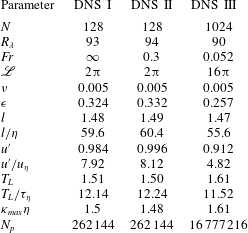
Flow parameters in DNS of isotropic turbulence (arbitrary units).
 $N$
is the number of grid points in each direction,
 $R_{\unicode[STIX]{x1D706}}\equiv u^{\prime }\unicode[STIX]{x1D706}/\unicode[STIX]{x1D708}$
is the Taylor microscale Reynolds number,
 $Fr\equiv \unicode[STIX]{x1D716}^{3/4}/(\unicode[STIX]{x1D708}^{1/4}\mathfrak{g})$
is the Froude number,
 $\mathscr{L}$
is the domain size,
 $\unicode[STIX]{x1D708}$
is the fluid kinematic viscosity,
 $\unicode[STIX]{x1D716}\equiv 2\unicode[STIX]{x1D708}\int _{0}^{\unicode[STIX]{x1D705}_{max}}\unicode[STIX]{x1D705}^{2}E(\unicode[STIX]{x1D705})\,\text{d}\unicode[STIX]{x1D705}$
is the mean turbulent kinetic energy dissipation rate,
 $l\equiv 3\unicode[STIX]{x03C0}/(2k)\int _{0}^{\unicode[STIX]{x1D705}_{max}}E(\unicode[STIX]{x1D705})/\unicode[STIX]{x1D705}\,\text{d}\unicode[STIX]{x1D705}$
is the integral length scale,
 $\unicode[STIX]{x1D702}\equiv \unicode[STIX]{x1D708}^{3/4}/\unicode[STIX]{x1D716}^{1/4}$
is the Kolmogorov length scale,
 $u^{\prime }\equiv \sqrt{(2k/3)}$
is the fluid r.m.s. fluctuating velocity,
 $k$
is the turbulent kinetic energy,
 $u_{\unicode[STIX]{x1D702}}$
is the Kolmogorov velocity scale,
 $T_{L}\equiv l/u^{\prime }$
is the large-eddy turnover time,
 $\unicode[STIX]{x1D70F}_{\unicode[STIX]{x1D702}}\equiv \sqrt{(\unicode[STIX]{x1D708}/\unicode[STIX]{x1D716})}$
is the Kolmogorov time scale,
 $\unicode[STIX]{x1D705}_{max}$
is the maximum resolved wavenumber and
 $N_{p}$
is the number of particles per Stokes number.

Since we want to explore the role of gravity on the small-scale motion of the bidisperse particles, we must consider the choice of
 $Fr$
for the DNS. Observations have shown that
 $\unicode[STIX]{x1D716}$
can vary by orders of magnitude in clouds (Pruppacher & Klett Reference Pruppacher and Klett1997), with corresponding variations in
 $Fr$
. Therefore, in addition to the zero gravity case
 $Fr=\infty$
, we follow Ireland et al. (Reference Ireland, Bragg and Collins2016a
) and consider
 $Fr=0.3,0.052$
, which may be considered to be representative of strongly turbulent cumulonimbus clouds and weakly turbulent stratiform clouds, respectively (Pinsky, Khain & Shapiro Reference Pinsky, Khain and Shapiro2007).
One of the difficulties in simulating very small values of
 $Fr$
is that the use of periodic boundary conditions in the DNS can artificially influence the motion of inertial particles if the DNS box length
 $\mathscr{L}$
is too small. In particular, the use of periodic boundary conditions is problematic if the time it takes the settling particles to traverse the distance
 $\mathscr{L}$
is
 ${\leqslant}O(T_{L})$
. This issue was explored in detail in Ireland et al. (Reference Ireland, Bragg and Collins2016a
) and it was found that box sizes much larger than the standard
 $\mathscr{L}=2\unicode[STIX]{x03C0}$
are needed when
 $Fr$
is very small. For example, in Ireland et al. (Reference Ireland, Bragg and Collins2016a
) it was found that for
 $R_{\unicode[STIX]{x1D706}}\approx 90$
,
 $\mathscr{L}=16\unicode[STIX]{x03C0}$
was necessary, which, with the resolution constraints for accurately resolving the small scales, requires
 $N=1024$
. Such requirements place significant limitations on the value of
 $R_{\unicode[STIX]{x1D706}}$
that can be simulated. In this study we will consider
 $R_{\unicode[STIX]{x1D706}}\approx 90$
, where
 $\mathscr{L}=16\unicode[STIX]{x03C0}$
is used for
 $Fr=0.052$
, whereas the standard size
 $\mathscr{L}=2\unicode[STIX]{x03C0}$
is used for the larger values
 $Fr=\infty ,0.3$
. Although the higher-order statistics of the particle motion are strongly affected by
 $R_{\unicode[STIX]{x1D706}}$
, our recent studies in Ireland et al. (Reference Ireland, Bragg and Collins2016a
,Reference Ireland, Bragg and Collins
b
) showed that at the small scales, the lower-order statistics (e.g. relative velocity variances, collision rates etc.), were insensitive to
 $R_{\unicode[STIX]{x1D706}}$
over the range
 $90\lesssim R_{\unicode[STIX]{x1D706}}\lesssim 600$
when
 $St\leqslant O(1)$
. This justifies the use of the low
 $R_{\unicode[STIX]{x1D706}}$
in this study, but points to the need for future studies to explore the role of
 $R_{\unicode[STIX]{x1D706}}$
on the higher-order statistics of settling, bidisperse particles at the small scales of turbulence.
Details of the DNS are summarized in table 1.
4 Results and discussion
4.1 Relative velocities
We begin by considering results for the relative velocities of the particles. The parallel (longitudinal) and perpendicular (transverse) projections of
 $\boldsymbol{w}^{p}(t)$
are defined as
 $w_{\Vert }^{p}(t)\equiv \boldsymbol{e}_{\Vert }^{p}(t)\boldsymbol{\cdot }\boldsymbol{w}^{p}(t)$
and
 $w_{\bot }^{p}(t)\equiv \boldsymbol{e}_{\bot }^{p}(t)\boldsymbol{\cdot }\boldsymbol{w}^{p}(t)$
, where
 $\boldsymbol{e}_{\Vert }^{p}(t),\boldsymbol{e}_{\bot }^{p}(t)$
are unit vectors parallel and perpendicular to
 $\boldsymbol{r}^{p}(t)$
, respectively.
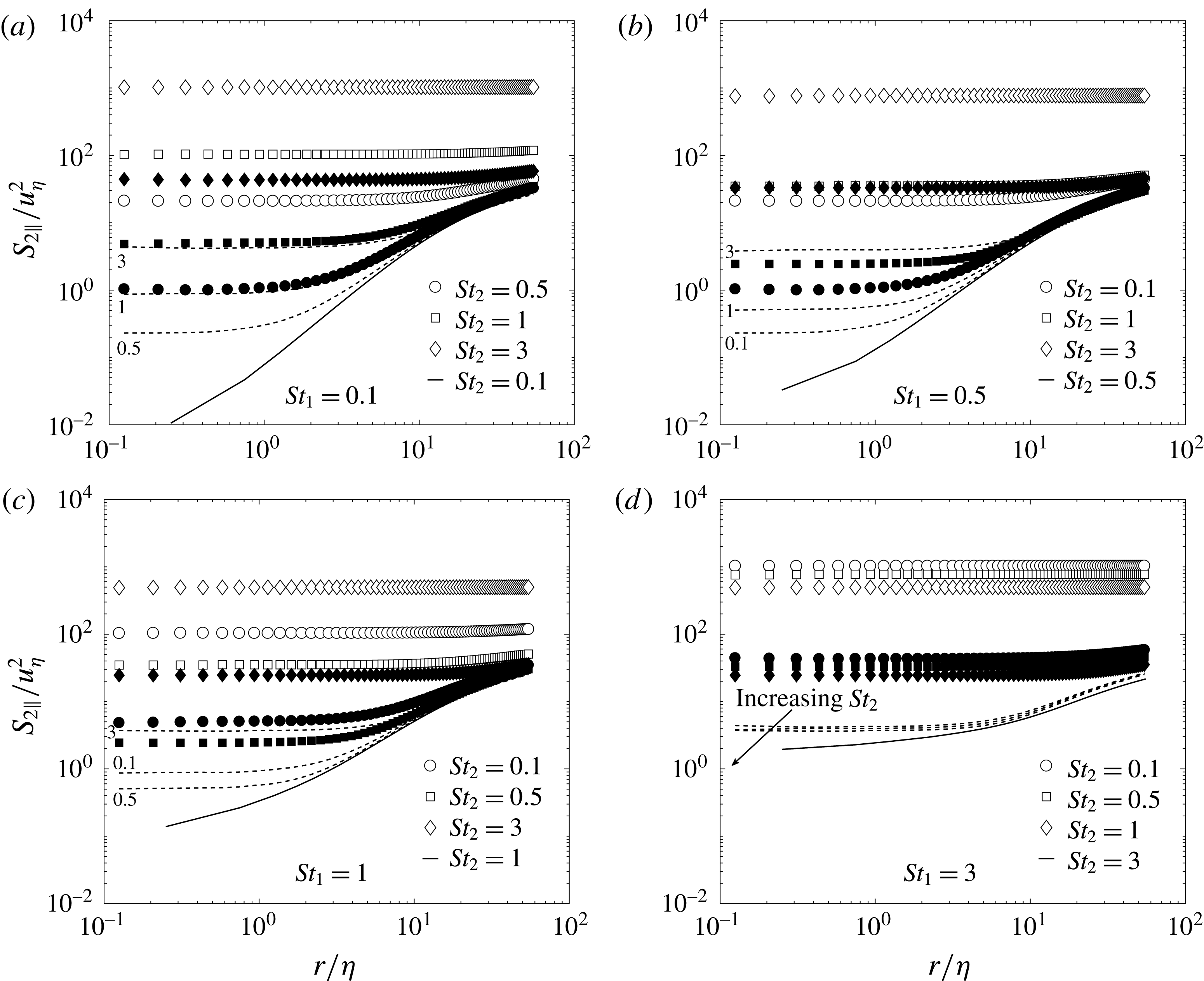
Figure 1 shows the DNS results for the second-order, longitudinal velocity structure function
 $S_{2\Vert }(r)\equiv \langle [w_{\Vert }^{p}(t)]^{2}\rangle _{r}$
, where
 $\langle \cdot \rangle _{r}$
denotes an ensemble average conditioned on
 $\Vert \boldsymbol{r}^{p}(t)\Vert =r$
. We also include the monodisperse results with
 $Fr=\infty$
for comparison. It can be seen that the bidisperse values, with and without gravity, are bounded from below by the monodisperse values. This is in agreement with previous studies that considered bidisperse particle motion without gravitational effects (Zhou et al.
Reference Zhou, Wexler and Wang2001; Zaichik et al.
Reference Zaichik, Simonin and Alipchenkov2006, Reference Zaichik, Fede, Simonin and Alipchenkov2009; Pan & Padoan Reference Pan and Padoan2010; Pan et al.
Reference Pan, Padoan and Scalo2014b
). We also observe in figure 1 that
 $S_{2\Vert }(r)$
becomes independent of
 $r$
at sufficiently small separations. Both of these effects arise because of the acceleration contribution to the bidisperse particle motion, as explained in § 2.
The enhancement of the relative velocities of bidisperse particles at small separations grows as
 $Fr$
is reduced and/or
 $|\unicode[STIX]{x0394}St|$
is increased. For sufficiently large
 $r$
, the effect of the bidispersity weakens, corresponding to the dominance of the first term on the right-hand side of (2.6) at these separations. The results for
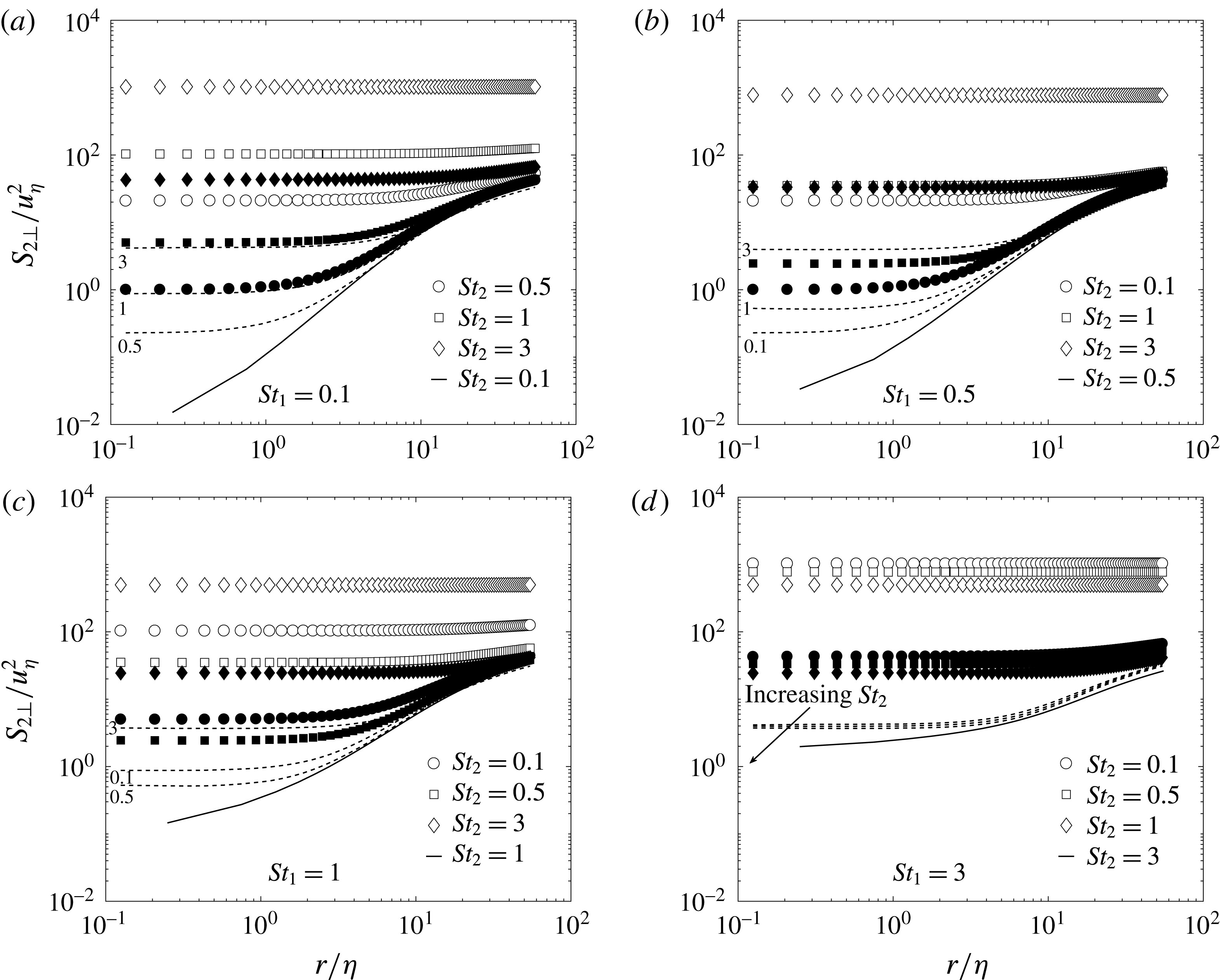
 $S_{2\bot }(r)\equiv \langle [w_{\bot }^{p}(t)]^{2}\rangle _{r},$
are shown in figure 2, which are quantitatively similar to those for
 $S_{2\Vert }(r)$
.
DNS results for
 $S_{2\Vert }/u_{\unicode[STIX]{x1D702}}^{2}$
as a function of
 $r/\unicode[STIX]{x1D702}$
for different
 $St_{1},St_{2},Fr$
combinations. Dashed lines correspond to
 $Fr=\infty$
, filled symbols to
 $Fr=0.3$
, open symbols to
 $Fr=0.052$
and solid lines correspond to the monodisperse case with
 $Fr=\infty$
. The numbers next to the dashed lines indicate the
 $St_{2}$
value that they correspond to.

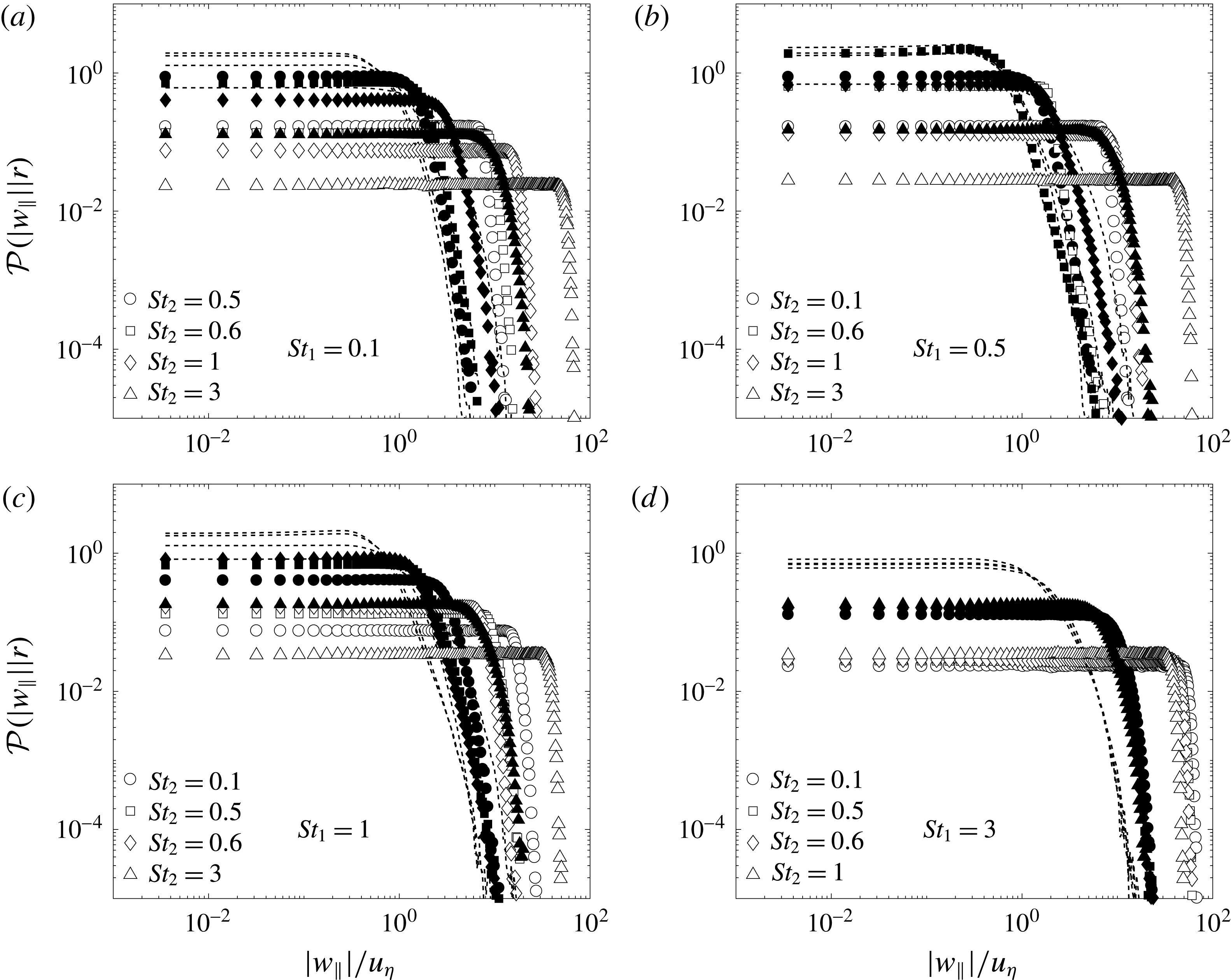
In figure 3 we show results for
 ${\mathcal{P}}(|w_{\Vert }||r)$
, the PDF of the absolute value of the longitudinal relative velocities at separation
 $r$
. As observed by Pan et al. (Reference Pan, Padoan and Scalo2014b
), for
 $Fr=\infty$
, increasing
 $|\unicode[STIX]{x0394}St|$
leads to a broadening of the PDF, corresponding to the enhanced relative velocities through the acceleration effect. Decreasing
 $Fr$
leads to further broadening of the PDF. Most strikingly, when
 $\unicode[STIX]{x0394}St$
is sufficiently large and
 $Fr=0.052$
, the PDF is almost constant up to
 $|w_{\Vert }|\gg u_{\unicode[STIX]{x1D702}}$
and then suddenly reduces. In § 2 we showed that reducing
 $Fr$
can enhance
 $\boldsymbol{w}^{p}(t)$
for bidisperse particles in two ways: explicitly through the differential settling contribution
 $u_{\unicode[STIX]{x1D702}}\unicode[STIX]{x0394}StFr^{-1}\boldsymbol{e}_{\mathfrak{g}}$
, and implicitly through the way that gravity enhances the primary particle acceleration
 $\boldsymbol{a}^{p}$
. Since the orientation of
 $\boldsymbol{r}^{p}(t)$
is time dependent, the effect of gravity on the statistics of the parallel and perpendicular projections of
 $\boldsymbol{w}^{p}(t)$
is not entirely clear, and will involve a mixture of these explicit and implicit effects.
DNS results for
 $S_{2\bot }/u_{\unicode[STIX]{x1D702}}^{2}$
as a function of
 $r/\unicode[STIX]{x1D702}$
for different
 $St_{1},St_{2},Fr$
combinations. Dashed lines correspond to
 $Fr=\infty$
, filled symbols to
 $Fr=0.3$
, open symbols to
 $Fr=0.052$
and solid lines correspond to the monodisperse case with
 $Fr=\infty$
. The numbers next to the dashed lines indicate the
 $St_{2}$
value that they correspond to.

In order to untangle the explicit and implicit effects of gravity on the statistics of
 $\boldsymbol{w}^{p}(t)$
and gain further insight, we consider the second-order structure functions based on the Cartesian components of
 $\boldsymbol{w}^{p}(t)$
. That is, we consider
 $\langle [w_{3}^{p}(t)]^{2}\rangle _{r}$
and
 $\langle [w_{1}^{p}(t)]^{2}\rangle _{r}$
, corresponding to the velocities in the vertical and horizontal directions, respectively (recall also that
 $\langle [w_{1}^{p}(t)]^{2}\rangle _{r}=\langle [w_{2}^{p}(t)]^{2}\rangle _{r}$
due to the axisymmetry of the statistics).
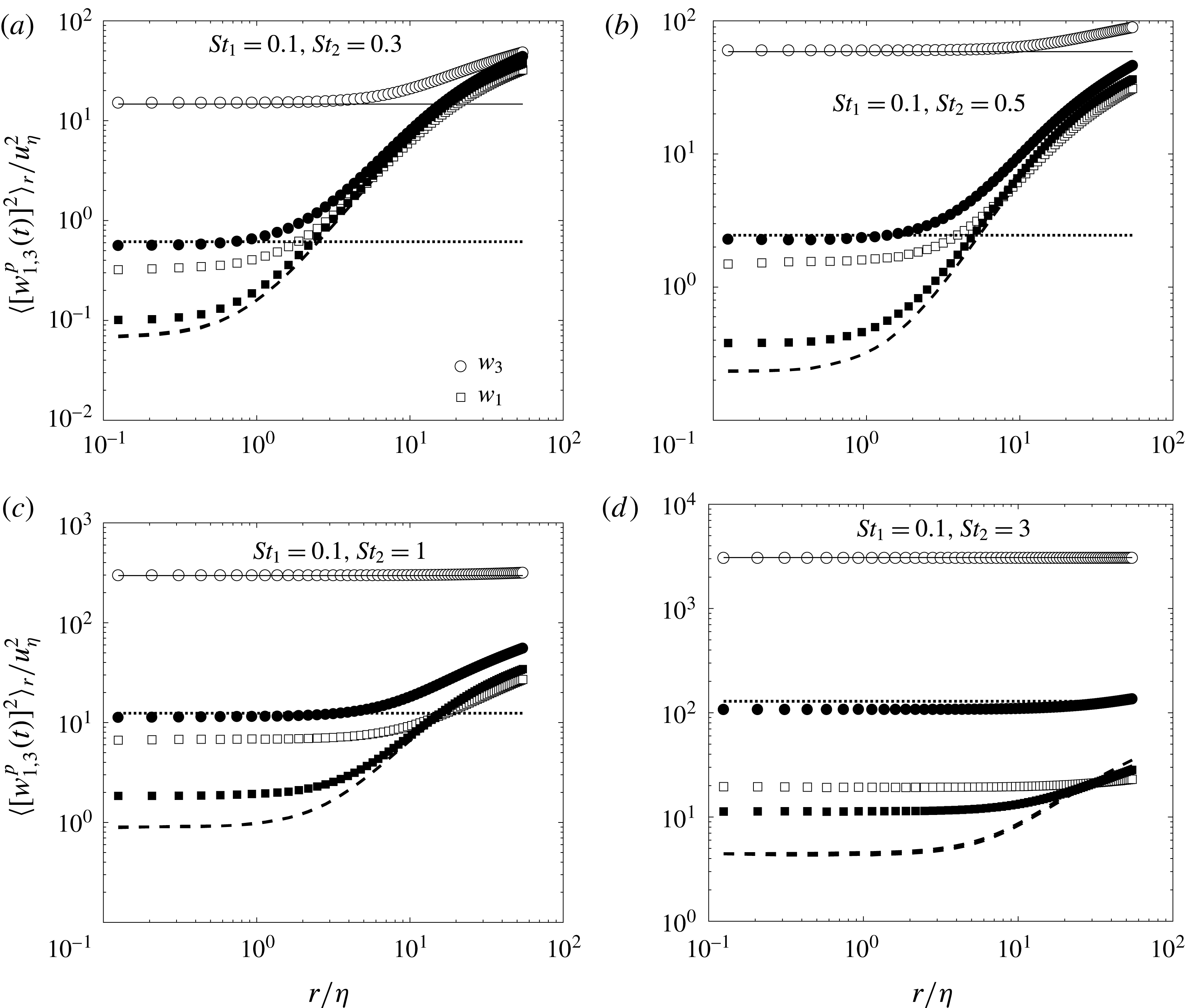
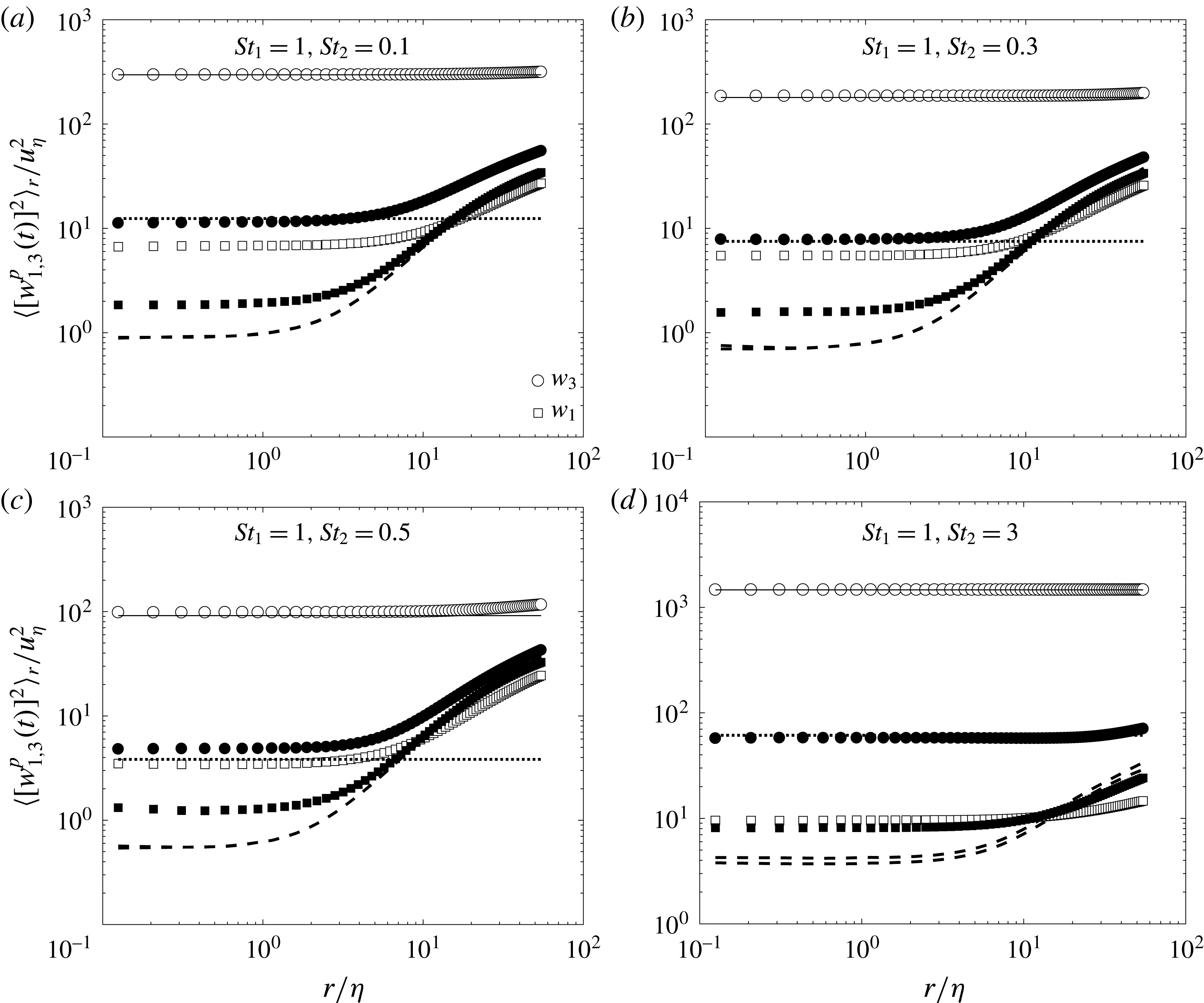
The results are shown in figures 4 and 5, where we also show the
 $Fr\rightarrow 0$
prediction
 $$\begin{eqnarray}\langle [w_{3}^{p}(t)]^{2}\rangle _{r}=\left(u_{\unicode[STIX]{x1D702}}\unicode[STIX]{x0394}StFr^{-1}\right)^{2},\end{eqnarray}$$
which follows from (2.9). When
 $Fr=0.3$
,
 $\langle [w_{3}^{p}(t)]^{2}\rangle _{r}$
is well approximated by (4.1), with some small discrepancies for certain
 $St_{1},St_{2}$
combinations. However, for
 $Fr=0.052$
, (4.1) is in almost perfect agreement with the data for each of the
 $St_{1},St_{2}$
combinations shown. When gravity is active,
 $\langle [w_{3}^{p}(t)]^{2}\rangle _{r}>\langle [w_{1}^{p}(t)]^{2}\rangle _{r}$
, and the difference grows with increasing
 $|\unicode[STIX]{x0394}St|$
and decreasing
 $Fr$
. The analysis in § 2 shows why: as
 $|\unicode[STIX]{x0394}St|$
increases and
 $Fr$
decreases, the contribution to
 $\langle [w_{3}^{p}(t)]^{2}\rangle _{r}$
from the differential settling velocity grows, yet this contribution is absent from
 $\langle [w_{1}^{p}(t)]^{2}\rangle _{r}$
. The results in figures 4 and 5 also show that the implicit effect of gravity can lead to strong enhancements of
 $\langle [w_{1}^{p}(t)]^{2}\rangle _{r}$
, compared with the
 $Fr=\infty$
case, and in some cases the increase corresponds to an order of magnitude. This strong implicit effect of gravity on the horizontal relative velocities could have important implications for understanding and modelling the small-scale mixing and dispersion of bidisperse particles that are settling under gravity.
DNS results for
 ${\mathcal{P}}(|w_{\Vert }||r)$
as a function of
 $|w_{\Vert }|/u_{\unicode[STIX]{x1D702}}$
for different
 $St_{1},St_{2},Fr$
combinations, with
 $r=\unicode[STIX]{x1D702}$
. Dashed lines correspond to
 $Fr=\infty$
, filled symbols to
 $Fr=0.3$
, and open symbols to
 $Fr=0.052$
.

DNS results for
 $\langle [w_{1,3}^{p}(t)]^{2}\rangle _{r}/u_{\unicode[STIX]{x1D702}}^{2}$
as a function of
 $r/\unicode[STIX]{x1D702}$
for
 $St_{1}=0.1$
and different
 $St_{2},Fr$
combinations. Circles correspond to the vertical velocities and squares correspond to the horizontal velocities. Dashed lines correspond to
 $Fr=\infty$
, filled symbols to
 $Fr=0.3$
, open symbols to
 $Fr=0.052$
. The dotted and solid horizontal lines correspond to (4.1) for
 $Fr=0.3$
and
 $Fr=0.052$
, respectively.

DNS results for
 $\langle [w_{1,3}^{p}(t)]^{2}\rangle _{r}/u_{\unicode[STIX]{x1D702}}^{2}$
as a function of
 $r/\unicode[STIX]{x1D702}$
for
 $St_{1}=1$
and different
 $St_{2},Fr$
combinations. Circles correspond to the vertical velocities and squares correspond to the horizontal velocities. Dashed lines correspond to
 $Fr=\infty$
, filled symbols to
 $Fr=0.3$
, open symbols to
 $Fr=0.052$
. The dotted and solid horizontal lines correspond to (4.1) for
 $Fr=0.3$
and
 $Fr=0.052$
, respectively.

DNS results for
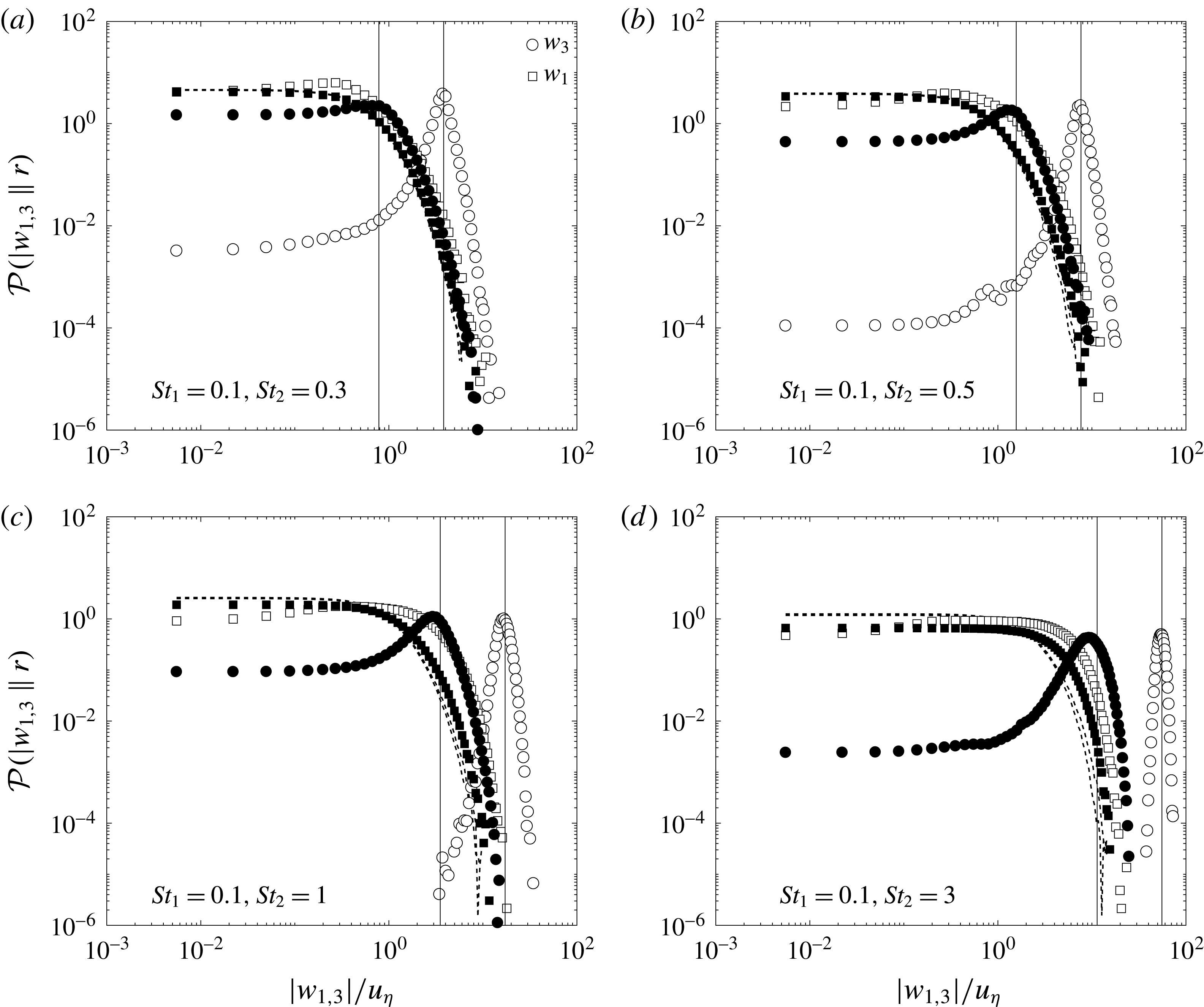
 ${\mathcal{P}}(|w_{1}||r)$
and
 ${\mathcal{P}}(|w_{3}||r)$
as a function of
 $|w_{1,3}|/u_{\unicode[STIX]{x1D702}}$
for
 $St_{1}=0.1$
, different
 $St_{2},Fr$
combinations, and with
 $r=\unicode[STIX]{x1D702}$
. Circles correspond to the vertical velocities and squares correspond to the horizontal velocities. Dashed lines correspond to
 $Fr=\infty$
, filled symbols to
 $Fr=0.3$
, open symbols to
 $Fr=0.052$
. The vertical lines correspond to
 $u_{\unicode[STIX]{x1D702}}|\unicode[STIX]{x0394}St|Fr^{-1}$
for
 $Fr=0.3$
and
 $Fr=0.052$
.

DNS results for
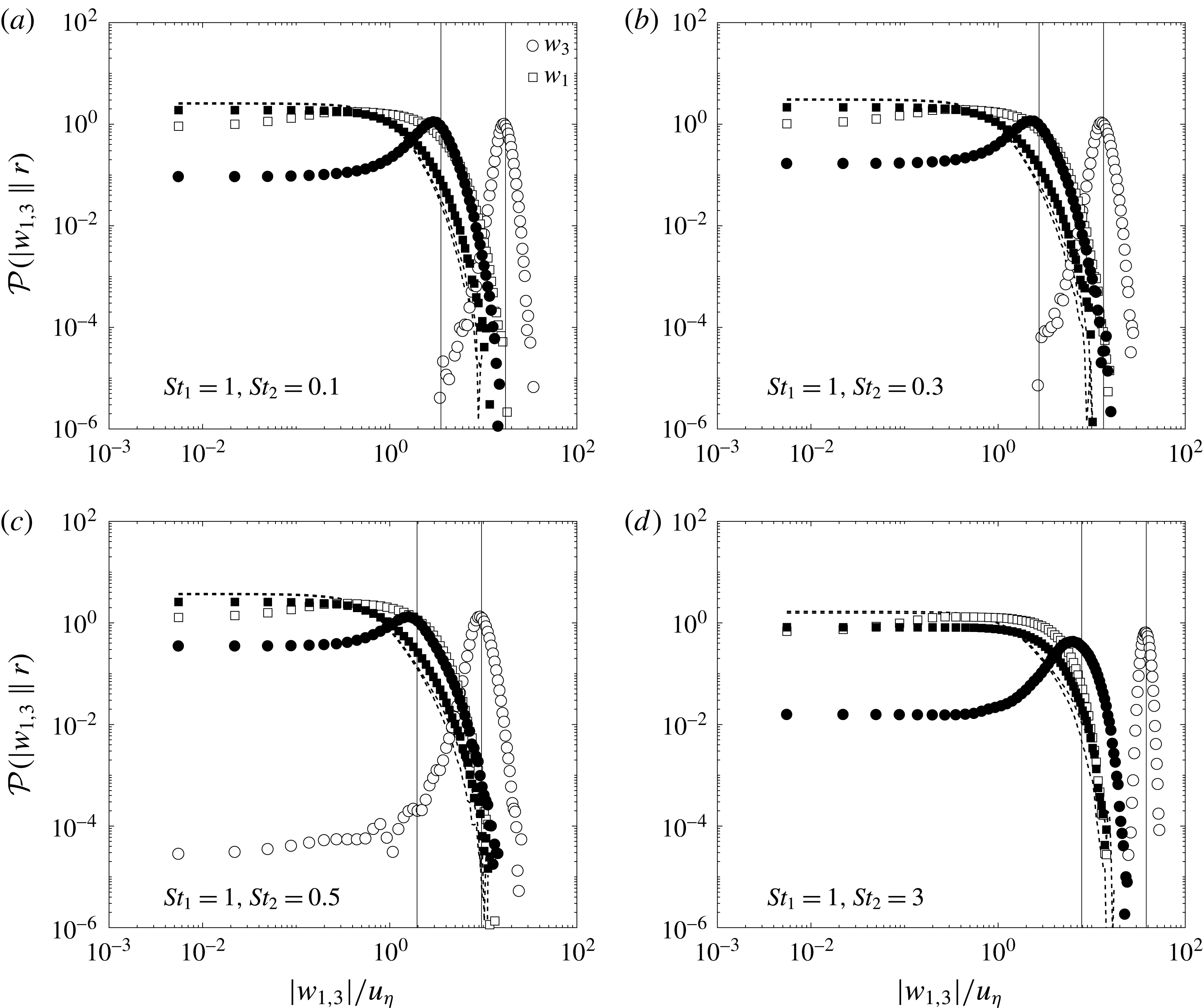
 ${\mathcal{P}}(|w_{1}||r)$
and
 ${\mathcal{P}}(|w_{3}||r)$
as a function of
 $|w_{1,3}|/u_{\unicode[STIX]{x1D702}}$
for
 $St_{1}=1$
, different
 $St_{2},Fr$
combinations, and with
 $r\in [0,2]\unicode[STIX]{x1D702}$
. Circles correspond to the vertical velocities and squares correspond to the horizontal velocities. Dashed lines correspond to
 $Fr=\infty$
, filled symbols to
 $Fr=0.3$
, open symbols to
 $Fr=0.052$
. The vertical lines correspond to
 $u_{\unicode[STIX]{x1D702}}|\unicode[STIX]{x0394}St|Fr^{-1}$
for
 $Fr=0.3$
and
 $Fr=0.052$
.

In figures 6 and 7 we show results for
 ${\mathcal{P}}(|w_{1}||r)$
and
 ${\mathcal{P}}(|w_{3}||r)$
, the PDFs of the absolute value of the horizontal and vertical relative velocities at separation
 $r$
, respectively. As expected, the results show that gravity affects
 ${\mathcal{P}}(|w_{1}||r)$
and
 ${\mathcal{P}}(|w_{3}||r)$
in very different ways, since gravity only plays an explicit role in the vertical direction. Consistent with the results for the structure functions and the arguments of § 2, the PDFs for the horizontal velocities shift towards larger values, corresponding to the enhancement arising from the implicit effect of gravity. For the vertical velocities, the mode of the PDF is close to
 $u_{\unicode[STIX]{x1D702}}|\unicode[STIX]{x0394}St|Fr^{-1}$
, which is indicated by the vertical lines in figures 6 and 7. However, only for
 $|\unicode[STIX]{x0394}St|>2$
and
 $Fr=0.052$
does the PDF approach the asymptotic behaviour
 $$\begin{eqnarray}\lim _{Fr\rightarrow 0}{\mathcal{P}}(|w_{3}||r)\rightarrow \unicode[STIX]{x1D6FF}\left(u_{\unicode[STIX]{x1D702}}|\unicode[STIX]{x0394}St|Fr^{-1}-|w_{3}|\right).\end{eqnarray}$$
When
 $Fr=0.052$
, the explicit effect of gravity was shown to dominate
 $\langle [w_{3}^{p}(t)]^{2}\rangle _{r}$
, even when
 $|\unicode[STIX]{x0394}St|<1$
. However, the results in figures 6 and 7 show that for the same parameter range,
 ${\mathcal{P}}(|w_{3}||r)$
is not dominated by the gravity asymptote, implying that
 $\langle [w_{3}^{p}(t)]^{n}\rangle _{r}=(u_{\unicode[STIX]{x1D702}}\unicode[STIX]{x0394}StFr^{-1})^{n}$
can fail for
 $n\neq 2$
. We would also expect the deviation from (4.2) to increase as
 $R_{\unicode[STIX]{x1D706}}$
is increased due to the enhanced intermittency in the turbulence, since the probability of the terms involving
 $\unicode[STIX]{x0394}u_{3}^{p}$
and
 $a_{3}^{p}$
becoming comparable to
 $u_{\unicode[STIX]{x1D702}}\unicode[STIX]{x0394}StFr^{-1}$
in the equation for
 $w_{3}^{p}(t)$
would increase. This implies that in applications such as clouds where
 $R_{\unicode[STIX]{x1D706}}=O(10^{4})$
(Grabowski & Wang Reference Grabowski and Wang2013), the asymptotic behaviour (4.2) may never be realized due to the extremely small values of
 $Fr$
that would be required. This could have important implications for understanding and modelling the vertical mixing of settling, bidisperse particles in a variety of turbulent flows.
4.2 Spatial clustering
We now turn to consider the spatial clustering of the particles, which may be quantified using the radial distribution function (RDF), defined as (McQuarrie Reference McQuarrie1976)
 $$\begin{eqnarray}g(r)\equiv \frac{N_{i}/\unicode[STIX]{x1D6FF}V_{i}}{N_{1}N_{2}/V}.\end{eqnarray}$$
If we define the number of satellite particles (with Stokes number
 $St_{2}$
) found at a distance
 $r$
from a given primary particle (with Stokes number
 $St_{1}$
) to be
 $N_{i}^{\prime }$
, then
 $N_{i}$
is the sum of
 $N_{i}^{\prime }$
over all primary particles in the system.
 $\unicode[STIX]{x1D6FF}V_{i}$
is the volume of an elemental spherical shell with surface at a distance
 $r$
from the primary particle,
 $V$
is the total volume of the system and
 $N_{1}$
and
 $N_{2}$
are the total numbers of primary and satellite particles in the domain, respectively. Note that the RDF is the same (to within a constant) as
 $\Vert \boldsymbol{r}\Vert ^{-2}$
times the spherical average of the PDF
 $\unicode[STIX]{x1D711}(\boldsymbol{r})$
introduced in § 2.
DNS results for
 $g(r)$
as a function of
 $r/\unicode[STIX]{x1D702}$
for different
 $St_{1},St_{2},Fr$
combinations. Dashed lines correspond to
 $Fr=\infty$
, filled symbols to
 $Fr=0.3$
, open symbols to
 $Fr=0.052$
and solid lines correspond to the monodisperse case with
 $Fr=\infty$
. The numbers next to the dashed lines indicate the
 $St_{2}$
value that they correspond to.

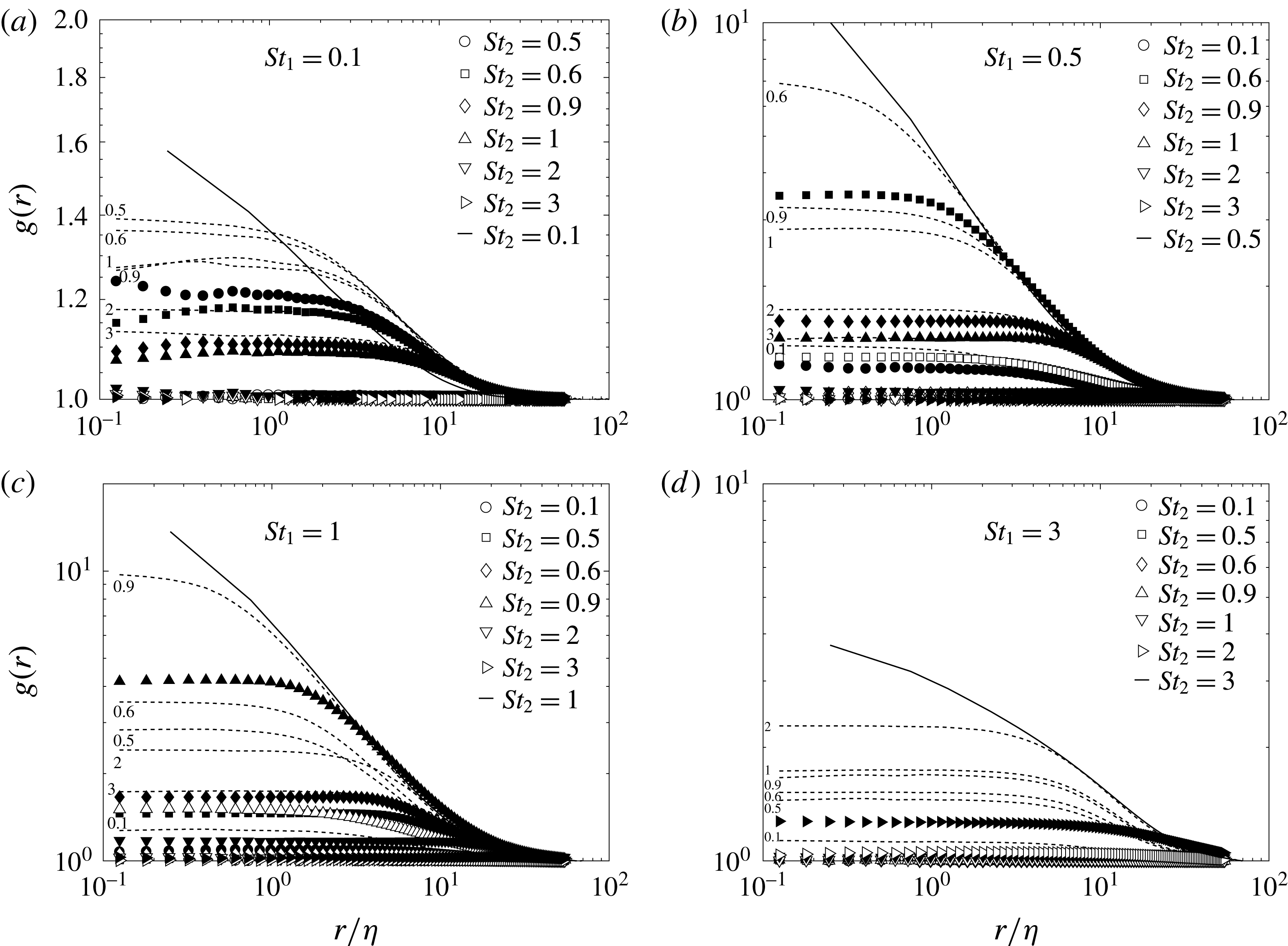
The results in figure 8 show that in general, increasing
 $|\unicode[STIX]{x0394}St|$
reduces the RDF, and that the clustering is significantly reduced for
 $r/\unicode[STIX]{x1D702}\ll 1$
even when
 $|\unicode[STIX]{x0394}St|\ll 1$
. These results for
 $Fr=\infty$
are consistent with previous investigations (Zhou et al.
Reference Zhou, Wexler and Wang2001; Chun et al.
Reference Chun, Koch, Rani, Ahluwalia and Collins2005; Pan et al.
Reference Pan, Padoan, Scalo, Kritsuk and Norman2011). This reduction is consistent with the explanations in § 2, namely, that the acceleration contribution to the relative motion of bidisperse particles leads to an enhanced particle-pair diffusion and reduced inward drift, leading to reduced clustering, and to a plateau of the RDF at small separations.
We also note that although the RDF at
 $r/\unicode[STIX]{x1D702}\leqslant 1$
is always largest for
 $\unicode[STIX]{x0394}St=0$
, i.e. the monodisperse case, the same is not always true at larger separations (e.g. see figure 8
a). Over the
 $St_{1},St_{2}$
range we are here considering,
 $|\unicode[STIX]{x0394}St|>0$
monotonically increases the particle-pair diffusion tensor, and therefore, this behaviour must be caused by bidispersity leading to an enhancement of the inward drift term
 $St_{2}\unicode[STIX]{x1D711}\unicode[STIX]{x1D735}_{\boldsymbol{r}}\boldsymbol{\cdot }\langle w_{1}^{p}(t)\boldsymbol{w}^{p}(t)\rangle _{\boldsymbol{r}}$
in (2.18) in certain regimes of
 $St_{1},St_{2}$
.
In agreement with the arguments in § 2, the results in figure 8 also show that decreasing
 $Fr$
further suppresses the clustering of bidisperse particles. Indeed, even for
 $|\unicode[STIX]{x0394}St|=0.1$
, gravity is very effective at suppressing the clustering.
DNS results for
 $g(r)$
as a function of
 $St_{2}$
, at specific values of
 $r/\unicode[STIX]{x1D702}$
and for different
 $St_{1},Fr$
combinations. Dashed lines correspond to
 $Fr=\infty$
, filled symbols to
 $Fr=0.3$
, open symbols to
 $Fr=0.052$
.

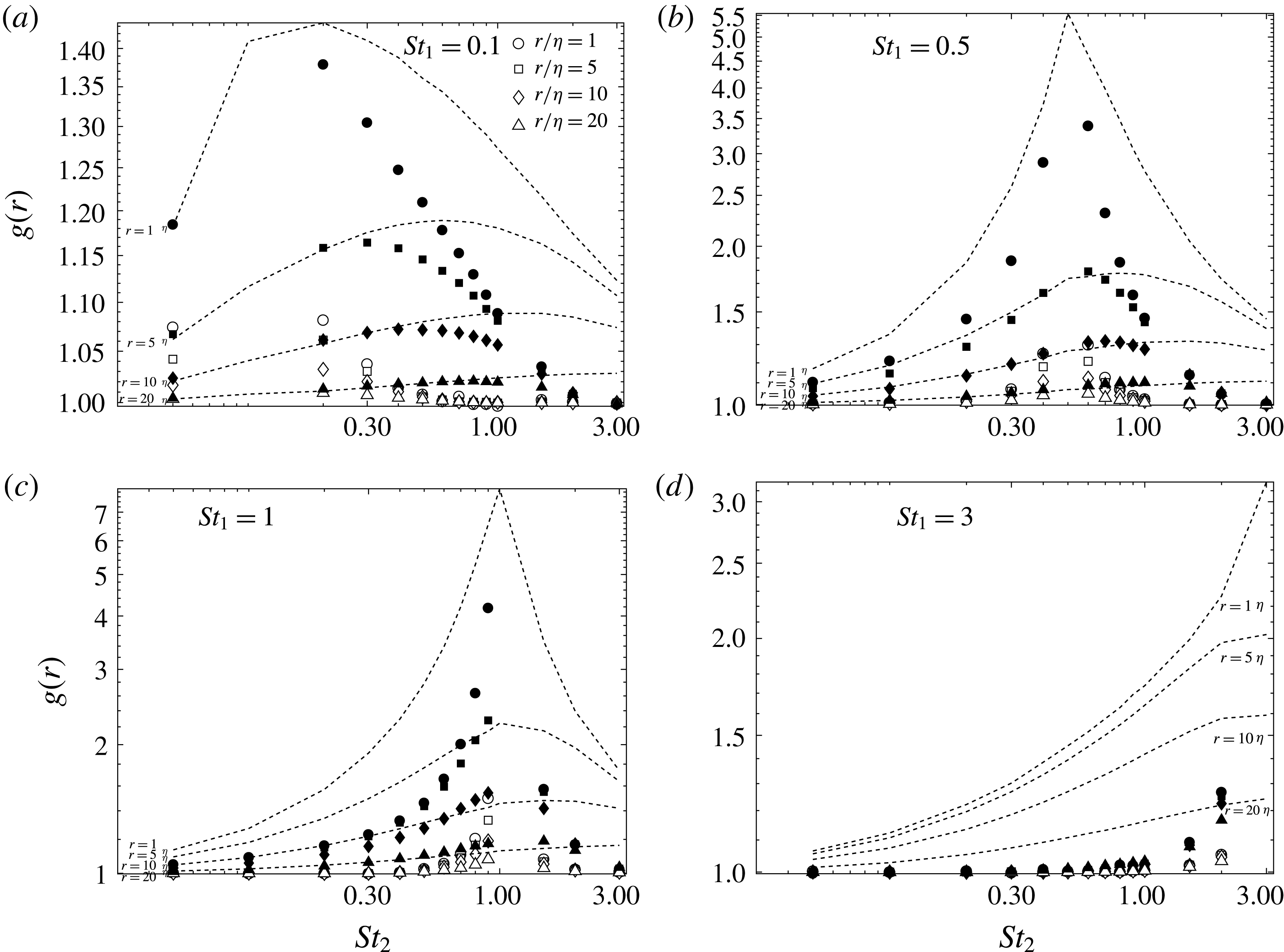
To see more clearly the effect of bidispersity and gravity on the RDF, in figure 9 we plot the RDF for a given
 $St_{1}$
as a function of
 $St_{2}$
at four different separations. As discussed earlier, the results show that the bidisperse RDFs generally peak when the difference between
 $St_{1}$
and
 $St_{2}$
is smallest. Figure 9 also shows more clearly how gravity systematically suppresses the clustering over the range of
 $St,\unicode[STIX]{x0394}St,Fr$
considered. This is in contrast to the monodisperse case for which it has been observed that gravity can actually enhance clustering in certain regimes of
 $St,Fr$
(Bec et al.
Reference Bec, Homann and Ray2014; Gustavsson et al.
Reference Gustavsson, Vajedi and Mehlig2014; Ireland et al.
Reference Ireland, Bragg and Collins2016b
). We expect that this enhancement could also be observed for bidisperse particles when
 $St_{2}>1$
if
 $|\unicode[STIX]{x0394}St|\ll 1$
. However, we do not have data for this regime, although it is something that should be investigated in future work. Also, the regime
 $Fr=O(1)$
should also be explored in future work to see if the clustering enhancement is observed for bidisperse particles in that regime.
We add the cautionary remark that when we used a box length of
 $2\unicode[STIX]{x03C0}$
for the
 $Fr=0.052$
case, we observed that the RDF was larger than for the
 $Fr=0.3$
case, giving the appearance of enhanced clustering due to gravity. However, this apparent enhancement disappeared for the much larger box length of
 $16\unicode[STIX]{x03C0}$
used in this study. This highlights the need to use large computational domains when
 $Fr\ll 1$
in order to ensure the dynamics of the settling particles is not artificially affected by the periodic boundary conditions used in the DNS, as discussed in detail in Ireland et al. (Reference Ireland, Bragg and Collins2016b
).
4.3 Collision kernel
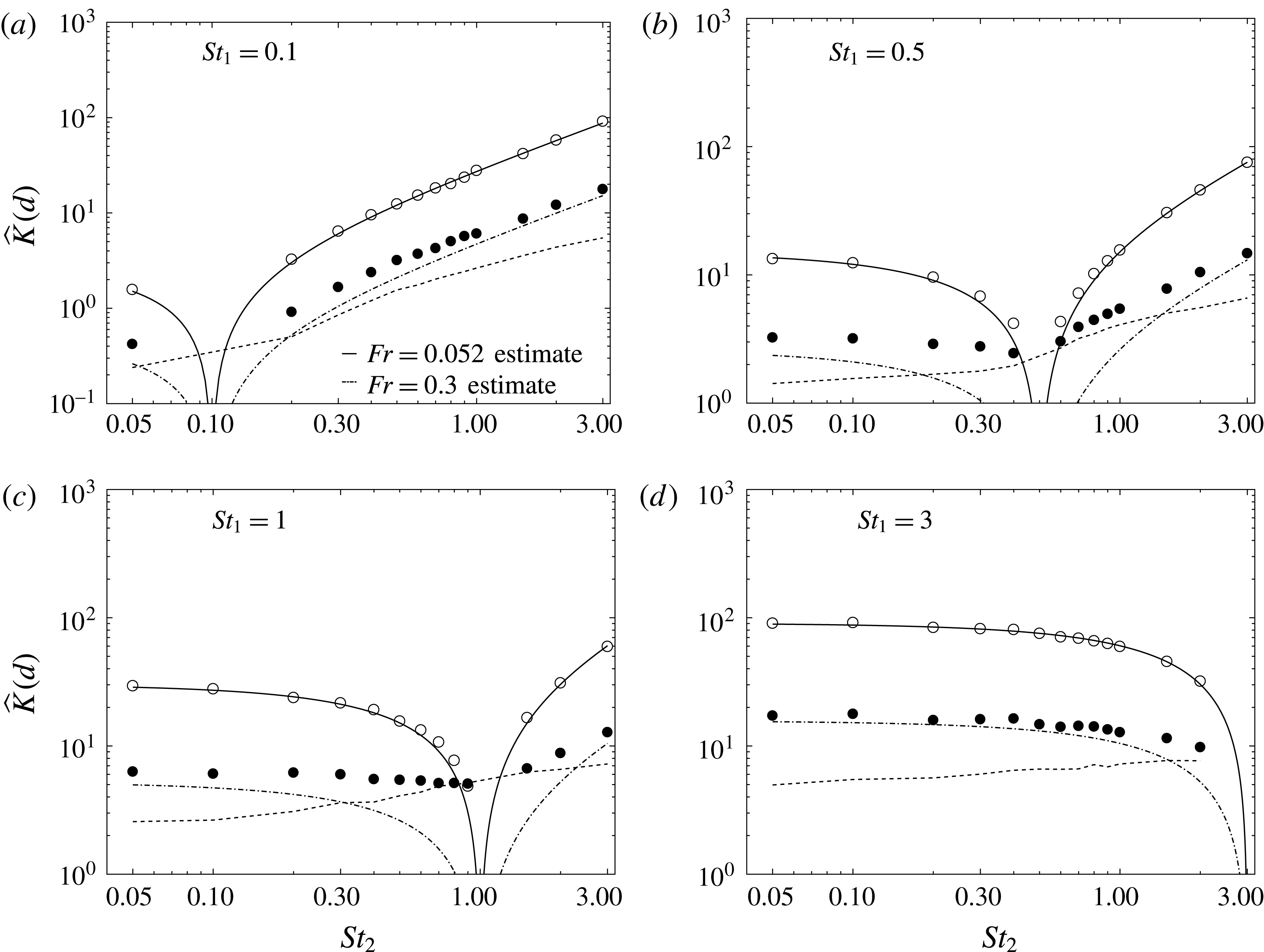
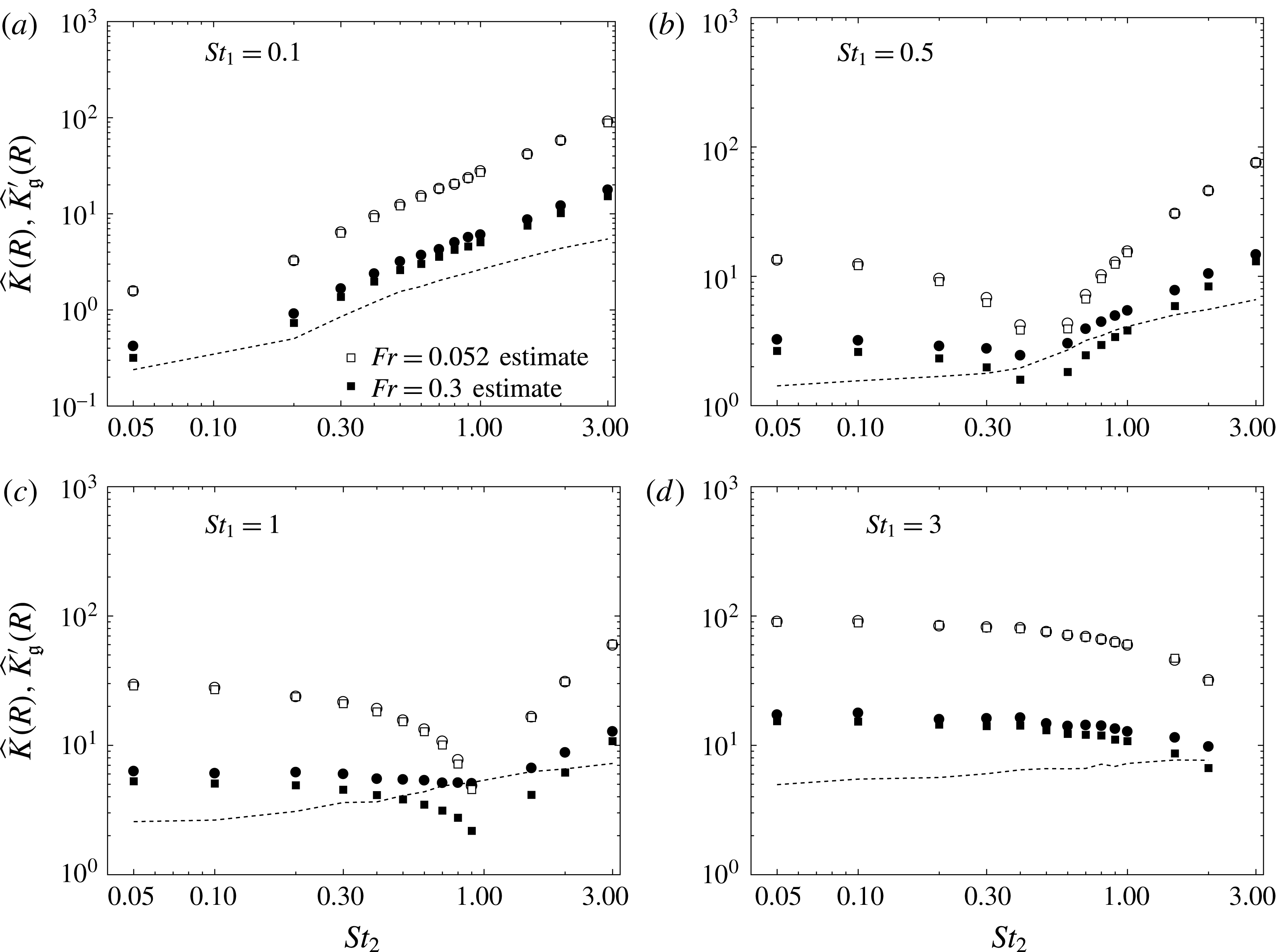
Finally, we consider the collision kernel for the bidisperse particles. The collision kernel is given by (Sundaram & Collins Reference Sundaram and Collins1997)
 $$\begin{eqnarray}K(d)\equiv 4\unicode[STIX]{x03C0}d^{2}g(d)S_{-\Vert }(d),\end{eqnarray}$$
where
 $d\equiv (d_{1}+d_{2})/2$
is the collision diameter of two spherical particles with diameters
 $d_{1}$
and
 $d_{2}$
, and
 $S_{-\Vert }(r)\equiv \langle w_{\Vert }^{p}(t)|<0\rangle _{r}$
is the average of
 $w_{\Vert }^{p}(t)$
conditioned on
 $w_{\Vert }^{p}(t)<0$
for the separation
 $r$
(i.e. the mean inward relative velocity).
In Ireland et al. (Reference Ireland, Bragg and Collins2016a
,Reference Ireland, Bragg and Collins
b
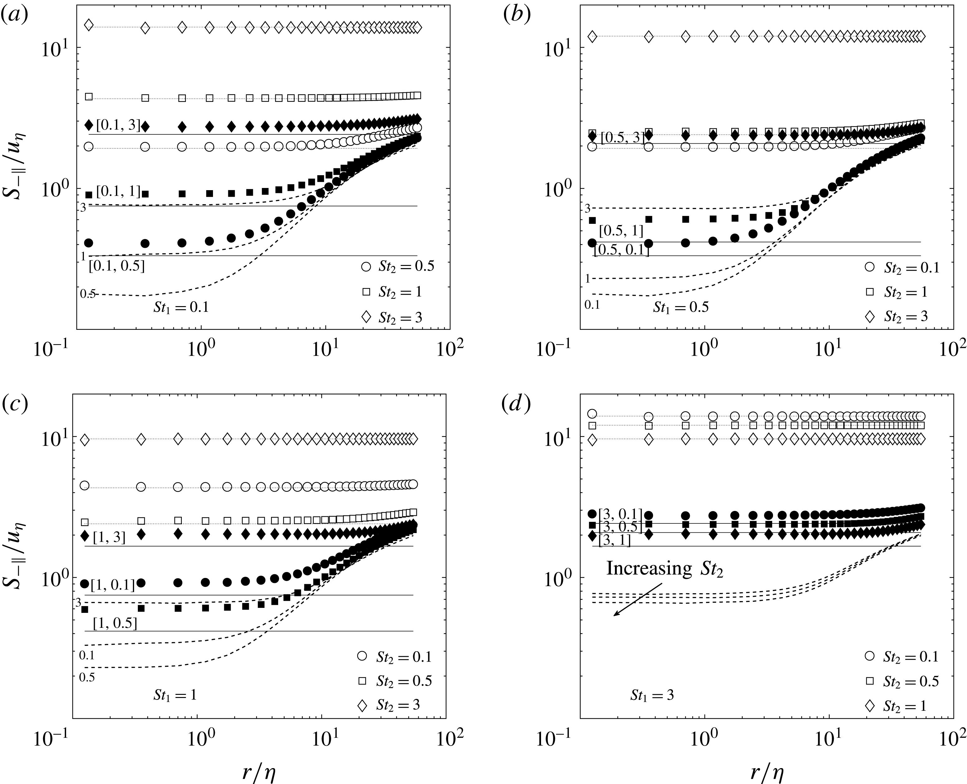
), when plotting
 $K(d)$
we chose a fluid to particle density ratio, for which
 $d$
is then determined by
 $St$
. Since
 $d$
so determined is often smaller than the smallest separation for which we have data for
 $g$
and
 $S_{-\Vert }$
, we had to extrapolate our DNS data down to
 $d$
. For the monodisperse case considered in Ireland et al. (Reference Ireland, Bragg and Collins2016a
,Reference Ireland, Bragg and Collins
b
), this was justified since the functional forms of
 $g$
and
 $S_{-\Vert }$
are known at small separations, i.e. they are power laws (Gustavsson & Mehlig Reference Gustavsson and Mehlig2011). However, in the bidisperse case, and with gravity, we do not know how
 $g$
and
 $S_{-\Vert }$
depend upon
 $r$
(they are not power laws), and therefore extrapolation would be unreliable. Therefore, we will simply consider
 $K(d=0.125\unicode[STIX]{x1D702})$
, corresponding to the smallest separation at which our DNS data are reliable.
In figure 10 we show results for the normalized collision kernel
 $\widehat{K}(d)\equiv K(d)/(d^{2}u_{\unicode[STIX]{x1D702}})$
. The results show that decreasing
 $Fr$
enhances
 $\widehat{K}(d)$
; since clustering reduces as
 $Fr$
is decreased, this enhancement arises solely because of the enhanced relative velocities due to gravity. Also shown in the plot is the collision kernel for settling bidisperse particles in quiescent flow (Grabowski & Wang Reference Grabowski and Wang2013)
 $$\begin{eqnarray}K_{\mathfrak{g}}(d)=\unicode[STIX]{x03C0}d^{2}|\unicode[STIX]{x0394}St|Fr^{-1}u_{\unicode[STIX]{x1D702}}.\end{eqnarray}$$
The results show that for
 $Fr=0.052$
,
 $K_{\mathfrak{g}}(d)$
is in excellent agreement with
 $K(d)$
. As we demonstrated earlier, turbulence plays a very significant role on the horizontal relative velocities even when
 $Fr\ll 1$
; however, the relative velocities in the vertical direction are in general much larger, and so the vertical relative velocities dominate the behaviour of
 $S_{-\Vert }(d)$
. For
 $Fr=0.3$
,
 $K_{\mathfrak{g}}(d)$
is in reasonable agreement with
 $K(d)$
only if
 $|\unicode[STIX]{x0394}St|\gtrsim 1$
, and in general
 $K_{\mathfrak{g}}(d)$
significantly underpredicts
 $K(d)$
.
To determine the cause of this underprediction, in figure 11 we plot
 $\widehat{K}_{\mathfrak{g}}^{\prime }(d)=\unicode[STIX]{x03C0}g(d)|\unicode[STIX]{x0394}St|Fr^{-1}$
, which uses the DNS data for
 $g(d)$
, but the gravity estimate for
 $S_{-\Vert }(d)$
. The results show that for
 $Fr=0.052$
,
 $\widehat{K}_{\mathfrak{g}}^{\prime }(d)\approx \widehat{K}_{\mathfrak{g}}(d)\approx \widehat{K}(d)$
since the particle clustering is almost absent. However, for
 $Fr=0.3$
,
 $\widehat{K}_{\mathfrak{g}}^{\prime }(d)$
provides a significantly improved prediction for
 $\widehat{K}(d)$
compared with
 $\widehat{K}_{\mathfrak{g}}(d)$
, implying the importance of clustering on the collisions rates in this regime. However, for some combinations of
 $St_{1},St_{2}$
,
 $\widehat{K}_{\mathfrak{g}}^{\prime }(d)$
still underpredicts
 $K(d)$
which must be due to errors in the gravity estimate
 $S_{-\Vert }(r)=(1/4)u_{\unicode[STIX]{x1D702}}/|\unicode[STIX]{x0394}St|Fr^{-1}$
.
DNS results for
 $\widehat{K}(d)$
as a function of
 $St_{2}$
, for
 $d=0.125\unicode[STIX]{x1D702}$
and for different
 $St_{1},Fr$
combinations. Dashed lines correspond to
 $Fr=\infty$
, filled symbols to
 $Fr=0.3$
, open symbols to
 $Fr=0.052$
. The dashed-dot and solid lines correspond to the predictions of (4.5) for
 $Fr=0.3$
and
 $Fr=0.052$
, respectively.

DNS results for
 $\widehat{K}$
(circles) and
 $\widehat{K}_{\mathfrak{g}}^{\prime }$
(squares) as a function of
 $St_{2}$
, for
 $d=0.125\unicode[STIX]{x1D702}$
and for different
 $St_{1},Fr$
combinations. Dashed lines correspond to
 $Fr=\infty$
, filled symbols to
 $Fr=0.3$
, open symbols to
 $Fr=0.052$
.

In figure 12 we plot the DNS data for
 $S_{-\Vert }(r)$
and compare the results with the gravity estimate. As anticipated, the results show that whereas the gravity estimate
 $$\begin{eqnarray}S_{-\Vert }(r)=(1/4)u_{\unicode[STIX]{x1D702}}/|\unicode[STIX]{x0394}St|Fr^{-1}\end{eqnarray}$$
is in excellent agreement with the DNS data for
 $Fr=0.052$
and
 $r<\unicode[STIX]{x1D702}$
, it underpredicts the DNS data for
 $Fr=0.3$
for some combinations of
 $St_{1},St_{2}$
.
DNS results for
 $S_{-\Vert }(r)$
as a function of
 $r/\unicode[STIX]{x1D702}$
, for different
 $St_{1},St_{2},Fr$
combinations. Dashed lines correspond to
 $Fr=\infty$
, filled symbols to
 $Fr=0.3$
, open symbols to
 $Fr=0.052$
. The numbers next to the dashed lines indicate the
 $St_{2}$
value that they correspond to. The dotted lines correspond to the predictions of (4.6) for
 $Fr=0.052$
, and the solid lines correspond to the predictions of (4.6) for
 $Fr=0.3$
, where the
 $St_{1},St_{2}$
combinations that the lines correspond to are shown in square brackets for clarity.

5 Conclusions
We have used DNS to explore the relative motion of settling, bidisperse inertial particles at the small scales of isotropic turbulence. We found that gravity can strongly enhance the relative velocities of the particles, not only in the direction of gravity, but also in the direction normal to its action. When
 $Fr\ll 1$
the PDF of the relative velocity in the direction of gravity has a mode that is well described by the differential settling velocity; however, unless the difference in the Stokes number of the two particles is
 ${\geqslant}O(1)$
, the PDF can have a significant spread around this value. These findings are very important for the vertical and horizontal mixing of settling, bidisperse particles in turbulence since it implies that even for
 $Fr\ll 1$
, their vertical mixing rates are not necessarily dominated by gravity, but that turbulence can continue to play a strong role, and further, that their horizontal mixing due to turbulence can be significantly enhanced by gravity.
We find that for the range of
 $St_{2}$
and
 $\unicode[STIX]{x0394}St$
considered, gravity always suppresses the clustering of bidisperse particles in turbulence, in contrast to the monodisperse case where it can strongly enhance it. Indeed, for
 $Fr=0.052$
, the particles are almost uniformly distributed throughout the flow for the range of
 $St$
and
 $\unicode[STIX]{x0394}St$
considered.
Finally, we considered the collision rates of the particles. We found that gravity strongly enhances the collision rates of bidisperse particles, due to their enhanced relative velocities, both in the direction of and normal to gravity. For
 $Fr=0.3$
, the collision kernel prediction based on settling bidisperse particles in quiescent flow underpredicts the DNS data except for
 $|\unicode[STIX]{x0394}St|>1$
, but is in near perfect agreement for
 $Fr=0.052$
, even for
 $0<|\unicode[STIX]{x0394}St|\ll 1$
.
As discussed earlier, one of the primary reasons for considering a bidisperse system is that in clouds and many other problems, particle collisions are usually binary due to the dilute particle loading (Grabowski & Wang Reference Grabowski and Wang2013). In such a case, the problem of polydispersity reduces to understanding the effect of bidispersity on the particle-pair motion, since the polydisperse statistics can be obtained through suitable integrals of the bidisperse statistics, weighted according to the size distribution of the particles. In other situations, such as when the particle loading is not sufficiently dilute, it can be important to directly understand the full polydisperse behaviour. However, a study of the effect of polydispersity on the small-scale dynamics of settling particles in turbulence is beyond the scope of the present work, but must be considered in the future.
In conclusion, these results have shown how gravity leads to a number of interesting effects on the dynamics of bidisperse particles at the small scales of turbulence, and that turbulence plays a crucial role in the particle motion even when
 $Fr\ll 1$
. A key point is that
 $Fr$
only characterizes the importance of gravity compared with some typical r.m.s. acceleration of the fluid. However, in turbulence the acceleration is extremely intermittent when
 $R_{\unicode[STIX]{x1D706}}$
is large. As a consequence, there is a significant probability for particles to be in regions of the flow where the local, instantaneous Froude number is
 ${>}1$
, even though the typically defined Froude number is
 $\ll 1$
. This could imply, for example, that extreme events in the mixing of settling, bidisperse particles are weakly affected by gravity even when
 $Fr\ll 1$
. To investigate these issues, it is important in future studies to consider higher
 $R_{\unicode[STIX]{x1D706}}$
than we have studied. A significant challenge in this respect is the large computational domains required when
 $Fr\ll 1$
.
Acknowledgement
We gratefully acknowledge P. J. Ireland for providing some of the data used in this paper.