NOMENCLATURE
 $p, q, r$
angular rate along x, y, z axis
- $X_{ay}, Y_{ay}, Z_{ay}$
sensor offset for accelerometer
- EKF
extended Kalman filter
- UKF
unscented Kalman filter
- P
state propagation error covariance matrix
- Q
process noise covariance matrix
- R
measurement noise covariance matrix
- F
state noise distribution matrix
- $V_{0}$
initial velocity of aircraft
- $I_{(.)}$
product of inertia
- $C_{y}$
lateral force coefficient
- $ C_{l}$
rolling moment coefficient
- $ C_{n}$
yawing moment coefficient
- $C_{y(\cdot )}, C_{l(\cdot }), C_{n(\cdot )}$
aerodynamic derivatives


Greek symbols
- $\alpha$
angle-of-attack
- $\beta$
angle of sideslip
- $\theta$
pitch angle
- $\phi$
bank angle


1.0 INTRODUCTION
The estimation of aircraft stability and control parameters in the lateral directions is a challenging task due to the coupled motion produced by the interaction between the yawing and rolling motions. Parameter estimation is an essential step in the modelling and analysis of an aircraft to obtain a valid mathematical model for the design of flight control laws, verification of performance predictions and implementations of flight simulation(Reference Tischler and Remple1,Reference Jategaonkar2) . The set of differential equations describing the mathematical model of an aircraft contains force and moment coefficients. Furthermore, each coefficient is represented in terms of parameters associated with the stability and control of the aircraft(Reference Nelson3). Estimation of such parameters for an aircraft system invites the use of an appropriate estimator that can handle both the noise and non-linearity present in the system dynamics.
As far as the estimation algorithm is concerned, a simple Output Error Method (OEM) in the framework of a deterministic system is found to be adequate in many practical cases(Reference Morelli and Klein4). Thus, the investigation of aircraft parameters is primarily addressed by the maximum-likelihood method with the application of the OEM(Reference Ljung5–Reference Iliff7). In the context of process noise, the Filter Error Method (FEM) is an alternative approach for parameter estimation(Reference Grauer and Morelli8). However, for the online estimation of aerodynamic parameters, the Extended Kalman Filter (EKF) is widely used by linearising the non-linear aircraft system(Reference Simon9). Intuitively, if the a priori estimation is far from the actual state, the linearisation around the estimate introduces an error into the estimation. Moreover, the EKF is hard to tune and implement when dealing with significant non-linearities and exhibits divergence in estimates. In contrast, the Unscented Kalman Filter (UKF) uses as a non-linear filter without linearising the non-linear model(Reference Julier and Uhlmann10). Data-driven methods such as Neural Partial Differentiation (NPD)(Reference Sinha, Kuttieri and Chatterjee11–Reference Mohamed and Dongare13), the Genetic Algorithm (GA) and Particle Swarm Optimization (PSO) are also used for parameter estimation(Reference Roy and Peyada14–Reference Alireza16). However, these black-box modelling techniques suffer from the drawback of requiring training with a large number of datasets and longer computational time.
The rapid variations of aerodynamic parameters during the manoeuvring of an aircraft require an online estimation algorithm for handling this highly non-linear system. The use of the UKF appears appropriate for the aircraft dynamics of a non-linear system for identifying parameters in real time. However, the design of the UKF faces difficulty in tuning the proper values of process and measurement covariance matrices Q and R, respectively, failure of which can lead to divergence of the filter. The presence of external disturbances such as wind or turbulence causes considerable variation in the aircraft dynamics and concern regarding the adaptive regulation of the noise covariance matrices Q and R(Reference Gao, Gao, Hu, Zhong and Gu17–Reference Majeed and Kar19). This article proposes an adaptive stochastic non-linear filter (ASNF) for the estimation of the lateral directional aerodynamic parameters. The proposed algorithm considers covariance matching techniques for the adaptation of noise statistics as well as unscented transformation for the non-linear system dynamics of the aircraft.
2.0 AIRCRAFT LATERAL DIRECTIONAL MODEL FOR PARAMETER ESTIMATION
The lateral directional motion in an aircraft response can be represented by the following postulated aircraft state models(Reference Klein and Moreli20):
 \begin{equation} \left\{ \begin{array}{l} \dot \beta = \frac{{\bar qs}}{{m{V_0}}}{C_y}\cos \beta + p\sin {\alpha _0} - r\cos {\alpha _0} + \frac{{Fe}}{{mV}}\cos \left( {{\alpha _0} + {\sigma _T}} \right)\sin \beta + \\[5pt]
\qquad \frac{g}{V}\left[ {\sin \phi \cos {\theta _0}\cos \beta + \sin \beta \cos {\alpha _0}\sin {\theta _0} - \sin {\alpha _0}\cos \phi \cos {\theta _0}\sin \beta } \right] + {b_\beta }\\[5pt]
\dot p = \frac{{\bar qsb}}{{{I_a}}}\left[ {{I_{zz}}{C_l} + {I_{xz}}{C_n}} \right] - {q_m}\:r\frac{{I_{xz}^2 - {I_{yy}}{I_{zz}} + I_{zz}^2}}{{{I_a}}} + p\:{q_m}\frac{{{I_{xz}}\left( {{I_{xx}} - {I_{yy}} + {I_{zz}}} \right)}}{{{I_a}}} + {b_p}\\[5pt]
\dot r = \frac{{\bar qsb}}{{{I_a}}}\left[ {{I_{xx}}{C_n} + {I_{xz}}{C_l}} \right] - {q_m}\:r\frac{{{I_{xz}}\left( {{I_{xx}} - {I_{yy}} + {I_{zz}}} \right)}}{{{I_a}}} + p\:{q_m}\frac{{I_{xz}^2 - {I_{xx}}{I_{yy}} + I_{xx}^2}}{{{I_a}}} + {b_r}\\[5pt]
\dot \phi = p + {q_m}\sin \phi \tan {\theta _0} + r\cos \phi \tan {\theta _0} + {b_\phi } \end{array} \right\},\end{equation}
where the lateral force ( $C_y$) and the rolling and yawing moment coefficients (
 $ C_l, C_n$) are modelled in terms of the non-dimensional aircraft stability and control parameters
 $C_{y_{(\cdot)}}$,
 $C_{l_{(\cdot)}}$,
 $C_{n_{(\cdot)}}$ as
 \begin{equation} \begin{array}{l} {C_y} = {C_{{y_0}}} + {C_{{y_\beta }}}\:\beta + {C_{{y_p}}}\:p\:\frac{b}{{2{V_0}}} + {C_{{y_r}}}\:r\:\frac{b}{{2{V_0}}} + {C_{{y_{{\delta _a}}}}}{\delta _a} + {C_{{y_{{\delta _r}}}}}{\delta _r}\\[5pt]
{C_l} = {C_{{l_0}}} + {C_{{l_\beta }}}\:\beta + {C_{{l_p}}}\:p\:\frac{b}{{2{V_0}}} + {C_{{l_r}}}\:r\:\frac{b}{{2{V_0}}} + {C_{{l_\delta }_a}}{\delta _a} + {C_{{l_{{\delta _r}}}}}{\delta _r}\\[5pt]
{C_n} = {C_{{n_0}}} + {C_{{n_\beta }}}\:\beta + {C_{{n_p}}}\:p\:\frac{b}{{2{V_0}}} + {C_{{n_r}}}\:r\:\frac{b}{{2{V_0}}} + {C_{{n_{{\delta _a}}}}}{\delta _a} + {C_{{n_{{\delta _r}}}}}{\delta _r}\\[5pt]
{I_a} = {I_{xx}}{I_{zz}} - I_{xz}^2 \end{array}\end{equation}
where  $\bar q$, m, Fe,
 $V_0$, s,
 $\beta$ and
 $\alpha$ are the dynamic pressure, aircraft mass, thrust, initial velocity, surface area, Angle Of Sideslip (AOSS) and Angle-Of-Attack (AOA), respectively. The terms
 $ br, bp, b\phi,$ and
 $b\beta$ are the biases in the
 $ r, p, \phi,$ and
 $\beta$ states and represent the modelling error in the aircraft system dynamics. The following measurement model is used to estimate the aerodynamic derivatives:
 \begin{equation} \left\{ {\begin{array}{*{20}{l}} {{\beta _m} = \beta ;\;{p_m} = p;\;{r_m} = r;\;{\phi _m} = \phi }\\[7pt]
{{a_{{y_m}}} = \frac{1}{g}\left[ {\frac{{\bar qs}}{m}\left( {{C_y}} \right) + \left( {p{q_m} + \dot r} \right){X_{ay}} - \left( {{r^2} + {p^2}} \right){Y_{ay}} + \left( {r{q_m} - \dot p} \right){Z_{ay}}} \right]} \end{array}} \right.\end{equation}
where b is the wing span and  $V_{0}$ is the velocity of the aircraft.
 $C_{l_{\beta}}$ is one of the most important parameters for the lateral directional stability and handling qualities. A negative value of
 $C_{l_{\beta}}$ ensures the roll stability of the aircraft. A positive roll rate results in a restoring moment, thus the damping in the roll derivative
 $C_{l_{p}}$ has a negative value. A positive aileron deflection
 $\delta_a$ causes negative rolling, hence
 $C_{l_{\delta} a}$ becomes negative.
 $C_{n_{r}}$ is the most important yaw rate stability derivative, and it is contributed by the vertical tailplane. As yawing motion causes a horizontal force on the vertical tailplane that damps the yawing motion,
 $C_{n_{r}}$ has a negative value. Static directional (Weathercock) stability of an aircraft can be ensured by a positive value of
 $C_{n_{\beta}}$. The effectiveness of the rudder of an aircraft is indicated by a desirable derivative
 $C_{n_{\delta_r}}$. The yawing moment induced by the roll rate has contributions from both the vertical tail and the wing, being represented by the
 $C_{n_{p}}$ derivative. Since
 $C_{n_{p}}$ is a cross derivative, it affects the Dutch-roll mode frequency. The side force coefficient
 $C_{y_{p}}$ is contributed by the vertical tailplane and is considered to be negative for a negative horizontal force towards a positive roll rate(Reference Stengel21–Reference Caughey24).
3.0 ADAPTIVE STOCHASTIC NON-LINEAR FILTERING ALGORITHM
The proposed ASNF algorithm consists of an Unscented Kalman Filter (UKF) as a non-linear filter, where the noise covariances matrices Q and R are estimated based on covariance matching techniques(Reference Meng, Gao, Zhong, Hu and Subic25). Two standard Kalman filters are used to estimate the covariance matrices Q and R from the generated residual and innovation sequence of UKF as a parallel filter. The following discrete-time representation of the non-linear state-space model is considered to illustrate the algorithmic procedure:
 \begin{equation} \left\{ {\begin{array}{*{20}{l}} {{x_k} = f({x_{k - 1}},{u_k}) + {w_k}}\\[5pt]
{{y_k} = h({x_k}) + {v_k}} \end{array}} \right.\end{equation}
where  $f(\cdot )$ is a state transition function and
 $h(\cdot )$ is the measurement function.
 $w_k$ and
 $v_k$ are the uncorrelated zero-mean white noise for covariance matrices
 $Q_k$ and
 $R_k$, respectively. The initialisation, prediction and correction steps of the standard UKF estimation routine are given in Refs [Reference Lu, Van Eykeren, van Kampen, de Visser and Chu26,Reference Boada, Boada and Diaz27], which are not provided here to avoid repetition. However, the process and measurement noise covariance matrices Q and R are estimated as part of the adaptive algorithm, and their details are given in the following subsections(Reference Leathrum28).
3.1 Estimation of process noise covariance matrix
The Kalman filter receives the residual sequence ( $ {x_k} - {{\hat x}_{k|k - 1}}$) from the UKF as its input to estimate Q with the following state-space and observation models:
 \begin{equation} \left\{ \begin{array}{l} {q_k} = {q_{k - 1}} + {w_{qk}}\\[5pt] {y_1} = g({q_k}) = diag\left[ {{P_{{{\hat y}_k}{{\hat y}_k}}}} \right] \end{array} \right.\end{equation}
To derive  $diag\left[ {{P_{{{\hat y}_k}{{\hat y}_k}}}} \right]$ from
 ${P_k} $, the state covariance update of UKF,
 ${K_k}{P_{{{\hat y}_k}{{\hat y}_k}}}K_k^T = {P_{k|k - 1}} - {P_k} $ can be rewritten with multiplication of
 $K_k^T(\cdot )K_k$, obtaining
 \begin{equation} {K_k^T}{K_k}{P_{{{\hat y}_k}{{\hat y}_k}}}K_k^TK_k = {K_k^T}\left( {P_{k|k - 1}} - {P_k} \right)K_k\end{equation}
Further multiplication with  $(K_k^TK_k)^{-1}(.)(K_k^TK_k)^{-1}$ yields
 \begin{align} {P_{{{\hat y}_k}{{\hat y}_k}}} & = {\left({K_k^T}K_k\right)^{ - 1}}{K_k^T}\left( {{P_{k|k - 1}} - {P_k}} \right)K_k{\left({K_k^T}K_k\right)^{ - 1}}\nonumber\\[6pt]
& = {K_p}\left( {{P_{k|k - 1}} - {P_k}} \right)K_p^T \end{align}
where  ${K_p} = {(K_k^T{K_k})^{ - 1}}K_k^T$. Substituting
 $P_{k|k - 1}$ into this equation,
 \begin{equation} diag\left( {{P_{{{\hat y}_k}{{\hat y}_k}}}} \right) = diag\left[ {{K_p}\left[ {\sum\limits_{i = 0}^{2n} {w_i^c\left( {{\chi ^*}_{i,k|k - 1} - {{\hat x}_{k|k - 1}}} \right){{\left( {{\chi ^*}_{i,k|k - 1} - {{\hat x}_{k|k - 1}}} \right)}^T}} + Q - {P_k}} \right]K_p^T} \right]\end{equation}
which can be written as
 \begin{align} diag\left( {{P_{{{\hat y}_k}{{\hat y}_k}}}} \right) & = diag\left[ {{K_p}\left[ {\sum\limits_{i = 0}^{2n} {} w_i^c\left( {{\chi ^*}_{i,k|k - 1} - {{\hat x}_{k|k - 1}}} \right){{\left( {{\chi ^*}_{i,k|k - 1} - {{\hat x}_{k|k - 1}}} \right)}^T} - {P_k}} \right]K_p^T} \right]\nonumber\\[5pt]
& + diag\left[ {{K_p}QK_p^T} \right]\end{align}
which can be reduced to the observation equation  $y_1 = B_1 +H_1.q_k$, where
 ${H_1} = {K_p}K_p^T$ is a constant matrix and
 $B_1$ is a constant vector. The measurement for the Kalman filter is given by
 \begin{equation} {z_1} = h({q_k}) = diag\left[ {\frac{1}{N}\sum\limits_{i = 0}^{2n} {{v_k}v_k^T} } \right],\end{equation}
where  ${v_k} = {y_k} - {y_{k|k - 1}}$.
3.2 Estimation of measurement noise covariance matrix
The following are the state space and observation models for the Kalman filter, which receives the innovation sequence  $({y_k} - {z_k})$ as its input from the UKF, being considered to estimate the measurement noise covariance matrix R:
 \begin{equation} \left\{ \begin{array}{l} {r_k} = {r_{k - 1}} + {w_{rk}}\\[5pt]
{y_2} = g({r_k}) = diag\left[ {{P_{{{\hat x}_k}{{\hat y}_k}}}} \right] \end{array} \right.\end{equation}
The Kalman gain for UKF can be reduced to  $ {P_{{{\hat x}_k}{{\hat y}_k}}}= {K_k}P_{{{\hat y}_k}{{\hat y}_k}} $, where
 ${P_{{{\hat y}_k}{{\hat y}_k}}}$ is the corrected covariance matrix in the measurement update of UKF, which is given by
 \begin{equation} {P_{{{\hat y}_k}{{\hat y}_k}}} = \sum\limits_{i = 0}^{2n} {} w_i^c\left( {{\gamma _{i,k|k - 1}} - {{\hat y}_{k|k - 1}}} \right){\left( {{\gamma _{i,k|k - 1}} - {{\hat y}_{k|k - 1}}} \right)^T} + R.\end{equation}
Thus,
 \begin{equation} {y_2} = diag\left[ {{K_k}\left( {\sum\limits_{i = 0}^{2n} {} w_i^c\left( {{\gamma _{i,k|k - 1}} - {{\hat y}_{k|k - 1}}} \right){{\left( {{\gamma _{i,k|k - 1}} - {{\hat y}_{k|k - 1}}} \right)}^T} + R} \right)} \right].\end{equation}
This observation equation can be reduced to  $ {y_2} = {B_2} + {H_2}{r_k}$, where
 $H_2= diag[K_k]$ is a constant matrix and
 $B_2$ is a constant vector. The measurement for the Kalman filter is given by
 \begin{equation} {z_2} = h({r_k}) = diag\left[ {\frac{1}{N}\sum\limits_{k = 1}^N {{{\tilde x}_k}{{\tilde y}_k}} } \right],\end{equation}
where  ${{\tilde x}_k} = {x_k} - {{\hat x}_{k|k - 1}}$ and
 ${{\tilde y}_k} = {y_k} - {{\hat y}_{k|k - 1}}$.
4.0 RESULTS AND ANALYSIS FOR FLIGHT TEST DATA
Flight test data for a small civilian aircraft are used to estimate the aircraft lateral directional aerodynamic parameters. These recorded flight data are used without smoothing or filtering; the angle of sideslip  $(\beta)$ was calibrated by the flight path reconstruction technique(Reference Majeed and Kar29,Reference De MendonÇa, Hemerly and GÓes30) . During flight testing, multiple doublet inputs of aileron and elevator are used to excite the aircraft at a flight condition of
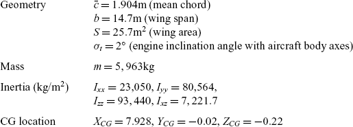
 $6^\circ$ angle-of-attack, Mach 0.25 at an altitude of 2,830m. The mass and geometry of the studied aircraft are given in Table 1. The thrust is computed before parameter estimation and is used in the estimation process as an input variable. With the use of the aircraft state-space model (1) and the observation model (3), the FEM is first applied to the flight data (Reference Jategaonkar and Plaetschke31,Reference Jategaonkar32) to estimate the state noise distribution matrix F in addition to the aerodynamic derivatives and thus calculate the process noise covariance
 $Q = F{F^{ - 1}}{\Delta t ^{ - 1}}$, where
 $\Delta t$ is the sampling time. The estimated true value of Q is
 $diag[0.0012,0.0038,0.0008,0.0075]$.
Geometry and moment of inertia of the aircraft under consideration

We introduce the initial states [ $\beta$, p, r,
 $\phi$] as
 $[ -0.0015 \ \ 0.0197 \ \ 0.0020\ -0.0151]$ and the state propagation error covariance matrix
 $P_0$ =
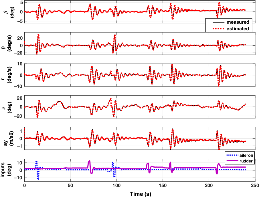
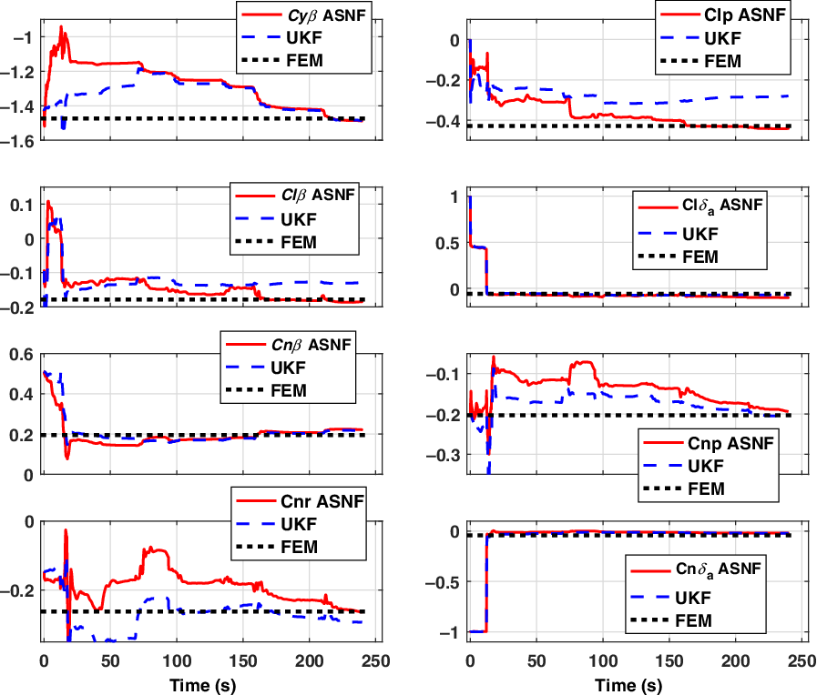
 $diag[0.9 \ \ 1.8 \ \ 1.1 \ \ 3]$ for the application of the proposed ASNF algorithm. Figure 1 shows the flight measured and model estimated response for the small civilian aircraft. The match between the flight measured and model estimated responses is acceptable. A similar parameter estimation procedure is carried out using the UKF with the true values of Q and R, to compare their performance for aerodynamic parameter estimation. Figure 2 shows the performance of the ASNF method for aerodynamic parameter estimation from flight data. It shows that the convergence of the estimates obtained by the ASNF method is similar to the UKF while the difference between their estimated values is marginal and acceptable. The aerodynamic parameters estimated using the ASNF method are much closer to the EEM estimates compared with those obtained using the UKF. The marginal difference in the UKF estimates compared with the ASNF estimates may be due to the usage of a fixed noise covariance of Q and R in the UKF for multiple manoeuvres instead of time-varying Q and R as in the proposed approach of ASNF. Hence, the ASNF method shows appreciable applicability even without knowledge of Q and R.
Flight estimation responses using ASNF method.

Comparison of parameter estimates.

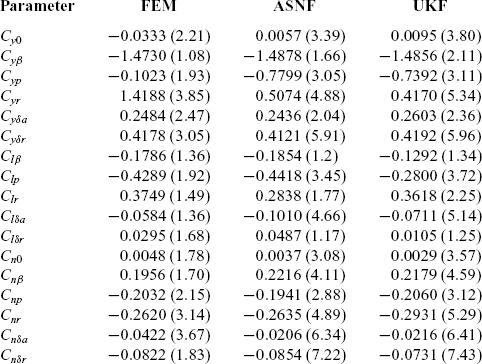
Table 2 compares the numerical values to four decimal places of the estimated lateral directional aerodynamic parameters determined using the different methods. Note that the parameter estimates using all these methods are in close vicinity to one another, and all the numerical values are in good agreement. This accurate mathematical model for the aircraft system under consideration can largely be attributed to the performance of these methods and their close agreement. Here, we highlight the application of ASNF to obtain an aircraft model under variation of both process and measurement noise due to external disturbances.
Estimated lateral directional aerodynamic derivatives

Note: Values in parenthesis denote standard deviation in percentage.
4.1 Dynamic changes of noise covariance matrices
This subsection illustrates the credibility of the proposed approach by testing the estimation accuracy of the ASNF under the situation of varying process and measurement noise covariances. The change of the true values of both the process and measurement noise intensities is assumed to be
 \begin{equation} \left. {\begin{array}{*{20}{l}} {{Q_{T0}} = diag\{ [1.2,3.8,0.8,0.75] \times {{10}^{ - 3}}\} }\\[6pt]
{{R_{T0}} = diag\left\{ {\left[ {8.3 \times {{10}^{ - 3}},0.0317,0.0153,70.45,0.154} \right]} \right\}} \end{array}} \right\}t
< 20{\rm s}\end{equation}
 \begin{equation} \left. {\begin{array}{*{20}{l}} {{Q_T} = diag\{ [1.2,3.8,0.8,0.75] \times {{10}^{ - 7}}\} }\\[6pt]
{{R_T} = diag\left\{ {\left[ {8.3 \times {{10}^{ - 3}},0.0317,0.0153,70.45,0.154} \right] \times {{10}^{ - 2}}} \right\}} \end{array}} \right\}t \ge 20{\rm s}\end{equation}
The prior knowledge of both the process and measurement noise covariance in the UKF are selected as  $Q={Q_{T0}}$ and
 $ R={R_{T0}}$. They are changed after 20s to
 $Q={Q_{T}}$ and
 $ R={R_{T}}$ in (16). However, in the case of ASNF, the initial values of the process and measurement noise intensities are fixed to very small quantities to confirm the possibility of selecting arbitrarily small values of Q and R.
 \begin{equation} \begin{array}{*{20}{l}} {\left. {\begin{array}{*{20}{l}} {Q_{T0}^{asnf} = diag\{ [1.2,3.8,0.8,0.75] \times {{10}^{ - 16}}\} }\\[6pt]
{R_{T0}^{asnf} = diag\left\{ {\left[ {8.3 \times {{10}^{ - 3}},0.0317,0.0153,70.45,0.154} \right] \times {{10}^{ - 10}}} \right\}} \end{array}} \right\}t
< 20{\rm s}}\\[18pt]
{\left. {\begin{array}{*{20}{l}} {Q_T^{asnf} = diag\{ [1.2,3.8,0.8,0.75] \times {{10}^{ - 12}}\} }\\[6pt]
{R_T^{asnf} = diag\left\{ {\left[ {8.3 \times {{10}^{ - 3}},0.0317,0.0153,70.45,0.154} \right] \times {{10}^{ - 12}}} \right\}} \end{array}} \right\}t \ge 20{\rm s}} \end{array}\end{equation}
As a result, Q and R of ASNF are randomly selected with small values  ${Q_{T0}^{asnf}}$ and
 ${R_{T0}^{asnf}}$, respectively, without prior knowledge of the noise statistics. They are changed to
 ${Q_T^{asnf}} $ and
 ${R_T^{asnf}}$ after 20s. Under the same condition of changing noise intensities, the ASNF and UKF methods are applied to estimate the aerodynamic static directional derivative
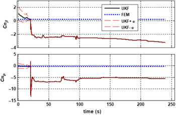
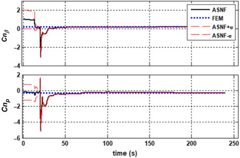
 $Cn\beta$ and cross derivative Cnp influencing the Dutch roll mode. The time history of these derivatives given by UKF and ASNF is shown in Figs 3 and 4, respectively. In UKF, we can see that the estimated parameters diverge after 20s because the prior covariance setting of UKF fails to meet the actual values. Meanwhile, the parameters estimated by ASNF converge to the same as before (Fig. 4), even though the noise covariance matrices have changed.
UKF: divergence of parameter estimates when changing noise covariances.

ASNF: convergence of parameter estimates when changing noise covariances.

In practice, there is the possibility of an error on the order of  $10^{-4}$ in the assumption of the process noise covariance and
 $10^{-2}$ in the measurement noise covariance. This will degrade the performance of the UKF through parameter divergence, as shown in Fig. 3. This major issue is addressed in the ASNF approach by estimating both the process and measurement noise covariances instantly, thus achieving better online estimates of the flight stability and control parameters under varying noise statistics.
5.0 CONCLUSIONS
This paper describes an estimation procedure for lateral directional aerodynamic parameters from flight data in the presence of unknown noise characteristics. The proposed adaptive stochastic non-linear filter (ASNF) method is an efficient technique to obtain the aerodynamic stability and control parameters for an aircraft in an uncertain environment where the noise characteristics change drastically. The investigations are carried out on flight data containing multiple manoeuvres of a small transport aircraft undergoing lateral directional motion. Subsequently, the performance of the ASNF is demonstrated for identifying the aircraft system dynamics from flight test data, being superior to the UKF in terms of fast convergence and estimation accuracy when changing the noise statistics. Therefore, the potential use of ASNF is favourable for the design of adaptive flight controllers for recursive estimation of unobserved states in an aircraft system model and unknown aerodynamic parameters. The efficacy of the proposed approach is significant since the presence of process noise complicates parameter estimation severely as it is non-measurable.
SUPPLEMENTARY MATERIAL
To view supplementary material for this article, please visit https://doi.org/10.1017/aer.2021.61