Introduction
Several methods have been developed to model electromagnetic wave propagation in non-concentric multilayered cylindrical waveguides for a range of applications. One approach, utilizing the method of separation of variables in a bipolar coordinate system, has been used to determine cutoff frequencies for isotropic media waveguides in several configurations, including eccentric coaxial waveguides [Reference Gholizadeh, Baharian and Kashani1], circular waveguides loaded with eccentric rods [Reference Gholizadeh and Hojjat Kashani2], and eccentric two-layer coaxial waveguides [Reference Gholizadeh and Hojjat Kashani3]. Perturbation methods have also been utilized to calculate axial wavenumbers and field patterns for uniaxially anisotropic media waveguides, particularly in eccentric coaxial waveguides and circular waveguides with eccentric rods [Reference Gonçalves, Rosa and Teixeira4, Reference Gonçalves, Rosa and Teixeira5]. Additionally, a hybrid method combining perturbation techniques with transformation optics (TO) has been applied to model the waveguide problem comprised by electromagnetic logging sensors in eccentric subsurface boreholes [Reference Rosa, Bergmann, Teixeira and Novo6]. Furthermore, Graf’s addition theorem for cylindrical functions has been used to model Gaussian beam scattering by a circular perfect electric conductor (PEC) coated with eccentric anisotropic media [Reference Mao, Wu, Zhang, Gao and Yang7], as well as for well-logging sensors in multicentric cylindrically layered earth formations [Reference Liu, Teixeira and Zhang8].
The spectral element method (SEM) is a versatile technique for the analysis of electromagnetic fields that have demonstrated effectiveness in various applications [Reference Liu, Cai, Zhu, Tang and Liu9–Reference Ribeiro, Rosa, Bergmann and Teixeira14]. A preliminary study [Reference Ribeiro, Rosa and Bergmann11] shows that an SEM-based technique in cylindrical coordinates is more efficient than the conventional Cartesian approach [Reference Liu, Cai, Zhu, Tang and Liu9] for modeling cylindrical-conforming boundaries, as it requires fewer elements and degrees of freedom (DoFs). The study provided in [Reference Ribeiro, Rosa and Bergmann11] improves upon previous work [Reference Liu, Cai, Zhu, Tang and Liu9, Reference Liu, Jiang, Liu and Liu10] by representing fields and medium tensors directly in cylindrical coordinates. In [Reference Ribeiro, Gonçalves, Rosa, Bergmann and Teixeira13, Reference Ribeiro, Rosa, Bergmann and Teixeira14], SEM was used to model both an eccentric coaxial waveguide and a circular waveguide loaded with an eccentric rod filled with uniaxially anisotropic media. Notably, this formulation employs TO to map the eccentric problem to a concentric one, allowing SEM to solve the transformed domain. Unlike perturbation-based techniques, this approach is not limited to problems with small eccentricities [Reference Gonçalves, Rosa and Teixeira4–Reference Rosa, Bergmann, Teixeira and Novo6].
In the present work, we extend previous TO studies [Reference Rosa, Bergmann, Teixeira and Novo6, Reference Ribeiro, Gonçalves, Rosa, Bergmann and Teixeira13], which were restricted to uniaxially anisotropic tensors, to include general anisotropic non-reciprocal media characterized by non-symmetric and non-Hermitian tensors. We then apply the cylindrical SEM to model these transformed problems. Additionally, we extend the earlier formulation from [Reference Ribeiro, Rosa, Bergmann and Teixeira15], which was limited to radially bounded eccentric two-layer waveguides, to model non-concentric multilayered waveguides and radially unbounded problems. This is achieved using a complex-stretched perfectly matched layer (PML) to simulate open boundary conditions.
Eccentric waveguide problem
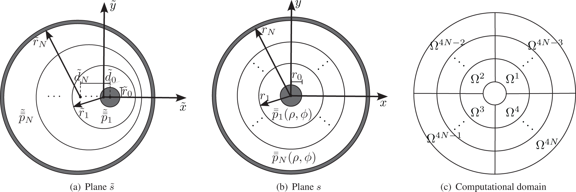
Consider a non-concentric multilayered waveguide invariant along the axial direction, as depicted in Fig. 1(a). The eccentric geometry is represented in a cylindrical coordinate system denoted by  $(\tilde{\rho},\tilde{\phi},\tilde{z})$. The geometry is defined in terms of three circular interfaces associated with the radii
 $\tilde{r}_0$,
 $\tilde{r}_1$,
 $\ldots$,
 $\tilde{r}_N$. Additionally, said cylinders are offset with respect to the
 $\tilde{z}$-axis by the distances
 $\tilde{d}_0$,
 $\tilde{d}_1$,
 $\ldots$, and
 $\tilde{d}_N$. Positive offsets are defined as those that move the boundaries toward the positive
 $\tilde{x}$ direction. The waveguide is radially bounded by a PEC at the
 $\tilde{r}_0$ and
 $\tilde{r}_N$ boundaries. We assume a time-harmonic dependence of the form
 $e^{-i \omega t}$. The media are characterized by the real-valued permeability tensor
 \begin{equation}
\tilde{\bar{\bar{\mu}}}_j =\mu_0 \tilde{\bar{\bar{\mu}}}_{r,j},
\end{equation}
(a) Geometry of an eccentric multilayered coaxial waveguide. (b) Geometry of the mapped concentric multilayered coaxial waveguide. (c) Equivalent computational domain partitioned into curvilinear elements.

with
 \begin{equation}
\tilde{\bar{\bar{\mu}}}_{r,j}=
\begin{bmatrix}
\tilde{\mu}_{\rho \rho,j} & \tilde{\mu}_{\rho \phi,j} & 0\\
\tilde{\mu}_{\phi \rho,j} & \tilde{\mu}_{\phi \phi,j} & 0\\
0 & 0 & \tilde{\mu}_{z,j}
\end{bmatrix},
\end{equation}
and the complex-valued permittivity tensor
 \begin{equation}
\tilde{\bar{\bar{\epsilon}}}_{j} = \epsilon_0 \tilde{\bar{\bar{\epsilon}}}_{c,j} = \epsilon_0 \left( \tilde{\bar{\bar{\epsilon}}}_{r,j} + \frac{i}{\omega \epsilon_0} \tilde{\bar{\bar{\sigma }}}_j \right),
\end{equation}
with
 \begin{equation}
\tilde{\bar{\bar{\epsilon}}}_{r,j}=
\begin{bmatrix}
\tilde{\epsilon}_{\rho \rho,j} & \tilde{\epsilon}_{\rho \phi,j} & 0\\
\tilde{\epsilon}_{\phi \rho,j} & \tilde{\epsilon}_{\phi \phi,j} & 0\\
0 & 0 & \tilde{\epsilon}_{z,j}
\end{bmatrix},
\end{equation}
and
 \begin{equation}
\tilde{\bar{\bar{\sigma}}}_j=
\begin{bmatrix}
\tilde{\sigma}_{\rho \rho,j} & \tilde{\sigma}_{\rho \phi,j} & 0\\
\tilde{\sigma}_{\phi \rho,j} & \tilde{\sigma}_{\phi \phi,j} & 0\\
0 & 0 & \tilde{\sigma}_{z,j}
\end{bmatrix},
\end{equation}
expressed in cylindrical coordinates  $(\tilde{\rho},\tilde{\phi},\tilde{z})$, where
 $j=1,2,\ldots,N$ representing each layer.
Transformation optics
From conformal TO [Reference Rosa, Bergmann, Teixeira and Novo6, Reference Teixeira and Chew16, Reference Xu and Chen17], we can transform the eccentric problem into an equivalent concentric problem (represented in Fig. 1(b)) using analytic functions in the complex plane. The eccentric plane can be written by  $\tilde{s}=\tilde{x}+i\tilde{y}$ and the concentric plane by
 $s=~x+iy$. In addition, let
 $z=\tilde{z}$, we can map the two planes via
 \begin{equation}
s= \tilde{x}_2 \frac{\tilde{s}-\tilde{x}_1}{\tilde{s}-\tilde{x}_2},
\end{equation}
where
 \begin{equation}
\tilde{x}_{1,2}=\frac{-\tilde{c} \mp \sqrt{\tilde{c}^2-4 \tilde{r}_j^2}}{2}, \;\;\; \tilde{c}=\frac{\tilde{r}_0^2-\tilde{r}_j^2-\tilde{d}_0^2}{\tilde{d}_0},
\end{equation}
and  $\tilde{r}_j$ represent the concentric interface in plane
 $\tilde{s}$. The mapping in (6) satisfies Cauchy–Riemann conditions [Reference Xu and Chen17]
 \begin{equation}
\frac{\partial x}{\partial \tilde{x}} = \frac{\partial y}{\partial \tilde{y}}, \;\;\;\; \frac{\partial x}{\partial \tilde{y}} = -\frac{\partial y}{\partial \tilde{x}}.
\end{equation}
The original electromagnetic problem in the eccentric coordinates  $(\tilde{\rho},\tilde{\phi},\tilde{z})$ can be transformed into a concentric problem with coordinates
 $(\rho,\phi,z)$ using the field transformation
 \begin{equation}
\mathbf{F}=\bar{\bar{J}}_{\mathrm{TO}} \cdot \tilde{\mathbf{F}}, \;\; \text{with} \;\; \mathbf{F} \in \{\mathbf{E},\mathbf{H} \},
\end{equation}
 \begin{equation}
\bar{\bar{p}}=|\bar{\bar{J}}_{\mathrm{TO}}|^{-1} \bar{\bar{J}}_{\mathrm{TO}} \cdot \tilde{\bar{\bar{p}}} \cdot \bar{\bar{J}}_{\mathrm{TO}}^T, \;\; \text{with} \;\; p \in \{\mu,\epsilon \} ,
\end{equation}
where  $\bar{\bar{J}}_{\mathrm{TO}}$ is the Jacobian of the transformation
 $(\tilde{\rho},\tilde{\phi},\tilde{z}) \rightarrow (\rho,\phi,z)$, and
 $|\bar{\bar{J}}_{\mathrm{TO}}|$ is the respectively determinant. The Jacobian matrix
 $\bar{\bar{J}}_{\mathrm{TO}}$ is expressed as
 \begin{equation}
\bar{\bar{J}}_{\mathrm{TO}}= \bar{\bar{R}} (\phi) \cdot \bar{\bar{J}}_{xyz} \cdot \bar{\bar{R}}^T (\tilde{\phi}),
\end{equation}
in which  $\bar{\bar{J}}_{xyz}$ is the Jacobian associated with the transformation
 $(\tilde{x},\tilde{y},\tilde{z}) \rightarrow (x,y,z)$, and
 $\bar{\bar{R}}(\phi)$ is the transformation matrix for Cartesian-to-cylindrical components. Using the condition (8), we obtain
 \begin{equation}
\bar{\bar{J}}_{xyz}=
\begin{bmatrix}
\dfrac{\partial x}{\partial \tilde{x}} & \dfrac{\partial x}{\partial \tilde{y}} & 0\\
-\dfrac{\partial x}{\partial \tilde{y}} & \dfrac{\partial x}{\partial \tilde{x}} & 0\\
0 & 0 & 1
\end{bmatrix},
\;\bar{\bar{R}}(\phi)=
\begin{bmatrix}
\cos \phi & \sin \phi & 0\\
-\sin \phi & \cos \phi & 0\\
0 & 0 & 1
\end{bmatrix},
\end{equation}
where
 \begin{align}
\frac{\partial x}{\partial \tilde{x}} &= \big[ (\tilde{x}-\tilde{x}_2)^2 -\tilde{y}^2 \big] \frac{\tilde{x}_2(\tilde{x}_1-\tilde{x}_2)}{\big[ (\tilde{x}-\tilde{x}_2)^2 +\tilde{y}^2 \big]^2},
\end{align}
 \begin{align}
\frac{\partial x}{\partial \tilde{y}} &= 2\tilde{y}(\tilde{x}-\tilde{x}_2) \frac{\tilde{x}_2(\tilde{x}_1-\tilde{x}_2)}{\big[ (\tilde{x}-\tilde{x}_2)^2 +\tilde{y}^2 \big]^2}.
\end{align}
Based on the approach developed in [Reference Liu, Cai, Zhu, Tang and Liu9, Reference Vardapetyan and Demkowicz18–Reference Ribeiro20], we define a variational waveguide problem for the concentric cylindrical cross-section Ω (illustrated in Fig. 1(b)). Now, we wish to determine all pairs  $(k_z,(\mathbf{e}_s,e_z)) \in (\mathbb{C}, \mathbf{H}_0 (\text{curl}, \Omega)~\times~H_0^1 (\Omega))$ that satisfy
 \begin{equation}
\left\{
\begin{array}{rr}
\langle \mu_{zz}^{-1} \boldsymbol{\nabla}_s \times \mathbf{e}_s, \boldsymbol{\nabla}_s \times \mathbf{w} \rangle +i k_z \langle \bar{\bar{\mu}}_{s}^{-1} \boldsymbol{\nabla}_s e_z , \mathbf{w} \rangle
\\
-k_0^2 \langle \bar{\bar{\epsilon}}_{cs} \mathbf{e}_s, \mathbf{w} \rangle + k_z^2 \langle \bar{\bar{\mu}}_{s}^{-1} \mathbf{e}_s, \mathbf{w} \rangle = 0
\\[1em]
\langle \bar{\bar{\epsilon}}_{cs} \mathbf{e}_s , \boldsymbol{\nabla}_s w \rangle -i k_z \langle \epsilon_{cz} e_z, w \rangle = 0
\end{array}
\right.
\end{equation}
for all  $(\mathbf{w},w) \in \mathbf{H}_0 (\text{curl}, \Omega) \times H_0^1 (\Omega)$. In the above,
 $\mathbf{e}_s = (e_\rho, e_\phi)^T$ and ez are the transversal and axial electric field components, and kz is the associated axial wavenumber. The transverse Laplacian operator is
 $\boldsymbol{\nabla}_s= ( {\partial}/{\partial \rho} , {\rho}^{-1} {\partial}/{\partial \phi} )^T$, and the transverse and axial components of the relative permeability and permittivity tensors are given by
 $\bar{\bar{\mu}}_{s}$,
 $\bar{\bar{\epsilon}}_{cs}$ and µz, ϵcz, respectively. In addition, the notation
 $\langle\cdot, \cdot \rangle$ represents an inner product (for both scalar and vector functions),
 $\mathbf{H}_0 (\text{curl}, \Omega)$ and
 $H_0^1 (\Omega)$ are the Hilbert spaces, as defined in [Reference Ribeiro20, Sec. 2.2]. The domain is truncated by a PEC, so the boundary conditions to be imposed on the boundary of the domain (at
 $\rho=r_0$ and
 $\rho=r_N$) are
 \begin{equation}
\left.
\begin{array}{rr}
\mathbf{e}_s \times \hat{n} &= \mathbf{0} \\
e_z &=0
\end{array}
\right. \;\;\; \text{on} \; \partial \Omega,
\end{equation}
where  $\hat{n}$ is the outward unit normal vector on the boundary of the domain
 $\partial \Omega$.
Higher-order SEM
The SEM is a higher-order implementation of the finite element method (FEM), which also involves discretizing the computational domain into elements. However, unlike FEM, SEM employs specific orthogonal polynomial families to determine the location of internal nodes within each element. This approach enables SEM to achieve spectral convergence, where the error decreases exponentially with increasing polynomial order.
Computational domain
The cross-section Ω of the concentric multilayered problem is first discretized into curvilinear elements  $\Omega^e$ for
 $e=~1,2,\ldots,4N$, where N is the number of layers, as shown in Fig. 1(c). Each element is described by the polar coordinates
 $(\rho^e, \phi^e)$, which is then mapped into the reference (Cartesian) coordinates
 $(\xi, \eta)$ via
 \begin{equation}
\rho^{e}(\xi)=0.5(\rho_0^{e}+\rho_1^{e})+0.5(\rho_1^{e}-\rho_0^{e})\xi,
\end{equation}
 \begin{equation}
\phi^{e}(\eta)=0.5(\phi_0^{e}+\phi_1^{e})+0.5(\phi_1^{e}-\phi_0^{e})\eta,
\end{equation}
where  $\xi \in [-1,1]$ and
 $\eta \in [-1,1]$. The superscript e indicates the parameters of the reference square element. Figs. 2 and 3 illustrate the considered mapping. The Jacobian matrix associated with this coordinate transformation is given by
 \begin{align}
\bar{\bar{J}}_s^{e} &= \left[
\begin{array}{cc}
\dfrac{\partial \rho^{e}}{\partial \xi} & \dfrac{\partial \rho^{e}}{\partial \eta}\\
~ \rho^e \dfrac{\partial \phi^{e}}{\partial \xi} & \rho^e \dfrac{\partial \phi^{e}}{\partial \eta}
\end{array}
\right]
\end{align}
 \begin{align*}
&=
\left[
\begin{array}{cc}
0.5(\rho_1^{e}-\rho_0^{e}) & 0 \\
~
0 & 0.5\rho^e (\phi_1^{e}-\phi_0^{e})
\end{array}
\right] .
\end{align*}
Because the above transformation matrix is diagonal, the ρ- and η-directions are decoupled, as well as ϕ- and ξ-directions [Reference Ribeiro, Rosa and Bergmann11–Reference Ribeiro, Gonçalves, Rosa, Bergmann and Teixeira13].
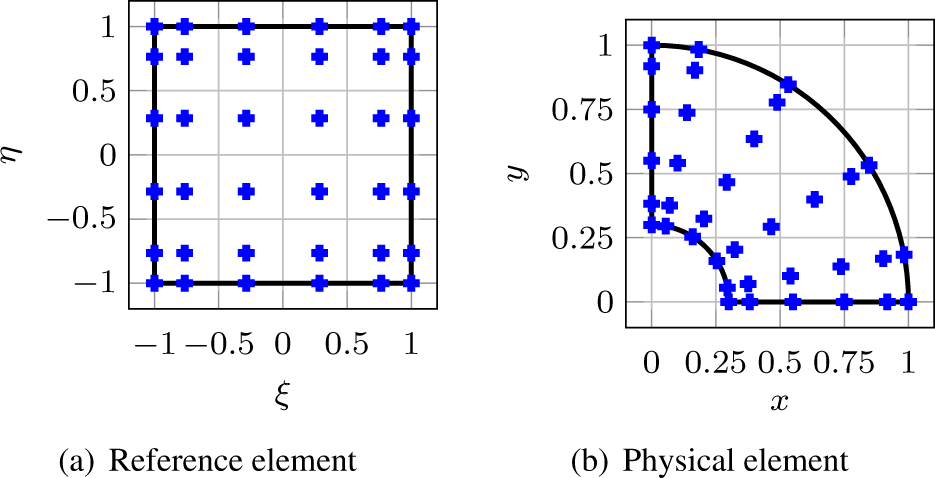
GLL node distributions using expansion order N = 5.

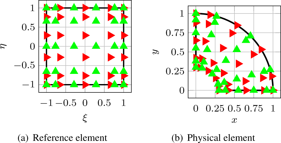
Curl-conforming node distributions using expansion order N = 5.

Lagrange interpolation
The field components in each curvilinear element  $\Omega^e$ are represented using Lagrange interpolation based on Gauss–Lobatto–Legendre (GLL) sampling points. The one-dimensional Nth-order GLL basis function defined in the reference coordinate system is given by
 \begin{equation}
\phi_j^{N} (\xi) = \prod_{k \neq j}^{N+1} \frac{\xi-\xi_k}{\xi_j-\xi_k} \;\; \forall~ \xi \in [-1,1],
\end{equation}
where  $j=1,2,\ldots,N+1$, and N + 1 interpolation nodes ξk correspond to the roots of the
 $(N+1)$-degree completed Lobatto polynomial. The two-dimensional GLL basis function is derived through tensor-product expansions
 \begin{equation}
\hat{\psi}_{z,ij} (\xi,\eta) = \phi_i^{N} (\xi) \phi_j^{N} (\eta) \;\; \forall~ (\xi,\eta) \in [-1,1]^2,
\end{equation}
and the mixed-order curl-conforming vector edge-based basis functions are written as
 \begin{equation}
\begin{array}{c}
\hat{\Phi}_{\xi,ij} (\xi,\eta) = \phi_i^{N-1} (\xi) \phi_j^{N} (\eta)
\\ \\
\hat{\Phi}_{\eta,ij} (\xi,\eta) = \phi_i^{N} (\xi) \phi_j^{N-1} (\eta)
\end{array}
\end{equation}
for all  $(\xi,\eta) \in [-1,1]^2$. As an illustrative example, the GLL node distributions in the reference and physical elements considering expansion function order N = 5 are depicted in Fig. 2. Additionally, the curl-conforming node distributions with the same expansion order are represented in Fig. 3. Note that the node distributions are denser toward the edges of the element, a characteristic that effectively mitigates the occurrence of the Runge effect when employing higher-order expansions [Reference Pozrikidis21].
Generalized eigenvalue problem
To formulate the discrete version of the problem presented in (15), we approximate the transversal electrical components in the reference domain  $\hat{\mathbf{e}}_{s}=(\hat{e}_{\xi},\hat{e}_{\eta})$ using expansions based on vector edge-based basis functions
 \begin{equation}
\hat{e}_{\xi} (\xi,\eta)= \sum_{j=1}^{N(N+1)} \hat{e}_{\xi,j} \hat{\Phi}_{\xi,j} (\xi,\eta),
\end{equation}
 \begin{equation}
\hat{e}_{\eta} (\xi,\eta)= \sum_{j=1}^{N(N+1)} \hat{e}_{\eta,j} \hat{\Phi}_{\eta,j} (\xi,\eta),
\end{equation}
and the axial field  $\hat{e}_{z}$ based on GLL basis functions
 \begin{align}
\hat{e}_{z} (\xi,\eta)= \sum_{j=1}^{(N+1)^2} \hat{e}_{z,j} \hat{\psi}_{z,j} (\xi,\eta).
\end{align}
By using the above expansions and applying the Galerkin method in the variational formulation (15), we obtain the following generalized eigenvalue problem
 \begin{equation}
\left( -\mathbf{S}_{ss}-\mathbf{K}_{sz} \mathbf{M}_{zz}^{-1} \mathbf{K}_{zs} +k_0^2 \mathbf{M}_{ss1} \right) \hat{\mathbf{e}}_{s} = k_z^2 \mathbf{M}_{ss2} \hat{\mathbf{e}}_{s},
\end{equation}
where  $k_z^2$ are the eigenvalues associated with the axial wavenumbers, and
 $\hat{\mathbf{e}}_{s}$ are the eigenvectors associated with the transversal electric field components. The matrices used in (23) have the same basic structure as those found in [Reference Ribeiro20, Sec. 2.3].
Perfectly matched layer
Modeling field propagation in radially unbounded waveguides, such as dielectric rods, optical fibers, and subsurface boreholes, requires appropriate absorbing boundary conditions to mimic open space effectively. In our formulation, we incorporated the complex-stretched PML in cylindrical coordinates [Reference Teixeira and Chew22, Reference Teixeira and Chew23] into the SEM technique. First, we define a one-to-one mapping of the radial coordinate ρ to a complex coordinate  $\tilde{\rho}$ as
 \begin{equation}
\rho \longrightarrow \tilde{\rho}= \int_{0}^{\rho} s_\rho (\rho') \, d\rho'.
\end{equation}
Then, using an integral ensures that  $\tilde{\rho}$ varies smoothly, even if sρ has discontinuities. The complex-stretching function sρ employs a polynomial profile defined in [Reference Rosa24, Sec. 3.3] and expressed as
 \begin{equation}
s_\rho (\rho) = \left\{
\begin{array}{cl}
1, & \rho \in [0,r_{N-1})
\\
1 +i \alpha_\mathrm{PML} \left( \dfrac{\rho - r_{N-1}}{r_{N}-r_{N-1}} \right)^q, & \rho \in [r_{N-1},r_{N}]
\end{array}
\right.
\end{equation}
which yields
 \begin{equation}
\tilde{\rho} = \left\{
\begin{array}{cl}
\rho, & \rho \in [0,r_{N-1})
\\
\rho +i \alpha_\mathrm{PML} \frac{1}{1+q} \dfrac{(\rho-r_{N-1})^{q+1}}{(r_{N}-r_{N-1})^q}, & \rho \in [r_{N-1},r_{N}]
\end{array}
\right.
\end{equation}
where  $q \in \mathbb{N}_0$, and
 $\alpha_\mathrm{PML} \gt 0$.
In the PML region (non-physical domain), the complex-stretched radial coordinate incorporates an imaginary component that represents radial wave attenuation. This function’s smoothness minimizes reflections back into the physical domain, effectively simulating a radial-unbounded space. Please, see [Reference Rosa24–Reference Teixeira and Chew27] for further details.
Numerical results
This section presents numerical examples involving non-concentric multilayered waveguide problems using the proposed SEM formulation. First, we analyze eccentric two-layer waveguides filled with anisotropic reciprocal and non-reciprocal media over a wide frequency range. Second, we apply the formulation to model three-layer waveguides. Finally, we employ the formulation to address radially unbounded problems using a complex-stretched PML. To validate our formulation, we compare the SEM results with those obtained from FEM from COMSOL Multiphysics [28]. Our SEM codes were implemented in MATLAB [29]. Both methods run on a 1.80-GHz Intel Core i7 processor PC with four cores.
Eccentric two-layer waveguides
As our first validation, we consider the problem characterized by the radii  $\tilde{r}_0=1\,\mathrm{mm}$,
 $\tilde{r}_1=5.36\,\mathrm{mm}$,
 $\tilde{r}_2=10\,\mathrm{mm}$, and offsets
 $\tilde{d}_0=2\,\mathrm{mm}$,
 $\tilde{d}_1=1.42\,\mathrm{mm}$,
 $\tilde{d}_2=0\,\mathrm{mm}$. The media are described by the relative permittivity and electrical conductivity diagonal tensors represented in cylindrical coordinates by
 \begin{equation}
\tilde{\bar{\bar{\epsilon}}}_{r,1}=
\begin{bmatrix}
5.7 & 0 & 0\\
0 & 2.3 & 0\\
0 & 0 & 4.1
\end{bmatrix}, \;\;
\tilde{\bar{\bar{\sigma}}}_1=
\begin{bmatrix}
0.38 & 0 & 0\\
0 & 0.25 & 0\\
0 & 0 & 0.30
\end{bmatrix},
\end{equation}
 \begin{equation}
\tilde{\bar{\bar{\epsilon}}}_{r,2}=
\begin{bmatrix}
4.3 & 0 & 0\\
0 & 2.7 & 0\\
0 & 0 & 3.9
\end{bmatrix}, \;\;
\tilde{\bar{\bar{\sigma}}}_2=
\begin{bmatrix}
0.14 & 0 & 0\\
0 & 0.21 & 0\\
0 & 0 & 0.23
\end{bmatrix}.
\end{equation}
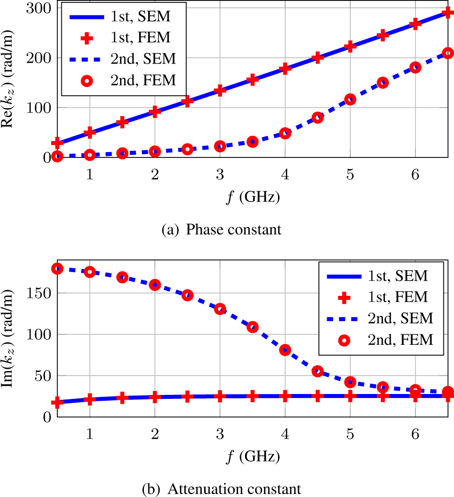
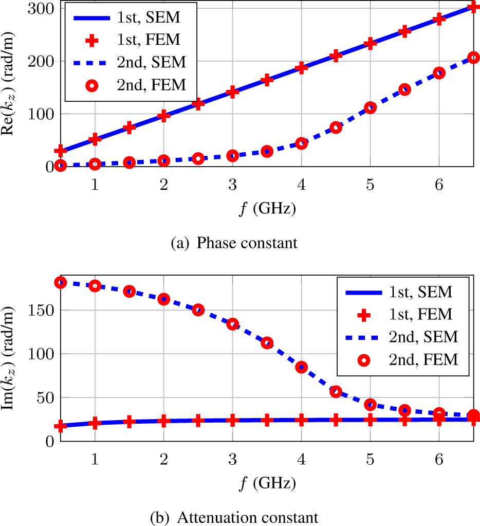
The permeability parameter is that of the vacuum. Figure 4 shows the real and imaginary part of axial wavenumber kz for the first two hybrid modes as a function of the operating frequency f varying from  $0.5\,\mathrm{GHz}$ to
 $6.5\,\mathrm{GHz}$. The results obtained with the proposed SEM show excellent agreement with those from the FEM.
Axial wavenumbers for the first two modes in an eccentric anisotropic two-layer waveguide considering offset  $\tilde{d}_2=0$.

As a second example, we investigate a similar problem, but now there is a negative offset  $\tilde{d}_2$. The geometry parameters are defined by
 $\tilde{r}_0=1\,\mathrm{mm}$,
 $\tilde{r}_1=5\,\mathrm{mm}$,
 $\tilde{r}_2=9.96\,\mathrm{mm}$,
 $\tilde{d}_0=1\,\mathrm{mm}$,
 $\tilde{d}_1=0\,\mathrm{mm}$, and
 $\tilde{d}_2=-2.68\,\mathrm{mm}$. We consider the waveguide filled with the same media as before. Figure 5 shows the results for the first two hybrid modes as a function of frequency. Again, we obtained excellent agreement between the SEM and FEM solutions.
Axial wavenumbers for the first two modes in an eccentric anisotropic two-layer waveguide considering offset  $\tilde{d}_1=0$.

Now, we will explore the capabilities of the present SEM formulation to model waveguides that operate in low-frequency and are filled with more complex anisotropic materials, where the media are non-reciprocal and described by non-symmetric and non-Hermitian tensors. This scenario is particularly relevant for well-logging tools used in geophysical exploration. Consider the scenario defined by the radii  $\tilde{r}_0=4\,\mathrm{in}$,
 $\tilde{r}_1=10\,\mathrm{in}$,
 $\tilde{r}_2=16.32\,\mathrm{in}$, and the eccentricity offsets
 $\tilde{d}_0=1\,\mathrm{in}$,
 $\tilde{d}_1=0\,\mathrm{in}$,
 $\tilde{d}_2=-1.91$ in, where
 $1\,\mathrm{in}=2.54\times 10^{-2}\,\mathrm{m}$. The relative permittivity and electrical conductivity tensors are given by
 \begin{equation}
\tilde{\bar{\bar{\epsilon}}}_{r,1}=
\begin{bmatrix}
1.9 & 2.3 & 0\\
2.7 & 1.8 & 0\\
0 & 0 & 2.8
\end{bmatrix}, \;\;
\tilde{\bar{\bar{\sigma}}}_1= 10^{-4}
\begin{bmatrix}
5 & 4 & 0\\
3 & 2 & 0\\
0 & 0 & 6
\end{bmatrix},
\end{equation}
 \begin{equation}
\tilde{\bar{\bar{\epsilon}}}_{r,2}=
\begin{bmatrix}
3.7 & 4.3 & 0\\
4.2 & 3.0 & 0\\
0 & 0 & 3.2
\end{bmatrix}, \;\;
\tilde{\bar{\bar{\sigma}}}_2= 10^{-2}
\begin{bmatrix}
4 & 5 & 0\\
2 & 3 & 0\\
0 & 0 & 5
\end{bmatrix}.
\end{equation}
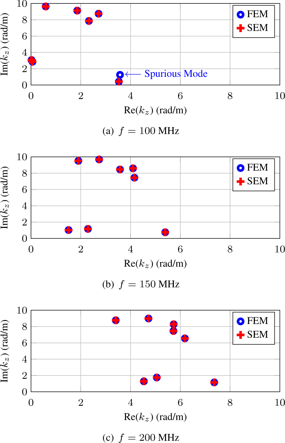
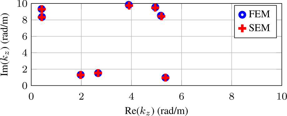
The permeability is once again the same as that of the vacuum. Assuming frequencies  $f \in \{100,150,200\}\,\mathrm{MHz}$, the results for the axial wavenumbers kz from our formulation are compared with FEM results in the complex region
 $[0,10]^2$. Excellent agreement is observed in Fig. 6. For the case
 $f=100\,\mathrm{MHz}$, the FEM solution presented one spurious mode, which can be seen in Fig. 6(a). Such eigenvalue is located near the least attenuated mode, and its non-physical characteristics were confirmed by inspecting the field distribution, which exhibits a highly irregular spatial distribution.
Axial wavenumbers obtained over the complex region  $[0,10]^2$ for non-concentric two-layer waveguides filled with anisotropic non-reciprocal media.

In the three examples examined here, the SEM computational domains were discretized into 8 elements with expansion functions of order 7, resulting in 676 DoF and a computational time of 36 seconds. For the FEM model, a cubic-order discretization with a finer physics-controlled mesh option was utilized to obtain reference solutions, leading to 11484 DoF for the first example, 11880 DoF for the second, and 10920 DoF for the third. The computational time for COMSOL was approximately 40 seconds. Notably, the current SEM formulation requires roughly 6% of the DoFs compared to the FEM model while maintaining a similar computational time.
Eccentric three-layer waveguides
We now consider an eccentric three-layer waveguide. The waveguide is truncated by PEC at  $\tilde{r}_0=4$ in and
 $\tilde{r}_3=23.17$ in, with the non-concentric interfaces defined by the radii
 $\tilde{r}_1=10\,\mathrm{in}$,
 $\tilde{r}_2=16.32\,\mathrm{in}$. The eccentricity offsets are given by
 $\tilde{d}_0=1\,\mathrm{in}$,
 $\tilde{d}_1=0\,\mathrm{in}$,
 $\tilde{d}_2=-1.91\,\mathrm{in}$,
 $\tilde{d}_3=-4.87\,\mathrm{in}$. The material parameters for the first two layers are the same as in the previous example, with permittivity defined in (28a) and (28b). The third layer is characterized by a material with non-symmetric and non-Hermitian tensors
 \begin{equation}
\tilde{\bar{\bar{\epsilon}}}_{r,3}=
\begin{bmatrix}
6.1 & 5.4 & 0\\
4.3 & 7.2 & 0\\
0 & 0 & 5.9
\end{bmatrix}, \;\;
\tilde{\bar{\bar{\sigma}}}_3= 10^{-1}
\begin{bmatrix}
7 & 3 & 0\\
4 & 5 & 0\\
0 & 0 & 8
\end{bmatrix}.
\end{equation}
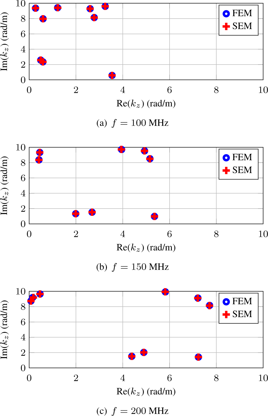
The unstated parameters are assumed to be the same as those of vacuum. For the frequencies  $f \in\{100,150,200\}$ MHz, we compared the axial wavenumber results from our formulation with those obtained using FEM in the complex domain
 $[0,10]^2$ for the three-layer waveguide case. As shown in Fig. 7, the results demonstrate excellent agreement.
Axial wavenumbers obtained over the complex region  $[0,10]^2$ for non-concentric three-layer waveguides filled with anisotropic non-reciprocal media.

The SEM model used an expansion order of N = 7 and the domain was discretized into 12 elements, demanding a computational time of 45 seconds and 1012 DoFs. In contrast, the FEM model, employing cubic-order discretization and a finer physics-controlled mesh, resulted in 12420 DoFs and a computational time of 50 seconds. The SEM requires approximately 8% of the DoFs used in the FEM model and achieves comparable accuracy with a similar computation time.
Radially unbounded waveguides
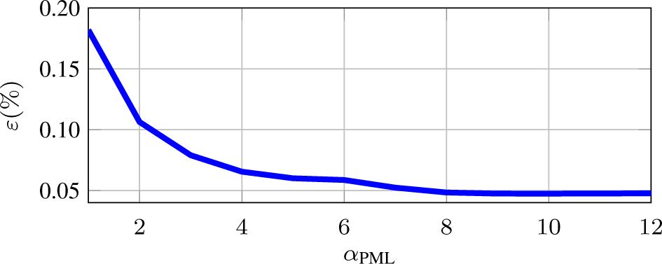
Finally, we investigate the radially unbounded problem. As a validation case, we consider the same eccentric three-layer waveguides as before, but now without the external PEC truncation. We set the polynomial order q = 0 in (25) to obtain the linear complex radial coordinate in (26). For a fixed frequency of 150 MHz, we examine the SEM convergence behavior as a function of the PML parameter  $\alpha_{\text{PML}}$, using FEM as a reference solution, as depicted in Fig. 8. The relative percentage error is approximately
 $0.05\%$ from
 $\alpha_{\text{PML}} = 8$. Considering
 $\alpha_{\text{PML}} = 10$, we plot the axial wavenumber over the complex region
 $[0, 10]^2$ for a fixed frequency
 $f = 150\,\mathrm{MHz}$ in Fig. 9. Once again, we note excellent agreement between the SEM and FEM solutions.
Relative percentage error of the first mode as a function of the PML parameter  $\alpha_{\text{PML}}$ operating in
 $150\,\mathrm{MHz}$.

Axial wavenumbers obtained over the complex region  $[0,10]^2$ for radially unbounded eccentric three-layer waveguide filled with anisotropic non-reciprocal media operating in
 $150\,\mathrm{MHz}$ and using
 $\alpha_{\text{PML}}=10$.

Regarding the computational cost, the SEM model with an expansion order of N = 7 and discretized into 16 elements (including 4 elements for the PML region) results in 1348 DoFs. The FEM model, employing cubic-order discretization and a finer physics-controlled mesh in COMSOL, results in 14712 DoFs. The SEM requires approximately 9% of the DoFs of the FEM. Both methods have a computational time of about 60 seconds.
Conclusion
This study presented a higher-order SEM designed to analyze eccentric multilayered waveguides filled with anisotropic reciprocal and non-reciprocal media. By applying conformal TO, we simplified the eccentric waveguide geometry into a more manageable concentric one. We employed higher-order two-dimensional basis functions based on the zeros of the completed Lobatto polynomial to represent the fields in the concentric domain. To simulate the radially unbounded domain, we incorporated a complex-stretched PML into our formulation. Our method demonstrated both accuracy and efficiency in modeling lossy and anisotropic waveguides across a broad frequency spectrum. Future research will extend this SEM formulation to include driven problems with antenna excitations, allowing for the simulation of additional problems such as logging-while-drilling sensors in eccentric subsurface boreholes with invasion zones. This capability is of significant importance for geophysical exploration applications.
Funding statement
This work was supported in part by the São Paulo Research Foundation (FAPESP), Brazil, under Grant 2024/05690-0.
Competing interests
The authors report no conflict of interest.

Raul O. Ribeiro received the B.S. degree in electrical engineering from the Federal University of Pampa, Alegrete, Brazil, in 2017, the M.S. degree in applied mathematics from the Federal University of Rio Grande do Sul, Porto Alegre, Brazil, in 2019, and the Ph.D. degree in electrical engineering from the Pontifical Catholic University of Rio de Janeiro, Rio de Janeiro, Brazil, in 2024. He was a Graduate Research Visitor at the ElectroScience Laboratory, The Ohio State University, USA, in 2023. He is currently a Postdoc Researcher at the School of Engineering, UNESP, São João da Boa Vista, SP, Brazil. His current research interest includes numerical methods in electromagnetics and wave propagation modeling in complex media.

Guilherme S. Rosa received the B.S. degree in electrical engineering from the Federal University of Santa Maria, Santa Maria, Brazil, in 2011, and the M.S. and the Ph.D. degrees in electrical engineering from the Pontifical Catholic University of Rio de Janeiro, Rio de Janeiro, Brazil, in 2013 and 2017, respectively. He was a Professor at the Department of Electrical Engineering and Center for Telecommunications Studies at the Pontifical Catholic University of Rio de Janeiro from 2018 to 2024. In 2024, he joined São Paulo State University, São João da Boa Vista, Brazil, as a Professor in the School of Engineering. His current research interests include pseudo-analytical techniques for wave propagation modeling in complex media.

José R. Bergmann received the degree in electrical engineering from Universidade Federal do Rio Grande do Sul, Brazil, in 1975, the M.Sc. degree in electrical engineering from Instituto Militar de Engenharia, Brazil, in 1979, and the Ph.D. degree in electrical engineering from Queen Mary College, University of London, London, U.K., in 1986. He joined the Pontifical Catholic University of Rio de Janeiro (PUC-Rio) in 1979, where he is currently a Professor with the Department of Electrical Engineering. He was Head of the Antenna Group of the Center of Telecommunications Studies (CETUC) and, between 2007 and 2022, he was Vice-President for Academic Affairs of PUC-Rio. His research interests comprise numerical modeling, synthesis, and analysis of reflector systems. Dr. Bergmann was Vice President and President of the Brazilian Microwave and Optoelectronics Society (SBMO) from 1996 to 2000.

Fernado L. Teixeira received the B.S. and M.S. degrees from the Pontifical Catholic University of Rio de Janeiro, Rio de Janeiro, Brazil, in 1991 and 1995, respectively, and the Ph.D. degree from the University of Illinois at Urbana-Champaign, Champaign, IL, USA, in 1999, all in electrical engineering. He was a Post-Doctoral Associate with the Massachusetts Institute of Technology, Cambridge, MA, USA, from 1999 to 2000. He joined The Ohio State University, Columbus, OH, USA, in 2000, where he is currently a Professor with the Department of Electrical and Computer Engineering and with the ElectroScience Laboratory. His current research interests include applied electromagnetics and sensor physics. Dr. Teixeira is a recipient of the Career Award from the National Science Foundation, the triennial Booker Fellowship from the International Union of Radio Science, and the Outstanding Young Engineer Award from the IEEE Microwave Society (MTT-S).