1 Introduction
Particle-laden turbulent flows are commonly encountered in many engineering and environmental processes. Examples include sediment transport in rivers, avalanches, slurries and chemical reactions involving particulate catalysts. Understanding the behaviour of these suspensions is generally a difficult task due to the large number of parameters involved. Indeed, particles may vary in density, shape, size and stiffness, and when non-dilute particle concentrations are considered the collective suspension dynamics depends strongly on the mass and solid fractions. Even in Stokesian and laminar flows, different combinations of these parameters lead to interesting peculiar phenomena. In turbulence, the situation is further complicated due to the interaction between particles and vortical structures of different sizes. Hence, the particle behaviour does not depend only on its dimensions and characteristic response time, but also on the ratio of these with the characteristic turbulent length and time scales, respectively. The turbulence features are also altered due to the presence of the dispersed phase, especially at high volume fractions. Because of the difficulty of treating the problem analytically, particle-laden flows are often studied either experimentally or numerically. In the context of wall-bounded flows, the suspension dynamics has often been studied in canonical flows such as channels and boundary layers. However, internal flows relevant to many industrial applications typically involve more complex, non-canonical geometries in which secondary flows, flow separation and other non-trivial phenomena are observed. It is hence important to understand the behaviour of particulate suspensions in more complex and realistic geometries. We will here focus on turbulent square ducts, where gradients of the Reynolds stresses induce the generation of mean streamwise vortices. These are known as Prandtl’s secondary motions of the second kind (Prandtl Reference Prandtl1963). The suspension behaviour subjected to these peculiar secondary flows will be investigated, as well as the influence of the solid phase on the turbulence features.
As said, interesting rheological behaviours can be observed already in the Stokesian regime. Among these we recall shear thinning and thickening, jamming at high volume fractions and the generation of high effective viscosities and normal stress differences (Stickel & Powell Reference Stickel and Powell2005; Morris Reference Morris2009; Wagner & Brady Reference Wagner and Brady2009). Indeed, for these multiphase flows the response to the local deformation rate is altered and the effective viscosity
 $\unicode[STIX]{x1D707}_{e}$
changes with respect to that of the pure fluid
 $\unicode[STIX]{x1D707}$
. Shear thickening and normal stress differences are observed also in the laminar regime and are typically related to the formation of an anisotropic microstructure that arises due to the loss of symmetry in particle pair trajectories (Kulkarni & Morris Reference Kulkarni and Morris2008; Picano et al.
Reference Picano, Breugem, Mitra and Brandt2013; Morris & Haddadi Reference Morris and Haddadi2014). In general, the effective viscosity of a suspension,
 $\unicode[STIX]{x1D707}_{e}$
, has been shown to be a function of the particle Reynolds number
 $Re_{p}$
, the Péclet number
 $Pe$
(quantifying thermal fluctuations), the volume fraction
 $\unicode[STIX]{x1D719}$
and, relevant to microfluidic applications, of the system confinement (Doyeux et al.
Reference Doyeux, Priem, Jibuti, Farutin, Ismail and Peyla2016; Fornari et al.
Reference Fornari, Brandt, Chaudhuri, Lopez, Mitra and Picano2016a
).
Another important feature observed in wall-bounded flows is particle migration. Depending on the particle Reynolds number
 $Re_{p}$
, different types of migrations are observed. In the viscous regime, particles irreversibly migrate towards the centreline in a pressure-driven Poiseuille flow. Hence, particles undergo a shear-induced migration as they move from high to low shear rate regions (Koh, Hookham & Leal Reference Koh, Hookham and Leal1994; Guazzelli & Morris Reference Guazzelli and Morris2011). On the other hand, when inertial effects become important, particles are found to move radially away from both the centreline and the walls, towards an intermediate equilibrium position. Segre & Silberberg (Reference Segre and Silberberg1962) first observed this phenomenon in a tube and hence named it the tubular pinch effect. This migration is mechanistically unrelated to the rheological properties of the flow and results from the fluid–particle interaction within the conduit. The exact particle focusing position has been shown to depend on the conduit–particle size ratio and on the bulk and particle Reynolds numbers (Matas, Morris & Guazzelli Reference Matas, Morris and Guazzelli2004; Morita, Itano & Sugihara-Seki Reference Morita, Itano and Sugihara-Seki2017). In square ducts the situation is more complex. Depending on the same parameters, the focusing positions can occur at the wall bisectors, along heteroclinic orbits or only at the duct corners (Chun & Ladd Reference Chun and Ladd2006; Abbas et al.
Reference Abbas, Magaud, Gao and Geoffroy2014; Nakagawa et al.
Reference Nakagawa, Yabu, Otomo, Kase, Makino, Itano and Sugihara-Seki2015; Kazerooni et al.
Reference Kazerooni, Fornari, Hussong and Brandt2017; Lashgari et al.
Reference Lashgari, Ardekani, Banerjee, Russom and Brandt2017a
).
Already in the laminar regime, the flow in conduits is altered by the presence of solid particles. Relevant to mixing, particle-induced secondary flows are generated in ducts, otherwise absent in the unladen reference cases as shown by Amini et al. (Reference Amini, Sollier, Weaver and Di Carlo2012), Kazerooni et al. (Reference Kazerooni, Fornari, Hussong and Brandt2017). Interesting results are found also in the transition regime from laminar to turbulent flow. It has been shown that the presence of particles can either increase or reduce the critical Reynolds number above which the transition occurs. In particular, transition depends upon the channel half-width to particle radius ratio
 $h/a$
, the initial arrangement of particles and the solid volume fraction
 $\unicode[STIX]{x1D719}$
(Matas, Morris & Guazzelli Reference Matas, Morris and Guazzelli2003; Loisel et al.
Reference Loisel, Abbas, Masbernat and Climent2013; Lashgari, Picano & Brandt Reference Lashgari, Picano and Brandt2015).
In the fully turbulent regime, most studies have focused on dilute suspensions of heavy particles, smaller than the hydrodynamic scales, in channel flows. This is known as the one-way coupling regime (Balachandar & Eaton Reference Balachandar and Eaton2010) as there is no back influence of the solid phase on the fluid. These kind of particles are found to migrate from regions of high to low turbulence intensities (turbophoresis) (Reeks Reference Reeks1983) and the effect is stronger when the turbulent near-wall characteristic time and the particle inertial time scale are similar (Soldati & Marchioli Reference Soldati and Marchioli2009). It was later shown by Sardina et al. (Reference Sardina, Picano, Schlatter, Brandt and Casciola2011, Reference Sardina, Schlatter, Brandt, Picano and Casciola2012) that close to the walls particles also tend to form streaky particle patterns.
When the mass fraction is high, the fluid motion is altered by the presence of particles (two-way coupling regime) and it has been shown that turbulent near-wall fluctuations are reduced while their anisotropy is increased (Kulick, Fessler & Eaton Reference Kulick, Fessler and Eaton1994). The total drag is hence found to decrease (Zhao, Andersson & Gillissen Reference Zhao, Andersson and Gillissen2010).
Small heavy particles tend to accumulate in regions of high compressional strain and low swirling strength in turbulent duct flows, especially in the near-wall and vortex centre regions (Winkler, Rani & Vanka Reference Winkler, Rani and Vanka2004). Sharma & Phares (Reference Sharma and Phares2006) showed that while passive tracers and low inertia particles stay within the secondary swirling flows (circulating between the duct core and boundaries), high inertia particles accumulate close to the walls, mixing more efficiently in the streamwise direction. In particular, particles tend to deposit at the duct corners. More recently, Noorani et al. (Reference Noorani, Vinuesa, Brandt and Schlatter2016) studied the effect of varying the duct aspect ratio on the particle transport. These authors considered a higher bulk Reynolds number than Sharma & Phares (Reference Sharma and Phares2006) and found that in square ducts, particle concentration in the viscous sublayer is maximum at the centreplane. However, increasing the aspect ratio, the location of maximum concentration moves towards the corner as also the kinetic energy of the secondary flows increases closer to the corners.
In the four-way coupling regime, considering dense suspensions of finite-size particles in turbulent channel flows (with radii of approximately 10 plus units), it was instead found that the large-scale streamwise vortices are mitigated and that fluid streamwise velocity fluctuations are reduced. As the solid volume fraction increases, fluid velocity fluctuation intensities and Reynolds shear stresses are found to decrease, however particle-induced stresses significantly increase and this results in an increase of the overall drag (Picano, Breugem & Brandt Reference Picano, Breugem and Brandt2015). Indeed, Lashgari et al. (Reference Lashgari, Picano, Breugem and Brandt2014) identified three regimes in particle-laden channel flow, depending on the different values of the solid volume fraction
 $\unicode[STIX]{x1D719}$
and the Reynolds number
 $Re$
, each dominated by different components of the total stress. In particular, viscous, turbulent and particle-induced stresses dominate the laminar, turbulent and inertial shear-thickening regimes. The effects of solid-to-fluid density ratio
 $\unicode[STIX]{x1D70C}_{p}/\unicode[STIX]{x1D70C}_{f}$
, mass fraction, polydispersity and shape have also been studied by Fornari et al. (Reference Fornari, Formenti, Picano and Brandt2016b
), Ardekani et al. (Reference Ardekani, Costa, Breugem, Picano and Brandt2017), Lashgari et al. (Reference Lashgari, Picano, Costa, Breugem and Brandt2017b
), Fornari, Picano & Brandt (Reference Fornari, Picano and Brandt2018).
Recently, Lin et al. (Reference Lin, Shao, Yu and Wang2017) used a direct-forcing fictitious method to study turbulent duct flows laden with a dilute suspension of finite-size spheres heavier than the carrier fluid. Spheres with radius
 $a=h/10$
(with
 $h$
the duct half-width) were considered at a solid volume fraction
 $\unicode[STIX]{x1D719}=2.36\,\%$
. These authors show that particles sedimentation breaks the up–down symmetry of the mean secondary vortices. This results in a stronger circulation that transports the fluid downward in the bulk centre region and upward along the side walls similarly to what is observed for the duct flow over a porous wall by Samanta et al. (Reference Samanta, Vinuesa, Lashgari, Schlatter and Brandt2015). As the solid-to-fluid density ratio
 $\unicode[STIX]{x1D70C}_{p}/\unicode[STIX]{x1D70C}_{f}$
increases, the overall turbulence intensity is shown to decrease. However, mean secondary vortices at the bottom walls are enhanced and this leads to a preferential accumulation of particles at the face centre of the bottom wall.
In the present work, we study the turbulence modulation and particle dynamics in turbulent square duct flows laden with particles. In particular we consider neutrally buoyant finite-size spheres with radius
 $a=h/18$
(where
 $h$
is the duct half-width), and increase the volume fraction up to
 $\unicode[STIX]{x1D719}=0.2$
. We use data from direct numerical simulations (DNS) that fully describe the solid-phase dynamics via an immersed boundary method (IBM). We show that up to
 $\unicode[STIX]{x1D719}=0.1$
, particles preferentially accumulate close to the duct corners as also observed for small inertial particles and for laminar duct flows laden with spheres of comparable
 $h/a$
and
 $\unicode[STIX]{x1D719}$
. At the highest volume fraction, instead, we see a clear particle migration towards the core region, a feature that is absent in turbulent channel flows with similar
 $\unicode[STIX]{x1D719}$
. Concerning the fluid phase, the intensity of the secondary flows and the mean friction Reynolds number increase with the volume fraction up to
 $\unicode[STIX]{x1D719}=0.1$
. However, for
 $\unicode[STIX]{x1D719}=0.2$
we find a reduction in the turbulence activity. The intensity of the secondary flows decreases below the value of the unladen reference case. In contrast to what is observed for channel flow, the mean friction Reynolds number at
 $\unicode[STIX]{x1D719}=0.2$
is found to be similar to that for
 $\unicode[STIX]{x1D719}=0.1$
. Two different mechanisms may be responsible for this observation. On the one hand, the contribution of particle-induced stresses to the overall drag may be lower than in channel flow. On the other hand, it is possible that at large
 $\unicode[STIX]{x1D719}$
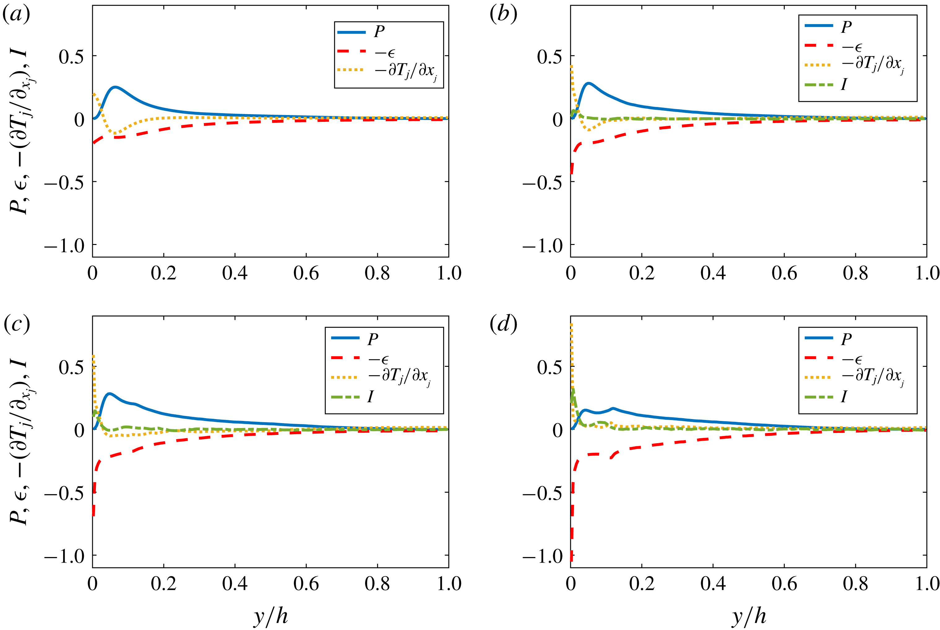
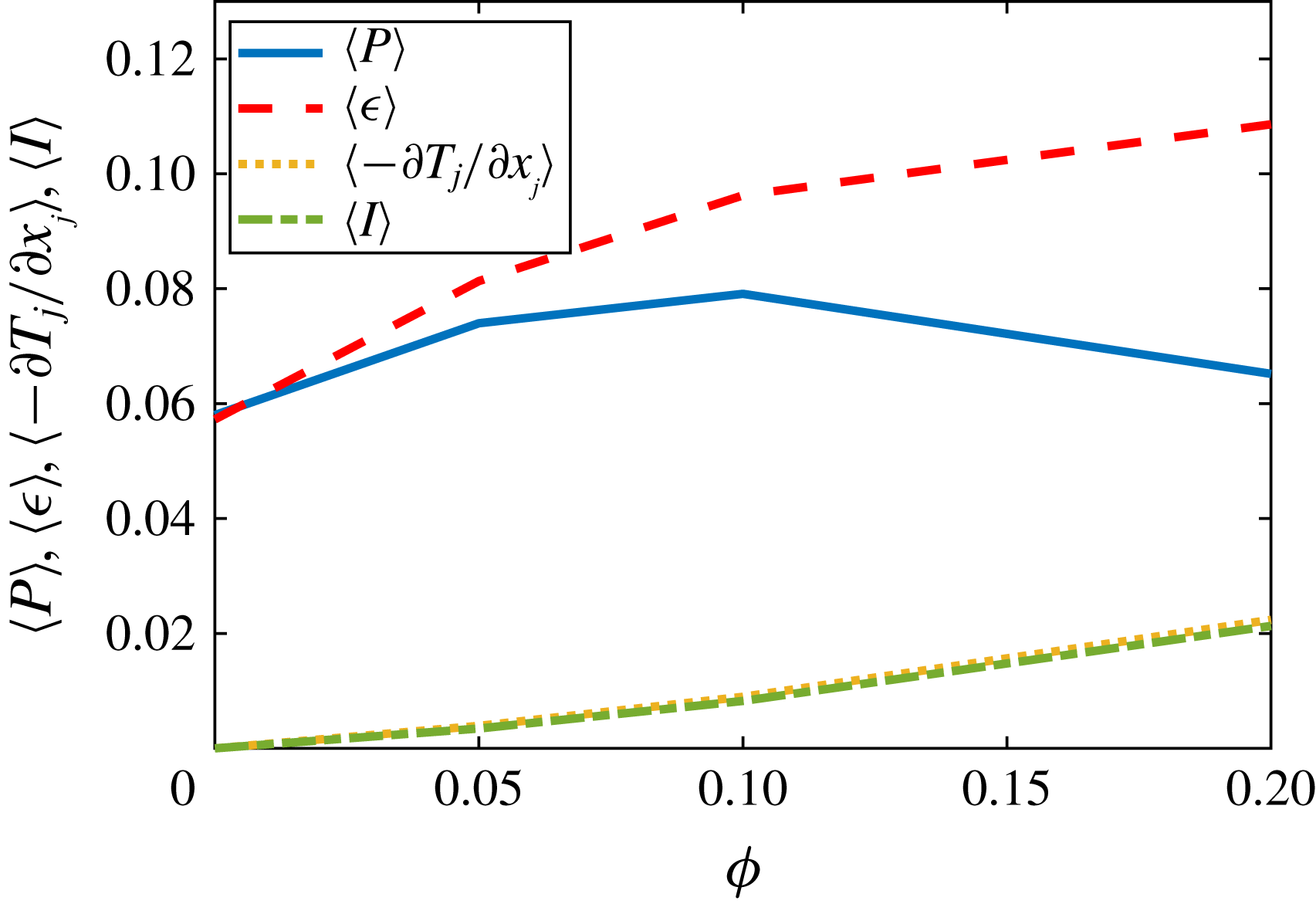
the turbulence activity may be more strongly reduced in duct flow than in channel flow. We tend towards the second hypothesis, as in duct flow twice as many particles are found in the near-wall regions than in channel flow. Due to the large concentration of particles, the quasi-coherent structures are quickly disrupted, ejection and sweep events reduce and the overall production of turbulent kinetic energy is reduced. To support this idea, we also perform a turbulent kinetic energy budget and, indeed, find that the mean turbulence production increases only up to
 $\unicode[STIX]{x1D719}=0.1$
. Instead, for
 $\unicode[STIX]{x1D719}=0.2$
the mean production is less than for
 $\unicode[STIX]{x1D719}=0.05$
. On the other hand, the mean dissipation and transport increase substantially with
 $\unicode[STIX]{x1D719}$
. Due to the presence of solid particles, there is an additional contribution to the turbulent kinetic energy budget: the interphase interaction term. We find that it contributes positively to the budget, and that its mean value increases monotonically with the volume fraction, similarly to the mean transport term. In addition, this term is particularly important very close to the walls, in the viscous sublayer.
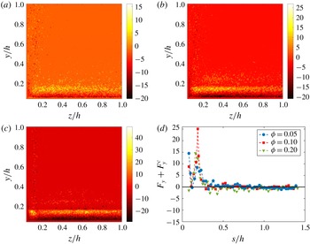
Finally, we compute the slip velocity between fluid and particles, and the mean wall-normal hydrodynamic and collision forces acting on the particles. We find that particles move on average faster than the fluid. However, there are several regions where they lag behind it. This occurs, for example, close to the corners. Interestingly, it is found that along the corner bisectors, the slip velocity vanishes where the maxima of particle concentration are found (for
 $\unicode[STIX]{x1D719}=0.05$
and 0.1). From the mean hydrodynamic and collision forces, it is found that particles are repelled from the corners, and the summation of these forces vanishes around the locations of maximum concentration. For
 $\unicode[STIX]{x1D719}=0.2$
, although the mean hydrodynamic forces are generally negligible in the core region, these are slightly negative along the bisectors (i.e. directed towards the walls). However, at large
 $\unicode[STIX]{x1D719}$
the motion of particles is hindered by collisions with their neighbours. Hence, along the corner bisectors particles experience collision forces that balance the hydrodynamic forces. The mean total force on the particles is therefore (approximately) zero, and this explains the large concentration at the core.
2 Methodology
2.1 Numerical method
During the last years, various methods have been proposed to perform interface-resolved direct numerical simulations (DNS) of particulate flows. The state of art and the different principles and applications have been recently documented in the comprehensive review article by Maxey (Reference Maxey2017). In the present study, the immersed boundary method (IBM) originally proposed by Uhlmann (Reference Uhlmann2005) and modified by Breugem (Reference Breugem2012) has been used to simulate suspensions of finite-size neutrally buoyant spherical particles in turbulent square duct flow. The fluid phase is described in an Eulerian framework by the incompressible Navier–Stokes equations:
 $$\begin{eqnarray}\displaystyle & \displaystyle \unicode[STIX]{x1D735}\boldsymbol{\cdot }\boldsymbol{u}_{f}=0, & \displaystyle\end{eqnarray}$$
 $$\begin{eqnarray}\displaystyle & \displaystyle \frac{\unicode[STIX]{x2202}\boldsymbol{u}_{f}}{\unicode[STIX]{x2202}t}+\boldsymbol{u}_{f}\boldsymbol{\cdot }\unicode[STIX]{x1D735}\boldsymbol{u}_{f}=-\frac{1}{\unicode[STIX]{x1D70C}_{f}}\unicode[STIX]{x1D735}p+\unicode[STIX]{x1D708}\unicode[STIX]{x1D6FB}^{2}\boldsymbol{u}_{f}+\boldsymbol{f}, & \displaystyle\end{eqnarray}$$
where
 $\boldsymbol{u}_{f}$
and
 $p$
are the velocity field and pressure, while
 $\unicode[STIX]{x1D70C}_{f}$
and
 $\unicode[STIX]{x1D708}$
are the density and kinematic viscosity of the fluid phase. The last term on the right-hand side of (2.2)
 $\boldsymbol{f}$
is the localized IBM force imposed to the flow to model the boundary condition at the moving particle surface (i.e.
 $\boldsymbol{u}_{f}|_{\unicode[STIX]{x2202}{\mathcal{V}}_{p}}=\boldsymbol{u}_{p}+\unicode[STIX]{x1D74E}_{p}\times \boldsymbol{r}$
). The dynamics of the rigid particles is determined by the Newton–Euler Lagrangian equations:
 $$\begin{eqnarray}\displaystyle & \displaystyle \unicode[STIX]{x1D70C}_{p}V_{p}\frac{\text{d}\boldsymbol{u}_{p}}{\text{d}t}=\oint _{\unicode[STIX]{x2202}{\mathcal{V}}_{p}}\unicode[STIX]{x1D749}\boldsymbol{\cdot }\boldsymbol{n}\,\text{d}S+\boldsymbol{F}^{c}, & \displaystyle\end{eqnarray}$$
 $$\begin{eqnarray}\displaystyle & \displaystyle I_{p}\frac{\text{d}\unicode[STIX]{x1D74E}_{p}}{\text{d}t}=\oint _{\unicode[STIX]{x2202}{\mathcal{V}}_{p}}\boldsymbol{r}\times \unicode[STIX]{x1D749}\boldsymbol{\cdot }\boldsymbol{n}\,\text{d}S+\boldsymbol{T}^{c}, & \displaystyle\end{eqnarray}$$
where
 $\boldsymbol{u}_{p}$
and
 $\unicode[STIX]{x1D74E}_{p}$
are the linear and angular velocities of the particle, while
 $\boldsymbol{F}^{c}$
and
 $\boldsymbol{T}^{c}$
are the collision forces and torques (due to particle–particle and particle–wall interactions). In (2.3) and (2.4),
 $V_{p}=4\unicode[STIX]{x03C0}a^{3}/3$
and
 $I_{p}=2\unicode[STIX]{x1D70C}_{p}V_{p}a^{2}/5$
represent the particle volume and moment of inertia,
 $\unicode[STIX]{x1D749}=-p\boldsymbol{I}+\unicode[STIX]{x1D708}\unicode[STIX]{x1D70C}_{f}(\unicode[STIX]{x1D735}\boldsymbol{u}_{f}+\unicode[STIX]{x1D735}\boldsymbol{u}_{f}^{\text{T}})$
is the fluid stress tensor,
 $\boldsymbol{r}$
indicates the distance from the centre of the particle and
 $\boldsymbol{n}$
is the unit vector normal to the particle surface
 $\unicode[STIX]{x2202}{\mathcal{V}}_{p}$
.
In order to solve the governing equations, the fluid phase is discretized on a spatially uniform staggered Cartesian grid using a second-order finite-difference scheme. An explicit third-order Runge–Kutta scheme is combined with a standard pressure-correction method to perform the time integration at each sub-step. The same time integration scheme has also been used for the evolution of (2.3) and (2.4). For the solid phase, each particle surface is described by
 $N_{L}$
uniformly distributed Lagrangian points. The force exchanged by the fluid on the particles is imposed on each
 $l$
th Lagrangian point. This force is related to the Eulerian force field
 $\boldsymbol{f}$
by the expression
 $\boldsymbol{f}_{ijk}=\sum _{l=1}^{N_{L}}\boldsymbol{F}_{l}\unicode[STIX]{x1D6FF}_{d}(x_{ijk}-\boldsymbol{X}_{l})\unicode[STIX]{x0394}V_{l}$
, where
 $\unicode[STIX]{x0394}V_{l}$
is the volume of the cell containing the
 $l$
th Lagrangian point and
 $\unicode[STIX]{x1D6FF}_{d}$
is the regularized Dirac delta function (Roma, Peskin & Berger Reference Roma, Peskin and Berger1999). This is defined as the product of
 $3$
one-dimensional delta functions (one in each direction),
 $\unicode[STIX]{x1D6FF}_{d}^{1}(x_{i}-X_{l,i})=\unicode[STIX]{x1D709}(r_{d})/\unicode[STIX]{x0394}x_{i}$
, with
 $$\begin{eqnarray}\displaystyle \unicode[STIX]{x1D709}(r_{d})\left\{\begin{array}{@{}ll@{}}{\textstyle \frac{1}{6}}(5-3|r_{d}|-\sqrt{(-3(1-|r_{d}|)^{2}+1)}),\quad & 0.5\leqslant |r_{d}|\leqslant 1.5,\\ {\textstyle \frac{1}{3}}(1+\sqrt{(-3{r_{d}}^{2}+1)}),\quad & |r_{d}|\leqslant 0.5,\\ 0\quad & \text{otherwise}\end{array}\right. & & \displaystyle\end{eqnarray}$$
and
 $r_{d}=(x_{i}-X_{l,i})/\unicode[STIX]{x0394}x_{i}$
. Here,
 $\boldsymbol{F}_{l}$
is the force (per unit mass) at each Lagrangian point, and it is computed as
 $\boldsymbol{F}_{l}=(\boldsymbol{U}_{p}(\boldsymbol{X}_{l})-\boldsymbol{U}_{l}^{\ast })/\unicode[STIX]{x0394}t$
, where
 $\boldsymbol{U}_{p}=\boldsymbol{u}_{p}+\unicode[STIX]{x1D74E}_{p}\times \boldsymbol{r}$
is the velocity at the Lagrangian point
 $l$
at the previous time step, while
 $\boldsymbol{U}_{l}^{\ast }$
is the interpolated first prediction velocity at the same point. An iterative algorithm with second-order spatial accuracy is developed to calculate this force field. To maintain accuracy, equations (2.3) and (2.4) are rearranged in terms of the IBM force field,
 $$\begin{eqnarray}\displaystyle & \displaystyle \unicode[STIX]{x1D70C}_{p}V_{p}\frac{\text{d}\boldsymbol{u}_{p}}{\text{d}t}=-\unicode[STIX]{x1D70C}_{f}\mathop{\sum }_{l=1}^{N_{l}}\boldsymbol{F}_{l}\unicode[STIX]{x0394}V_{l}+\unicode[STIX]{x1D70C}_{f}\frac{\text{d}}{\text{d}t}\int _{{\mathcal{V}}_{p}}\boldsymbol{u}_{f}\,\text{d}V+\boldsymbol{F}^{c}, & \displaystyle\end{eqnarray}$$
 $$\begin{eqnarray}\displaystyle & \displaystyle I_{p}\frac{\text{d}\unicode[STIX]{x1D74E}_{p}}{\text{d}t}=-\unicode[STIX]{x1D70C}_{f}\mathop{\sum }_{l=1}^{N_{l}}\boldsymbol{r}_{l}\times \boldsymbol{F}_{l}\unicode[STIX]{x0394}V_{l}+\unicode[STIX]{x1D70C}_{f}\frac{\text{d}}{\text{d}t}\int _{{\mathcal{V}}_{p}}\boldsymbol{r}\times \boldsymbol{u}_{f}\,\text{d}V+\boldsymbol{T}^{c}, & \displaystyle\end{eqnarray}$$
where
 $\boldsymbol{r}_{l}$
is the distance between the centre of a particle and the
 $l$
th Lagrangian point on its surface. The second terms on the right-hand sides are corrections that account for the inertia of the fictitious fluid contained within the particle volume. Particle–particle and particle–wall interactions are also considered. Well-known models based on Brenner’s asymptotic solution (Brenner Reference Brenner1961) are employed to correctly predict the lubrication force when the distance between particles as well as particles and walls is smaller than twice the mesh size. Collisions are modelled using a soft-sphere collision model, with a coefficient of restitution of 0.97 to achieve an almost elastic rebound of particles. Friction forces are also taken into account (Costa et al.
Reference Costa, Boersma, Westerweel and Breugem2015). For more detailed discussions of the numerical method and of the mentioned models the reader is refereed to previous publications (Breugem Reference Breugem2012; Picano et al.
Reference Picano, Breugem and Brandt2015; Fornari et al.
Reference Fornari, Formenti, Picano and Brandt2016b
; Fornari, Picano & Brandt Reference Fornari, Picano and Brandt2016c
; Lashgari et al.
Reference Lashgari, Picano, Breugem and Brandt2016).
Periodic boundary conditions for both solid and liquid phases are imposed in the streamwise direction. The stress immersed boundary method is used in the remaining directions to impose the no-slip/no-penetration conditions at the duct walls. The stress immersed boundary method has originally been developed to simulate the flow around rectangular-shaped obstacles in a fully Cartesian grid (Breugem, Van Dijk & Delfos Reference Breugem, Van Dijk and Delfos2014). In this work, we use this method to enforce the fluid velocity to be zero at the duct walls. For more details on the method, the reader is referred to the works of Breugem & Boersma (Reference Breugem and Boersma2005) and Pourquie, Breugem & Boersma (Reference Pourquie, Breugem and Boersma2009). This approach has already been used in our group (Kazerooni et al. Reference Kazerooni, Fornari, Hussong and Brandt2017) to study the laminar flow of large spheres in a squared duct.
2.2 Flow geometry
We investigate the turbulent flow of dense suspensions of neutrally buoyant spherical particles in a square duct. The simulations are performed in a Cartesian computational domain of size
 $L_{x}=12h$
,
 $L_{z}=2h$
and
 $L_{y}=2h$
where
 $h$
is the duct half-width and
 $x$
,
 $y$
and
 $z$
are the streamwise and cross-stream directions. The domain is uniformly (
 $\unicode[STIX]{x0394}x=\unicode[STIX]{x0394}z=\unicode[STIX]{x0394}y$
) meshed by
 $2592\times 432\times 432$
Eulerian grid points in the streamwise and cross-flow directions. The bulk velocity of the entire mixture
 $U_{b}$
is kept constant by adjusting the streamwise pressure gradient to achieve the constant bulk Reynolds number
 $Re_{b}=U_{b}2h/\unicode[STIX]{x1D708}=5600$
. In particular, we fix a constant reference value of the bulk velocity
 $U_{b}$
, and at each time step compute the spatial average of the mixture velocity. From these quantities we hence find the pressure gradient necessary to constrain the mixture to move with velocity equal to
 $U_{b}$
. Based on the data provided by Pinelli et al. (Reference Pinelli, Uhlmann, Sekimoto and Kawahara2010),
 $Re_{b}=5600$
corresponds to a mean friction Reynolds number
 $Re_{\unicode[STIX]{x1D70F}}=\bar{U}_{\ast }h/\unicode[STIX]{x1D708}=185$
for an unladen case, where
 $\bar{U}_{\ast }=\sqrt{\langle \unicode[STIX]{x1D70F}_{w}\rangle /\unicode[STIX]{x1D70C}_{f}}$
is the friction velocity calculated using the mean value of the shear stress
 $\unicode[STIX]{x1D70F}_{w}$
along the duct walls.
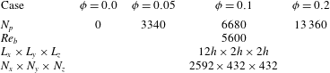
We consider three different solid volume fractions of
 $\unicode[STIX]{x1D719}=5,10$
and 20 % which correspond to 3340, 6680 and 13 360 particles respectively. The reference unladen case is also considered for direct comparison. In all simulations, the duct-to-particle size ratio is fixed to
 $h/a=18$
, and the particles are randomly initialized in the computational domain with zero translational and angular velocities. The number of Eulerian grid points per particle diameter is 24 (
 $\unicode[STIX]{x0394}x=1/24$
) whereas the Lagrangian mesh on the surface of the particles consists of 1721 grid points.
The simulations start from the laminar duct flow and the noise introduced by a high amplitude localised disturbance in the form of two counter-rotating streamwise vortices (Henningson & Kim Reference Henningson and Kim1991). Due to this disturbance and to the noise added by the particles, transition naturally occurs at the chosen Reynolds number. The statistics are collected after the initial transient phase of approximately
 $100\,h/U_{b}$
, using an averaging period of at least
 $600\,h/U_{b}$
(Huser & Biringen Reference Huser and Biringen1993; Vinuesa et al.
Reference Vinuesa, Noorani, Lozano-Durán, Khoury, Schlatter, Fischer and Nagib2014) (except for
 $\unicode[STIX]{x1D719}=20\,\%$
where
 ${\sim}400\,h/U_{b}$
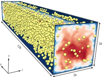
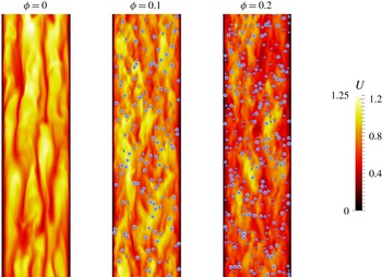
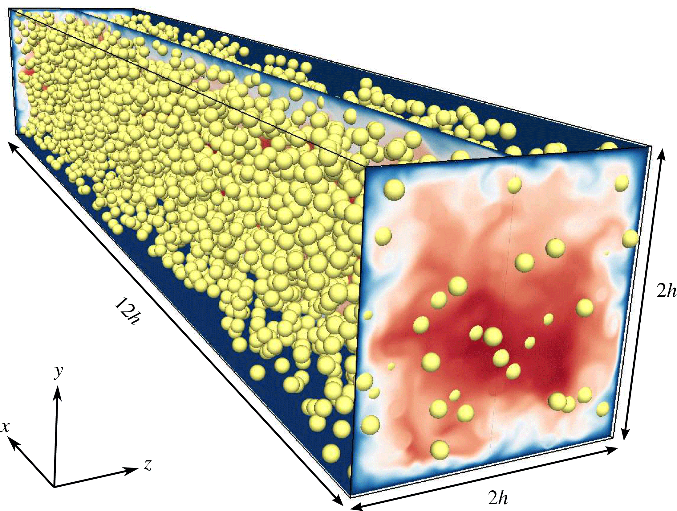
is found to be enough to obtain converged statistics). A summary of the simulations is presented in table 1 while an instantaneous snapshot showing the magnitude of the streamwise velocity for
 $\unicode[STIX]{x1D719}=0.1$
, together with the solid particles, is shown in figure 1.
Instantaneous snapshot of the magnitude of the velocity together with the solid particles; the solid volume fraction
 $\unicode[STIX]{x1D719}=0.1$
.
Summary of the different simulation cases.
 $N_{p}$
indicates the number of particles whereas
 $N_{x}$
,
 $N_{y}$
and
 $N_{z}$
are the number of grid points in each direction.

3 Results
3.1 Validation
The code used in the present work has been already validated against several different cases in previous studies (Breugem Reference Breugem2012; Picano et al.
Reference Picano, Breugem and Brandt2015; Fornari et al.
Reference Fornari, Picano and Brandt2016c
; Kazerooni et al.
Reference Kazerooni, Fornari, Hussong and Brandt2017). To further investigate the accuracy of the code, we calculate the friction factor
 $f=8(\bar{U}_{\ast }/U_{b})^{2}$
for the reference unladen case with
 $Re_{b}=5600$
, and compare it with the value obtained from the empirical correlation by Jones (Reference Jones1976)
 $$\begin{eqnarray}\displaystyle 1/f^{2}=2\log _{10}(1.125Re_{b}f^{1/2})-0.8. & & \displaystyle\end{eqnarray}$$
The same value of
 $f=0.035$
is obtained from the simulation and the empirical formula. This corresponds to a mean
 $Re_{\unicode[STIX]{x1D70F}}=185$
.
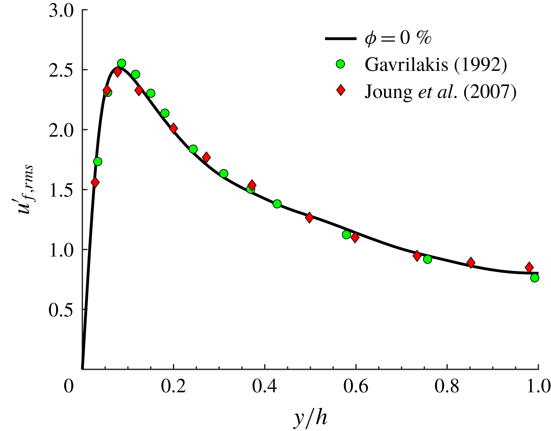
We also performed a simulation at lower
 $Re_{b}=4410$
and
 $\unicode[STIX]{x1D719}=0$
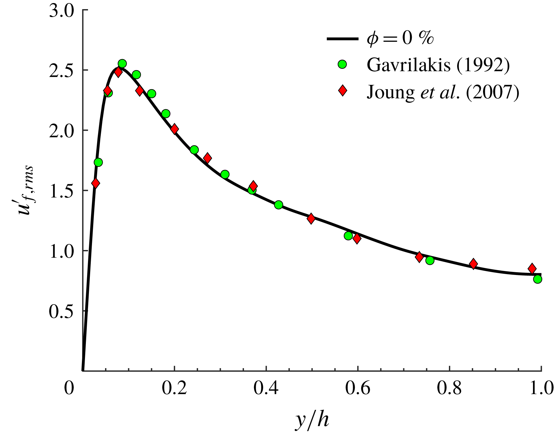
, see figure 2, where we report the profile of the streamwise velocity fluctuation at the wall bisector, normalized by the local friction velocity
 $U_{\ast }$
. This is compared to the results by Gavrilakis (Reference Gavrilakis1992) and Joung, Choi & Choi (Reference Joung, Choi and Choi2007) at
 $Re_{b}=4410$
and 4440. We see a good agreement with both works. For all components of the root-mean-square velocity, the relative difference between our results (at the wall bisector) and those by Gavrilakis (Reference Gavrilakis1992) is typically less than 1.5 % (and at most 4 % locally).
Streamwise velocity fluctuation at the wall bisector from the present simulation at
 $Re_{b}=4410$
, and from the data by Gavrilakis (Reference Gavrilakis1992) at
 $Re_{b}=4410$
and Joung et al. (Reference Joung, Choi and Choi2007) at
 $Re_{b}=4440$
.
3.2 Mean velocities, drag and particle concentration
In this section we report and discuss the results obtained for the different solid volume fractions
 $\unicode[STIX]{x1D719}$
considered. The phase ensemble averages for the fluid (solid) phase have been calculated by considering only the points located outside (inside) of the volume occupied by the particles. The statistics reported are obtained by further averaging over the eight symmetric triangles that form the duct cross-section.
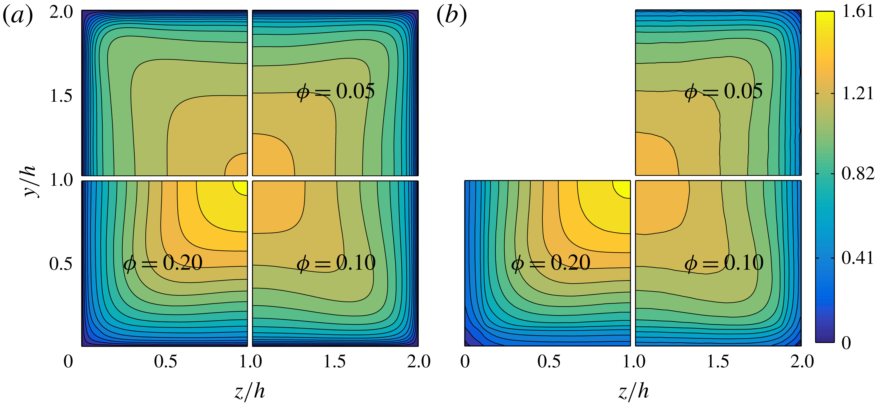
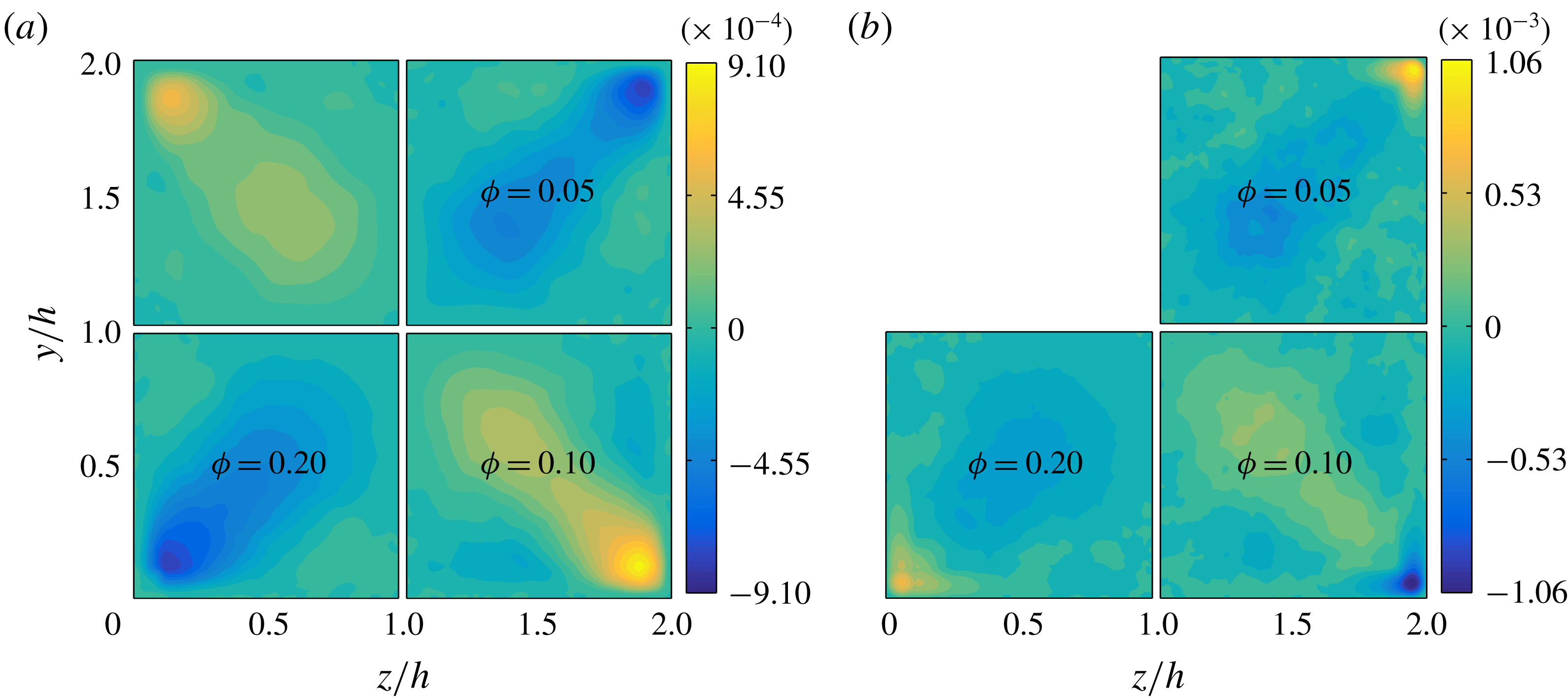
The streamwise mean fluid and particle velocities in outer units (i.e. normalized by the bulk velocity
 $U_{b}$
),
 $U_{f/p}(y,z)$
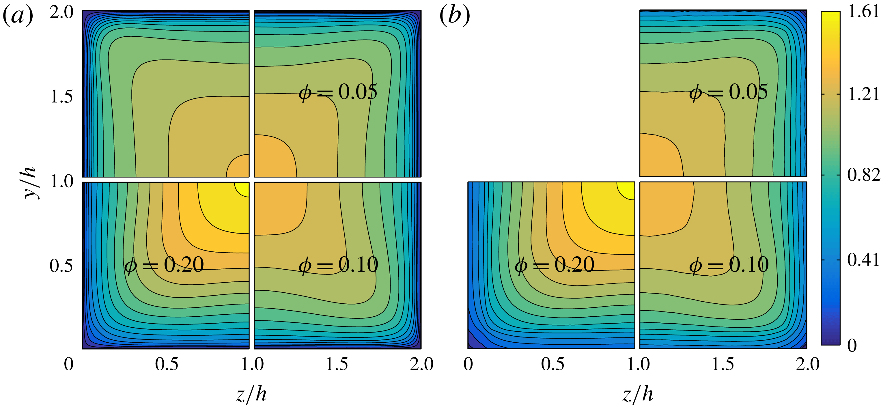
, are illustrated in figure 3(a,b) for all
 $\unicode[STIX]{x1D719}$
. The contour plots are divided in four quadrants showing results for
 $\unicode[STIX]{x1D719}=0.0$
(top left), 0.05 (top right), 0.1 (bottom right) and
 $0.2$
(bottom left). The streamwise mean particle velocity contours closely resemble those of the fluid phase. In particular we observe that the maximum velocity at the core of the duct grows with
 $\unicode[STIX]{x1D719}$
. The increase with
 $\unicode[STIX]{x1D719}$
is similar to that reported for turbulent channel flows (Picano et al.
Reference Picano, Breugem and Brandt2015), except for
 $\unicode[STIX]{x1D719}=0.2$
where the increase of
 $U_{f/p}(y,z)$
in the duct core is substantially larger. We observe that the convexity of the mean velocity contours also increases with the volume fraction up to
 $\unicode[STIX]{x1D719}=0.1$
. This is due to the increased intensity of secondary flows that convect mean velocity from regions of large shear along the walls towards regions of low shear along the corner bisectors (Prandtl Reference Prandtl1963; Gessner Reference Gessner1973; Vinuesa et al.
Reference Vinuesa, Noorani, Lozano-Durán, Khoury, Schlatter, Fischer and Nagib2014). For
 $\unicode[STIX]{x1D719}=0.2$
the secondary flow intensity is substantially reduced and accordingly also the convexity of the contours of
 $U_{f/p}$
reduces.
Contours of streamwise mean fluid (a) and particle velocity (b) in outer units. In each figure, the top left, top right, bottom right and bottom left quadrants show the data for
 $\unicode[STIX]{x1D719}=0.0,0.05,0.1$
and 0.2.
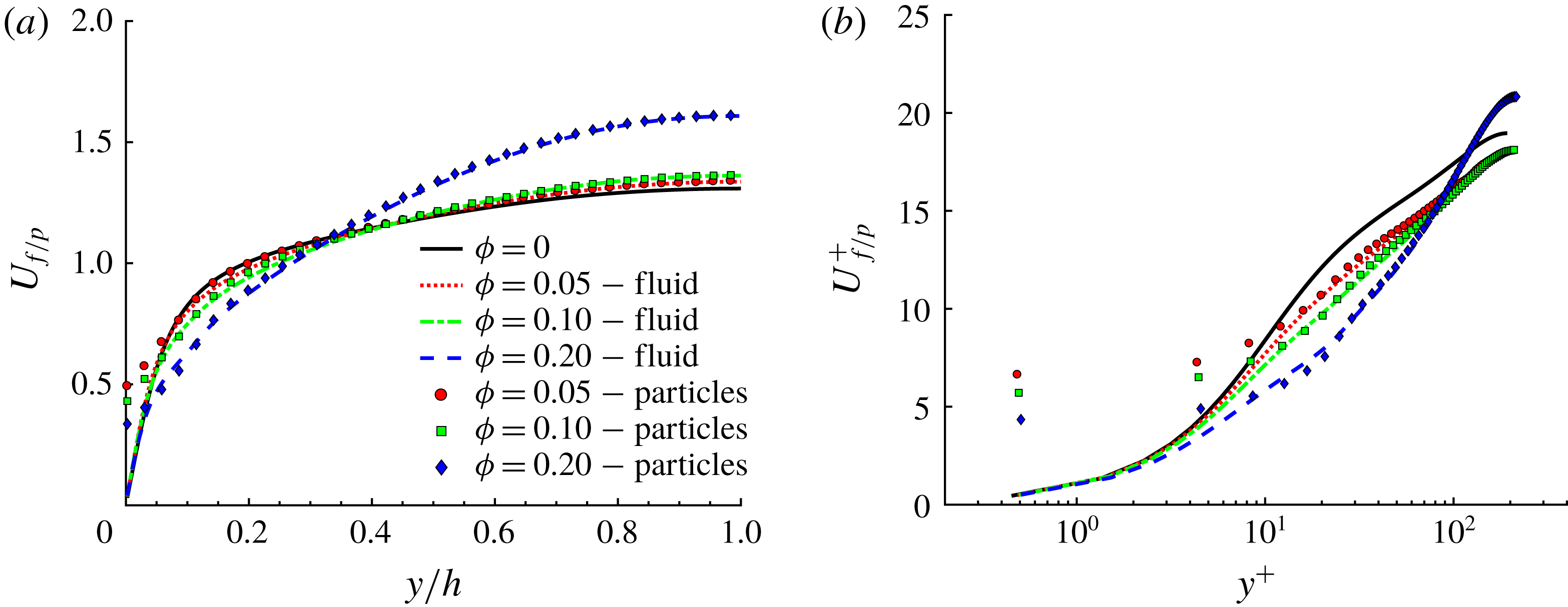
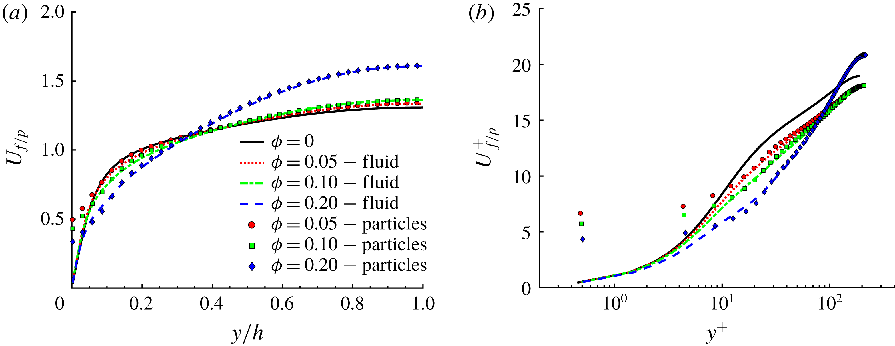
Next, we show in figure 4(a,b) the streamwise mean fluid and particle velocity profiles along the wall bisector in outer and inner units (
 $U_{f/p}(y)$
and
 $U_{f/p}^{+}$
). The local value of the friction velocity at the wall bisector,
 $U_{\ast }=\sqrt{\unicode[STIX]{x1D70F}_{w,bis}/\unicode[STIX]{x1D70C}_{f}}$
, is used to normalize
 $U_{f/p}(y)$
. Solid lines are used for
 $U_{f}(y)$
while symbols are used for
 $U_{p}(y)$
. We observe that the mean velocity profiles of the two phases are almost perfectly overlapping at equal
 $\unicode[STIX]{x1D719}$
, except very close to the walls (
 $y^{+}\leqslant 30$
) where particles have a relative tangential motion (slip velocity). Note also that the mean particle velocity decreases with
 $\unicode[STIX]{x1D719}$
very close to the walls. We also observe that by increasing
 $\unicode[STIX]{x1D719}$
, the profiles of
 $U_{f/p}(y)$
tend towards the laminar parabolic profile with lower velocity near the wall and larger velocity at the centreline,
 $y/h=1$
. Concerning
 $U_{f/p}^{+}(y^{+})$
, we observe a progressive downward shift of the profiles with the volume fraction
 $\unicode[STIX]{x1D719}$
denoting a drag increase, at least up to
 $\unicode[STIX]{x1D719}=0.1$
.
The mean velocity profiles still follow the log law (Pope Reference Pope2000)
 $$\begin{eqnarray}\displaystyle U_{f/p}^{+}(y^{+})=\frac{1}{k}\log (y^{+})+B, & & \displaystyle\end{eqnarray}$$
where
 $k$
is the von Kármán constant and
 $B$
is an additive coefficient. For the unladen case with
 $Re_{b}=4410$
, Gavrilakis (Reference Gavrilakis1992) fitted the data between
 $y^{+}=30$
and 100 to find
 $k=0.31$
and
 $B=3.9$
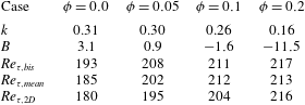
. In the present simulations, the extent of the log region is larger due to the higher bulk Reynolds number and we hence fit our data between
 $y^{+}=30$
and 140. The results are reported in table 2. For the unladen case we obtain results in agreement with those of Gavrilakis (Reference Gavrilakis1992) although our constant
 $B$
is slightly smaller. Increasing
 $\unicode[STIX]{x1D719}$
,
 $k$
decreases and the additive constant
 $B$
decreases becoming negative at
 $\unicode[STIX]{x1D719}=0.1$
. Values for
 $k$
and
 $B$
are also reported for
 $\unicode[STIX]{x1D719}=0.2$
in table 2, although a log layer cannot be clearly identified.
Streamwise mean fluid and particle velocity along the wall bisector at
 $z/h=1$
in outer (a) and inner units (b). Lines are used for fluid velocity profiles while symbols are used for particle velocity profiles.
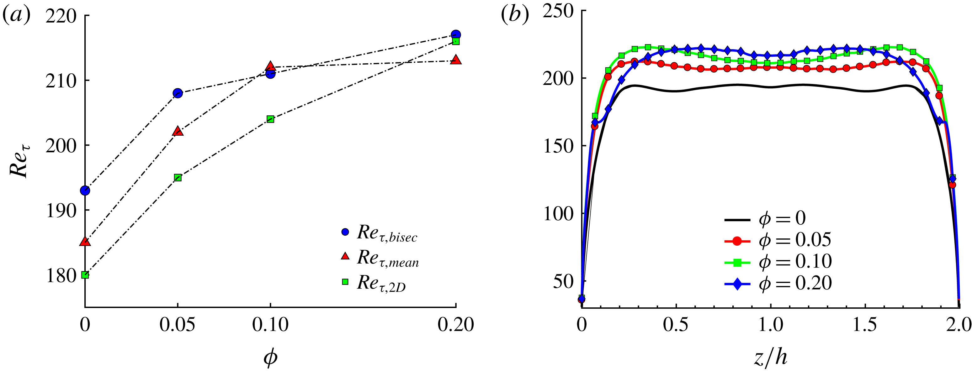
(a) Mean friction Reynolds number
 $Re_{\unicode[STIX]{x1D70F},mean}$
estimated from the pressure gradient, friction Reynolds number at the wall bisector
 $Re_{\unicode[STIX]{x1D70F},bis}$
and mean friction Reynolds number for the channel flow,
 $Re_{\unicode[STIX]{x1D70F},2D}$
(Picano et al.
Reference Picano, Breugem and Brandt2015), for all volume fractions
 $\unicode[STIX]{x1D719}$
. (b) Profile of
 $Re_{\unicode[STIX]{x1D70F}}$
along the duct wall.
The von Kármán constant and additive constant
 $B$
of the log law at the wall bisector estimated from the present simulations for different volume fractions
 $\unicode[STIX]{x1D719}$
. Here
 $k$
and
 $B$
have been fitted in the range
 $y^{+}\in [30,140]$
. The friction Reynolds number calculated at the wall bisector
 $Re_{\unicode[STIX]{x1D70F},bis}$
, the mean friction Reynolds number
 $Re_{\unicode[STIX]{x1D70F},mean}$
estimated via the pressure gradient, and the corresponding friction Reynolds number found by Picano et al. (Reference Picano, Breugem and Brandt2015) for turbulent channel flow,
 $Re_{\unicode[STIX]{x1D70F},2D}$
, are also reported.
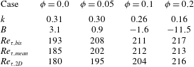
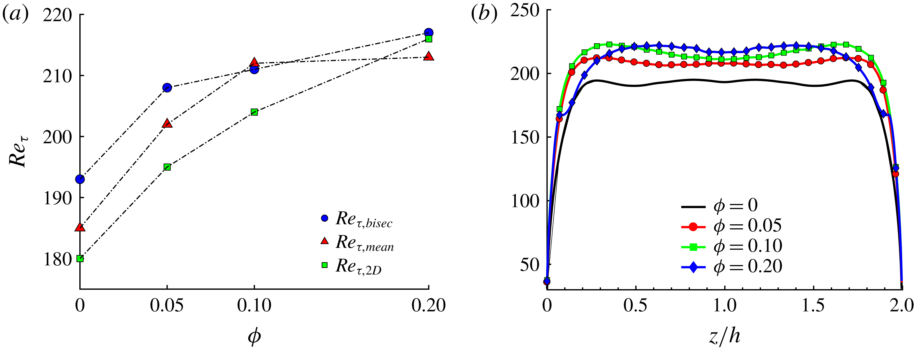
At the wall bisector, we also calculated the local friction Reynolds
 $Re_{\unicode[STIX]{x1D70F},bis}$
. This is reported in figure 5(a) and in table 2 as function of the volume fraction
 $\unicode[STIX]{x1D719}$
. The results of Picano et al. (Reference Picano, Breugem and Brandt2015) are also reported for comparison in table 2. We see that although the initial value of
 $Re_{\unicode[STIX]{x1D70F},bis}$
for
 $\unicode[STIX]{x1D719}=0.0$
is substantially larger than that of the corresponding channel flow at
 $Re_{b}=5600$
, the increase with the volume fraction is smaller than for
 $Re_{\unicode[STIX]{x1D70F},2D}$
. Indeed for
 $\unicode[STIX]{x1D719}=0.2$
we find that
 $Re_{\unicode[STIX]{x1D70F},bis}\simeq Re_{\unicode[STIX]{x1D70F},2D}$
. In the absence of particles, the increase of
 $Re_{\unicode[STIX]{x1D70F},bis}$
with respect to
 $Re_{\unicode[STIX]{x1D70F},2D}$
is due to the fact that here the secondary flows are directed towards the core, transporting streamwise momentum in the wall-normal direction, therefore inducing a steeper gradient,
 $\text{d}U_{f}/\text{d}y$
.
It is also interesting to observe the behaviour of the mean friction Reynolds number
 $Re_{\unicode[STIX]{x1D70F},mean}$
as a function of
 $\unicode[STIX]{x1D719}$
, as this directly relates to the overall pressure drop along the duct. For each case, we estimate the wall shear stress directly via the pressure gradient needed to drive the flow (
 $\langle \unicode[STIX]{x1D70F}_{w}\rangle =-(\text{d}P/\text{d}x)L_{z}/4$
). From the shear stress we then compute the mean friction Reynolds number. From figure 5(a) and table 2 we see that
 $Re_{\unicode[STIX]{x1D70F},mean}$
strongly increases with the volume fraction up to
 $\unicode[STIX]{x1D719}=0.1$
. The increase in
 $Re_{\unicode[STIX]{x1D70F},mean}$
with
 $\unicode[STIX]{x1D719}$
is similar to that observed for
 $Re_{\unicode[STIX]{x1D70F},2D}$
in channel flow. However, by further increasing the volume fraction to
 $\unicode[STIX]{x1D719}=0.2$
,
 $Re_{\unicode[STIX]{x1D70F},mean}$
remains approximately constant in duct flow (it actually increases by 0.5 % as
 $\unicode[STIX]{x1D719}$
increases from 0.1 to 0.2), while it increases by
 ${\sim}6\,\%$
in channel flow. It is also interesting to note that
 $Re_{\unicode[STIX]{x1D70F},mean}$
would be underestimated if only computed via the mean fluid streamwise velocity gradient at the walls. Indeed, the wall friction is altered by the shear exerted by the particles on the walls (through lubrication and collisions). This is particularly important for
 $\unicode[STIX]{x1D719}=0.2$
. At this
 $\unicode[STIX]{x1D719}$
,
 $Re_{\unicode[STIX]{x1D70F},mean}$
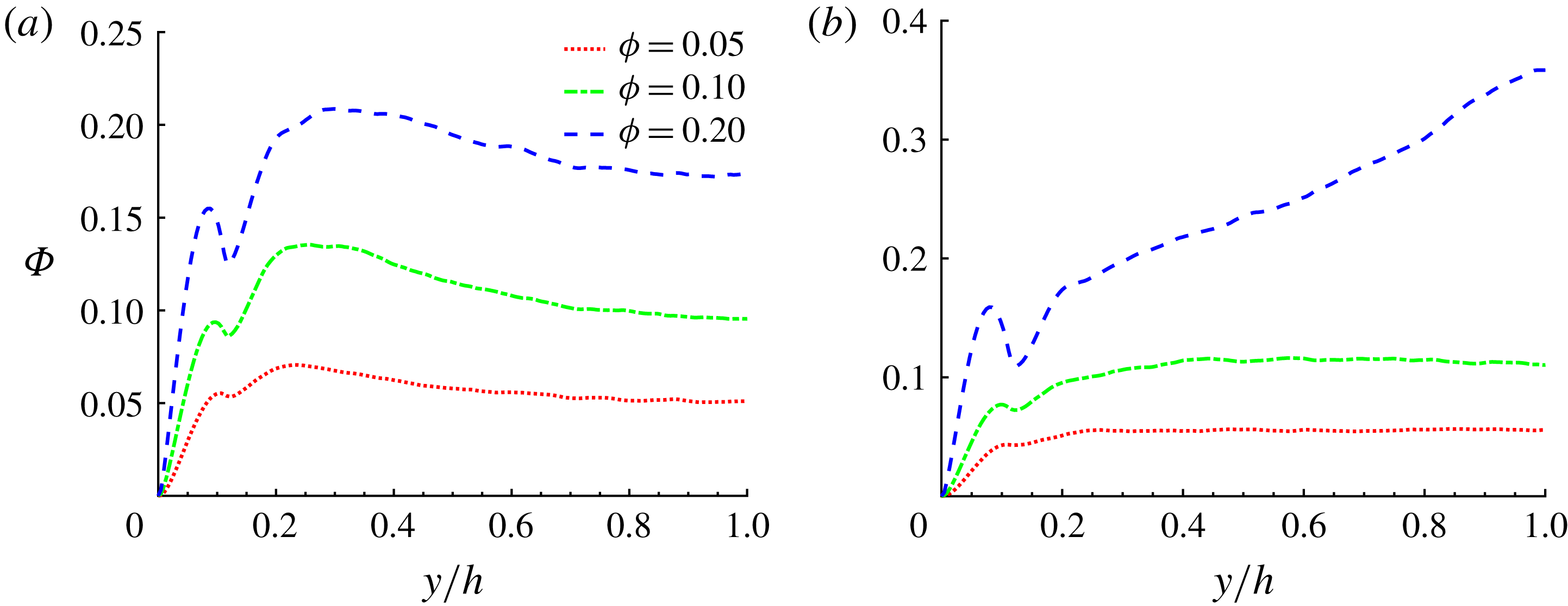
would be underestimated by approximately 3 %. In figure 5(b) we report the profiles of
 $Re_{\unicode[STIX]{x1D70F}}$
, displaying the signature of the near-wall structures (estimated by the velocity gradient) along one wall. We note that the friction Reynolds number increases with
 $\unicode[STIX]{x1D719}$
, especially towards the corners. For
 $\unicode[STIX]{x1D719}=0.2$
, instead, the profile exhibits a sharp change at approximately
 $z/h=0.1\sim 2a$
, and the maxima move towards the wall bisector (
 $z/h\sim 0.65$
). This is probably due to the clear change in local particle concentration in the cross-section as we will explain in the following.
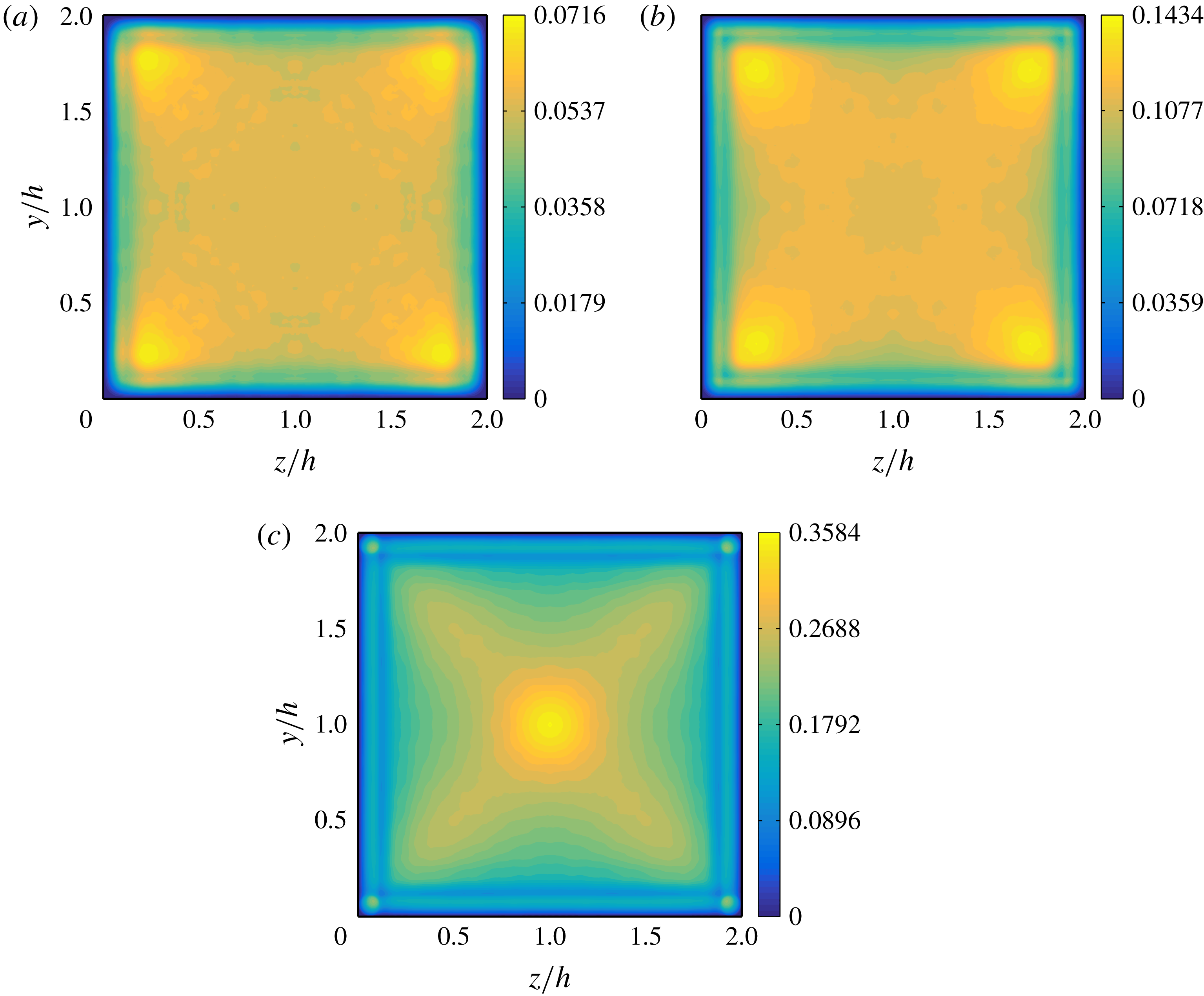
Mean particle concentration
 $\unicode[STIX]{x1D6F7}(y,z)$
in the duct cross-section for
 $\unicode[STIX]{x1D719}=0.05$
(a),
 $\unicode[STIX]{x1D719}=0.1$
(b) and
 $\unicode[STIX]{x1D719}=0.2$
(c).
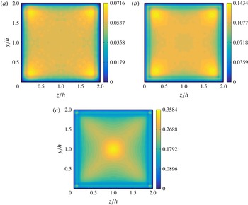
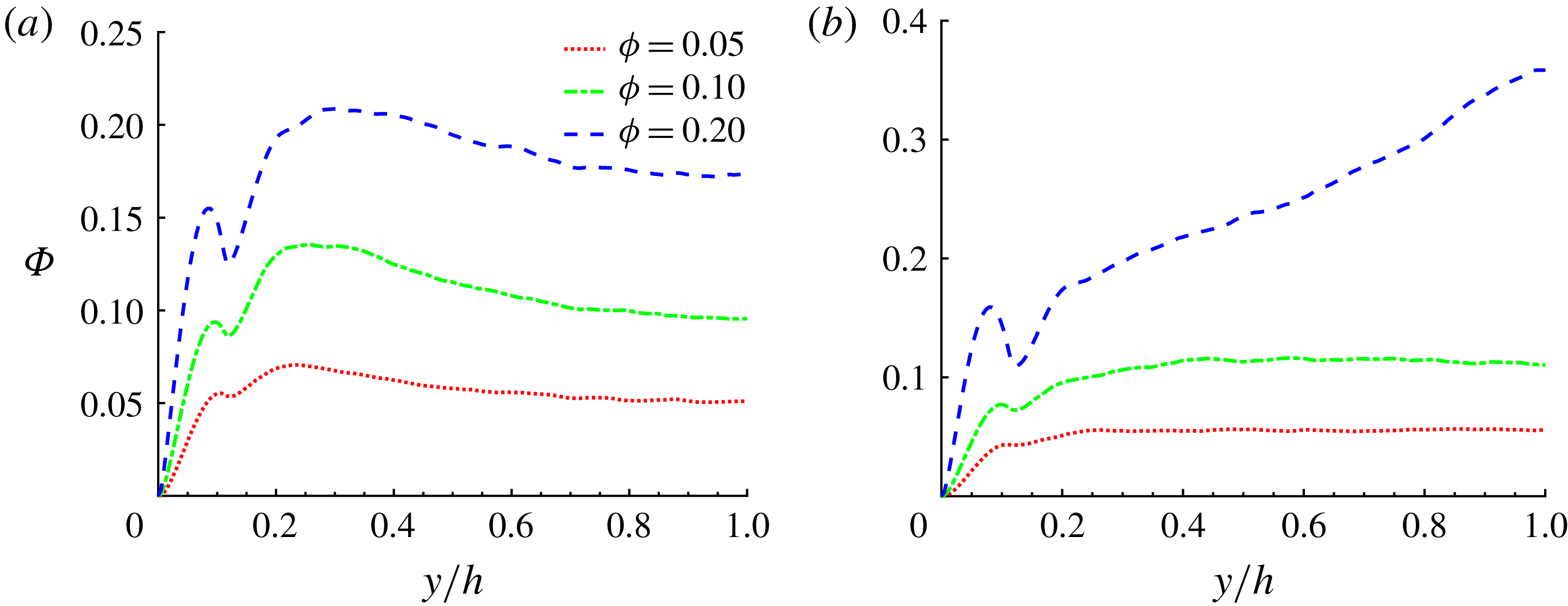
The mean particle concentration over the duct cross-section
 $\unicode[STIX]{x1D6F7}(y,z)$
is displayed in figure 6 for all
 $\unicode[STIX]{x1D719}$
, whereas the particle concentration along the wall bisector (
 $z/h=1$
) and along a segment at
 $z/h=0.2$
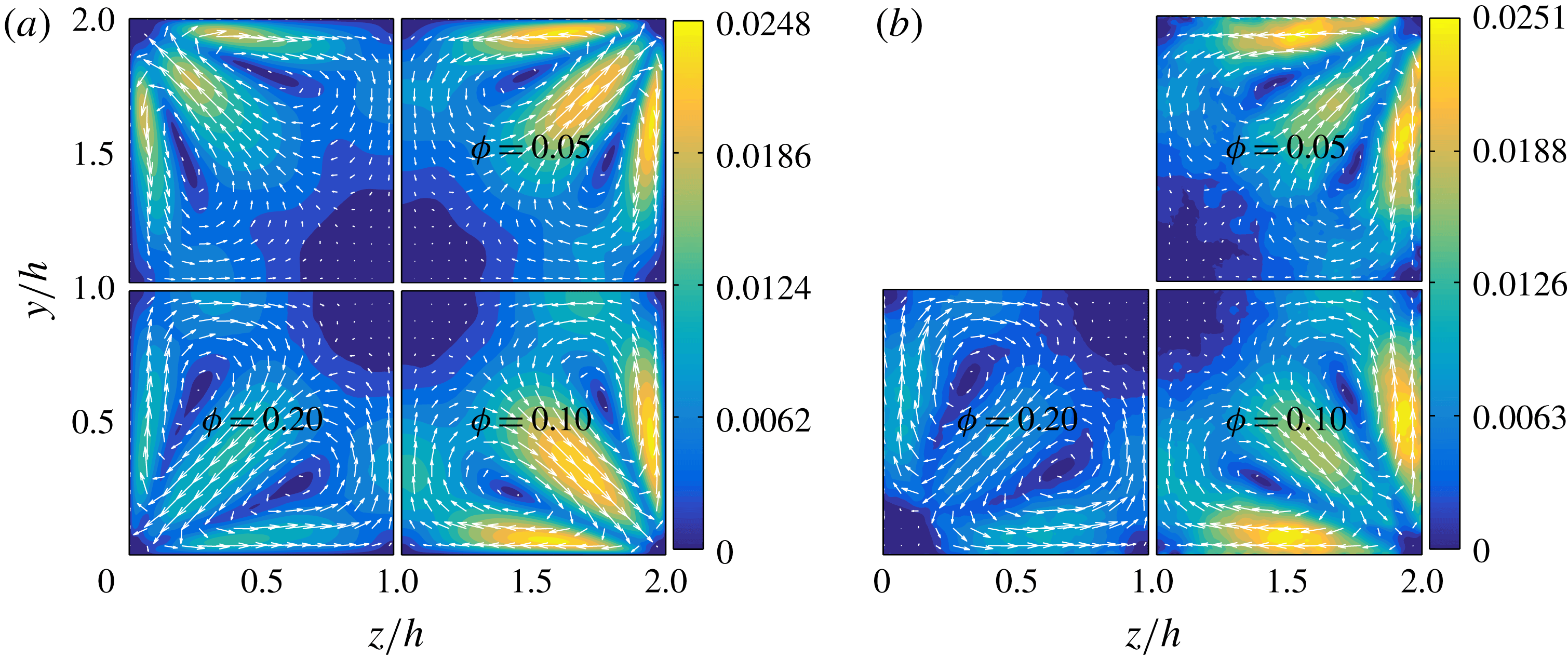
is shown in figure 7. Finally, we report in figure 8 the secondary (cross-stream) velocities of both phases, defined as
 $\sqrt{V_{f/p}^{2}+W_{f/p}^{2}}$
. We shall now discuss these three figures together.
The particle concentration distribution is defined as
 $$\begin{eqnarray}\displaystyle \unicode[STIX]{x1D6F7}(y,z)=\frac{1}{N_{t}N_{x}}\mathop{\sum }_{m=1}^{N_{t}}\mathop{\sum }_{i=1}^{N_{x}}\unicode[STIX]{x1D713}(x_{ijk},t^{m}), & & \displaystyle\end{eqnarray}$$
where
 $N_{t}$
is the number of time steps considered for the average,
 $t^{m}$
is the sampling time and
 $\unicode[STIX]{x1D713}(x_{ijk},t^{m})$
is the particle indicator function at the location
 $x_{ijk}$
and time
 $t^{m}$
. The particle indicator function is equal to 1 for points
 $x_{ijk}$
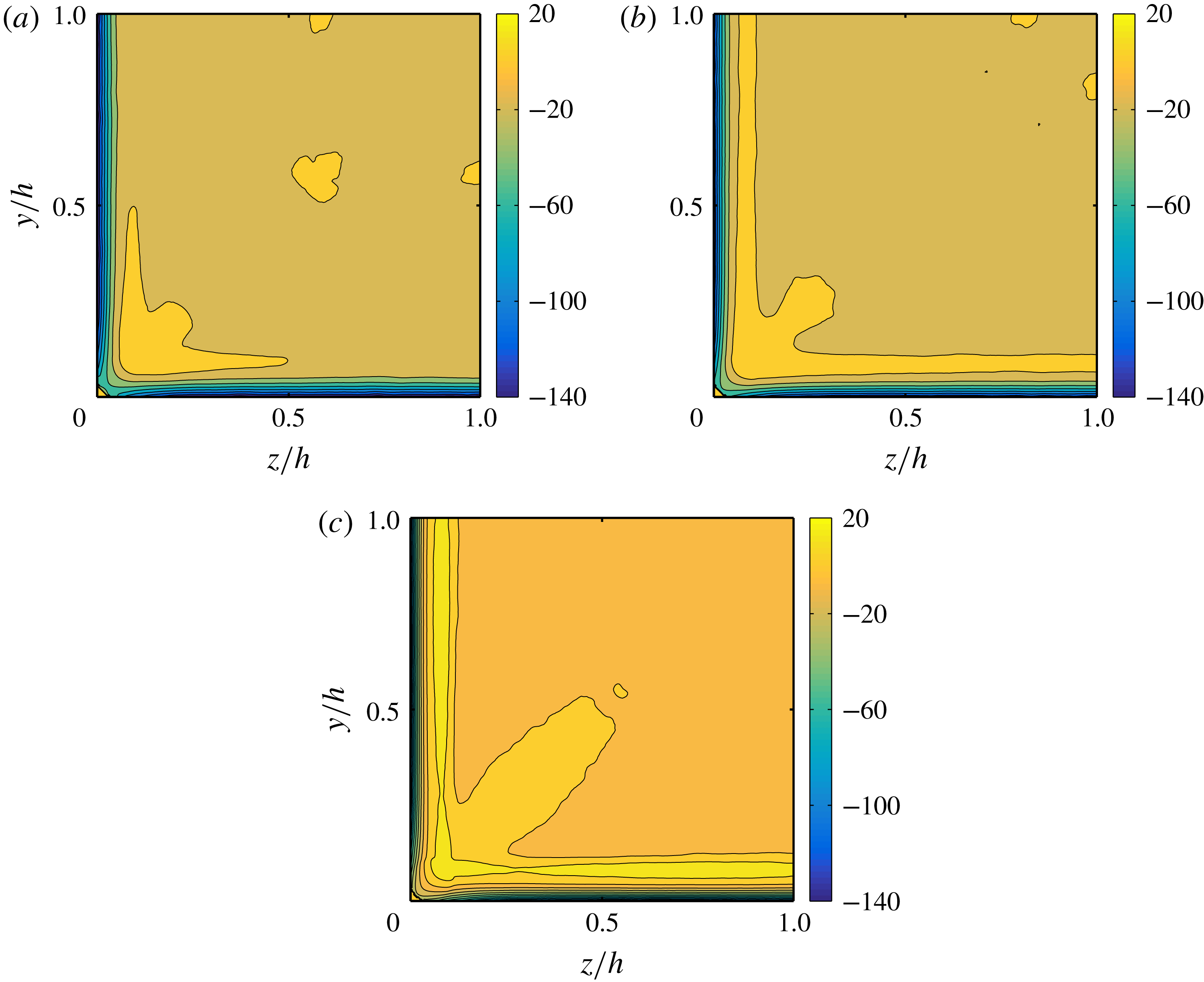
contained within the volume of a sphere, and 0 otherwise. Two interesting observations are deduced from figure 6: (i) particle layers form close to the walls, and (ii) for
 $\unicode[STIX]{x1D719}=0.05$
and 0.1, the local particle concentration
 $\unicode[STIX]{x1D6F7}(y,z)$
is higher close to the duct corners. We have recently reported a similar result for laminar duct flow at
 $Re_{b}=550$
and the same duct-to-particle size ratio,
 $h/a=18$
, and volume fractions,
 $\unicode[STIX]{x1D719}$
(Kazerooni et al.
Reference Kazerooni, Fornari, Hussong and Brandt2017). At those
 $Re_{b}$
and
 $h/a$
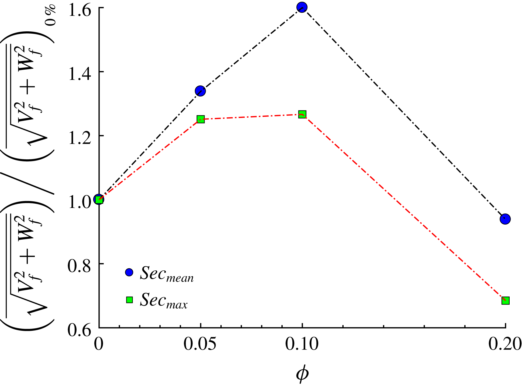
, particles undergo an inertial migration towards the walls and especially towards the corners, while the duct core is fully depleted of particles. Clearly, turbulence enhances mixing and the depletion of particles at the duct core disappears. It is also interesting to observe that the presence of particles further enhances the fluid secondary flow around the corners for
 $\unicode[STIX]{x1D719}\leqslant 0.1$
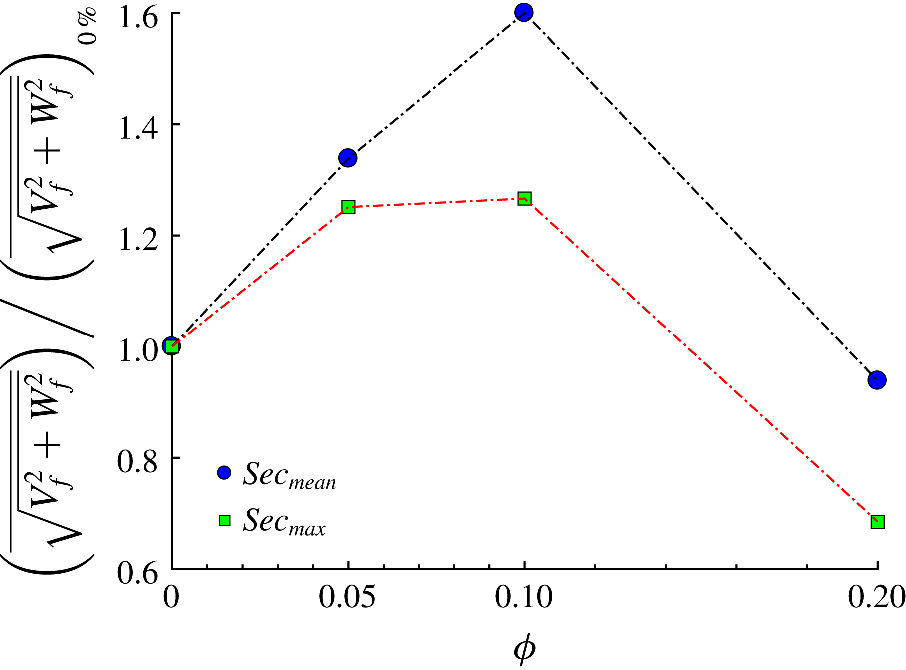
. This can be easily seen from figure 9, where both the maximum and the mean value of the secondary fluid velocity are shown as a function of the volume fraction
 $\unicode[STIX]{x1D719}$
. The maximum value of the secondary cross-stream velocity increases from approximately 2 to 2.5 % of
 $U_{b}$
. The relative increase of the mean
 $\sqrt{V_{f}^{2}+W_{f}^{2}}$
in comparison to the unladen case, is even larger than the increase in the maximum value at equal
 $\unicode[STIX]{x1D719}$
. Similarly, in laminar ducts, as particles migrate towards the corners, secondary flows are generated.
Mean particle concentration along a line at
 $z/h=0.2$
and at the wall bisector,
 $z/h=1$
.
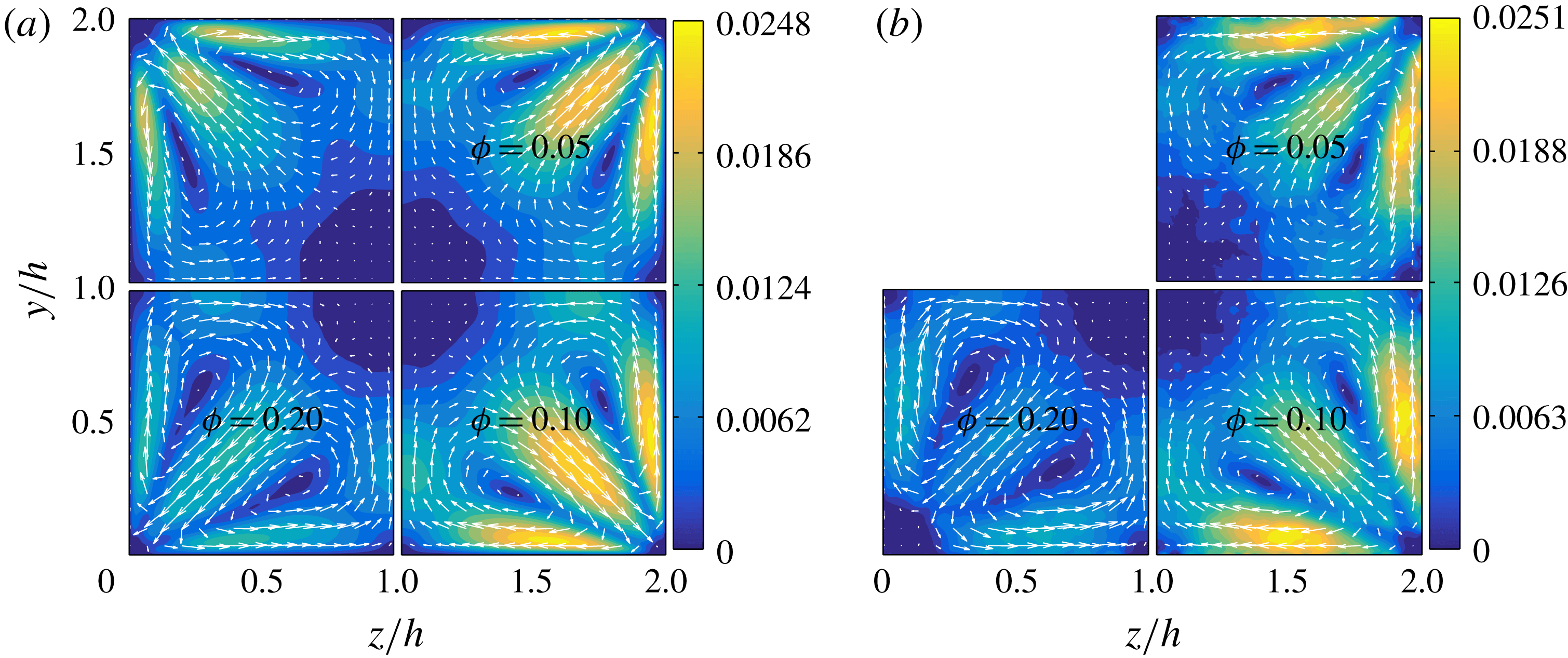
Contours and vector fields of the secondary flow velocity
 $\sqrt{V_{f/p}^{2}+W_{f/p}^{2}}$
of the fluid (a) and solid phases (b).
Mean and maximum value of the secondary flow velocity of the fluid phase as a function of the solid volume fraction
 $\unicode[STIX]{x1D719}$
. Results are normalized by the values of the single-phase case.
As shown in figure 6, the particle concentration close to the corners increases with the volume fraction. However, the mean particle distribution in the cross-section changes at the highest volume fraction considered,
 $\unicode[STIX]{x1D719}=0.2$
: the highest values of
 $\unicode[STIX]{x1D6F7}(y,z)$
are now found at the centre of the duct (see figure 7
b). This is not the case in turbulent channel flows and hence it can be related to the additional confinement of the suspension given by the lateral walls. As previously mentioned, the streamwise mean fluid and particle velocities are also substantially higher at the duct centre for
 $\unicode[STIX]{x1D719}=0.2$
.
To better quantify this effect, we analyse the numerical data by Picano et al. (Reference Picano, Breugem and Brandt2015) and calculate the number of particles crossing the spanwise periodic boundaries per unit time
 $h/U_{b}$
. For
 $\unicode[STIX]{x1D719}=20\,\%$
, we find that in 1 unit of
 $h/U_{b}$
approximately 1 % of the total number of particles cross the lateral boundaries. Inhibiting this lateral migration with lateral walls has therefore important consequences on the flow structure.
Concerning the secondary fluid velocity (figure 8
a), we note that for
 $\unicode[STIX]{x1D719}=0.2$
both the maximum and the mean values decrease below those of the unladen case. The presence of the solid phase leads to an increase of the secondary fluid velocity, which however saturates for volume fractions between 0.1 and 0.2. As shown by these mean velocity profiles, the turbulence activity is substantially reduced at
 $\unicode[STIX]{x1D719}=0.2$
.
Vector and contour plots of the secondary motions of the solid phase are reported in figure 8(b). These closely resemble those of the fluid phase. However, the velocities at the corner bisectors are almost half of those pertaining the fluid phase (in agreement with the fact that the particle concentration is high at these locations). Indeed, as discussed above there is a high particle concentration along the diagonals; particles reside for long times on these bisectors and, as a consequence they have lower cross-stream velocities than the fluid. Conversely, the cross-stream particle velocity is similar to that of the fluid phase at the walls, away from the corners. For
 $\unicode[STIX]{x1D719}=0.2$
we have previously noticed that along the duct walls, the highest particle concentration
 $\unicode[STIX]{x1D6F7}(y,z)$
is exactly at the corners. In agreement, we also observe from figure 8(b) that the secondary particle velocity is negligible at these locations (i.e. particles tend to stay at these locations for long times).
3.3 Velocity fluctuations
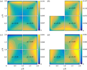
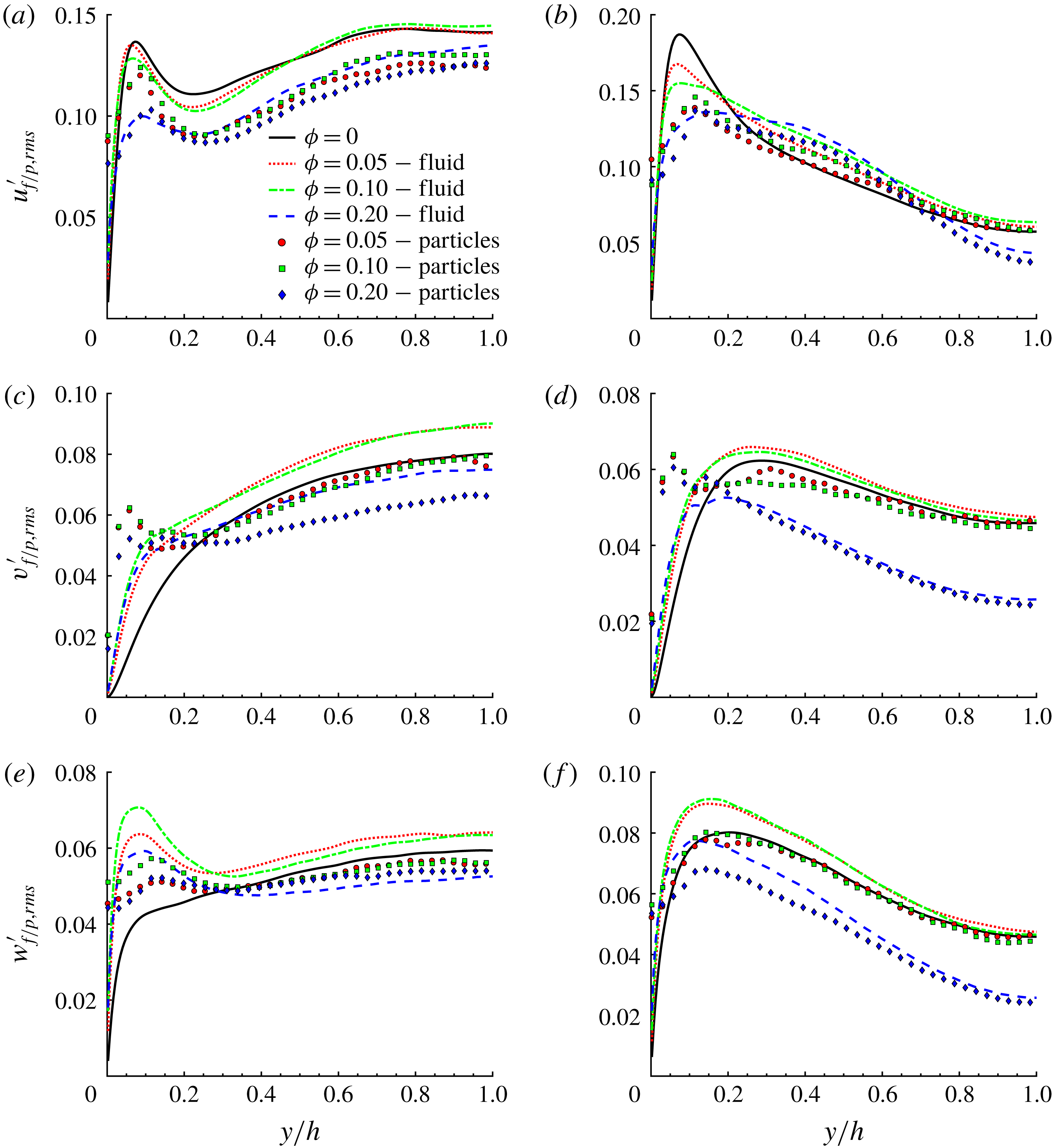
Next, we report the contours of the root-mean-square (r.m.s.) of the fluid and particle velocity fluctuations in outer units, see figure 10. Due to the symmetry around the corner bisectors, we show only the contours of
 $v_{f/p,rms}^{\prime }(y,z)$
in panels (c) and (d). Corresponding r.m.s. velocities along two lines at
 $z/h=0.2$
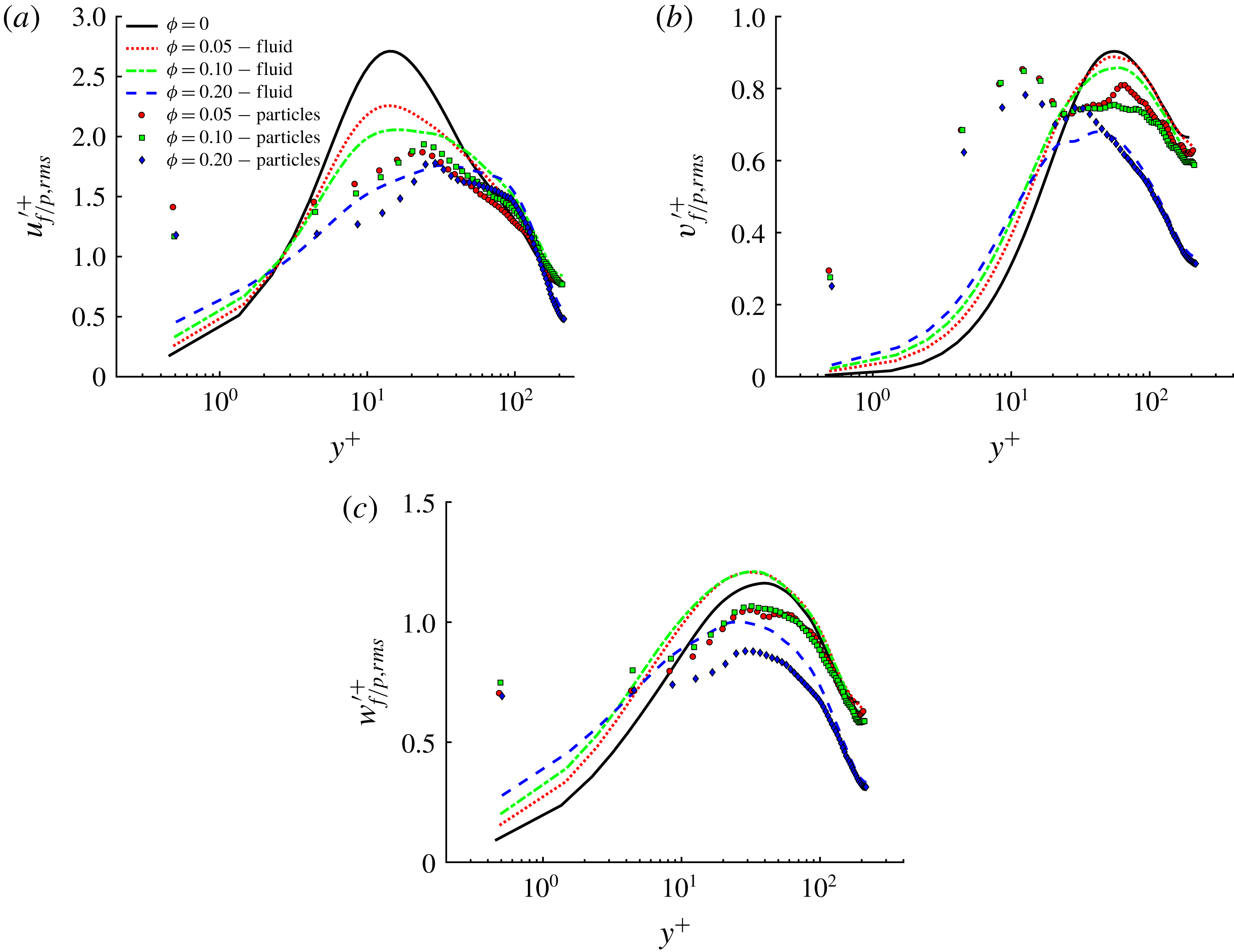
and 1 are depicted in figure 11. Results in inner units are shown at the wall bisector,
 $z/h=1$
in figure 12.
(a) Root-mean-square of the streamwise fluid velocity fluctuations in outer units,
 $u_{f,rms}^{\prime }$
, for all
 $\unicode[STIX]{x1D719}$
. (b) Root-mean-square of the streamwise particle velocity fluctuations in outer units,
 $u_{p,rms}^{\prime }$
, for all
 $\unicode[STIX]{x1D719}$
. (c) Root-mean-square of the vertical fluid velocity fluctuations in outer units,
 $v_{f,rms}^{\prime }$
, for all
 $\unicode[STIX]{x1D719}$
. (d) Root-mean-square of the vertical particle velocity fluctuations in outer units
 $v_{p,rms}^{\prime }$
, for all
 $\unicode[STIX]{x1D719}$
.
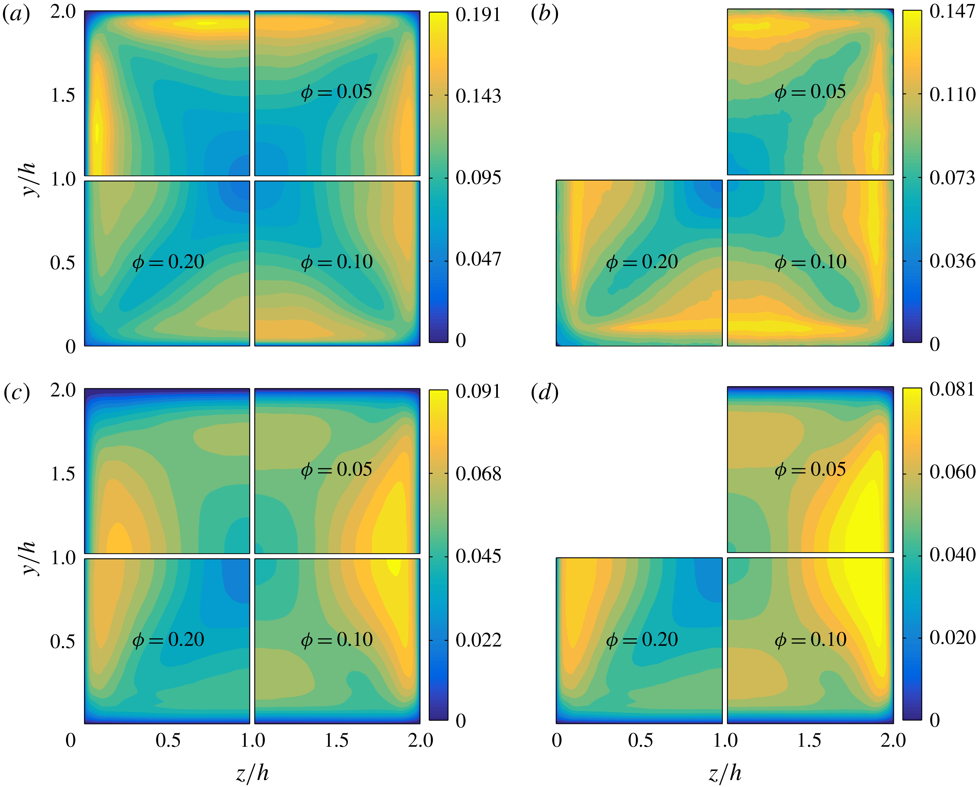
The contours of the streamwise fluid velocity fluctuations reveal that r.m.s. values are stronger near the walls (close to the wall bisector), while minima are found along the corner bisectors. In this region,
 $u_{f,rms}^{\prime }(y,z)$
is substantially reduced for
 $\unicode[STIX]{x1D719}=0.2$
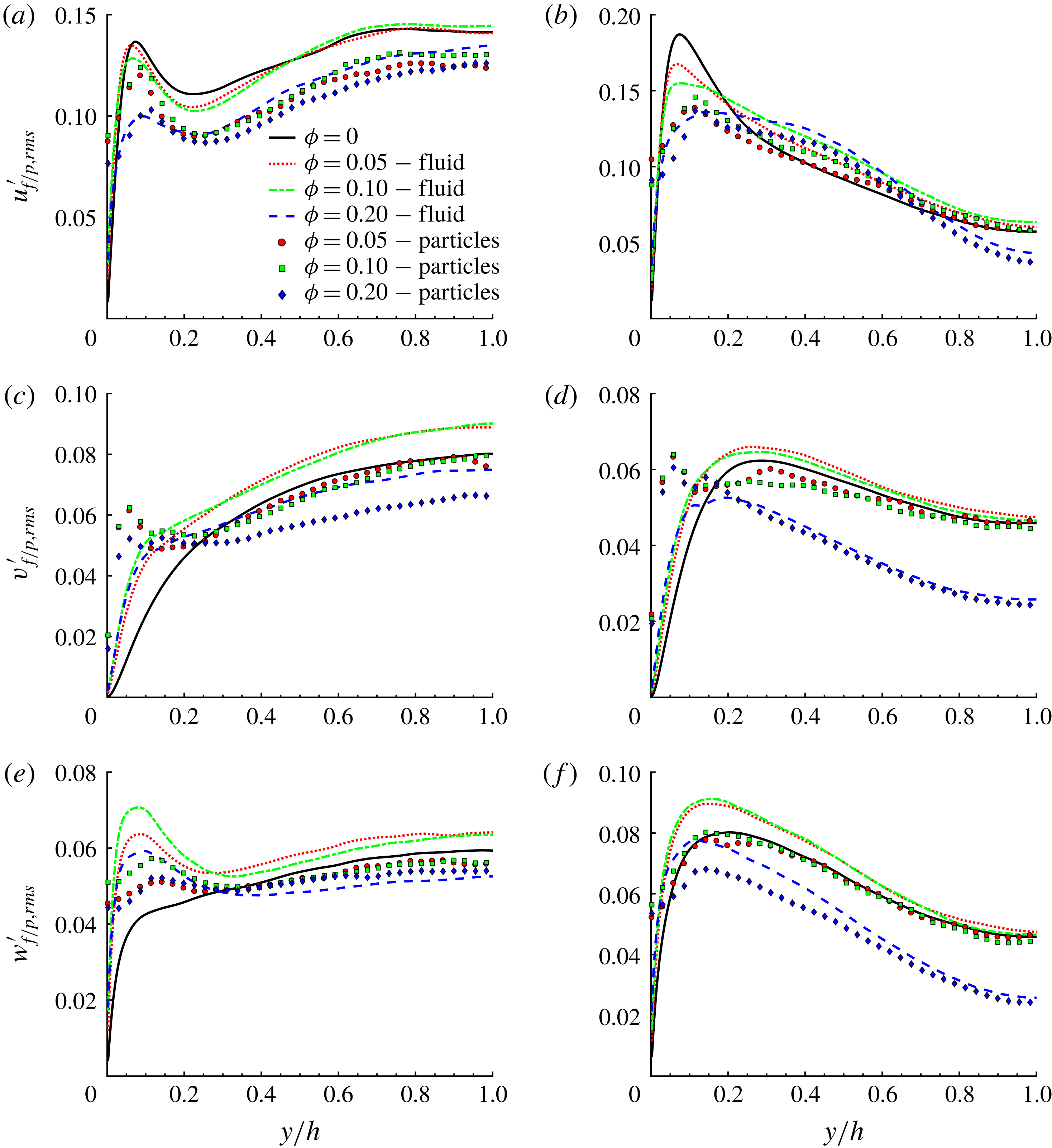
, as also visible from the profiles in figure 11(a). From figure 11(a) we also see that the local maxima of
 $u_{f,rms}^{\prime }(y)$
close to the corners is of similar magnitude for
 $\unicode[STIX]{x1D719}=0.0,0.05$
and 0.1. On the other hand, at the wall bisectors the maxima of
 $u_{f,rms}^{\prime }(y,z)$
decrease with
 $\unicode[STIX]{x1D719}$
, well below the value of the unladen case (see figure 11
b). For
 $\unicode[STIX]{x1D719}=0.2$
the profile of
 $u_{f,rms}^{\prime }(y)$
deeply changes. In particular, the streamwise r.m.s. velocity
 $u_{f,rms}^{\prime }(y)$
is substantially smaller than in the unladen case in the core region, where the particle concentration and the mean velocity are high while the secondary flows are negligible. After the maximum value,
 $u_{f,rms}^{\prime }(y)$
initially decreases smoothly and then sharply for
 $y/h>0.6$
.
From figures 10(b) and 11(a,b) we see that the streamwise r.m.s. particle velocity,
 $u_{p,rms}^{\prime }(y,z)$
, resembles that of the fluid phase. However,
 $u_{p,rms}^{\prime }(y,z)$
is typically smaller than
 $u_{f,rms}^{\prime }(y,z)$
in the cross-section. Exceptions are the regions close to the walls where the particle velocity does not vanish (unlike the fluid velocity).
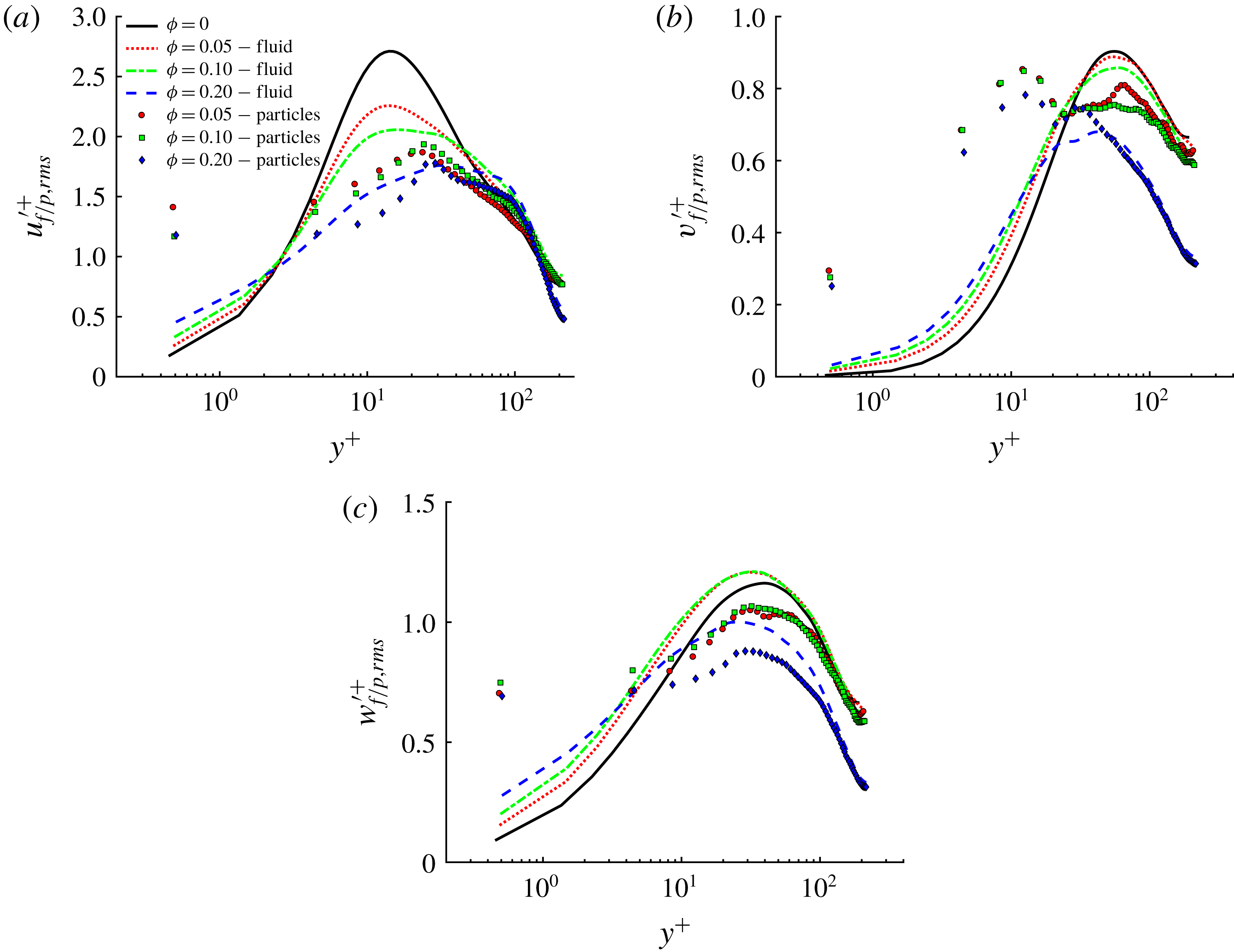
Root-mean-square of fluid and particle velocity fluctuations: (a,b) streamwise, (c,d) wall-normal and (e,f) spanwise (
 $z$
-direction) components in outer units at
 $z/h=0.2$
(a,c,e) and
 $z/h=1$
(b,d,f), for all
 $\unicode[STIX]{x1D719}$
. Lines and symbols are used for the fluid and solid phase statistics, respectively.
From the contour of
 $v_{f,rms}^{\prime }(y,z)$
(see figure 10
c), we see that r.m.s. velocities are larger in the directions parallel to the walls, rather than in the wall-normal direction. Close to the wall bisectors, the peak values of the wall-normal and parallel fluid r.m.s. velocities increase with
 $\unicode[STIX]{x1D719}$
, again except for
 $\unicode[STIX]{x1D719}=0.2$
when turbulence is damped. From figure 11(c,e) we see instead that close to the corners, the local maxima of both
 $v_{f,rms}^{\prime }(y)$
(wall normal) and
 $w_{f,rms}^{\prime }(y)$
(wall parallel) increase with respect to the unladen case, for all
 $\unicode[STIX]{x1D719}$
. At the wall bisector (see figure 11
d), wall-normal velocity fluctuations are slightly larger than the single-phase case for
 $\unicode[STIX]{x1D719}\lesssim 0.1$
.
Finally, figure 11(f) shows profiles at the wall bisector of the parallel component of the fluid velocity r.m.s.,
 $w_{f,rms}^{\prime }(y)$
. Note that the peak value of
 $w_{f,rms}^{\prime }(y)$
increases with the volume fraction up to
 $\unicode[STIX]{x1D719}=0.1$
and moves closer to the wall. There is hence a clear redistribution of energy due to the particle presence towards a slightly more isotropic state.
Root-mean-square of fluid and particle velocity fluctuations: (a) streamwise, (b) wall-normal and (c) spanwise (
 $z$
-)direction components in inner units at
 $z/h=1$
for all
 $\unicode[STIX]{x1D719}$
. Lines and symbols are used for the fluid- and solid-phase statistics as in figure 11.
Concerning the solid phase, the wall-normal particle r.m.s. velocity,
 $v_{p,rms}^{\prime }$
, exhibits a peak close to the walls where particle layers form, see figures 10(d) and 11(d) (and also Costa et al.
Reference Costa, Picano, Brandt and Breugem2016). Differently from the channel flow analysed by Picano et al. (Reference Picano, Breugem and Brandt2015), in the square duct flow
 $v_{p,rms}^{\prime }$
decreases slowly with increasing volume fraction
 $\unicode[STIX]{x1D719}$
in the wall particle layer (
 $y^{+}\leqslant 20$
) and the maxima are similar for all
 $\unicode[STIX]{x1D719}$
. This may be related to the existence of the secondary flows that pull the particles away from the walls towards the duct core. As for the fluid phase, the particle r.m.s. velocity parallel to the wall is greater than the perpendicular component close to the walls. From the profiles at the wall bisector, see figure 11(f), we also see that the maximum of
 $w_{p,rms}^{\prime }(y)$
is similar for
 $\unicode[STIX]{x1D719}=0.05$
and 0.1, while it clearly decreases for the densest case simulated. More generally, we observe that particle r.m.s. velocities are similar to those of the fluid phase towards the core of the duct.
Both fluid- and solid-phase r.m.s. velocities are shown in inner units at the wall bisector in figure 12(a–c). The local friction velocity has been used to normalize the velocity fluctuations. The fluid-phase r.m.s. velocity increases with
 $\unicode[STIX]{x1D719}$
in the viscous sublayer. Clearly, the presence of solid particles introduces additional disturbances in the fluid increasing the level of fluctuations in regions where these are typically low (in the unladen case). On the other hand, particle velocity fluctuations are typically smaller than the corresponding fluid r.m.s. velocity, except in the inner-wall region,
 $y^{+}<20$
, where they are one order of magnitude larger.
Mean turbulence intensity
 $I=\langle u^{\prime }\rangle /U_{b}$
for all
 $\unicode[STIX]{x1D719}$
, normalized by the value for the unladen case.
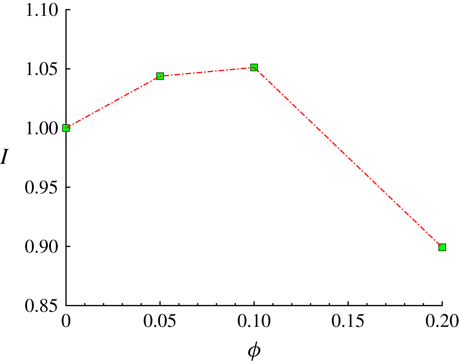
Finally, we also computed the mean turbulence intensity defined as
 $I=\langle u^{\prime }\rangle /U_{b}$
, with
 $u^{\prime }=\sqrt{1/3(u_{f,rms}^{\prime 2}+v_{f,rms}^{\prime 2}+w_{f,rms}^{\prime 2})}$
. This is shown is figure 13, where results are normalized by the value obtained for the unladen case. As for secondary flows, we see that the turbulence intensity
 $I$
increases up to
 $\unicode[STIX]{x1D719}=0.1$
, for which
 $I$
is approximately 5 % larger than the unladen value. For
 $\unicode[STIX]{x1D719}=0.2$
, instead, the mean turbulence intensity decreases well below the single-phase value, and
 $I(\unicode[STIX]{x1D719}=0.2)\sim 0.9\,I(\unicode[STIX]{x1D719}=0)$
. It can be expected that when the volume fraction is larger than a threshold value (
 $0.1<\unicode[STIX]{x1D719}\leqslant 0.2$
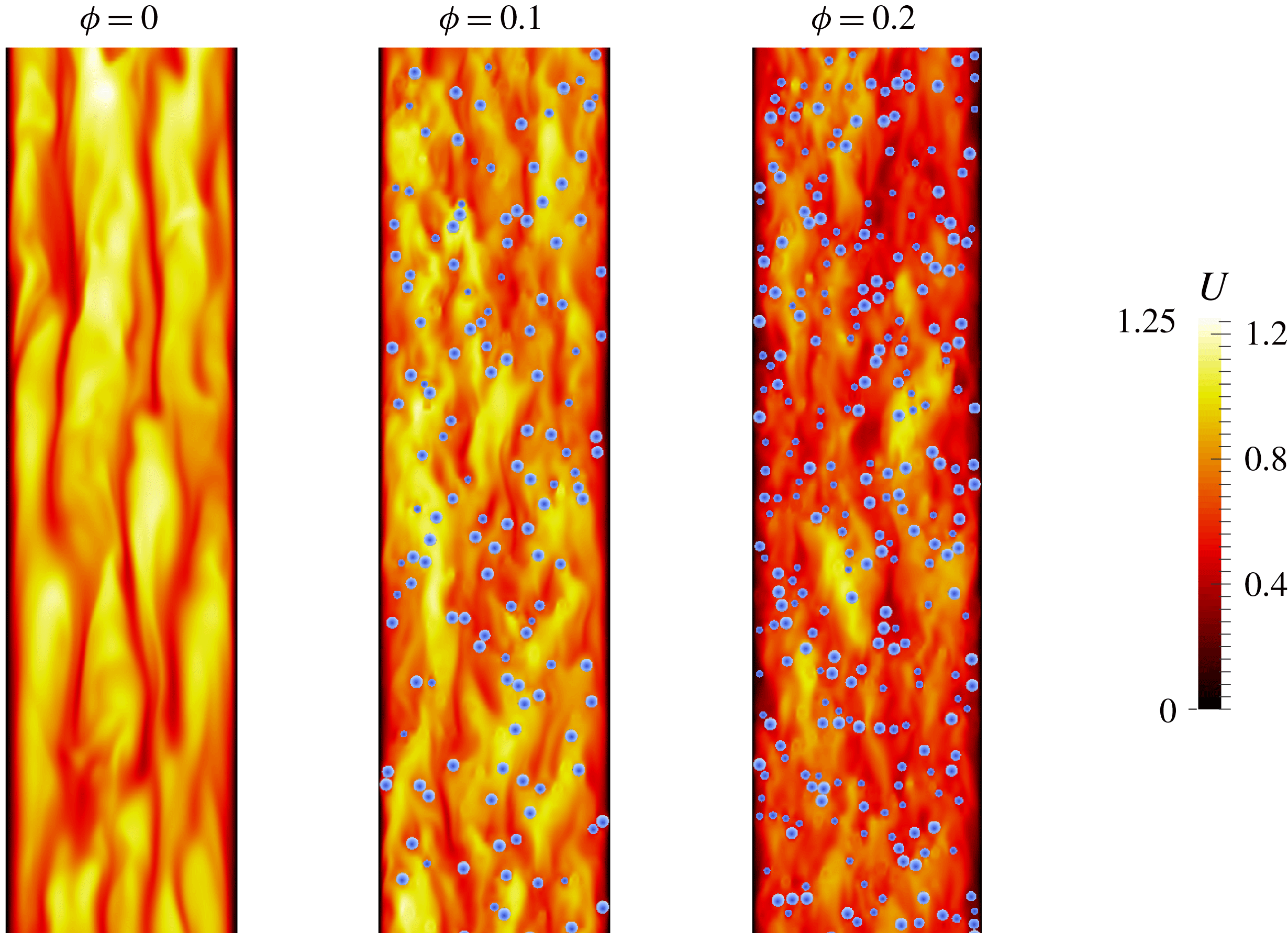
), the particles are almost closely packed in the near-wall region. As a consequence, the quasi-coherent turbulent structures are quickly disrupted (as can be seen in figure 14) and the turbulence regenerating cycle is modified. As we will see in the next section, there is a strong reduction of the primary Reynolds stresses at
 $\unicode[STIX]{x1D719}=0.2$
, especially in the regions close to the wall bisector. Since the mean fluid velocity gradients are also reduced in the near-wall region with respect to
 $\unicode[STIX]{x1D719}=0.1$
, it can be expected that the associated turbulence production (
 $\langle u_{f}^{\prime }v_{f}^{\prime }\rangle \text{d}U_{f}/\text{d}y+\langle u_{f}^{\prime }w_{f}^{\prime }\rangle \text{d}U_{f}/\text{d}z$
) will be strongly reduced, leading to the observed reduction in turbulence intensity.
In addition, we also calculated the fraction of the global kinetic energy that is contained in each phase, and the overall energy dissipation (per unit density) of the fluid phase,
 $\unicode[STIX]{x1D716}_{T}=2\unicode[STIX]{x1D707}\langle \unicode[STIX]{x1D60C}_{ij}\unicode[STIX]{x1D60C}_{ij}\rangle$
, averaged over time and volume, and normalized by
 $\unicode[STIX]{x1D708}U_{b}^{2}/(2h)^{2}$
(
 $\unicode[STIX]{x1D60C}_{ij}=0.5(\unicode[STIX]{x2202}u_{i}/\unicode[STIX]{x2202}x_{j}+\unicode[STIX]{x2202}u_{j}/\unicode[STIX]{x2202}x_{i})$
is the strain-rate tensor). The global kinetic energy is defined as
 $K=K_{f}+K_{p}=0.5(U_{f,i}^{2}+u_{f,rms,i}^{\prime 2})+0.5(U_{p,i}^{2}+u_{p,rms,i}^{\prime 2})$
, where
 $K_{f}$
and
 $K_{p}$
are the total energies of the fluid and solid phase. We find that 6 %, 12 % and 24 % of
 $K$
is contained in the particle phase for
 $\unicode[STIX]{x1D719}=0.05,0.1$
and 0.2. Clearly, these values are proportional to the solid volume fraction.
Concerning the mean values of the overall energy dissipation, we see that they increase with the volume fraction, up to
 $\unicode[STIX]{x1D719}=0.1$
. In particular,
 $\unicode[STIX]{x1D716}_{T}=23,28$
and 30 for
 $\unicode[STIX]{x1D719}=0.0,0.05$
and 0.1. Instead, for
 $\unicode[STIX]{x1D719}=0.2$
,
 $\unicode[STIX]{x1D716}_{T}=28$
. Generally, a reduction in
 $\unicode[STIX]{x1D716}_{T}$
is related to turbulence attenuation as discussed, for example, by Spandan, Lohse & Verzicco (Reference Spandan, Lohse and Verzicco2016). As shown in figure 14, it is difficult to identify quasi-coherent structures at
 $\unicode[STIX]{x1D719}=0.2$
(due to the large number of particles near the walls), and as we will later explain, ejection events that are typically (very) intense close to the wall bisectors, substantially reduce in this case. The turbulence activity is hence reduced as shown by the reduction in energy dissipation, turbulence intensity and, as we will discuss in the next sections, of the primary Reynolds stresses and mean streamwise vorticity.
At
 $\unicode[STIX]{x1D719}=0.2$
, the stronger reduction in turbulence activity in comparison to channel flow may be due to the geometrical constraint given by the lateral walls. From the data of Picano et al. (Reference Picano, Breugem and Brandt2015), it can be found that on average 7.5 % of the particles reside near the walls (between
 $y/h=0$
and
 $y/h\sim 0.12$
). In duct flow instead, we find that 13.1 % of the particles are located close to one of the 4 walls. There are hence almost twice as many particles interacting with the near-wall turbulence, leading to its stronger attenuation. It is also interesting to note that for all
 $\unicode[STIX]{x1D719}$
, the amount of particles located close to the walls is always approximately 13 % of the total. This observation can be relevant for modelling purposes as done by Costa et al. (Reference Costa, Picano, Brandt and Breugem2016) who divide a particle-laden turbulent flow into a near-wall particle layer and a homogeneous suspension bulk flow.
The magnitude of the fluid velocity (normalized by
 $U_{b}$
) at
 $y^{+}\simeq 20$
for
 $\unicode[STIX]{x1D719}=0.0,0.1$
and 0.2.
3.4 Reynolds stress and mean fluid streamwise vorticity
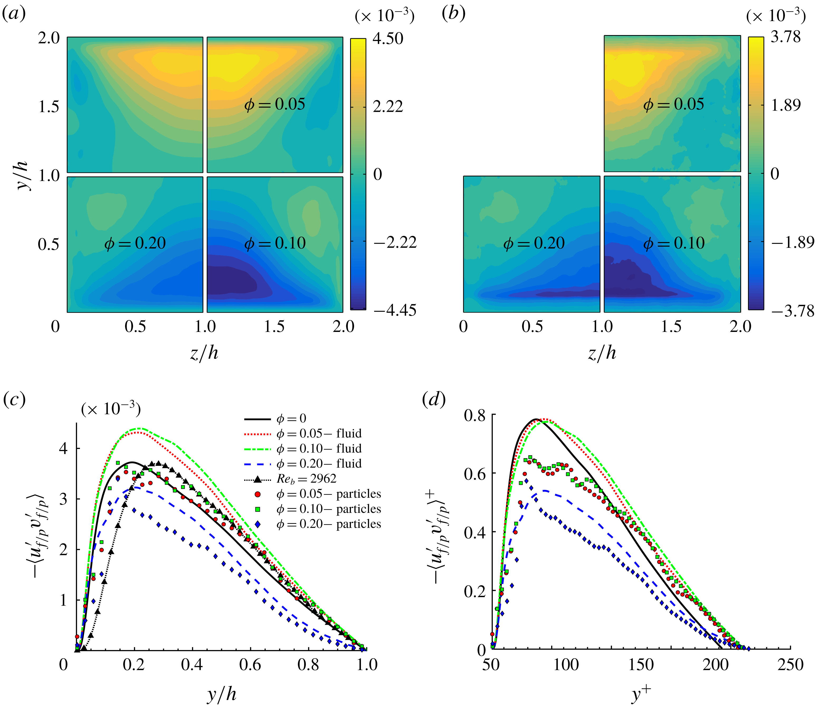
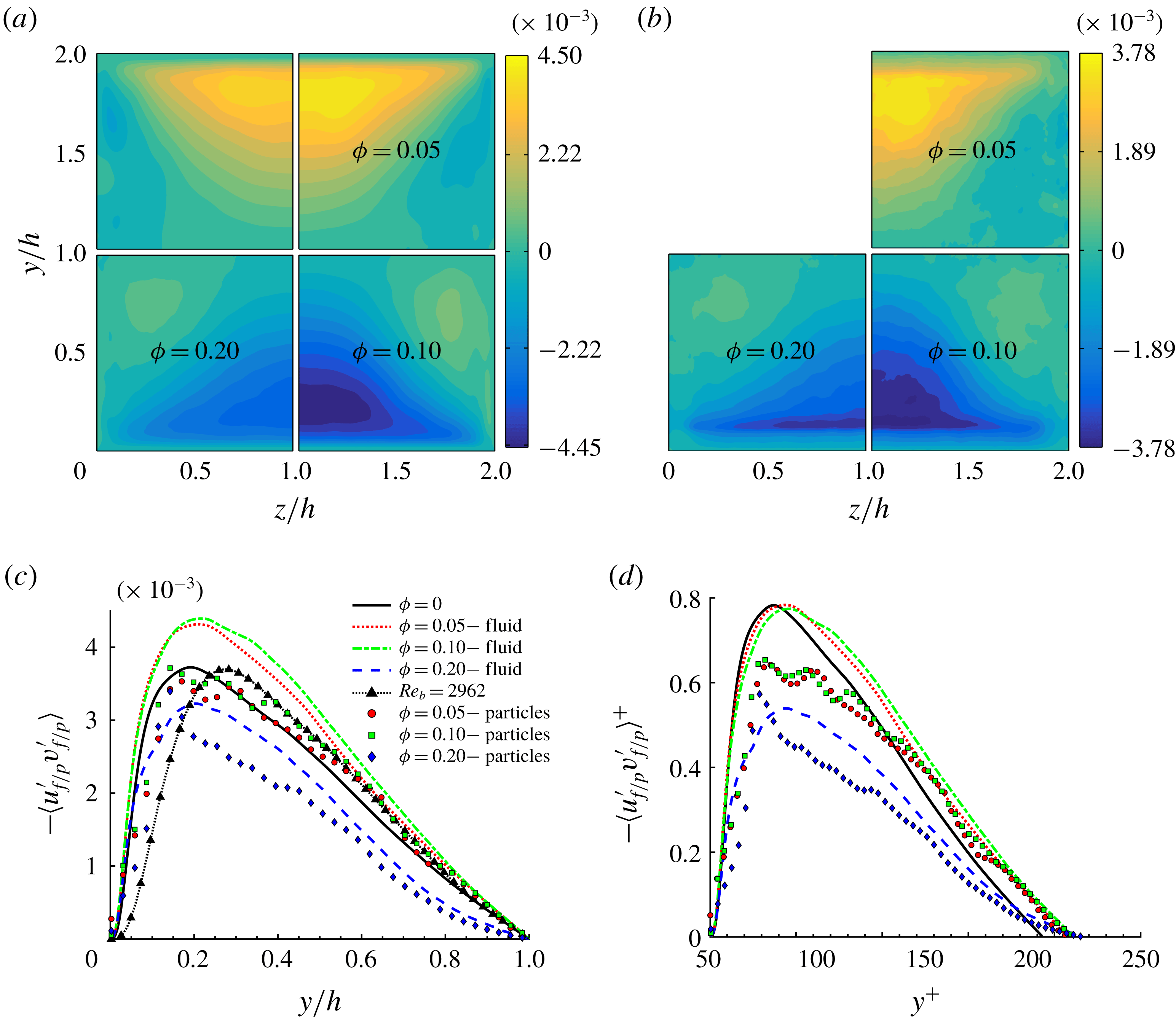
We now turn to the discussion of the primary Reynolds stress in the duct cross-section, as this plays an important role in the advection of mean streamwise momentum. We show in figure 15(a) the
 $\langle u_{f}^{\prime }v_{f}^{\prime }\rangle$
component of the fluid Reynolds stress in the duct cross-section, for all
 $\unicode[STIX]{x1D719}$
. The component
 $\langle u_{f}^{\prime }w_{f}^{\prime }\rangle$
is not shown as it is the
 $90^{\circ }$
rotation of
 $\langle u_{f}^{\prime }v_{f}^{\prime }\rangle$
. We see that the maximum of
 $\langle u_{f}^{\prime }v_{f}^{\prime }\rangle$
, located close to the wall bisector, increases with the volume fraction up to
 $\unicode[STIX]{x1D719}=0.1$
. The maximum
 $\langle u_{f}^{\prime }v_{f}^{\prime }\rangle$
then progressively decreases with
 $\unicode[STIX]{x1D719}$
, denoting a reduction in turbulent activity. For
 $\unicode[STIX]{x1D719}=0.2$
we observe that the maximum of
 $\langle u_{f}^{\prime }v_{f}^{\prime }\rangle$
reaches values even lower than in the unladen case. The contour of
 $\langle u_{f}^{\prime }v_{f}^{\prime }\rangle$
also changes with increasing
 $\unicode[STIX]{x1D719}$
. We find that
 $\langle u_{f}^{\prime }v_{f}^{\prime }\rangle$
increases towards the corners, and also for
 $\unicode[STIX]{x1D719}=0.2$
it is larger than in the unladen case. However, the mean value of
 $\langle u_{f}^{\prime }v_{f}^{\prime }\rangle$
in one quadrant slightly increases up to
 $\unicode[STIX]{x1D719}=0.1$
, while for
 $\unicode[STIX]{x1D719}=0.2$
the mean is 26 % smaller than for the unladen case.
Contours of the primary Reynolds stress
 $\langle u_{f/p}^{\prime }v_{f/p}^{\prime }\rangle$
of (a) the fluid and (b) particle phase for all volume fractions considered. The profiles along the wall bisector at
 $z/h=1$
are shown in outer and inner units in panels (c) and (d). Lines and symbols are used for the fluid- and solid-phase statistics as in figure 11.
The profiles of
 $\langle u_{f}^{\prime }v_{f}^{\prime }\rangle$
at the wall bisector (
 $z/h=1$
) are shown in figure 15(c). While the profiles for
 $\unicode[STIX]{x1D719}=0.05$
and 0.1 are similar and assume larger values than the reference case, we see that for
 $\unicode[STIX]{x1D719}=0.2$
the profile is substantially lower for all
 $z/h>0.2$
. This is also different to what is found in channel flow as close to the core,
 $\langle u_{f}^{\prime }v_{f}^{\prime }\rangle$
is found to be similar for
 $\unicode[STIX]{x1D719}=0.0$
and 0.2. This is probably related to the high particle concentration at the duct core, see figure 6(c). Looking at the profiles in inner units, see figure 15(d), we also see that the peak values of
 $\langle u_{f}^{\prime }v_{f}^{\prime }\rangle ^{+}$
are similar for the unladen case and for the laden cases with
 $\unicode[STIX]{x1D719}=0.05$
and 0.1. This is in contrast to what is found in channel flows, where a reduction of the peak with
 $\unicode[STIX]{x1D719}$
is observed (Picano et al.
Reference Picano, Breugem and Brandt2015). This shows that up to
 $\unicode[STIX]{x1D719}=0.1$
, the turbulence activity is not significantly reduced by the presence of particles. On the other hand, for
 $\unicode[STIX]{x1D719}=0.2$
we observe a large reduction in the maximum
 $\langle u_{f}^{\prime }v_{f}^{\prime }\rangle ^{+}$
, denoting an important reduction in turbulent activity.
The Reynolds stress of the solid phase,
 $\langle u_{p}^{\prime }v_{p}^{\prime }\rangle$
, is also shown for comparison in figure 15(b–d). The profiles are similar to those of the fluid phase, although
 $\langle u_{p}^{\prime }v_{p}^{\prime }\rangle <\langle u_{f}^{\prime }v_{f}^{\prime }\rangle$
for all
 $\unicode[STIX]{x1D719}$
, except close to the walls for
 $\unicode[STIX]{x1D719}=0.2$
. These local maxima may be related to the higher local particle concentration in layers close to the walls.
In figure 15(c) we also show the profile of
 $\langle u_{f}^{\prime }v_{f}^{\prime }\rangle$
obtained from an additional simulation. Here, we have used the Eilers fit (Stickel & Powell Reference Stickel and Powell2005) to estimate the effective viscosity of the suspension at
 $\unicode[STIX]{x1D719}=0.2$
and found
 $\unicode[STIX]{x1D708}_{e}/\unicode[STIX]{x1D708}=[1+2.5\unicode[STIX]{x1D719}/(1-\unicode[STIX]{x1D719}/0.6)]^{2}=1.89$
. With this value we can define an effective bulk Reynolds number,
 $Re_{e}=Re_{b}\unicode[STIX]{x1D708}/\unicode[STIX]{x1D708}_{e}=2962$
, ideally the bulk Reynolds number of a suspension of uniformly distributed monodispersed spheres. The results of a new unladen simulation with
 $Re_{b}=Re_{e}=2962$
are compared in figure 15(c) with those of the case with
 $\unicode[STIX]{x1D719}=0.2$
. We see that for
 $\unicode[STIX]{x1D719}=0.2$
, the maximum of
 $\langle u_{f}^{\prime }v_{f}^{\prime }\rangle$
is lower than that in the simulation with
 $Re_{e}=2962$
. This indicates that the turbulence attenuation is larger than what can be expected by just modelling the suspension rheological properties (i.e.
 $\unicode[STIX]{x1D708}_{e}/\unicode[STIX]{x1D708}$
). Therefore the specific size of the particles (
 ${\sim}20^{+}$
units), and their high concentration at the walls (13.1 % of
 $N_{p}$
) contribute strongly to the turbulence attenuation. This clearly shows, that the effects of a non-uniform particle distribution should be considered when trying to model such flows.
While for turbulent channel flow the cross-stream component of the Reynolds stress tensor,
 $\langle v_{f}^{\prime }w_{f}^{\prime }\rangle$
, is identically zero, in duct flow it is finite and contributes to the production or dissipation of mean streamwise vorticity. Hence it is directly related to the origin of mean secondary flows (Gessner Reference Gessner1973; Gavrilakis Reference Gavrilakis1992). This can be seen from the Reynolds-averaged streamwise vorticity equation for a fully developed single-phase duct flow,
 $$\begin{eqnarray}\displaystyle V_{f}\frac{\unicode[STIX]{x2202}\unicode[STIX]{x1D6FA}_{f}}{\unicode[STIX]{x2202}y}+W_{f}\frac{\unicode[STIX]{x2202}\unicode[STIX]{x1D6FA}_{f}}{\unicode[STIX]{x2202}z}+\frac{\unicode[STIX]{x2202}^{2}(\langle w_{f}^{\prime 2}\rangle -\langle v_{f}^{\prime 2}\rangle )}{\unicode[STIX]{x2202}y\unicode[STIX]{x2202}z}+\left(\frac{\unicode[STIX]{x2202}^{2}}{\unicode[STIX]{x2202}y^{2}}-\frac{\unicode[STIX]{x2202}^{2}}{\unicode[STIX]{x2202}z^{2}}\right)\langle v_{f}^{\prime }w_{f}^{\prime }\rangle -\unicode[STIX]{x1D708}\left(\frac{\unicode[STIX]{x2202}^{2}}{\unicode[STIX]{x2202}y^{2}}+\frac{\unicode[STIX]{x2202}^{2}}{\unicode[STIX]{x2202}z^{2}}\right)\unicode[STIX]{x1D6FA}_{f}=0, & & \displaystyle \nonumber\\ \displaystyle & & \displaystyle\end{eqnarray}$$
where
 $V_{f}$
and
 $W_{f}$
are the mean velocities in the two wall-normal directions, and the mean vorticity is defined as
 $$\begin{eqnarray}\displaystyle \unicode[STIX]{x1D6FA}_{f}=\frac{\unicode[STIX]{x2202}W_{f}}{\unicode[STIX]{x2202}y}-\frac{\unicode[STIX]{x2202}V_{f}}{\unicode[STIX]{x2202}z}. & & \displaystyle\end{eqnarray}$$
The first two terms of (3.4) represent the convection of mean vorticity by the secondary flow itself and have been shown to be almost negligible (Gavrilakis Reference Gavrilakis1992). The third term is a source of vorticity in the viscous sublayer due to the gradients in the anisotropy of the cross-stream normal stresses. The fourth term, involving the secondary Reynolds stress, acts as source or sink of vorticity. Finally, the last term represents the viscous diffusion of vorticity.
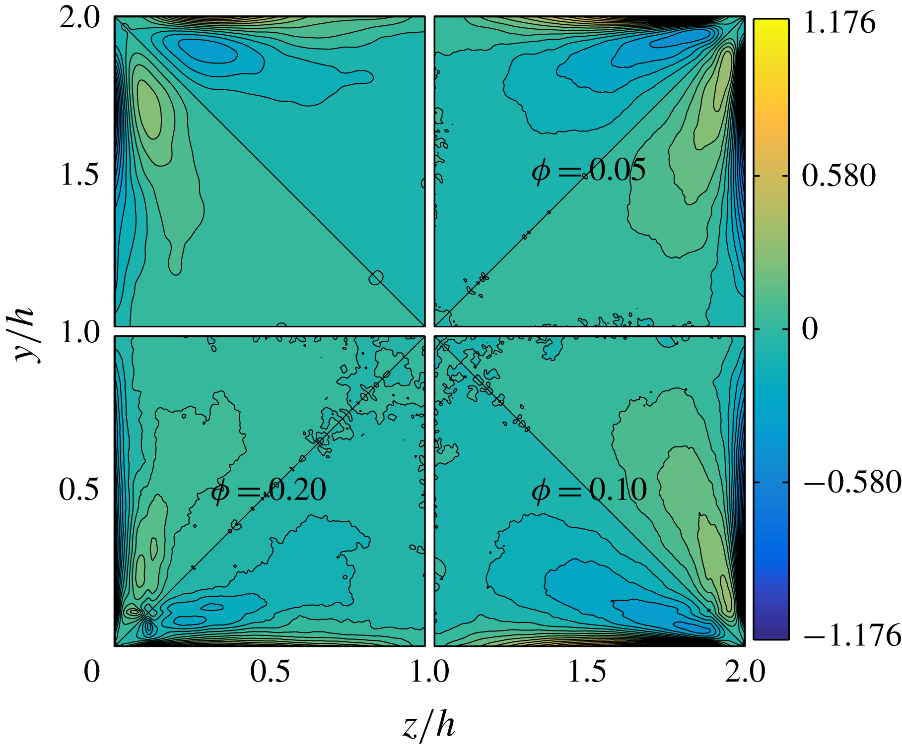
Contours of the secondary Reynolds stress
 $\langle v_{f/p}^{\prime }w_{f/p}^{\prime }\rangle$
of (a) the fluid and (b) the particle phase for all volume fractions
 $\unicode[STIX]{x1D719}$
under investigation.
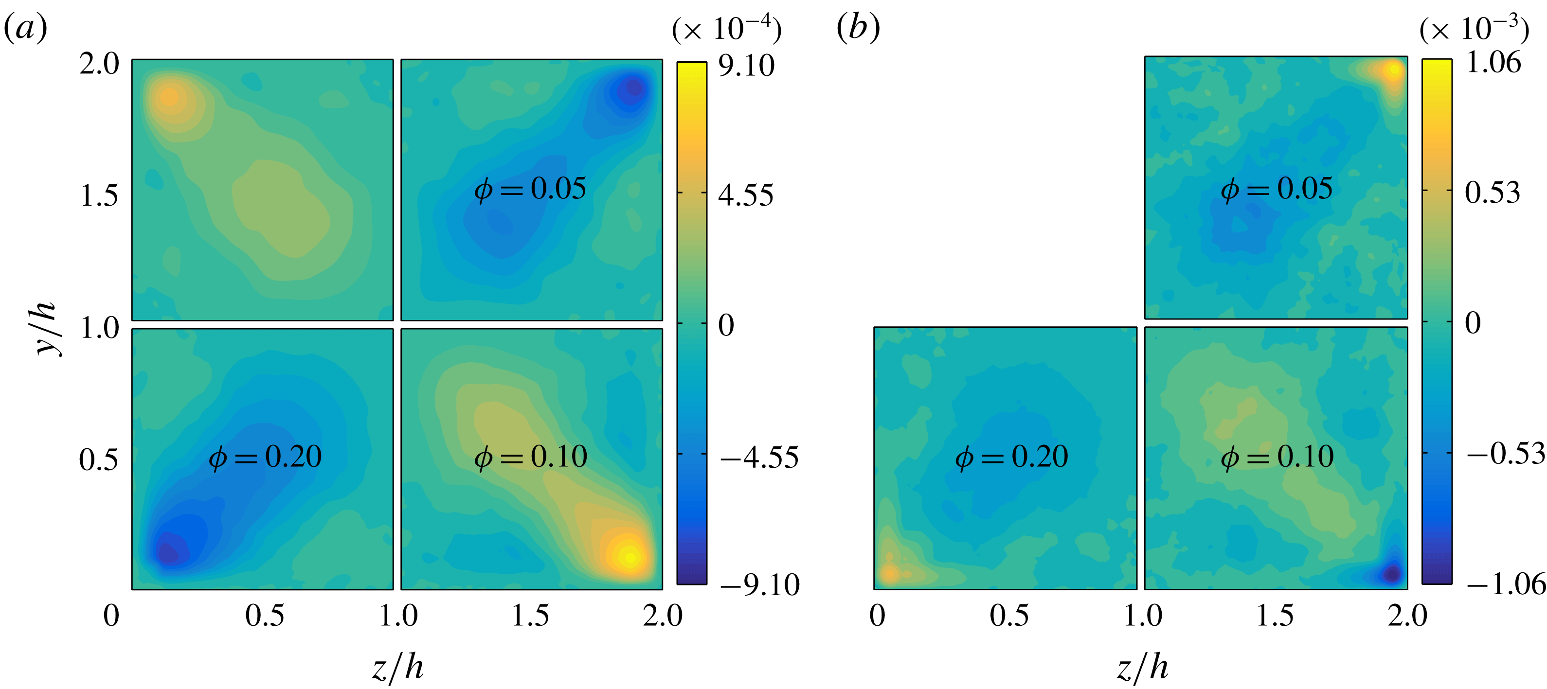
The contours of
 $\langle v_{f}^{\prime }w_{f}^{\prime }\rangle$
are shown in figure 16 for all
 $\unicode[STIX]{x1D719}$
. These are non-negligible along the corner bisectors (being directly related to mean secondary flows), and approximately one order of magnitude smaller than the primary Reynolds stress. Interestingly, we see that the maxima of
 $\langle v_{f}^{\prime }w_{f}^{\prime }\rangle$
strongly increases with
 $\unicode[STIX]{x1D719}$
up to
 $\unicode[STIX]{x1D719}=0.1$
and also for
 $\unicode[STIX]{x1D719}=0.2$
, the maximum value is still larger than that for
 $\unicode[STIX]{x1D719}=0.05$
. We also notice that regions of finite
 $\langle v_{f}^{\prime }w_{f}^{\prime }\rangle$
become progressively broader with increasing
 $\unicode[STIX]{x1D719}$
.
The secondary Reynolds stress of the solid phase,
 $\langle v_{p}^{\prime }w_{p}^{\prime }\rangle$
, resembles qualitatively that of the fluid phase, except at the corners were a high value of opposite sign is encountered. As a consequence, close to the corners this term may contribute in opposite way to the production or dissipation of vorticity with respect to
 $\langle v_{f}^{\prime }w_{f}^{\prime }\rangle$
.
We conclude this section by showing in figure 17 the mean streamwise fluid vorticity
 $\unicode[STIX]{x1D6FA}_{f}$
for all
 $\unicode[STIX]{x1D719}$
. The region of maximum vorticity at the wall is found between
 $z/h=0.2$
and
 $z/h=0.5$
for the unladen case and it extends closer to the corner for increasing
 $\unicode[STIX]{x1D719}$
. We also find that the maximum
 $\unicode[STIX]{x1D6FA}_{f}$
initially increases with the solid volume fraction (for
 $\unicode[STIX]{x1D719}=0.1$
the maximum
 $\unicode[STIX]{x1D6FA}_{f}$
is just slightly smaller than for
 $\unicode[STIX]{x1D719}=0.05$
). This is expected as also the intensity of the secondary motions increase. The contours of
 $\unicode[STIX]{x1D6FA}_{f}$
become more noisy for
 $\unicode[STIX]{x1D719}=0.2$
, with a maximum value below that of the single-phase case. Also, for
 $\unicode[STIX]{x1D719}=0.2$
the location of maximum
 $\unicode[STIX]{x1D6FA}_{f}$
is similar to that found for the unladen case.
Contours of the mean fluid streamwise vorticity
 $\unicode[STIX]{x1D6FA}_{f}$
(scaled by
 $h/U_{b}$
) for all
 $\unicode[STIX]{x1D719}$
under investigation.
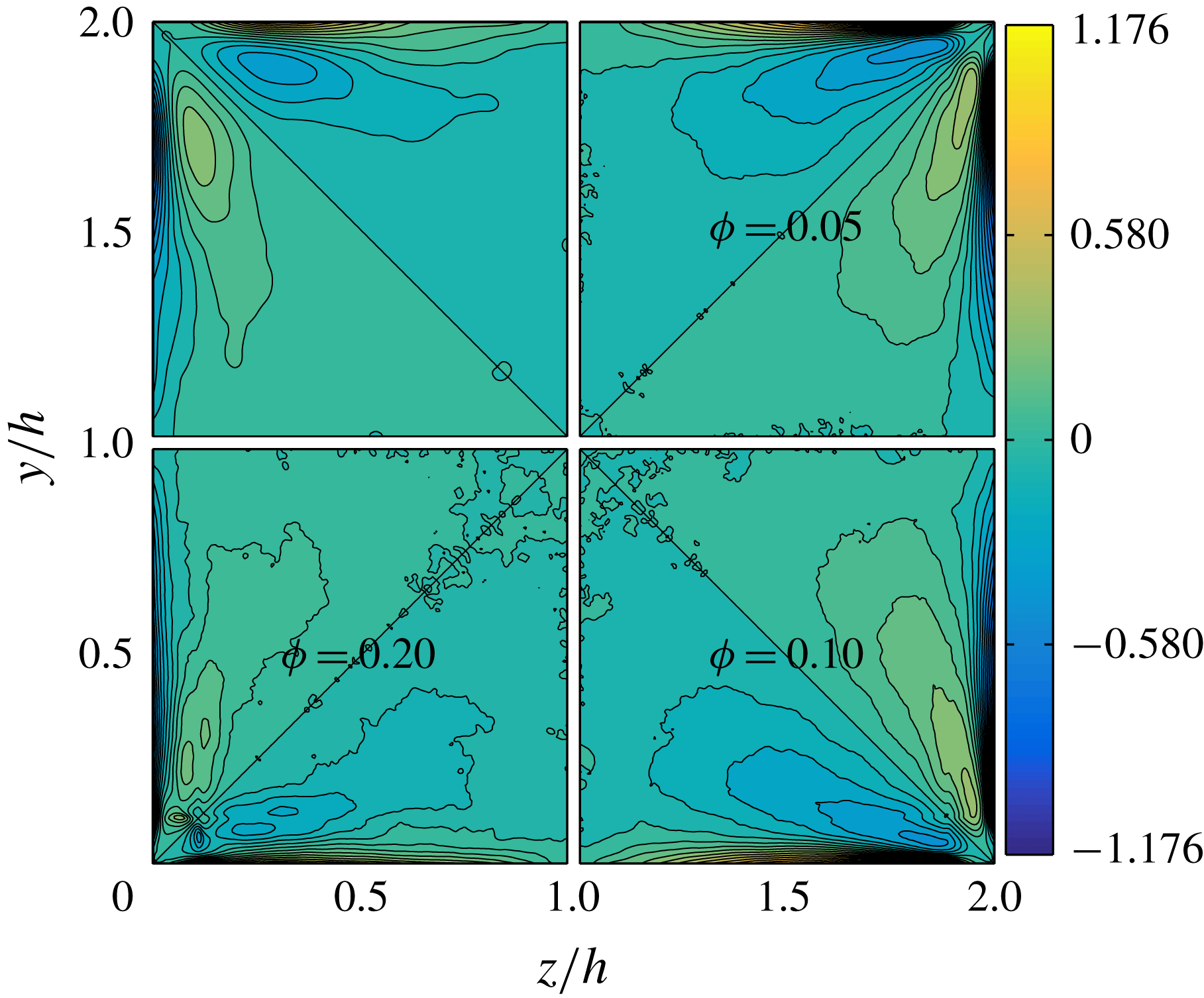
The mean streamwise vorticity attains a positive or negative sign in the near-wall region, depending on the specific octant considered. As we move further away from the walls, the mean streamwise vorticity changes sign. For the unladen case, the magnitude of the maximum vorticity at the walls is 2.5 times larger than the magnitude of the maximum vorticity of opposite sign found closer to the corner bisector. As reference and for clarity, we will consider the vorticity to be positive at the wall, and negative further away, as found for the top and bottom walls (for the lateral walls the situation is reversed). We find that the vorticity minimum approaches progressively the walls as
 $\unicode[STIX]{x1D719}$
increases up to
 $\unicode[STIX]{x1D719}=0.1$
, and that the ratio between the magnitudes of the maximum and minimum of vorticity increases up to
 ${\sim}3$
. On the other hand, for
 $\unicode[STIX]{x1D719}=0.2$
we clearly notice several local vorticity minima. One minimum is further away from the walls, at a location similar to what is found for the unladen case. Another minimum is further away towards the corner bisector. The other minimum is instead close to the corners. As we have previously shown, at the largest
 $\unicode[STIX]{x1D719}$
there is a significant mean particle concentration exactly at the corners and correspondingly we see two intense spots of vorticity around this location, antisymmetric with respect to the corner bisector.
Although (3.4) is valid for single-phase duct flow, we have calculated the convective, source/sink and diffusive terms for the cases of
 $\unicode[STIX]{x1D719}=0,0.05$
and 0.1. For
 $\unicode[STIX]{x1D719}=0.2$
there is a strong coupling between the dynamics of both fluid and solid phases, and it is therefore difficult to draw conclusions only by estimating the terms in (3.4).
As discussed by Gavrilakis (Reference Gavrilakis1992), the production of vorticity within the viscous sublayer is the main factor responsible for the presence of vorticity in the bulk of the flow. The main contribution to the production of vorticity is given by the term involving the gradients of the cross-stream normal stresses. For the unladen case, the maxima of this term are located close to the corners (at
 $y/h=0.016$
,
 $z/h=0.16$
from the bottom-left corner, similarly to what was found by Gavrilakis (Reference Gavrilakis1992)). Another positive, almost negligible contribution to the production of mean streamwise vorticity is given by the convective term. On the other hand, the diffusive term and the term involving the gradients of the secondary Reynolds stress give a negative contribution to the generation of vorticity in this inner-wall region. Note that the largest negative contribution due to the latter term is found close to the maximum production (
 $(y/h,z/h)=(0.016,0.15)$
for
 $\unicode[STIX]{x1D719}=0$
). Generally, we observe that the maximum production and dissipation increase and approach the corner as the volume fraction increases up to
 $\unicode[STIX]{x1D719}=0.1$
(not shown). In order to understand how the presence of particles contributes to the generation of vorticity, we calculate the ratio between the overall production and dissipation at the location of the maximum of the normal stress term (i.e. the summation of the convective term and the normal stress term, divided by the absolute value of the summation between the diffusive and secondary Reynolds stress terms). For the unladen case we have a good balance and the ratio is approximately 1. For
 $\unicode[STIX]{x1D719}=0.05$
and 0.1, the ratio is 0.96 and 0.95. Hence, the presence of the solid phase gives an additional contribution of approximately 5 % to the generation of mean streamwise vorticity in the near-wall region at the location of maximum production. The increased production due to larger gradients of the normal stress difference and due to the additional contribution by particles, leads globally to the larger
 $\unicode[STIX]{x1D6FA}_{f}$
observed at
 $\unicode[STIX]{x1D719}=0.05$
and 0.1.
3.5 Quadrant analysis
In this section we employ the quadrant analysis to identify the contribution from so-called ejection and sweep events to the production of
 $\langle u_{f}^{\prime }v_{f}^{\prime }\rangle$
and
 $\langle u_{f}^{\prime }w_{f}^{\prime }\rangle$
. In single-phase wall-bounded turbulent flows, it is known that these phenomena are associated with pairs of counter-rotating streamwise vortices that exist in the shear layer near the wall. These force low-momentum fluid at the wall towards the high-speed core of the flow. This is typically referred to as a Q2 or ejection event, with negative
 $u_{f}^{\prime }$
and positive
 $v_{f}^{\prime }$
. On the other hand, events with positive
 $u_{f}^{\prime }$
and negative
 $v_{f}^{\prime }$
are associated with the inrush of high-momentum fluid towards the walls and are known as sweeps or Q4 events. Events Q1 (positive
 $u_{f}^{\prime }$
and positive
 $v_{f}^{\prime }$
) and Q3 (negative
 $u_{f}^{\prime }$
and negative
 $v_{f}^{\prime }$
) are not associated with any particular turbulent structure when there is only one inhomogeneous direction. However, as discussed by Huser & Biringen (Reference Huser and Biringen1993) in turbulent duct flows these also contribute to the total turbulence production.
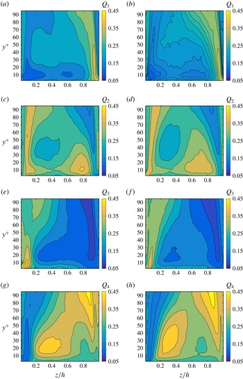
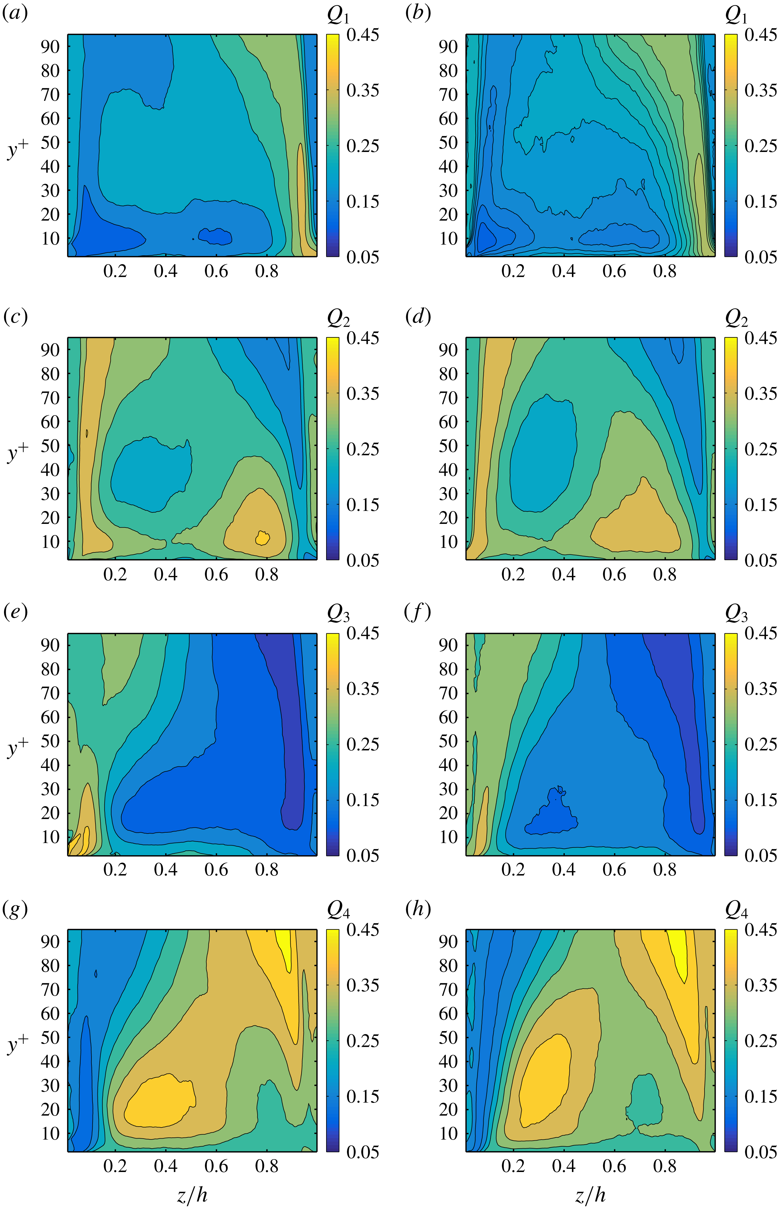
Maps of probability of Q1, Q2, Q3, Q4 events in panels (a), (c), (e), (g) and (b), (d), (f), (h) for particle volume fractions
 $\unicode[STIX]{x1D719}=0.0$
and 0.05, respectively.
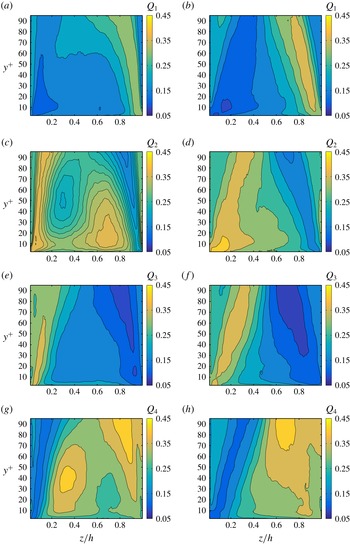
Maps of probability of Q1, Q2, Q3, Q4 events in panels (a), (c), (e), (g) and (b), (d), (f), (h) for particle volume fractions
 $\unicode[STIX]{x1D719}=0.1$
and 0.2, respectively.
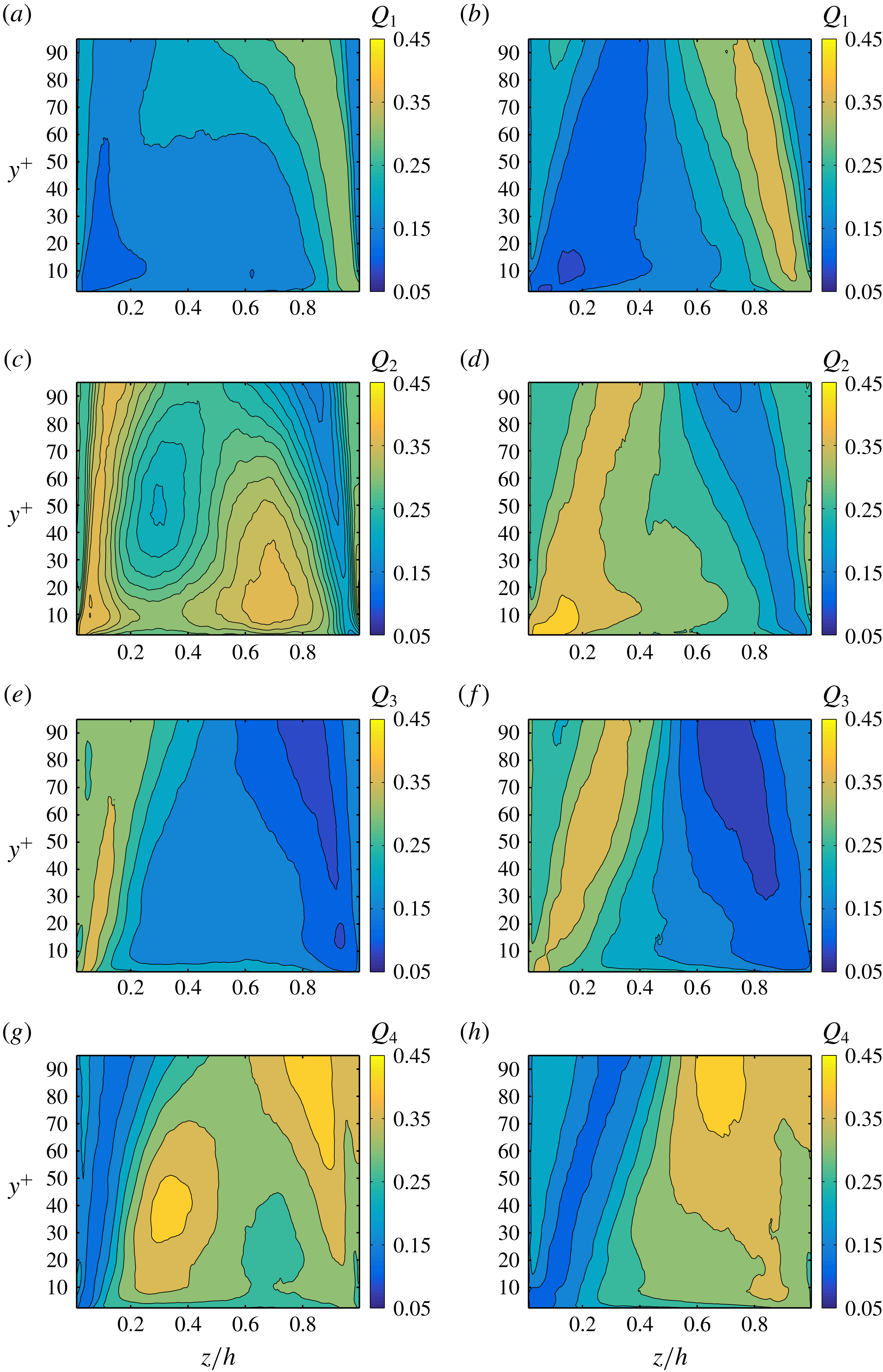
We first show contours of the probability of finding Q1, Q2, Q3, Q4 events for
 $\unicode[STIX]{x1D719}=0.0$
and 0.05 in figure 18, and for
 $\unicode[STIX]{x1D719}=0.1$
and 0.2 in figure 19. The maximum probability of an event is 1, so that the sum
 $\text{Q1}+\text{Q2}+\text{Q3}+\text{Q4}=1$
at each point. Since these events are typically important close to the walls, the
 $y$
-coordinate is reported in inner units (the viscous length at the wall bisector is chosen), while the wall-parallel
 $z$
-coordinate spans half of the duct. The contours of the probability of the different events directly enables us to easily compare and discuss all cases.
Results for the unladen case are substantially in agreement with those by Huser & Biringen (Reference Huser and Biringen1993) and Joung et al. (Reference Joung, Choi and Choi2007). Ejection (Q2) events are important at the wall bisector (
 $y/h=1$
) and around
 $y/h\sim 0.8$
. Joung et al. (Reference Joung, Choi and Choi2007) report strong Q2 events already
 $y/h=0.62$
, and this is probably due to the fact that their
 $Re_{b}$
was smaller than ours (
 $Re_{b}=4410$
instead of 5600). Q4 events are instead dominant closer to the vertical walls, around
 $y/h=0.3$
(as also reported by Joung et al. (Reference Joung, Choi and Choi2007)). Q3 events are found when both
 $u_{f}^{\prime }$
and
 $v_{f}^{\prime }$
are negative. As also shown by Huser & Biringen (Reference Huser and Biringen1993), we see that these increase from the wall bisector towards the vertical walls, being dominant at the corners. Consequently, these events are created by ejections from the vertical wall (and particularly from the corners), resulting in the increase of
 $\langle u_{f}^{\prime }v_{f}^{\prime }\rangle$
in this region.
The general picture is similar for
 $\unicode[STIX]{x1D719}=0.05$
and 0.1. The probability maps of Q1, Q2, Q3 and Q4 events are only slightly changed with respect to those of the unladen case. Concerning the probability of Q3 events we see that it is still higher at the corner and that it increases with
 $\unicode[STIX]{x1D719}$
along the vertical wall and along the corner bisector. It is clear from figure 19 that the turbulence activity is strongly reduced for
 $\unicode[STIX]{x1D719}=0.2$
. The probability of ejection and sweep events close to the walls is drastically reduced. The probability of sweep (Q4) events is around 35 % only in a small region close to the wall bisector (
 $y/h\sim 0.85$
). Instead, the probabilities of Q2 (ejections) and Q3 events are above 35 % in a region around the corner bisector, where we recall there is high mean particle concentration (
 $y/h\in (0;0.4)$
). At this volume fraction the probability of these events is therefore mostly correlated to fluid–particle interactions. The probability contours for
 $\unicode[STIX]{x1D719}=0.2$
are indeed very different from those at lower
 $\unicode[STIX]{x1D719}$
and from those of the unladen case. The absence of high probability regions of Q2 and Q4 events around
 $z/h\sim 0.8$
and
 $z/h\sim 0.3$
denotes the disruption of the coherent streamwise vortical structures.
The presence of two inhomogeneous directions allows us to extend the quadrant analysis to the secondary shear stress
 $\langle v_{f}^{\prime }w_{f}^{\prime }\rangle$
, which contributes to the production, dissipation and transport of mean streamwise vorticity, as discussed above. As in Huser & Biringen (Reference Huser and Biringen1993), to distinguish between the events related to the primary and secondary Reynolds stresses, we will refer to the latter as
 $\text{Q}1_{s},\text{Q}2_{s},\text{Q}3_{s}$
and
 $\text{Q}4_{s}$
events. These authors showed that as the corners are approached, contributions of the
 $\text{Q}1_{s}$
and
 $\text{Q}3_{s}$
events progressively decrease. On the other hand,
 $\text{Q}2_{s}$
and
 $\text{Q}4_{s}$
events are found to be stronger than the latter close to the corners. This is due to the interaction between ejections from both walls that tilt the ejection stem toward the perpendicular wall. We looked at probability maps of these events as previously done for the events related to the primary Reynolds stress. For the unladen case we see indeed that close to the corners the probability of having
 $\text{Q}2_{s}$
and
 $\text{Q}4_{s}$
events is substantially larger than that of
 $\text{Q}1_{s},\text{Q}3_{s}$
events (not shown). As we increase the volume fraction
 $\unicode[STIX]{x1D719}$
the probability of these events remains high until the highest
 $\unicode[STIX]{x1D719}=0.2$
is reached. In this case, we find that there is an approximately equal share of probability between all type of events indicating again that there is a substantial alteration of the turbulence and less structured flow in the presence of many particles.
4 Turbulent kinetic energy budget
In this section we investigate in more detail how the turbulence is altered by the presence of the solid particles. With this aim, we performed a turbulent kinetic energy budget. In the present simulations, the solid-phase contribution to the transport equation of turbulent kinetic energy is given by the mean value of the scalar product between the fluctuations of the immersed boundary force (
 $f_{IBM}^{\prime }$
) and the fluid velocity (
 $\boldsymbol{u}_{f}^{\prime }$
). As in Tanaka (Reference Tanaka2017), we name this as the interphase interaction term,
 ${\mathcal{I}}$
. At a statistically steady state, the transport equation of the turbulent kinetic energy,
 $k_{T}=0.5(u_{f,rms}^{\prime 2}+v_{f,rms}^{\prime 2}+w_{f,rms}^{\prime 2})$
, reads:
 $$\begin{eqnarray}\displaystyle U_{j}\frac{\unicode[STIX]{x2202}k_{T}}{\unicode[STIX]{x2202}x_{j}}=-\frac{\unicode[STIX]{x2202}T_{j}}{\unicode[STIX]{x2202}x_{j}}+P-\unicode[STIX]{x1D716}+\langle f_{IBM,j}^{\prime }u_{f,j}^{\prime }\rangle , & & \displaystyle\end{eqnarray}$$
where
 $P=-\langle u_{f,i}^{\prime }u_{f,j}^{\prime }\rangle (\unicode[STIX]{x2202}U_{f,i}/\unicode[STIX]{x2202}x_{j})$
is the production of the turbulent kinetic energy,
 $k_{T}$
,
 $\unicode[STIX]{x1D716}=\unicode[STIX]{x1D708}\langle (\unicode[STIX]{x2202}u_{f,i}^{\prime }/\unicode[STIX]{x2202}x_{j})(\unicode[STIX]{x2202}u_{f,i}^{\prime }/\unicode[STIX]{x2202}x_{j})\rangle$
is the dissipation of
 $k_{T}$
, while
 $T_{j}=0.5\langle u_{f,i}^{\prime }u_{f,i}^{\prime }u_{f,j}^{\prime }\rangle +\langle p^{\prime }u_{f,j}^{\prime }/\unicode[STIX]{x1D70C}_{f}\rangle -\unicode[STIX]{x1D708}(\unicode[STIX]{x2202}k_{T}/\unicode[STIX]{x2202}x_{j})$
represents the transport (i.e. diffusion) of
 $k_{T}$
. The term on the left-hand side represents instead the convection of turbulent kinetic energy. The terms appearing in (4.1) are calculated for all
 $\unicode[STIX]{x1D719}$
and normalized by
 $\langle U_{\ast ,0}\rangle ^{4}/\unicode[STIX]{x1D708}$
, where
 $\langle U_{\ast ,0}\rangle$
is the mean value of the friction velocity for the unladen case. We choose this value of the mean friction velocity in order to easily compare the cases at different
 $\unicode[STIX]{x1D719}$
, to understand whether the turbulence activity is reduced or not.
The values of the four terms on the right-hand side of (4.1) along the wall bisector are shown in figure 20(a–d) for all
 $\unicode[STIX]{x1D719}$
. The convective term is always
 ${\sim}0$
and it is hence not shown. We observe that the peak of the production,
 $P$
, initially increases with the volume fraction, from 0.25 for
 $\unicode[STIX]{x1D719}=0.0$
to approximately 0.28 for
 $\unicode[STIX]{x1D719}=0.1$
. For the unladen case, the production peak is at
 $y/h=0.063$
,
 $y^{+}=12$
. Instead, for
 $\unicode[STIX]{x1D719}=0.05$
and 0.1 it is located slightly closer to the wall (but still in the buffer layer), at
 $y/h=0.049$
,
 $y^{+}\simeq 9$
. Further increasing the volume fraction to
 $\unicode[STIX]{x1D719}=0.2$
, the production peak is replaced by two lower peaks at
 $y/h\simeq 0.04$
and
 $y/h\simeq 0.12$
. Their values are approximately 0.15 and 0.16, hence substantially smaller than the maximum of
 $P$
for the unladen case. This is related to the dense near-wall particle layer that disrupts coherent structures and reduces both ejection and sweep events, therefore reducing the production of turbulent kinetic energy. For
 $y/h>0.16$
(
 $y^{+}\simeq 30$
), the production is larger for all laden cases than for the unladen case. However, at equal
 $y/h$
the values for
 $\unicode[STIX]{x1D719}=0.2$
are smaller than those for
 $\unicode[STIX]{x1D719}=0.1$
. Therefore, the turbulence activity is increased with the volume fraction up to
 $\unicode[STIX]{x1D719}=0.1$
. For
 $\unicode[STIX]{x1D719}=0.2$
, due to large excluded volume effects it is instead reduced, at least with respect to the case at
 $\unicode[STIX]{x1D719}=0.1$
.
The four terms appearing in the transport equation of turbulent kinetic energy are shown along the wall bisector for
 $\unicode[STIX]{x1D719}=0.0$
(a),
 $\unicode[STIX]{x1D719}=0.05$
(b),
 $\unicode[STIX]{x1D719}=0.1$
(c) and
 $\unicode[STIX]{x1D719}=0.2$
(d):
 $P$
is the production,
 $\unicode[STIX]{x1D716}$
is the dissipation,
 $-\unicode[STIX]{x2202}T_{j}/\unicode[STIX]{x2202}x_{j}$
is the transport term and
 $I$
is the contribution due to the solid phase.
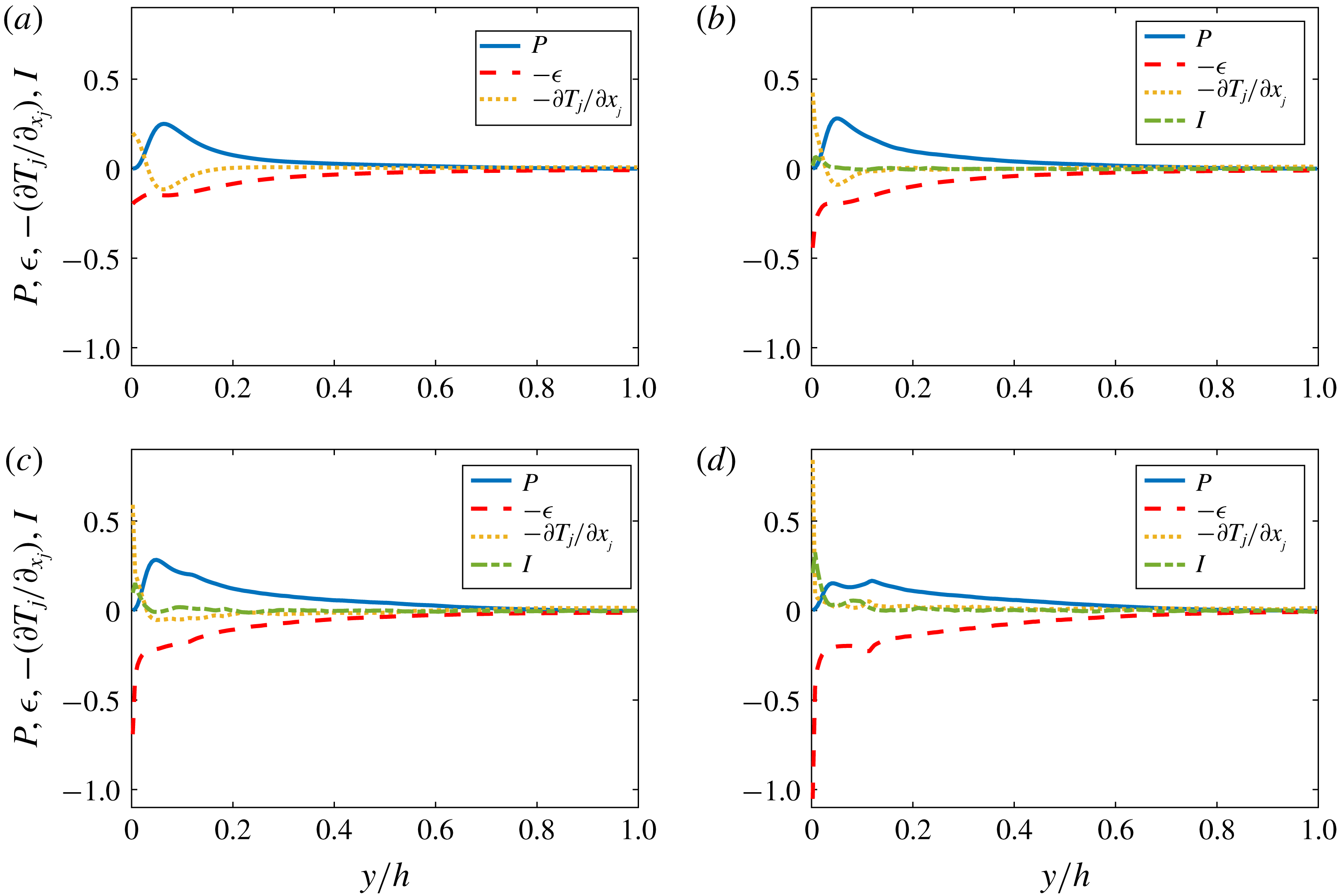
It is interesting to note that for the unladen case, the peak of production in the buffer layer is essentially balanced by the dissipation and transport terms. The transport terms that mostly balance the production are the turbulent and viscous diffusion terms,
 $0.5\langle u_{f,i}^{\prime }u_{f,i}^{\prime }u_{f,j}^{\prime }\rangle$
and
 $\unicode[STIX]{x1D708}(\unicode[STIX]{x2202}k_{T}/\unicode[STIX]{x2202}x_{j})$
(see also Vinuesa et al.
Reference Vinuesa, Noorani, Lozano-Durán, Khoury, Schlatter, Fischer and Nagib2014). However, as
 $\unicode[STIX]{x1D719}$
is increased, the production peak is progressively only balanced by the dissipation. The minimum of
 $-\unicode[STIX]{x2202}T_{j}/\unicode[STIX]{x2202}x_{j}$
progressively disappears, while its value at the wall increases. In particular, the pressure diffusion (
 $\langle p^{\prime }u_{f,i}^{\prime }/\unicode[STIX]{x1D70C}_{f}\rangle$
) and (especially) the viscous diffusion highly increase at the wall. Notice that the maximum of
 $-\unicode[STIX]{x2202}T_{j}/\unicode[STIX]{x2202}x_{j}$
increases from 0.2 for
 $\unicode[STIX]{x1D719}=0.0$
to 0.84 for
 $\unicode[STIX]{x1D719}=0.2$
. Hence, due to the high concentration of particles at the walls, there is also a larger redistribution of energy (i.e. the diffusion/transport of turbulent kinetic energy is enhanced).
Concerning the dissipation, it generally increases with
 $\unicode[STIX]{x1D719}$
. In particular, it drastically increases at the wall from 0.2 to 1.1 as
 $\unicode[STIX]{x1D719}$
increases from
 $\unicode[STIX]{x1D719}=0$
to 0.2. For
 $\unicode[STIX]{x1D719}=0.2$
, we also observe a second local maximum of
 $\unicode[STIX]{x1D716}$
at approximately
 $y/h=0.11$
, suggesting that the near-wall particle layer may act as a porous medium for the fluid phase. The larger dissipation at the wall is balanced by a progressive increase of the transport (
 $-\unicode[STIX]{x2202}T_{j}/\unicode[STIX]{x2202}x_{j}$
) and interphase interaction (
 ${\mathcal{I}}$
) terms. While for
 $\unicode[STIX]{x1D719}=0.05$
the contribution of the forth term in (4.1) is almost negligible, for larger
 $\unicode[STIX]{x1D719}$
this term increases substantially close to the wall. For
 $\unicode[STIX]{x1D719}=0.2$
this term is even larger than the production term. For all
 $\unicode[STIX]{x1D719}$
, the interphase interaction term contributes positively to the turbulent kinetic energy budget, i.e. effectively inject energy into the turbulent fluctuations. Notice that the maximum of
 ${\mathcal{I}}$
is located deep inside the viscous sublayer at
 $y^{+}\simeq 1.5$
(
 $y/h=0.007$
). The maximum of
 ${\mathcal{I}}$
is
 $\simeq 0.07,0.15$
and 0.32 for
 $\unicode[STIX]{x1D719}=0.05,0.1$
and 0.2.
The average over the cross-section of
 $P$
,
 $\unicode[STIX]{x1D716}$
,
 $-\unicode[STIX]{x2202}T_{j}/\unicode[STIX]{x2202}x_{j}$
and
 $I$
, for all
 $\unicode[STIX]{x1D719}$
.

Next, we report in figure 21 the values of
 $P,\unicode[STIX]{x1D716},-(\unicode[STIX]{x2202}T_{j}/\unicode[STIX]{x2202}x_{j})$
and
 ${\mathcal{I}}$
averaged over the cross-section. The mean production increases from 0.058 for the unladen case, to 0.079 for
 $\unicode[STIX]{x1D719}=0.1$
. Instead, for
 $\unicode[STIX]{x1D719}=0.2$
the mean value decreases below that for
 $\unicode[STIX]{x1D719}=0.05$
(0.065 and 0.074). Hence, the overall turbulence production is importantly reduced in the densest case (also explaining the observed turbulence attenuation). On the other hand, the mean dissipation increases monotonically with
 $\unicode[STIX]{x1D719}$
. Indeed, energy is mostly dissipated by friction with the duct walls and by the shear generated at the particles surfaces. The larger the number of particles (
 $\unicode[STIX]{x1D719}$
), the larger the energy dissipation. Finally, we find that both the mean transport and interphase interaction terms increase monotonically with
 $\unicode[STIX]{x1D719}$
. Hence, the presence of the solid phase leads to a stronger energy redistribution, and to an additional source of energy.
The particle Reynolds number,
 $Re_{p}=(2a)U_{s}/\unicode[STIX]{x1D708}$
, in one quadrant of the cross-section for all
 $\unicode[STIX]{x1D719}$
. Where
 $Re_{p}<0$
, the particles move faster than the fluid; whereas for
 $Re_{p}>0$
, the particles lag behind the fluid.
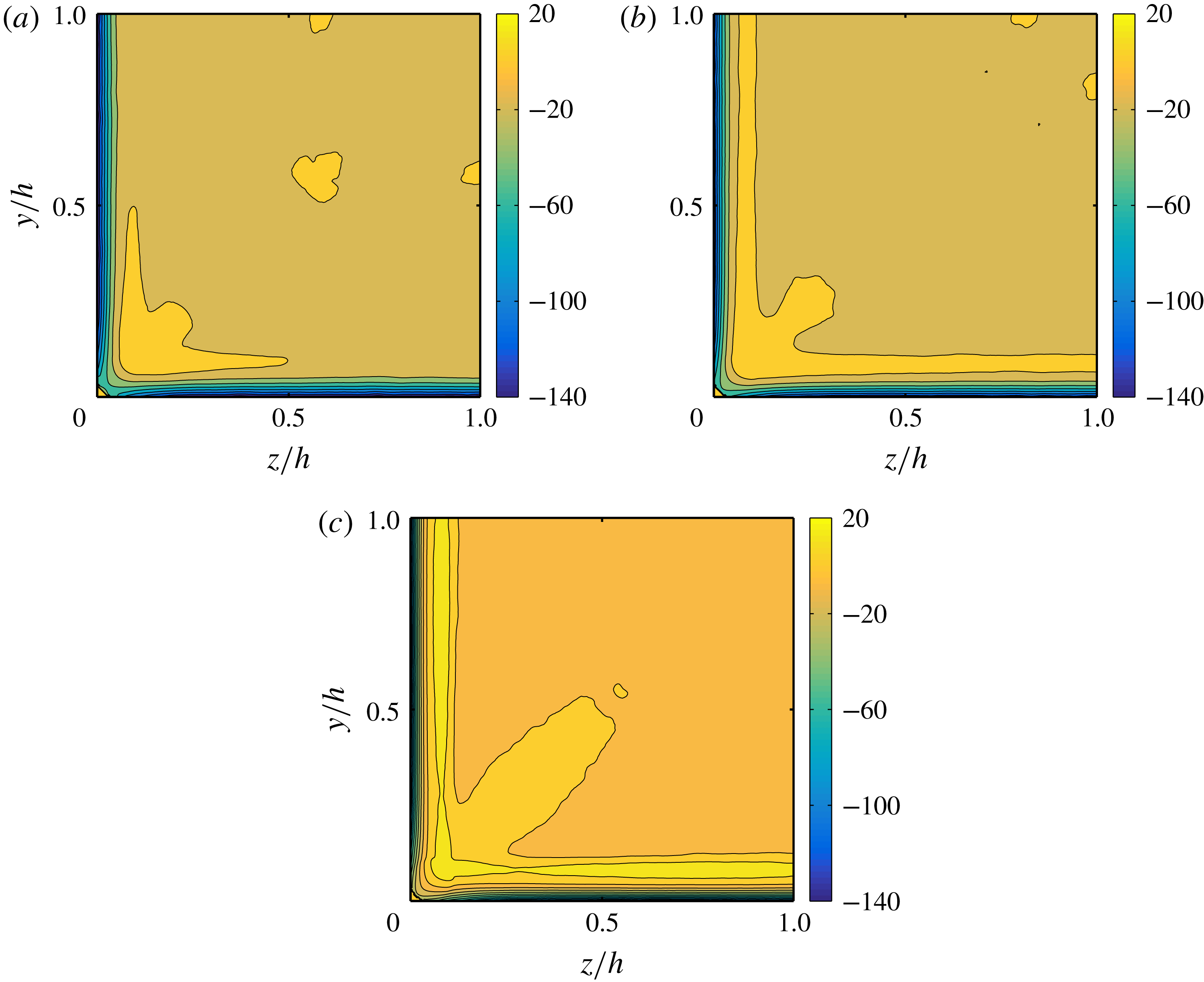
5 Particle dynamics
In this last section, we explore in more detail the dynamics of the solid phase. First of all, we calculate the difference between the mean streamwise fluid and particle velocities,
 $U_{s}(y,z)=U_{f}(y,z)-U_{p}(y,z)$
. This mean slip velocity is hence used to determine the particle Reynolds number,
 $Re_{p}=(2a)U_{s}/\unicode[STIX]{x1D708}$
, depicted in figure 22(a–c) for all
 $\unicode[STIX]{x1D719}$
. Notice that instead of defining it with
 $|U_{s}|$
, we use the actual value of the slip velocity; hence where
 $Re_{p}>0$
the particles lag behind the fluid and where
 $Re_{p}<0$
, the particles are faster than the fluid. We observe that
 $U_{p}(y,z)$
is larger than
 $U_{f}(y,z)$
, except near the corners and, for
 $\unicode[STIX]{x1D719}\geqslant 0.1$
, also slightly away from the walls. In regions where
 $U_{s}<0$
, the particle Reynolds number is of order
 $1$
towards the core of the duct, while it attains very large values (up to 140) near the walls. Indeed, at the walls the fluid velocity is zero due to the no-slip condition, while the velocity of the points on the particle surfaces is finite. On average, however, the particles move faster than the fluid with mean Reynolds numbers
 $|\langle Re_{p}\rangle |$
of 8.6, 7.0 and 3.6 (average performed over space and time).
We then focus on the regions where the particles lag behind the fluid (i.e.
 $U_{s}>0$
). For the cases at large
 $\unicode[STIX]{x1D719}\geqslant 0.1$
, the higher values of
 $U_{s}$
along the walls are located approximately at the same distances from the walls at which the particle layers are located (local maxima of particle concentration). In these particle layers close to the walls, particle–wall interactions are important. As a consequence particles are slowed down along their trajectories and the slip velocity is positive. Indeed, the mean streamwise hydrodynamic force on the particle in the near-wall region acts in the opposite
 $x$
-direction (not shown).
The regions of
 $U_{s}>0$
close to the corners deserve special attention, particularly for
 $\unicode[STIX]{x1D719}=0.05,0.1$
. First of all, we notice that the maximum positive
 $U_{s}$
is located on the bisector, very close to the corner (between
 $y/h=z/h=0.07$
and 0.1). Here the particle Reynolds number,
 $Re_{p}$
, is between 14 and 20, for all cases. Moving along the diagonals towards the duct core,
 $U_{s}$
progressively decreases becoming zero almost precisely at the locations of maximum particle concentration (
 $y/h=z/h=0.23,0.29$
for
 $\unicode[STIX]{x1D719}=0.05,0.1$
), see figure 6(a,b). Therefore, there appears to be a correlation between the slip velocity and the local particle concentration. Indeed, as shown by Saffman (Reference Saffman1965) (Liu et al.
Reference Liu, Xue, Sun and Hu2016, see also), a sphere in a Poiseuille flow that lags behind the fluid experiences a lift force towards the channel centre. In analogy, particles that lag behind the fluid experience a force that pushes them away from the corners. Further away along the corner bisectors, the slip velocity is mostly negative and the force towards the centre is small, and
 $Re_{p}$
almost never exceeds values larger than 5.
To further understand the dynamics, we investigate the hydrodynamic forces acting on the particles. The distribution in one quadrant of the cross-section of the mean vertical hydrodynamic force,
 $F_{y}/(\unicode[STIX]{x1D70C}_{f}U_{b}^{2}a^{4}/(2h)^{2})$
is shown in figure 23(a–c) for all
 $\unicode[STIX]{x1D719}$
. For the data in the figure, we have saved the hydrodynamic forces acting on each particle centroid and averaged over the streamwise direction and time on a new spatial grid. Notice that the chosen mesh is 1.5 times coarser than that of the simulation (
 $\unicode[STIX]{x0394}x^{\prime }=\unicode[STIX]{x0394}3x/2$
), a choice necessary to avoid excessively noisy distributions, while still faithfully representing the dynamics. In addition, the first point shown is slightly larger than
 $a/h$
(0.057 instead of 0.056). This will be important later on for the discussion of the collision forces in the wall-normal direction.
Distribution of the mean vertical hydrodynamic force acting on the particles for
 $\unicode[STIX]{x1D719}=0.05$
(a), 0.1 (b) and 0.2 (c) displayed over one quadrant of the cross-section. In (d) we show the mean hydrodynamic force
 $F_{y}$
along the corner bisector.
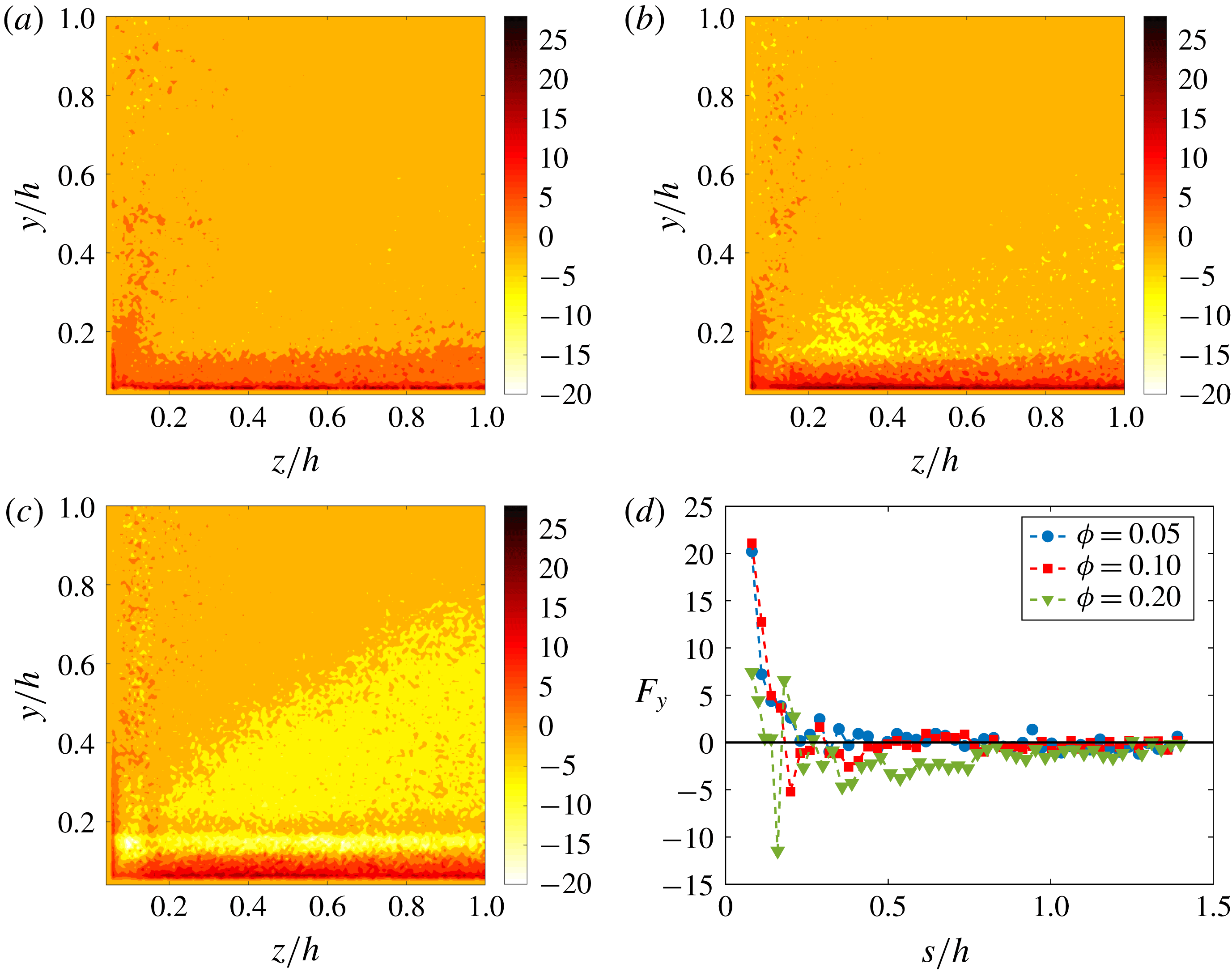
From figure 23(a–c) we clearly see that the wall-normal hydrodynamic force is strong close to the walls and directed away from them. Hence, the particles experience a lift force that pulls them away from the walls. For
 $\unicode[STIX]{x1D719}=0.2$
there is a very clear formation of a near-wall layer of particles. From figure 23(c) we see that the hydrodynamic force that is first directed away from the wall, for
 $y/h>0.13$
changes sign, reaching quickly a minimum negative value (i.e. the force is towards the wall). The location of the minimum negative force is at
 $y/h\sim 0.16$
. For larger
 $y/h$
, the mean force first increases to
 ${\sim}0$
and then it decreases reaching another minimum at
 $y/h\sim 0.23$
. After this minimum, the force remains negative and decreases as the core is approached. Finally,
 $F_{y}$
becomes approximately zero for
 $y/h\geqslant 0.8$
(the force is actually slightly negative). Therefore, particles tend to reside longer in the core region due to the very small
 $F_{y}$
. For
 $y/h<0.8$
particles experience forces that tend to push them towards the walls, which is maximum in modulus at
 $y/h\sim 0.16$
. However, if/when they get too close to the walls they are repelled from it. The repulsive force from the walls can be the result of a slip shear-induced lift (Saffman Reference Saffman1965) and a short-range viscous force between particles and walls. The weaker force that pushes the particles towards the walls may be due to the curvature of the mean velocity profile, similarly to what happens in laminar flows (Ho & Leal Reference Ho and Leal1974; Liu et al.
Reference Liu, Xue, Sun and Hu2016). Notice that for
 $\unicode[STIX]{x1D719}\leqslant 0.1$
, the mean wall-normal hydrodynamic force decreases quickly to
 ${\sim}0$
for
 $y/h>0.2$
. Consequently, the particles are more uniformly distributed in the cross-section.
It is then particularly interesting to observe the behaviour of the hydrodynamic force along the corner bisector. With this aim, we depict in figure 23(d)
 $F_{y}/(\unicode[STIX]{x1D70C}_{f}U_{b}^{2}a^{4}/(2h)^{2})$
as a function of
 $s=\sqrt{(y/h)^{2}+(z/h)^{2}}$
, with
 $s=0$
at the origin (the corner), and
 $s=\sqrt{2}h$
at the core. For
 $\unicode[STIX]{x1D719}=0.05$
, the profiles of
 $F_{y}/(\unicode[STIX]{x1D70C}_{f}U_{b}^{2}a^{4}/(2h)^{2})$
seem to confirm our speculation on the role of the slip velocity,
 $U_{s}$
. We see indeed that the force is approximately zero for
 $s$
greater than the value corresponding to the maximum concentration (
 $s\simeq 0.33h$
). For smaller
 $s$
, the force is strongly repulsive. For
 $\unicode[STIX]{x1D719}=0.1$
, the picture is not as clear. The force crosses zero for
 $s\sim 0.18h$
and reaches a minimum for
 $s\sim 0.20h$
. The force then oscillates around zero and another clear minimum is found close to the location of maximum concentration,
 $s\sim 0.41h$
. Finally, the force becomes again approximately zero for
 $s\simeq 0.50h$
. The new location of high particle concentration is hence due to the combined effect of hydrodynamic and collision forces (with neighbour particles) as will be discussed later.
We have also examined the magnitude of the mean cross-stream hydrodynamic forces acting on the particles,
 $\left(\sqrt{F_{y}^{2}+F_{z}^{2}}\right)\!/(\unicode[STIX]{x1D70C}_{f}U_{b}^{2}a^{4}/(2h)^{2})$
(contours not shown). For
 $\unicode[STIX]{x1D719}\leqslant 0.1$
,
 $\sqrt{F_{y}^{2}+F_{z}^{2}}$
is generally smaller along the corner bisectors than in the rest of the cross-section (being approximately zero at
 $s\simeq 0.33h$
for
 $\unicode[STIX]{x1D719}=0.05$
), which may explain why particles reside longer on the corner bisectors. Instead, for
 $\unicode[STIX]{x1D719}=0.2$
,
 $\sqrt{F_{y}^{2}+F_{z}^{2}}$
is lowest in the core region (
 $y/h\geqslant 0.8$
). Here
 $\sqrt{F_{y}^{2}+F_{z}^{2}}\sim 0$
and, accordingly, the concentration is large.
Distribution of the mean vertical collision force acting on the particles for
 $\unicode[STIX]{x1D719}=0.05$
(a), 0.1 (b) and 0.2 (c) displayed over one quadrant of the cross-section. In (d) we show the combination of the mean hydrodynamic and collision forces,
 $F_{y}+F_{y}^{c}$
along the corner bisector.
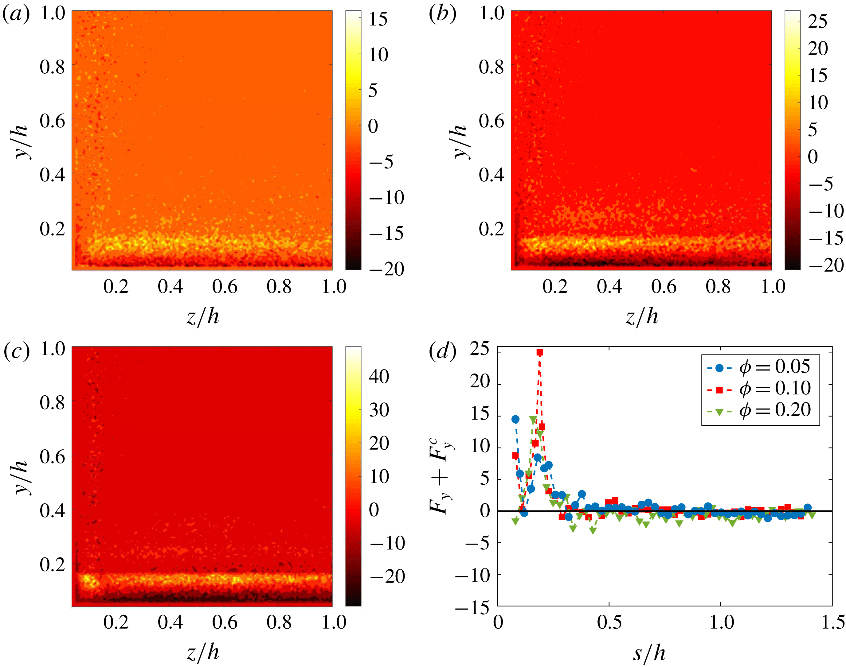
We conclude this last section by discussing the mean collision forces between particles. These are also extracted from the simulations, binned in the cross-section and shown in figure 24(a–c). As previously stated, the first point of the chosen mesh is at
 $0.06h$
from the wall. Consequently, the particle–wall collisions, occurring when the particle centroids are located at distances of
 $0.056h$
from the walls, are not captured. Results concerning the particle–wall collisions will be discussed later. The mean vertical collision force between particles,
 $F_{y}^{c}/(\unicode[STIX]{x1D70C}_{f}U_{b}^{2}a^{4}/(2h)^{2})$
, is typically opposed to the hydrodynamic force: at near-wall locations where particles are strongly repelled from the walls (
 $F_{y}>0$
), the collision force is directed towards the walls (
 $F_{y}^{c}<0$
). When particles move away from the walls, they tend to collide with particles that are ‘above’ them. The larger the volume fraction
 $\unicode[STIX]{x1D719}$
, the larger the number of particles surrounding the reference particle, and the larger the average collision force. On the contrary, for
 $y/h\geqslant 0.13$
, where the hydrodynamic force is (generally) directed towards the walls, collision forces are directed towards the core. Finally, in figure 24(d) we report the summation of the mean hydrodynamic and collision forces,
 $F_{y}+F_{y}^{c}$
, along the corner bisector (described by the coordinate
 $s$
). For
 $\unicode[STIX]{x1D719}=0.05,0.1$
, the overall force acting on the particles is still repulsive close to the walls. However, the initial high value of the hydrodynamic force is reduced by the opposing collision force. Due to the negative collision force, the overall force then attains a minimum around
 $s\sim 0.12$
. Further increasing
 $s$
, the collision force changes sign and the overall repulsive force reaches a maximum. The overall force then decreases becoming approximately zero for
 $s\geqslant 0.33h$
, for all
 $\unicode[STIX]{x1D719}$
. Note that this is the location of maximum particle concentration for
 $\unicode[STIX]{x1D719}=0.05$
. Concerning the case at
 $\unicode[STIX]{x1D719}=0.2$
, the hydrodynamic cross-stream forces directed away from the core are actually slightly larger than zero (in magnitude), even close to the core (as can be seen from figure 23
d). However, at this large
 $\unicode[STIX]{x1D719}$
, when a particle is pushed away from the core, it encounters many neighbour particles that hinder its motion. The collision force on the particle is hence opposed to the hydrodynamic force, and we find that the combination of these forces is approximately zero in the core region (
 $s\geqslant 0.9h$
), as shown in figure 24(d). Hence, the large particle concentration at the core is the result of small wall-normal hydrodynamic forces and counteracting collision forces.
To conclude, we examine the particle–wall collisions; these substantially increase with the volume fraction
 $\unicode[STIX]{x1D719}$
. To estimate these, we have considered only cases for which particles are almost precisely at contact with a wall (at distance of
 $(a+0.001)/h$
). We hence estimated a mean collision force
 $\langle F^{c,w}\rangle /(\unicode[STIX]{x1D70C}_{f}U_{b}^{2}a^{4}/(2h)^{2})$
that is seen to increase from 11.6 for
 $\unicode[STIX]{x1D719}=0.05$
, to
 $19.3$
for
 $\unicode[STIX]{x1D719}=0.1$
. Finally, for
 $\unicode[STIX]{x1D719}=0.2$
 $\langle F^{c,w}\rangle$
further increases to 23.8. It is interesting to notice that the mean collision force does not increase linearly with the volume fraction,
 $\unicode[STIX]{x1D719}$
. Instead, we see a saturation at large
 $\unicode[STIX]{x1D719}$
, which may be due to the fact that at
 $\unicode[STIX]{x1D719}=0.2$
, many of the particles migrate towards the core of the duct, therefore colliding less with particles that are close to the walls. Further, we have previously shown an important turbulence attenuation at the same volume fraction. The turbulent r.m.s. velocities are reduced and consequently, turbulent structures push the particles towards the walls with lower momentum, leading to a reduction of the overall collision force with the walls.
6 Final remarks
We have studied turbulent duct flows laden with suspensions of finite-size particles, particles larger than the smallest flow structures. We have considered neutrally buoyant rigid spheres of size
 $a=h/18\sim 10\unicode[STIX]{x1D6FF}_{\ast }$
and three solid volume fractions
 $\unicode[STIX]{x1D719}=0.05,0.1,0.2$
. The bulk Reynolds number has been set to
 $Re_{b}=5600$
to compare results with those found for turbulent channel flow of similar
 $h/a$
and
 $Re_{b}$
. For the unladen duct, this choice of
 $Re_{b}$
results in a mean friction Reynolds number
 $Re_{\unicode[STIX]{x1D70F}}=185$
and friction factor of
 $0.035$
(same value that is obtained via the empirical formula of Jones Reference Jones1976).
One of the main findings concerns the effect of the particle presence on the so-called secondary/cross-flow velocities of the fluid phase. In single-phase turbulent duct flows their magnitude is approximately 2 % of the bulk velocity. We have found that the intensity of these secondary flows progressively increases with solid volume fraction up to
 $\unicode[STIX]{x1D719}=0.1$
. Above this volume fraction, a strong turbulence activity attenuation is found and correspondingly the maximum value of the cross-flow velocity magnitude sharply drops below the value of the unladen case. Interestingly, we have found a lag between fluid and particle cross-flow velocities. In particular, at the corner bisectors the fluid cross-flow velocity is larger than that of the solid phase. On the contrary, the fluid and particle cross-flow velocities are similar at the walls away from the corners. It is well known that at the wall bisectors these secondary flows convect low-momentum fluid from the walls towards the duct core. This induces a convexity in the mean fluid streamwise velocity isotach (i.e. at equal distance from the walls, the mean streamwise velocity is larger at the corner bisector than at the wall bisector). As the cross-flow velocity increases with
 $\unicode[STIX]{x1D719}$
, so does the convexity of the mean streamwise velocity contours. For
 $\unicode[STIX]{x1D719}=0.2$
the convexity is less than in the unladen case. For all
 $\unicode[STIX]{x1D719}$
, the mean streamwise velocity of the solid phase is similar to that of the fluid, except very close to the walls were the particle velocity is not subjected to the no-slip condition.
At the wall bisector, the mean streamwise velocity profiles are found to be similar to those in channel flows. In particular, as
 $\unicode[STIX]{x1D719}$
increases, the velocity decreases closer to the walls and increases towards the core. For
 $\unicode[STIX]{x1D719}=0.2$
we have found a more abrupt increase in velocity than what was previously found in channel flows. We have also reported the mean streamwise velocity in inner units and calculated the von Kármán constant,
 $\unicode[STIX]{x1D705}$
, and the additive coefficient
 $B$
. For the unladen case we have obtained the same
 $\unicode[STIX]{x1D705}$
found by Gavrilakis (Reference Gavrilakis1992) for
 $Re_{b}=4410$
. On increasing
 $\unicode[STIX]{x1D719}$
both
 $\unicode[STIX]{x1D705}$
and
 $B$
are found to decrease, denoting a contrasting behaviour in terms of drag reduction or enhancement. The friction Reynolds number calculated at the wall bisector,
 $Re_{\unicode[STIX]{x1D70F},bis}$
is found to increase for all
 $\unicode[STIX]{x1D719}$
, as in channel flow, although the increase is smaller than in the latter flow case at equal
 $\unicode[STIX]{x1D719}$
. Concerning the mean friction Reynolds number, we find that it increases up to
 $\unicode[STIX]{x1D719}=0.1$
in a similar fashion to what is observed in channel flow. Instead, for
 $\unicode[STIX]{x1D719}=0.2$
the mean friction Reynolds number is similar to that for
 $\unicode[STIX]{x1D719}=0.1$
(it is actually 0.5 % larger). We believe that this is due to a stronger turbulence attenuation than is found in channel flow. Indeed, the near-wall particle concentration is approximately doubled with respect to what is found in channel flow. Quasi-coherent streamwise structures are rapidly disrupted by particles and the frequency of ejection and sweep events is reduced. Following this line of thought, we also performed a turbulent kinetic energy budget. We indeed find that the turbulence production increases up to
 $\unicode[STIX]{x1D719}=0.1$
. However, for
 $\unicode[STIX]{x1D719}=0.2$
the mean production is less than for
 $\unicode[STIX]{x1D719}=0.05$
. So there is indeed an important turbulence attenuation. In contrast, the dissipation and the transport of turbulent kinetic energy increase monotonically with
 $\unicode[STIX]{x1D719}$
. Therefore, due to the interaction with solid particles a larger fraction of the turbulent kinetic energy is dissipated. Since the mean turbulence production is reduced, the enhanced dissipation is balanced by a stronger diffusion of energy and by the additional interphase interaction term, due to the presence of solid particles. This extra term contributes positively to the turbulent kinetic energy budget, and increases monotonically with
 $\unicode[STIX]{x1D719}$
in a similar way as the transport term.
Other important observations concern the mean particle concentration. Particles tend to form a stable layer very close to the walls for all
 $\unicode[STIX]{x1D719}$
. However, for
 $\unicode[STIX]{x1D719}\leqslant 0.1$
, the higher particle concentration is on the corner bisectors close to the corner (at a distance of approximately
 $0.27h$
). The high particle concentration at the corners is probably related to the existence of the secondary flows. Eventually, it results from the observed lag between the fluid and solid phases cross-flow velocities. It should be noted that in laminar duct flows of similar
 $h/a$
and
 $Re_{b}\sim 500$
particles are also found to mostly accumulate at the corners (Kazerooni et al.
Reference Kazerooni, Fornari, Hussong and Brandt2017). In the latter case this is a result of the particle inertial migration away from the duct core. For
 $\unicode[STIX]{x1D719}=0.2$
, the particle concentration close to the corners is still high, but the maximum concentration is found at the duct core. This observation is in contrast to what is found in channel flow, revealing the importance of confinement on particle dynamics. From the data available for channel flow, we have indeed found that there is a substantial number of particles crossing the periodic boundaries (i.e. a significant particle diffusion in the spanwise direction). The additional confinement due to the vertical walls induces therefore a different particle concentration.
Examining the fluid and particles velocity fluctuations, we see that close to the walls there is a redistribution of energy towards a more isotropic state (i.e. decrease of the streamwise r.m.s. velocity with
 $\unicode[STIX]{x1D719}$
and an increase of the fluctuation velocities in the cross-stream directions). For
 $\unicode[STIX]{x1D719}=0.2$
all components of the r.m.s. velocity are found to be smaller than those of the unladen case, except for the spanwise and wall-normal components close to the corners. Looking at the primary Reynolds stress, we have seen that it increases throughout the cross-section up to
 $\unicode[STIX]{x1D719}=0.1$
. It is interesting to note that for turbulent channel flow, Picano et al. (Reference Picano, Breugem and Brandt2015) found that the maximum
 $\langle u_{f}^{\prime }v_{f}^{\prime }\rangle ^{+}$
decreases with
 $\unicode[STIX]{x1D719}$
. On the other hand, we have here found that at the wall bisector the maximum is approximately constant up to
 $\unicode[STIX]{x1D719}=0.1$
. So the turbulence activity reduction becomes important for volume fractions larger than
 $\unicode[STIX]{x1D719}=0.1$
as can be seen from the results obtained for
 $\unicode[STIX]{x1D719}=0.2$
.
Interestingly, close to the corners the secondary Reynolds stress
 $\langle v_{f}^{\prime }w_{f}^{\prime }\rangle$
, is larger than in the single-phase case for all
 $\unicode[STIX]{x1D719}$
. The secondary Reynolds stress of the solid phase,
 $\langle v_{p}^{\prime }w_{p}^{\prime }\rangle$
, resemble those of the fluid, except at the corners where they change sign. Therefore they may represent an additional source of mean streamwise vorticity. Indeed, close to the corners and in the viscous sublayer, the gradients of the fluid secondary Reynolds stress typically act as a sink of mean streamwise vorticity (the production of vorticity within the viscous sublayer is mainly responsible for the presence of vorticity in the bulk of the flow). The opposite sign may indicate that this new contribution due to the solid phase actually acts as a source term.
We have then performed quadrant analyses of both primary and secondary Reynolds stresses, looking at the occurrence probability of Q1, Q2, Q3 and Q4 events in the cross-section. The probabilities are everywhere similar up to
 $\unicode[STIX]{x1D719}=0.1$
, again indicating that the turbulence is not strongly altered up to this solid volume fraction. However, for
 $\unicode[STIX]{x1D719}=0.2$
the probability maps change drastically denoting a strong reduction of the turbulence activity.
Finally, we have studied more in detail the particle dynamics for each volume fraction. First of all, we have computed the slip velocity between fluid and particles. On average, the particles are found to move faster than the fluid, except in the near-wall region and at the corners where they are slower. For
 $\unicode[STIX]{x1D719}=0.05$
and 0.1 the location of maximum particle concentration along the corner bisectors is precisely where the slip velocity vanishes. Closer to the corners, the particles lag the fluid and this could be responsible for a lift force directed towards the core (Saffman Reference Saffman1965; Liu et al.
Reference Liu, Xue, Sun and Hu2016). By estimating the mean wall-normal forces on the particles (the summation of the hydrodynamic and collision forces), we see indeed that particles are pushed away from the corners. The mean wall-normal hydrodynamic force generally acts to repel the particles from the walls. Between the near-wall region and the core, this force is generally small and directed towards the walls, especially for
 $\unicode[STIX]{x1D719}=0.2$
. Finally, in the core region it becomes approximately zero. For
 $\unicode[STIX]{x1D719}=0.2$
we find that the mean wall-normal hydrodynamic force is actually (slightly) smaller than zero along the corner bisectors. Hence, although hydrodynamic forces are small around the core, particles would leave more often this region (mostly along the bisectors). However, at this large
 $\unicode[STIX]{x1D719}$
, particles are surrounded by many neighbours, and experience collision forces that hinder their motion. Consequently, the resulting mean force on the particles is approximately zero, and the large concentration at the core is observed.
Acknowledgements
This work was supported by the European Research Council grant no. ERC-2013-CoG-616186, TRITOS. Computer time was provided by SNIC (Swedish National Infrastructure for Computing). The authors also acknowledge the support from the COST Action MP1305: Flowing matter.