1 Introduction
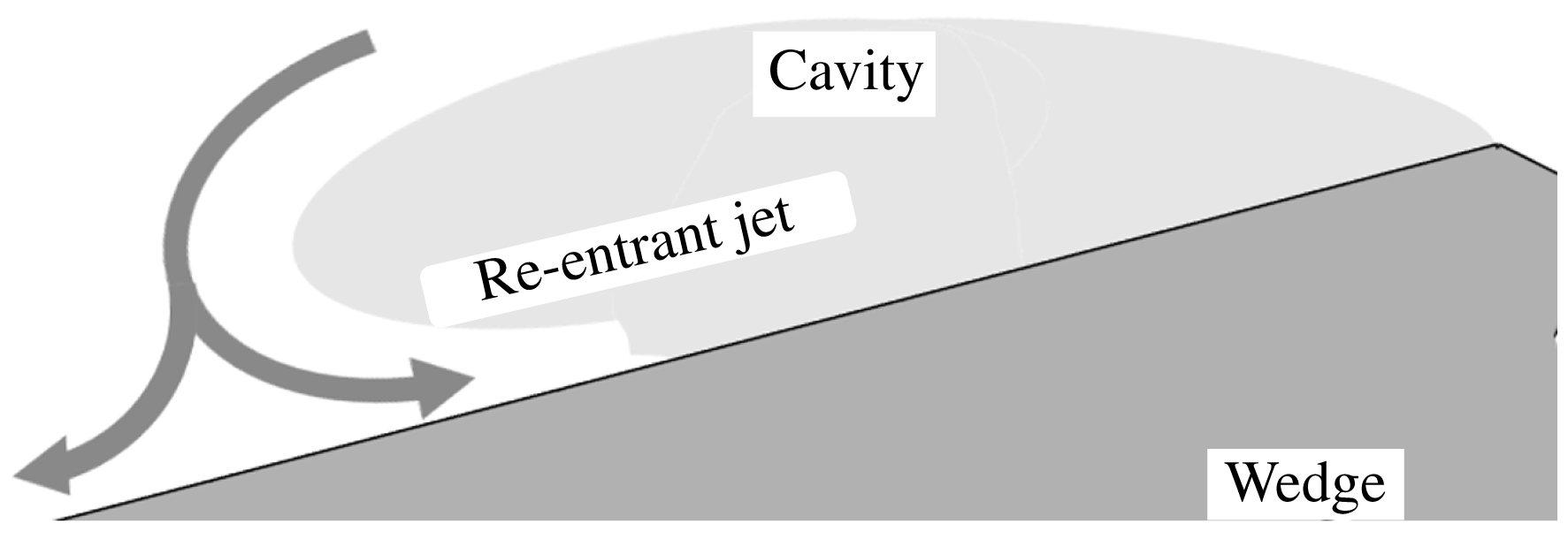
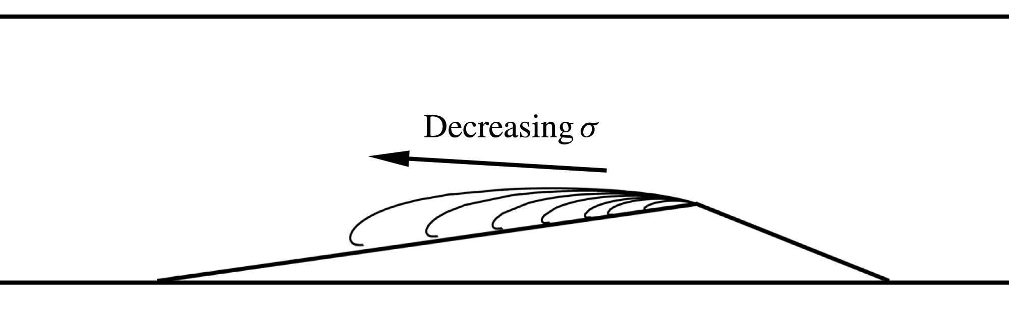
Hydrodynamic cavitation is a phenomenon characterized by phase change from liquid to vapour at nearly constant temperatures in low-pressure regions of a flow field. Partial cavitation occurs when the low-pressure regions produced by separated shear flows are filled with vapour, forming a cavity. Flows exhibiting partial cavitation include separated shear layers on the suction side of lifting surfaces, the blades of turbo machines, inducers of cryogenic rocket motors and passages of high-pressure diesel fuel injectors. Once formed, partial cavities are often stable, but under certain conditions can experience auto-oscillations of lengths that are characterized by the shedding of vapour clouds, termed as cloud cavitation. The cavity volume oscillations can be intermittent or periodic, and have adverse effects such as loss of lift, vibration and erosion. The occurrence of cloud cavitation is often related to the presence of re-entrant flow in the closure region of the cavity which forms as the liquid flow outside the cavity reattaches in the closure region. A schematic representation of a re-entrant liquid flow is shown in figure 1. Many studies have verified the existence, development and the role of liquid re-entrant flow on cavitation dynamics and cloud shedding.
Classical re-entrant flow in the cavity closure that leads to vapour cloud pinch off. The flow is from right to left.

Furness & Hutton (Reference Furness and Hutton1975), using a potential-flow-based numerical method, computed the structure of the re-entrant flow on a convergent–divergent nozzle until it intersected the cavity interface. They found the results to be in reasonable comparison with experiments. Lush & Skipp (Reference Lush and Skipp1986) also attributed the occurrence of periodic shedding to re-entrant jets. Visualization of re-entrant jets on cavitating flows has also been reported by Le, Franc & Michel (Reference Le, Franc and Michel1993) using dye injection on a plano-convex hydrofoil and by de Lange (Reference de Lange1996) using a transparent two-dimensional hydrofoil model. The presence of the re-entrant jet, and its role in cloud shedding on a two-dimensional hydrofoil, was verified in a study by Kawanami et al. (Reference Kawanami, Kato, Yamaguchi, Tanimura and Tagaya1997). By placing an obstacle in the path of the re-entrant jet generated on a hydrofoil, they found that auto-oscillations vanished, suggesting the re-entrant jet has a prominent role. Partial cavitation studies on objects with spanwise geometric variations, such as hydrofoils with sweep, have also been studied by Crimi (Reference Crimi1970), Bark (Reference Bark1985), Bark (Reference Bark1986), Ihara, Watanabe & Shizukuishi (Reference Ihara, Watanabe and Shizukuishi1989) and de Lange (Reference de Lange1996). Unlike a two-dimensional cavity with a cavity closure line perpendicular to the flow direction, the closure line for three-dimensional cavities can be oriented in a direction that is geometry dependent. This would result in the re-entrant jet having a different orientation and dynamics. Laberteaux & Ceccio (Reference Laberteaux and Ceccio2001b ) found that a three-dimensional geometry can sustain stable cavities with re-entrant flow. They found that re-entrant flow was directed away from the cavity, making it stable. However, this does not mean that three-dimensional geometries cannot experience periodic shedding. Foeth, van Terwisga & van Doorne (Reference Foeth, van Terwisga and van Doorne2008) made an informative study of partial cavitation dynamics on a twisted foil. They found that periodic shedding was indeed observed, and a re-entrant jet with a component along the spanwise direction caused the pinching off vapour clouds.
The conditions necessary for the development of a re-entrant jet, and subsequent periodic shedding, has been explored in detail for canonical two-dimensional geometries. Callenaere et al. (Reference Callenaere, Franc, Michel and Riondet2001), in a seminal study, explored cavitation dynamics in a two-dimensional geometry. They mapped different regimes of flow with no shedding, periodic re-entrant jet observation with no shedding and re-entrant jet-induced periodic shedding. They found the importance of the role of the adverse pressure on the development of the re-entrant flow that resulted in periodic shedding. Gopalan & Katz (Reference Gopalan and Katz2000) in their study on cavitation in a nozzle found that a re-entrant jet developed when the cavity closure was in the region of adverse pressure. Laberteaux & Ceccio (Reference Laberteaux and Ceccio2001a ) also found that partial cavitation on wedges where the cavity was not in a region with a strong adverse pressure gradient and did not experience re-entrant flow, and hence no shedding, but rather experienced a turbulent frothy wake. They suggested the importance of the flow in the closure of the cavity and its role in dictating the phase transfer and the development of the re-entrant jet. Le et al. (Reference Le, Franc and Michel1993) measured the pressure distribution in a partial cavity on a plano-convex foil, at different attack angle and cavitation number combinations, for constant cavity lengths. They found that the pressure distribution for cavities with re-entrant flow and shedding was different from non-shedding open cavities, with the maximum pressure having much lower values.
These studies on different geometries suggest that the existence of a re-entrant flow is not sufficient for periodic shedding of clouds. Diagnosis of the cavitating flow field has also been done to understand the relationship of the measurements to the observed dynamics. Kubota et al. (Reference Kubota, Kato, Yamaguchi and Maeda1989) performed comprehensive unsteady measurements of the velocity field of a cavitating flow over a hydrofoil using conditionally sampled laser Doppler velocimetry. They found the convection velocity of the cloud to be much lower than the free-stream speed. Kawanami et al. (Reference Kawanami, Kato, Yamaguchi, Maeda and Nakasumi2002) used laser holography to study the structure of a cloud shed from a hydrofoil and estimated the bubble size distribution. Measurements of the re-entrant flow underneath the cavity using electrical impedance probes was done by Pham, Larrarte & Fruman (Reference Pham, Larrarte and Fruman1999) and George, Iyer & Ceccio (Reference George, Iyer and Ceccio2000). Callenaere et al. (Reference Callenaere, Franc, Michel and Riondet2001) measured the thickness of the re-entrant jet using acoustic probes and found shedding to be dependent on the jet thickness, with thicker re-entrant jets resulting in shedding. Foeth et al. (Reference Foeth, van Doorne, van Terwisga and Wieneke2006) used time-resolved particle image velocimetry and flow visualization techniques to estimate the interfacial velocity of a cavitation on a twisted hydrofoil. They found that the velocity at the interface of the cavity was very close to that estimated using a simple streamline model.
Measurements inside a partial cavity can greatly enhance the understanding of cavitation dynamics and have been done previously. Void fraction distribution measurements within a Venturi flow were performed by Stutz & Reboud (Reference Stutz and Reboud1997a ) and Stutz & Reboud (Reference Stutz and Reboud1997b ). Using optical probes, they measured the conditionally averaged void fraction and the liquid-phase flow velocity of cloud shedding. They also observed the presence of reversed liquid flow, and reported a maximum measured void fraction of 0.21. They also performed detailed flow measurements using laser Doppler velocimetry (LDV) to characterize the outer liquid flow, and optical probes to measure the void-fraction distribution and liquid-phase velocity in an attached sheet cavity. They found the presence of a re-entrant flow that results in a stable cavity and used simple mass balance relations to estimate the vapour flow coefficient. They reported a maximum void fraction of nearly 80 % in the cavity near the line of detachment. Stutz & Legoupil (Reference Stutz and Legoupil2003) used X-ray densitometry to non-intrusively measure the void fraction in a geometry similar to Stutz & Reboud (Reference Stutz and Reboud1997a ). The set-up consisted of a single row of 24 detectors that could acquire void-fraction profiles along a line at a rate of 1000 samples per second. The measurements were compared with optical probes, and it was found that the maximum void fraction for the case of periodic shedding was approximately 25 %. Coutier-Delgosha et al. (Reference Coutier-Delgosha, Stutz, Vabre and Legoupil2007) used the same diagnostic set-up to measure void-fraction profiles on a plano-convex foil. They reported maximum averaged void-fraction values of close to 60 %, with instantaneous values exceeding 85 %. Mäkiharju et al. (Reference Mäkiharju, Gabillet, Paik, Chang, Perlin and Ceccio2013) recently developed an X-ray densitometry system that measures the time-resolved two-dimensional projection of the void-fraction flow field of gas–liquid flows, and this system was utilized for the present study. Time-resolved measurements of void-fraction flow fields can provide information about various vapour generation and destruction processes that play a key role in the onset of periodic cloud shedding.
Simple potential flow-based analytical methods can predict broad flow features such as cavity shapes, lengths and thicknesses of re-entrant flow of partial cavities forming on separated flows. There are many analytical tools (Milne-Thomson Reference Milne-Thomson1968; Wu Reference Wu1972; Brennen Reference Brennen2013) available for the prediction of cavity shape in a given geometry, taking into account the presence of a re-entrant liquid flow that is in kinematic equilibrium with the mean flow. Since one of the goals of the present study is to understand the dynamics of vapour production and re-entrant flow generation, comparison of the experimental observations with the predictions of a cavitation model using simple free-streamline methods can provide more insights into the formation of the re-entrant flow. Such a comparison will provide information about the importance of flow processes in different regimes, the limits on the flow turning angle of a liquid re-entrant flow and the closeness of the actual observations with those predicted by these simple models.
During the course of our investigation we discovered that re-entrant flow is not solely, or even, primarily responsible for sheet-to-cloud transition for the partial cavities under study. The cavities under investigation formed at the apex of a wedge that has a sharp line of flow separation. Based on the void-fraction measurements it was found that averaged void fraction in the cavity ranged from less than 5 % at higher cavitation numbers to values exceeding 50 % under shedding conditions. It is well known that the sound speed of high-void-fraction cavitation bubbly mixtures is greatly reduced compared to that of the constituent water, air and vapour (Shamsborhan et al. Reference Shamsborhan, Coutier-Delgosha, Caignaert and Nour2010). This makes such mixtures compressible and susceptible to shocking under certain flow conditions. Such mixtures can experience abrupt changes in the local void fraction due to the propagation of condensation shocks (Crespo Reference Crespo1969; Noordzij & Van Wijngaarden Reference Noordzij and Van Wijngaarden1974; Brennen Reference Brennen2005), and bubbly shock propagation has been related to the collapse of shed cavitation clouds (Reisman, Wang & Brennen Reference Reisman, Wang and Brennen1998). In the present study, we have observed bubbly shocks within the separated region of the partial cavity and related the shock propagation to the shedding cycle of cavitation clouds in a mechanism which is distinct from the classically described re-entrant jet.
We begin by describing the experimental set-up in § 2. In § 3 we detail the free-streamline formulation of the analytical solution of two-dimensional cavitating flow over a wedge. The general trends of experimentally observed cavitation dynamics and the variation of cavity length with inlet cavitation number are presented and compared with free-streamline results in § 4 along with the observed cavitation dynamics for the wedge at different speeds and cavitation numbers. In § 5 we show how the propagating discontinuity in void fraction observed within the cavity is a condensation shock, and in § 6 we show how the transition from intermittent to strongly periodic shedding can be related to the cavity Mach number. Our conclusions are presented in § 7.
2 Experimental set-up
Experiments were carried out at the University of Michigan 9-Inch Water Tunnel. The tunnel has a
 $6:1$
round contraction leading into a test section with a diameter of 23 cm (9 inches). The test section then transitions to a square cross-section that is 21 by 21 cm with chamfered corners. The flow velocity in the tunnel test section can be varied from
 $U_{0}=0$
to 18 m s
 $^{-1}$
and the static pressure,
 $p_{0}$
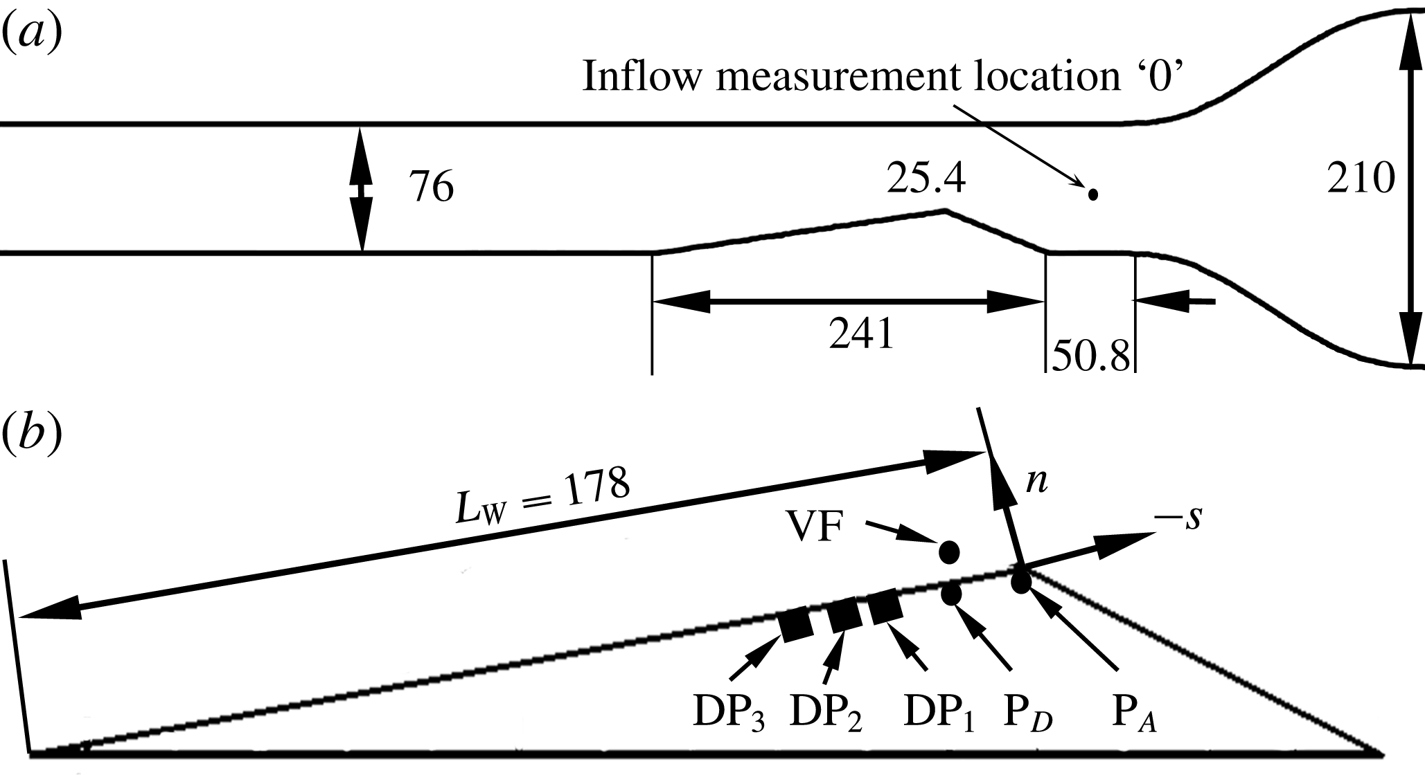
, from near vacuum to 200 kPa. A de-aeration system enables the control of the dissolved air content. In the present experiments, the test section was further reduced in area to a conduit that had a 7.6 cm by 7.6 cm cross-section. This was done to reduce the baseline X-ray attenuation produced by the non-cavitating flow.
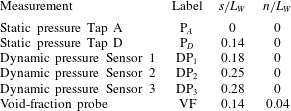
(a) Schematic diagram of the secondary contraction within the test section of the water channel, with dimensions in millimetres; the reduced test section is 76 mm square, and the side view illustrates the placement of the wedge. (b) The wedge model with locations of the static and dynamic pressure measurements; the location for the dynamic void-fraction measurement is also shown.

Measurement location for sensors shown in figure 2(b).

2.1 Wedge geometry and inflow properties
The wedge geometry was chosen because it produces a nominally two-dimensional cavity with a well-defined line of cavity detachment. The wedge makes an angle of
 $22.1^{\circ }$
to the incoming flow, and has a downstream angle of
 $8.1^{\circ }$
. The height of the wedge was chosen to produce a contraction ratio of
 $2/3$
at the wedge apex when placed in the reduced test section of the water channel. A schematic of the wedge in the water tunnel is shown in figure 2(a). The static pressure at the entrance to the secondary test section, designated as ‘0’, in figure 2(a), was measured using an Omega Engineering PX20-030A5V, 0 to 208 kPa, absolute pressure transducer with stated accuracy of 0.08 % of full scale. The pressure difference between the test section inlet and upstream of the primary contraction was measured using an Omega Engineering PX409030DWU10V, 0 to 208 kPa, differential pressure transducer with an accuracy of 0.08 % of full scale. Based on the measurement of the differential pressure, and the area ratios, the velocity at the entrance flow speed into the reduced test section was calculated. The velocity at the inlet of the secondary test section was fixed at
 $U_{0}=6$
, 8, and 10 m s
 $^{-1}$
, with an uncertainty of
 $\pm 0.1~\text{m}~\text{s}^{-1}$
. The pressure upstream of the wedge at the inlet was varied between
 $35<p_{0}<150$
kPa with an uncertainty of
 $\pm$
2 kPa. The inlet cavitation number,
 $\unicode[STIX]{x1D70E}_{0}$
, is defined as
 $$\begin{eqnarray}\displaystyle \unicode[STIX]{x1D70E}_{0}=\frac{(p_{0}-p_{V})}{{\textstyle \frac{1}{2}}\unicode[STIX]{x1D70C}U_{0}^{2}}, & & \displaystyle\end{eqnarray}$$
where
 $p_{V}$
is the vapour pressure of water and
 $\unicode[STIX]{x1D70C}$
is the water density. The inlet cavitation number,
 $\unicode[STIX]{x1D70E}_{0}$
, was varied from 4.5 to 1.6. The dissolved oxygen content was maintained at approximately 50 % at standard conditions.
2.2 Average and dynamic surface pressure measurements
Static pressure was measured at two locations, Tap A and Tap D, on the wedge surface. Tap A was located very close to the wedge apex and Tap D was located further downstream from the wedge apex in the cavity. The taps were 0.8 mm in diameter at the wedge surface and the average pressure was measured using an Omega Engineering PX20-05A5V 0 to 36 kPa transducer with an accuracy of 0.08 % of full scale. To prevent the lines from out gassing, the tubes were purged with de-aerated water from the tunnel and the transducer was placed at a height of 610 mm below the tap location in the direction of gravity. This additional head prevented the out gassing of vapour in the lines and the final pressures were corrected with this head value. The unsteady pressure on the wedge surface was also measured using flush mounted surface pressure probes. A PCB 138M101 transducer connected to a ICP Sensor 480CO2 signal conditioner was embedded in the wedge model to perform the unsteady pressure measurements. The unsteady pressure signals were sampled at a frequency of 250 kHz using a National Instruments PCI-MIO-16E-4 DAQ card triggered using the common time base with the X-ray measurement system.
2.3 High-speed video set-up
The cavitating flow around the wedge was synchronously imaged from the top and side using two Vision Research Phantom v730 high-speed video cameras for 8 m s
 $^{-1}$
and filmed only from the side view for 6 and 10 m s
 $^{-1}$
. The flow was illuminated using two Arrilux lamps and the cameras were triggered using a signal generator. The frame rate of the video recordings was 4000 f.p.s., with a 35 ms exposure time. For the side view, a Nikon 90 mm lens was used to record a viewing area of 265 by 115 mm with each pixel corresponding to 0.2 mm and for the top view, a Nikon 35–55 mm lens to record a viewing area of 300 by 200 mm with a pixel size of 0.25 mm at the middle of the wedge along streamwise direction. The recordings were post-processed in MATLAB to resize the images such that the pixels-per-mm scales matched. The cameras were synchronized using the Phantom Cine Control software and were triggered using a TTL signal generated by a Stanford DG-535 delay generator. More information about the experimental set-up can be found at Ganesh (Reference Ganesh2015).
2.4 Cinemagraphic X-ray densitometry system
A cinematographic X-ray densitometry system was used to measure the spatial distribution of the void fraction for the cavitating flow around a wedge. A complete description of the system is provided by Mäkiharju (Reference Mäkiharju2012) and Mäkiharju et al. (Reference Mäkiharju, Gabillet, Paik, Chang, Perlin and Ceccio2013); a brief description is provided here. The X-ray densitometry system had a source capable of 433 mA at 150 kV and the imaging system is comprised of an image intensifier coupled with a high-speed camera (Vision Research Phantom V9.0). X-ray densitometry-based void-fraction measurements are based on the principle that the fraction of photons of any one specific photon energy that is not attenuated is related to the mass attenuation coefficients, densities and thicknesses of all the materials present along the path of the beam. Based on the Beer–Lambert law, for a domain with
 $N$
distinct materials we can write
 $$\begin{eqnarray}\displaystyle \frac{I}{I_{0}}=\text{e}^{(\mathop{\sum }_{i=1}^{N}(x_{n}\unicode[STIX]{x1D70C}_{n}/\unicode[STIX]{x1D707}_{n}))}, & & \displaystyle\end{eqnarray}$$
where
 $I_{0}$
is the original intensity of the beam,
 $I$
is the intensity of the beam transmitted by passing through
 $n$
materials with corresponding mass attenuation coefficient of
 $\unicode[STIX]{x1D707}_{n}/\unicode[STIX]{x1D71A}_{n}$
, density
 $\unicode[STIX]{x1D71A}_{n}$
and the mass thickness is
 $x_{n}$
. The attenuation coefficient is a known property of photon energy of any material in the domain and is related to the material density and its atomic properties. Therefore, for a single material,
 $N=1$
, a measure of the change in intensity can be converted into a measure of the average density of the material along the beam path. In the case of two-phase gas–liquid flows, we can obtain a quantitative measure of the void fraction,
 $\unicode[STIX]{x1D6FC}$
, which is given by,
 $$\begin{eqnarray}\displaystyle \unicode[STIX]{x1D6FC}=\frac{\ln \left(\displaystyle \frac{I_{m}}{I_{w}}\right)}{\ln \left(\displaystyle \frac{I_{a}}{I_{w}}\right)}. & & \displaystyle\end{eqnarray}$$
This equation provides the void fraction along any given beam path through a test section as a function of the intensities,
 $I$
, of photon fluxes having passed through a test section filled with a mixture
 $m$
, all water
 $w$
or all air
 $a$
, at any one given photon energy. The accuracy of the void-fraction measurement has been validated against those obtained by use of water phantoms representative of the observed void fractions. An estimate for the maximum void fraction was attained by using water phantoms, and this calibration sets the maximum grey-scale value for the camera. The root mean square difference (RMSD) uncertainty of absolute void fraction for any pixel in a single (non-time-averaged) frame is approximately 5 %, and approximately 1 % for time-averaged data. The spatial resolution of the X-ray system is 0.25 mm for the averaged void-fraction flow field, and the recordings are made at the rate of 1000 f.p.s. A more comprehensive discussion on the technique, its uncertainty and the potential sources for error was provided by Mäkiharju et al. (Reference Mäkiharju, Gabillet, Paik, Chang, Perlin and Ceccio2013). The system works on the principle of Beer–Lambert’s law of attenuation of ionised radiation based on the composition of the attenuator. In this case, the attenuation from the X-ray measurements, average void fraction,
 $\langle \unicode[STIX]{x1D6FC}\rangle$
and RMSD void fraction,
 $\unicode[STIX]{x1D6FC}^{\prime }$
, can be calculated using the following relations:
 $$\begin{eqnarray}\displaystyle & \displaystyle \langle \unicode[STIX]{x1D6FC}(x,y)\rangle =\frac{\displaystyle \mathop{\sum }_{t=1}^{N}\unicode[STIX]{x1D6FC}(x,y,t)}{N}, & \displaystyle\end{eqnarray}$$
 $$\begin{eqnarray}\displaystyle & \displaystyle \unicode[STIX]{x1D6FC}^{\prime }(x,y)=\sqrt{\frac{\left(\langle \unicode[STIX]{x1D6FC}(x,y)\rangle -\displaystyle \mathop{\sum }_{t=1}^{N}\unicode[STIX]{x1D6FC}(x,y,t)\right)^{2}}{N}}. & \displaystyle\end{eqnarray}$$
 $N$
, was approximately 780. The images were recorded at a sample rate of 1000 f.p.s. and the spatial resolution of a pixel corresponded to 0.125 mm.
3 Free-streamline model of the two-dimensional wedge flow
Two-dimensional flow over the wedge sustaining a partial cavity with a constant cavity pressure can be modelled using free-streamline theory. Assuming an irrotational, incompressible and inviscid flow, the two components of velocities can be written as,
 $$\begin{eqnarray}\displaystyle & \displaystyle u=-\frac{\unicode[STIX]{x2202}\unicode[STIX]{x1D713}}{\unicode[STIX]{x2202}y}=\frac{\unicode[STIX]{x2202}\unicode[STIX]{x1D719}}{\unicode[STIX]{x2202}x}, & \displaystyle\end{eqnarray}$$
 $$\begin{eqnarray}\displaystyle & \displaystyle v=\frac{\unicode[STIX]{x2202}\unicode[STIX]{x1D713}}{\unicode[STIX]{x2202}x}=\frac{\unicode[STIX]{x2202}\unicode[STIX]{x1D719}}{\unicode[STIX]{x2202}y}. & \displaystyle\end{eqnarray}$$
Equations (3.1) and (3.2), by virtue of satisfying the Cauchy–Riemann relations, facilitate the use of complex analytic functions to represent flow fields. Since a cavity has constant pressure, and hence velocity, at the interface, solution of a partial cavity forming on a wedge amounts to finding a suitable complex function that satisfies given geometric and kinematic boundary conditions. In addition, for partial cavities, the pressure along the interface can be assumed to be a constant. Representing the velocity as the gradient of the velocity potential, we can define, on the boundary of the cavity
 $F(x,y)=0$
,
 $$\begin{eqnarray}\displaystyle \unicode[STIX]{x1D735}\unicode[STIX]{x1D719}\boldsymbol{\cdot }\unicode[STIX]{x1D735}F(x,y)=0. & & \displaystyle\end{eqnarray}$$
The dynamic boundary condition on the cavity interface is given by
 $$\begin{eqnarray}\displaystyle (\unicode[STIX]{x1D735}\unicode[STIX]{x1D719})^{2}=U^{2}(1+\unicode[STIX]{x1D70E}), & & \displaystyle\end{eqnarray}$$
where
 $\unicode[STIX]{x1D70E}$
is the cavitation number based on the constant cavity pressure,
 $p_{C}$
.
 $$\begin{eqnarray}\displaystyle \unicode[STIX]{x1D70E}=\frac{(p-p_{C})}{\frac{1}{2}\unicode[STIX]{x1D70C}U^{2}}=\frac{{q_{c}}^{2}}{U^{2}}-1. & & \displaystyle\end{eqnarray}$$
With the aforementioned background, the method can now be applied to the present study. The free-streamline model of the two-dimensional cavity flow adopted in the present study is based on that of Wu, Whitney & Brennen (Reference Wu, Whitney and Brennen1971). The present approach is very close to that of Laberteaux & Ceccio (Reference Laberteaux and Ceccio2001a
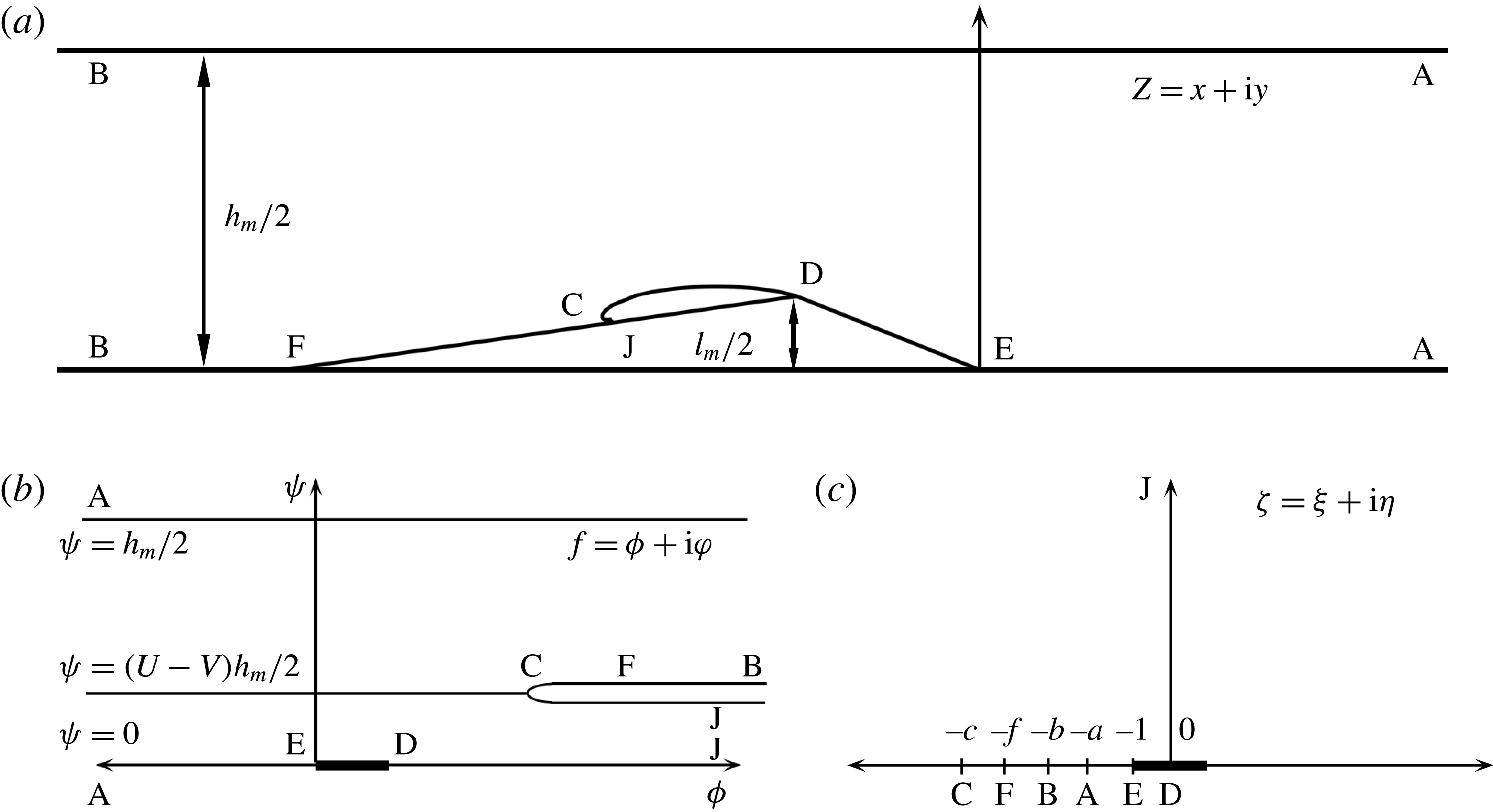
). Figure 3(a) represents the flow over the wedge in the physical plane
 $Z$
. The free-stream cavitation number features as a parameter that dictates the cavity shape, as suggested in (3.5). The free streamline separates at the apex of the wedge represented by the point D, to form a closed cavity shape with a re-entrant jet. Thus the re-entrant jet model is used to predict a cavity shape that can sustain a reversed flow at cavity closure. ED represents the wetted surface of the wedge from leading edge to apex. It should be noted that the effect of the rear portion of wedge after the apex is in the specification of suitable boundary conditions at the vicinity of the cavity closure. A–A and B–B are singular points at upstream and downstream infinities, respectively, and
 $h_{m}$
is twice the channel height. The inflow and outflow velocities are represented by
 $U$
and
 $V$
. The free streamline separates at the apex before turning to represent a re-entrant flow. The point C represents the stagnation point downstream of the location of flow turning. The re-entrant fluid flows into a Riemann surface associated with the branch point C. The point F represents the location when the flow angle is once again parallel to the inflow direction, thereby being another branch point for the complex velocity variable. The complex
 $f$
plane is defined by
 $$\begin{eqnarray}\displaystyle f(x+\text{i}y)=\unicode[STIX]{x1D719}(x,y)+\text{i}\unicode[STIX]{x1D713}(x,y), & & \displaystyle\end{eqnarray}$$
where,
 $\unicode[STIX]{x1D719}$
and
 $\unicode[STIX]{x1D713}$
are, respectively, the velocity potential and the stream function. For the present set-up, the stream line and velocity potential turn out to be, figure 3(b).
Diagram showing the free-streamline solution in the physical plane (a), the
 $f$
plane (b) and the
 $\unicode[STIX]{x1D701}$
plane (c).

The complex velocity is defined by
 $$\begin{eqnarray}\displaystyle w=\frac{\text{d}f}{\text{d}z}=u-\text{i}v=|w|\text{e}^{\text{i}\unicode[STIX]{x1D703}} & & \displaystyle\end{eqnarray}$$
and the hodograph variable
 $\unicode[STIX]{x1D714}$
is defined by,
 $$\begin{eqnarray}\displaystyle \unicode[STIX]{x1D714}=\log \left(\frac{q_{c}}{w}\right)=\unicode[STIX]{x1D70F}+\text{i}\unicode[STIX]{x1D703}, & & \displaystyle\end{eqnarray}$$
where
 $q_{c}$
is set to unity. From the flow diagram we can infer that the flow changes direction at three points: E, C and F. The complex velocity ceases to be analytic at these points. Thus the solution to the problem involves finding a suitable function of
 $\unicode[STIX]{x1D714}$
that satisfies the flow angles represented at the appropriate regions mentioned in figure 3(a,b). To accomplish this, the
 $f$
plane is transformed into another parametric plane, the
 $\unicode[STIX]{x1D701}$
plane, such that the boundary points fall along the real axis of the
 $\unicode[STIX]{x1D701}$
plane. This amounts to finding a complex velocity function
 $\unicode[STIX]{x1D714}(\unicode[STIX]{x1D701})$
that satisfies the boundary conditions along the real axis, hence solving a Riemann–Hilbert problem.
The Schwarz–Christoffel transformation used to map the
 $f$
plane into the
 $\unicode[STIX]{x1D701}$
plane is given by
 $$\begin{eqnarray}\displaystyle \frac{\text{d}f}{\text{d}\unicode[STIX]{x1D701}}=\frac{A\unicode[STIX]{x1D701}(\unicode[STIX]{x1D701}^{2}-c^{2})}{(\unicode[STIX]{x1D701}^{2}-a^{2})(\unicode[STIX]{x1D701}^{2}-b^{2})}. & & \displaystyle\end{eqnarray}$$
This formula makes it possible to have
 $f$
continued analytically into the entire
 $\unicode[STIX]{x1D701}$
plane, which is represented in figure 3(c). Using equation (3.9) and because of the singular behaviour of
 $f$
at
 $a$
,
 $b$
and
 $\infty$
, it follows that
 $$\begin{eqnarray}\displaystyle f(\unicode[STIX]{x1D701}=a)=\unicode[STIX]{x03C0}\text{i}\frac{p(a)}{q^{^{\prime }}a}=\unicode[STIX]{x03C0}\text{i}\frac{A(c^{2}-a^{2})}{(\unicode[STIX]{x1D701}^{2}-a^{2})(\unicode[STIX]{x1D701}^{2}-b^{2})}. & & \displaystyle\end{eqnarray}$$
In the
 $f$
plane at
 $\unicode[STIX]{x1D701}=a$
, which represents the value of the stream function on the top wall at the inlet,
 $$\begin{eqnarray}\displaystyle f(\unicode[STIX]{x1D701}=a)=\text{i}{\textstyle \frac{1}{2}}Uh_{m}. & & \displaystyle\end{eqnarray}$$
And therefore
 $$\begin{eqnarray}\displaystyle Uh_{m}=\unicode[STIX]{x03C0}A\frac{(c^{2}-a^{2})}{(b^{2}-a^{2})}\quad \text{at }\unicode[STIX]{x1D701}=a~\text{and}~Z=A & & \displaystyle\end{eqnarray}$$
and
 $$\begin{eqnarray}\displaystyle Vh_{m}=\unicode[STIX]{x03C0}A\frac{(c^{2}-b^{2})}{(b^{2}-a^{2})}\quad \text{at }\unicode[STIX]{x1D701}=b~\text{and}~Z=B. & & \displaystyle\end{eqnarray}$$
After substituting for a constant
 $A$
, we find the ratio
 $$\begin{eqnarray}\displaystyle \frac{U}{V}=\frac{(c^{2}-a^{2})}{(c^{2}-b^{2})}. & & \displaystyle\end{eqnarray}$$
The boundary conditions for the hodograph variable
 $\unicode[STIX]{x1D714}$
are
 $$\begin{eqnarray}\displaystyle \unicode[STIX]{x1D703}^{+}(\unicode[STIX]{x1D709})=\left\{\begin{array}{@{}ll@{}}\unicode[STIX]{x1D703}(\unicode[STIX]{x1D709},0+)=\unicode[STIX]{x03C0}-\unicode[STIX]{x1D6FD}_{2}\quad & \text{if }-\infty <\unicode[STIX]{x1D709}<-c\\ \unicode[STIX]{x1D703}(\unicode[STIX]{x1D709},0+)=-\unicode[STIX]{x1D6FD}_{2}\quad & \text{if }-c<\unicode[STIX]{x1D709}<-f\\ \unicode[STIX]{x1D703}(\unicode[STIX]{x1D709},0+)=0\quad & \text{if }-\infty <\unicode[STIX]{x1D709}<-c\\ \unicode[STIX]{x1D703}(\unicode[STIX]{x1D709},0+)=\unicode[STIX]{x1D6FD}_{1}\quad & \text{if }-1<\unicode[STIX]{x1D709}<0.\end{array}\right. & & \displaystyle\end{eqnarray}$$
Here, the superscript
 $+$
refers to the positive side of the imaginary axis. The solution to this the Riemann–Hilbert problem for the hodograph variable is got by using the Poisson integral,
 $$\begin{eqnarray}\displaystyle \unicode[STIX]{x1D714}(\unicode[STIX]{x1D701})=\int _{-\infty }^{+\infty }\frac{\unicode[STIX]{x1D703}^{+}(\unicode[STIX]{x1D709})}{\unicode[STIX]{x03C0}(\unicode[STIX]{x1D709}-\unicode[STIX]{x1D701})}\,\text{d}\unicode[STIX]{x1D701}. & & \displaystyle\end{eqnarray}$$
Using the symmetry of the problem, it follows that:
 $$\begin{eqnarray}\displaystyle \unicode[STIX]{x1D714}(\unicode[STIX]{x1D701})=T_{1}+T_{2}+T_{3}+T_{4}, & & \displaystyle\end{eqnarray}$$
where,
 $$\begin{eqnarray}\displaystyle \left.\begin{array}{@{}c@{}}\displaystyle T_{1}=\frac{(\unicode[STIX]{x03C0}+\unicode[STIX]{x1D6FD}_{2})}{\unicode[STIX]{x03C0}}\ln \left(\frac{c-\unicode[STIX]{x1D701}}{c+\unicode[STIX]{x1D701}}\right),\\ \displaystyle T_{2}=\frac{-\unicode[STIX]{x1D6FD}_{2}}{\unicode[STIX]{x03C0}}\ln \left(\frac{f+\unicode[STIX]{x1D701}}{c+\unicode[STIX]{x1D701}}\right),\\ \displaystyle T_{3}=\frac{\unicode[STIX]{x1D6FD}_{1}}{\unicode[STIX]{x03C0}}\ln \left(\frac{\unicode[STIX]{x1D701}-1}{\unicode[STIX]{x1D701}+1}\right),\\ \displaystyle T_{4}=\frac{-\unicode[STIX]{x1D6FD}_{2}}{\unicode[STIX]{x03C0}}\ln \left(\frac{c-\unicode[STIX]{x1D701}}{f-\unicode[STIX]{x1D701}}\right).\end{array}\right\} & & \displaystyle\end{eqnarray}$$
The complex velocity then becomes
 $$\begin{eqnarray}\displaystyle w(\unicode[STIX]{x1D701})=\text{e}^{-\unicode[STIX]{x1D714}(\unicode[STIX]{x1D701})}=\left(\frac{c+\unicode[STIX]{x1D701}}{c-\unicode[STIX]{x1D701}}\right)\left(\frac{f+\unicode[STIX]{x1D701}}{f-\unicode[STIX]{x1D701}}\right)^{\unicode[STIX]{x1D6FC}}\left(\frac{\unicode[STIX]{x1D701}+1}{\unicode[STIX]{x1D701}-1}\right)^{\unicode[STIX]{x1D6FE}}, & & \displaystyle\end{eqnarray}$$
with
 $\unicode[STIX]{x1D6FC}=\unicode[STIX]{x1D6FD}_{2}/\unicode[STIX]{x03C0}$
and
 $\unicode[STIX]{x1D6FE}=\unicode[STIX]{x1D6FD}_{1}/\unicode[STIX]{x03C0}$
. It can be inferred at points A and B, for
 $\unicode[STIX]{x1D701}$
approaching
 $a$
and
 $b$
, respectively, and for
 $w$
approaching
 $U$
and
 $V$
, that
 $$\begin{eqnarray}\displaystyle & \displaystyle U=\left(\frac{c-a}{c+a}\right)\left(\frac{f-a}{f+a}\right)^{\unicode[STIX]{x1D6FC}}\left(\frac{a-1}{a+1}\right)^{\unicode[STIX]{x1D6FE}}, & \displaystyle\end{eqnarray}$$
 $$\begin{eqnarray}\displaystyle & \displaystyle V=\left(\frac{c-b}{c+b}\right)\left(\frac{f-b}{f+b}\right)^{\unicode[STIX]{x1D6FC}}\left(\frac{b-1}{b+1}\right)^{\unicode[STIX]{x1D6FE}}. & \displaystyle\end{eqnarray}$$
 $c$
and
 $k$
, given by
 $$\begin{eqnarray}\displaystyle & \displaystyle c=\left(\frac{kb-a}{1-k}\right), & \displaystyle\end{eqnarray}$$
 $$\begin{eqnarray}\displaystyle & \displaystyle k=\left(\frac{(f-a)(f+b)}{(f+a)(f-b)}\right)^{\unicode[STIX]{x1D6FC}/2}\left(\frac{(a-1)(b+1)}{(a+1)(b-1)}\right)^{\unicode[STIX]{x1D6FE}/2}. & \displaystyle\end{eqnarray}$$
 $z$
plane is given by:
 $$\begin{eqnarray}\displaystyle z(\unicode[STIX]{x1D701},a,b,f)=\int _{-1}^{\unicode[STIX]{x1D701}}\frac{1}{w}\frac{\text{d}f}{\text{d}\unicode[STIX]{x1D701}}\,\text{d}\unicode[STIX]{x1D701}. & & \displaystyle\end{eqnarray}$$
By substituting the constant
 $A$
into (3.24), we finally obtain the following equation
 $$\begin{eqnarray}\displaystyle z(\unicode[STIX]{x1D701},a,b,f)=\frac{(b^{2}-a^{2})}{(b^{2}-a^{2})}\frac{Uh_{m}}{\unicode[STIX]{x03C0}}\int _{-1}^{0}\left(\frac{f-\unicode[STIX]{x1D701}}{f+\unicode[STIX]{x1D701}}\right)^{\unicode[STIX]{x1D6FC}}\left(\frac{\unicode[STIX]{x1D701}-1}{\unicode[STIX]{x1D701}+1}\right)^{\unicode[STIX]{x1D6FE}}\frac{\unicode[STIX]{x1D701}(\unicode[STIX]{x1D701}^{2}-c^{2})}{(\unicode[STIX]{x1D701}^{2}-a^{2})(\unicode[STIX]{x1D701}^{2}-b^{2})}\,\text{d}\unicode[STIX]{x1D701}.\quad & & \displaystyle\end{eqnarray}$$
Point D corresponds to the point 0 in the
 $\unicode[STIX]{x1D701}$
plane, and the value of the integral (3.25) from
 $-1$
to 0 corresponds to
 $l_{m}/2$
, the height of the apex of the wedge in the physical
 $z$
plane. Substituting the blockage ratio of the wedge,
 $\unicode[STIX]{x1D706}$
, it follows that:
 $$\begin{eqnarray}\displaystyle \unicode[STIX]{x1D706}(\unicode[STIX]{x1D701},a,b,f)=\text{Im}\left(\frac{(b^{2}-a^{2})}{(b^{2}-a^{2})}\frac{2Uh_{m}}{\unicode[STIX]{x03C0}}\int _{-1}^{\unicode[STIX]{x1D701}}\left(\frac{f-\unicode[STIX]{x1D701}}{f+\unicode[STIX]{x1D701}}\right)^{\unicode[STIX]{x1D6FC}}\left(\frac{\unicode[STIX]{x1D701}-1}{\unicode[STIX]{x1D701}+1}\right)^{\unicode[STIX]{x1D6FE}}\frac{\unicode[STIX]{x1D701}(\unicode[STIX]{x1D701}^{2}-c^{2})}{(\unicode[STIX]{x1D701}^{2}-a^{2})(\unicode[STIX]{x1D701}^{2}-b^{2})}\,\text{d}\unicode[STIX]{x1D701}\right). & & \displaystyle \nonumber\\ \displaystyle & & \displaystyle\end{eqnarray}$$
There are four constants
 $a$
,
 $b$
,
 $c$
and
 $f$
which uniquely determine the flow field. Since
 $c$
can be written as a function of
 $a$
,
 $b$
and
 $f$
, there are three unknowns remaining that need to be determined for a given flow condition. The geometry of the channel yields a condition based on (3.26) and the value of
 $\unicode[STIX]{x1D706}$
should be
 $1/3$
for the present experiments. Free-stream cavitation is used to set the value of
 $U$
, which is given by, (3.5). The value of
 $U$
provides the second relationship between the constants
 $a$
,
 $b$
,
 $c$
and
 $f$
based on (3.20). The third constraint is the length of the wedge determined by the coordinate of the point F. This is determined by solving (3.25) from
 $-1$
to
 $-f$
. It should be noted that
 $a$
and
 $b$
are singular points if one chooses a path along a real axis. In this case, the principal value of the integral is used to estimate the coordinate of the point F. The above equations are solved with the constraints on the values of
 $a$
,
 $b$
,
 $f$
and
 $c$
such that
 $1<a<b<f<c$
.
To determine the coordinates of the stagnation point, (3.25) is integrated from
 $f$
to
 $c$
. It should be noted that since
 $f$
is a branch point for the integrand in (3.25), an appropriate branch is chosen such that
 $C$
is in the first quadrant of the
 $z$
plane. The cavity profile is found by integrating (3.25) along the imaginary axis from 0 to
 $\infty$
. The re-entrant jet thickness
 $(L_{j})$
is given by,
 $$\begin{eqnarray}\displaystyle L_{j}=h_{m}(U-V), & & \displaystyle\end{eqnarray}$$
with the jet thickness increasing with increasing cavity length and thickness.
Figure 4 shows cavity shapes obtained for different cavitation numbers. With decreasing
 $\unicode[STIX]{x1D70E}$
, the cavity increases in length and thickness, as does the thickness of the re-entrant jet. Moreover, the radius of curvature of the cavity interface at the cavity closure, which indicates that the streamwise pressure gradients in the flow aft of the cavity closure are reduced as the cavity length increases. We will compare these analytical results with the observed cavity shapes in the next section.
Example solutions for the cavity profile for varying cavitation numbers
 $\unicode[STIX]{x1D70E}=3.33$
, 2.80, 2.61, 2.39, 2.24, 2.13 and 2.07.

4 Partial cavitation forming at the wedge apex
Flow in the separated region downstream of the wedge provides conditions for sustained cavitation. Cavitation inception was first observed for an inlet cavitation number of
 $\unicode[STIX]{x1D70E}_{0}=3.9$
and was characterized by sparse streaks of cavitating spanwise vortices attached to the wedge apex. With a further reduction in cavitation number, the cavity grew in length with higher vapour fraction within the cavitating region. The cavity length remained stable, growing with a reduction in cavitation number until
 $\unicode[STIX]{x1D70E}_{0}=2.1$
. For
 $\unicode[STIX]{x1D70E}_{0}<2.1$
, the cavities began to exhibit a larger scale instability, which we denote as transitory cavities. Vapour clouds were shed occasionally, sometimes pinching off from the mid-length of the cavity and other times from the leading edge. With a further reduction of cavitation number
 $\unicode[STIX]{x1D70E}_{0}<1.9$
, the cavity exhibited periodic shedding of large vapour clouds that separated from the apex of the wedge.
4.1 Cavity length and thickness versus cavitation number
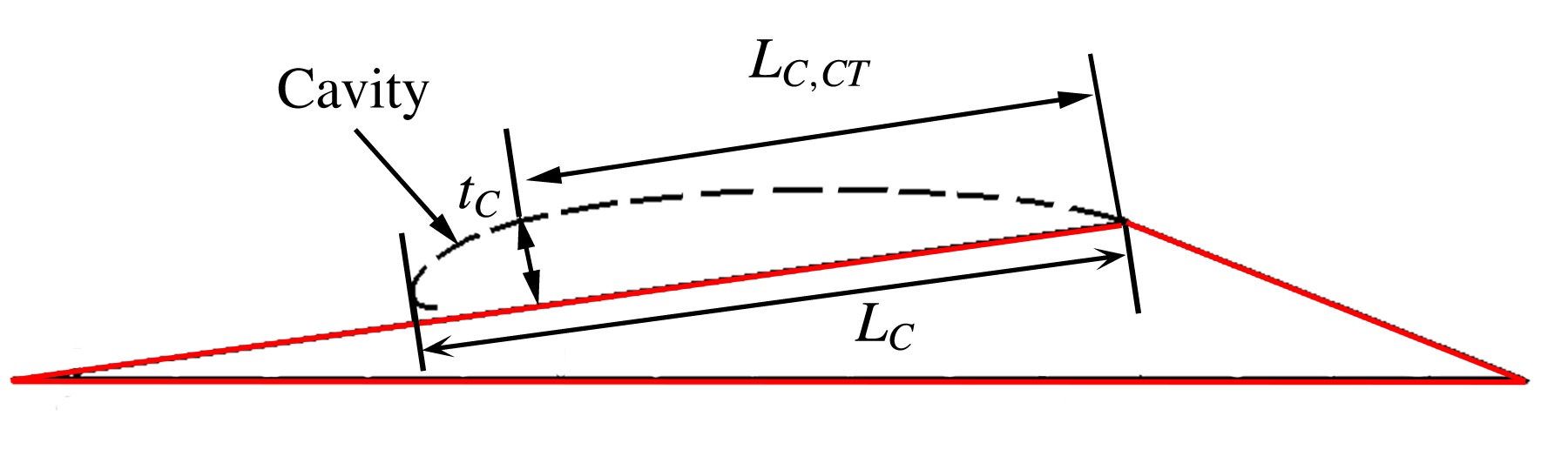
The cavity length increases with decreasing cavitation number. We compare the overall cavity length
 $L_{C}$
, the length of the cavity at the point of its maximum thickness
 $L_{CT}$
and the maximum thickness
 $t_{C}$
, predicted from the analytical solution with the experimental observations from high-speed videos and X-ray measurements. For the estimation of cavity lengths from high-speed videos, only side view videos were used. Both the lengths were measured along the surface of the wedge parallel to the
 $s$
direction and thickness normal to the surface of the wedge in the
 $n$
direction, as shown in figure 2. These lengths are normalized by the length of the wedge aft of the apex,
 $L_{W}$
. Figure 5 shows a schematic of the cavity and length definitions.
The dimensions of the cavity where
 $L_{C}$
is the average cavity length,
 $L_{CT}$
is the length to the position of maximum cavity thickness and
 $t_{C}$
is the maximum cavity thickness. For periodically shedding cavities the maximum cavity length is defined as
 $L_{CM}$
.

The average length,
 $L_{C}$
, and thickness,
 $t_{C}$
, of the cavities were determined by inspection of the high-speed video images. With the aid of the markings on the wedge surface spaced 10 mm apart, the length of the cavity from the top and side views were measured. For shedding cavities, the maximum cavity length for a given cycle was measured and averaged over several cycles to obtain the final cavity length at a given cavitation number. In addition, the cavity dimensions can also be measured using the X-ray densitometry system. For incipient and transitional cavities, contour lines corresponding to
 $\langle \unicode[STIX]{x1D6FC}\rangle =0.05$
void fraction in time-averaged void-fraction flow field measurements were used to designate cavity length. Maximum cavity thickness was obtained by measuring the perpendicular distance between the location of maximum thickness and the wedge surface. The cavity length corresponding to the location of maximum thickness,
 $L_{CT}$
, was also measured. For shedding cavities, the maximum cavity length for a given cycle,
 $L_{CM}$
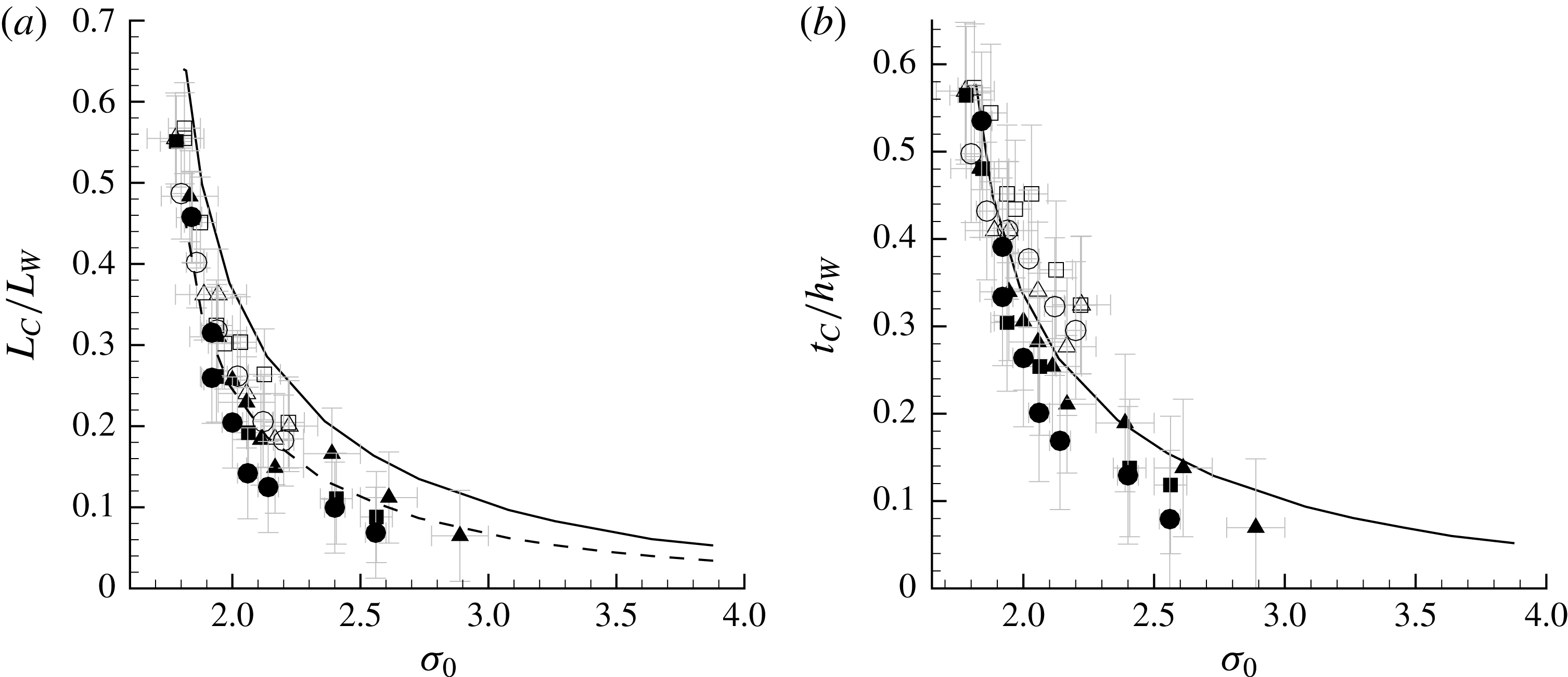
, was used as the cavity length. The variation of cavity length and thickness from different measurements with cavitation number are shown in figure 6(a) and 6(b), respectively. The measured values are also compared with cavity dimensions obtained from the analytical model. There is no observable inlet speed dependence on both cavity length and thickness.
Variation of (a) average cavity length,
 $L_{C}/L_{W}$
, and (b) maximum cavity thickness,
 $t_{C}/h_{W}$
, with cavitation number,
 $\unicode[STIX]{x1D70E}_{0}$
, for three inlet speeds
 $U_{0}=6~\text{m}~\text{s}^{-1}$
(▴), 8 m s
 $^{-1}$
(▪) and 10 m s
 $^{-1}$
(●). The open symbols are measurements from the video images and the filled symbols are from the X-ray images. For periodically shedding cavities (
 $\unicode[STIX]{x1D70E}_{0}<1.9$
), the maximum cavity length
 $L_{CM}/L_{W}$
is plotted. Also shown in (a) are the solution from the free-streamline theory for the cavity length (solid line) and the length to the point of maximum cavity thickness (dashed line); the solution for the maximum cavity thickness is shown in (b).

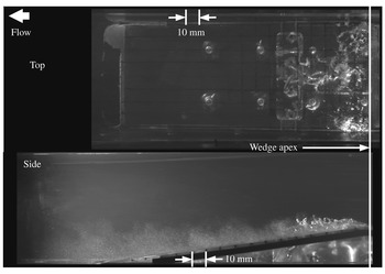
High-speed video snapshot of an incipient cavity forming on the wedge;
 $\unicode[STIX]{x1D70E}_{0}=2.46$
,
 $U_{0}=8~\text{m}~\text{s}^{-1}\times 10~\text{mm}$
corresponds to
 $x/L_{W}=0.06$
.

The analytical solution predicts a higher inception cavitation number,
 $\unicode[STIX]{x1D70E}_{i}$
, compared to the experimentally observed value,
 $\unicode[STIX]{x1D70E}_{0i}$
, where
 $\unicode[STIX]{x1D70E}_{i}\approx \unicode[STIX]{x1D70E}_{0i}+0.23$
. The experimentally observed cavity lengths generally matched the cavity length corresponding to the position of the maximum thickness from the analytical solution
 $L_{CM}$
, as shown by the dotted line in figure 6(b). The overall cavity length obtained from the analytical solution is longer than the experimentally observed cavity length for stable (non-shedding) cavities. This trend is similar to that observed by Laberteaux & Ceccio (Reference Laberteaux and Ceccio2001a
) for stable open cavities. In both studies, the incipient and transitional cavities would terminate at or near the position of maximum cavity thickness, suggesting that the pressure recovery in the closure reason arrested the cavity growth. However, the maximum length,
 $L_{CM}$
, observed for the shedding cavities during a given filling and shedding cycle closely matched the analytically predicted cavity length for the same cavitation number, without correction.
4.2 The incipient cavity
Figure 7 shows a still image from a high-speed video of incipient partial cavitation taken from the top and side view of the wedge at
 $\unicode[STIX]{x1D70E}_{0}=2.46$
at
 $U_{0}=8~\text{m}~\text{s}^{-1}$
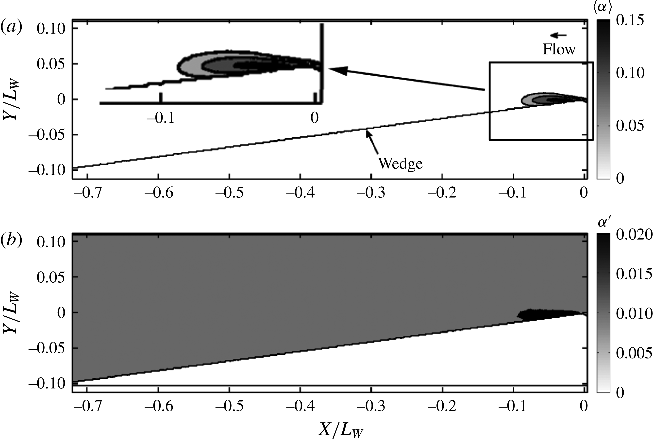
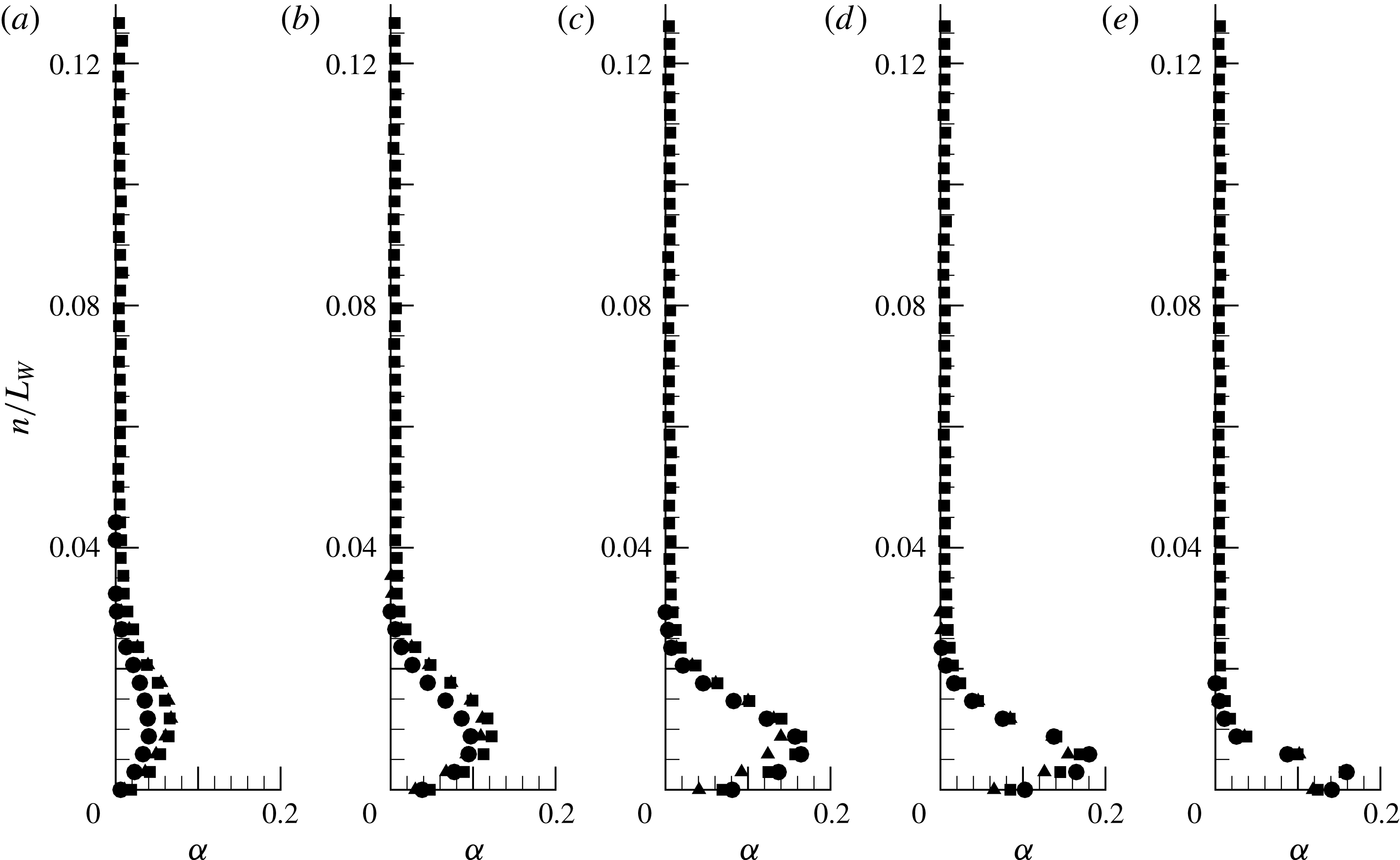
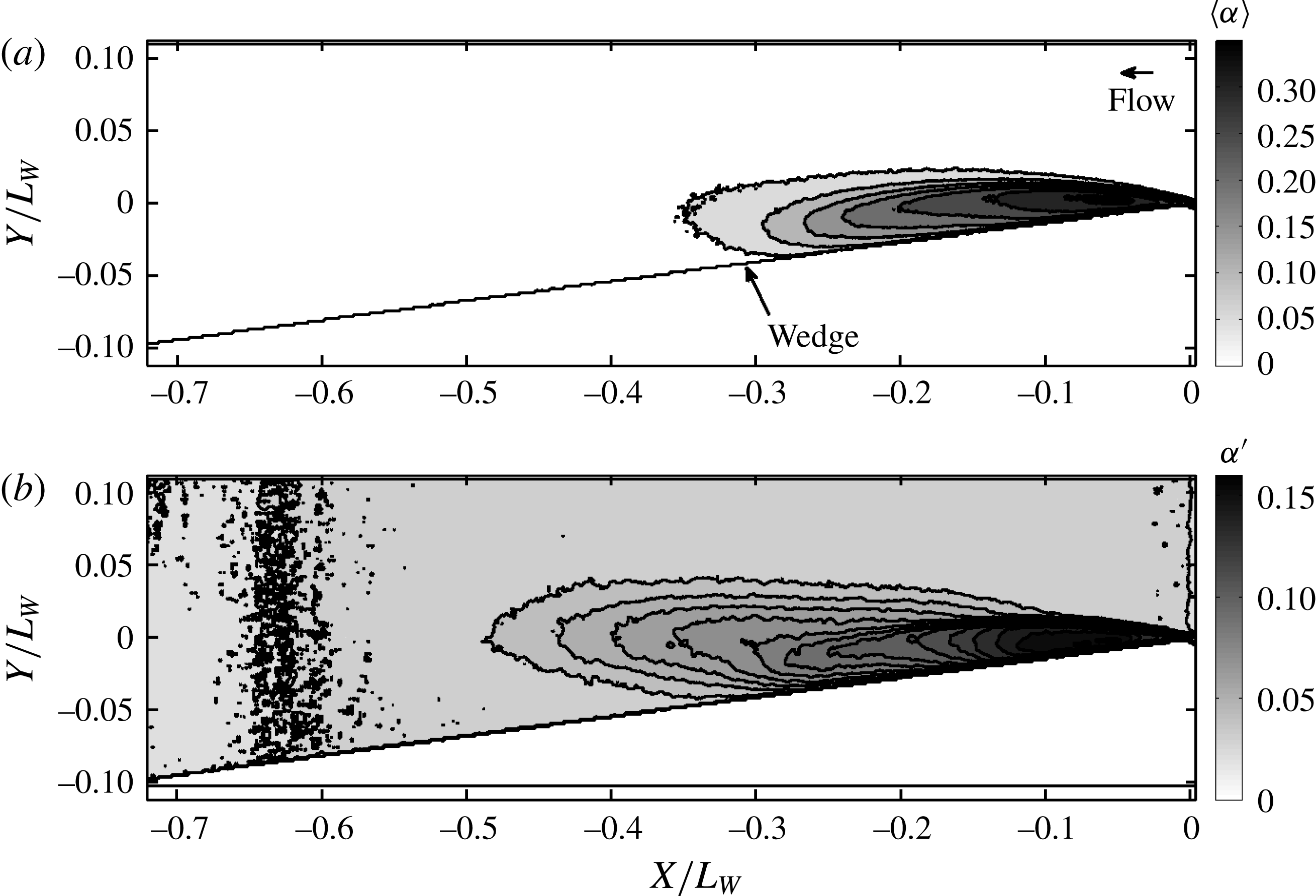
. The cavity is not a gas pocket, as hypothesized in the analytical model. Instead, it is a low void-fraction bubbly mixture. X-ray densitometry-based void-fraction measurements of the incipient cavity were also conducted at the same flow conditions. Figures 8(a) and 8(b) show
 $\langle \unicode[STIX]{x1D6FC}\rangle$
and
 $\unicode[STIX]{x1D6FC}^{\prime }$
of the void-fraction flow field. In addition to field measurements, void-fraction profiles in the wall-normal direction
 $n$
of the wedge at different locations
 $s$
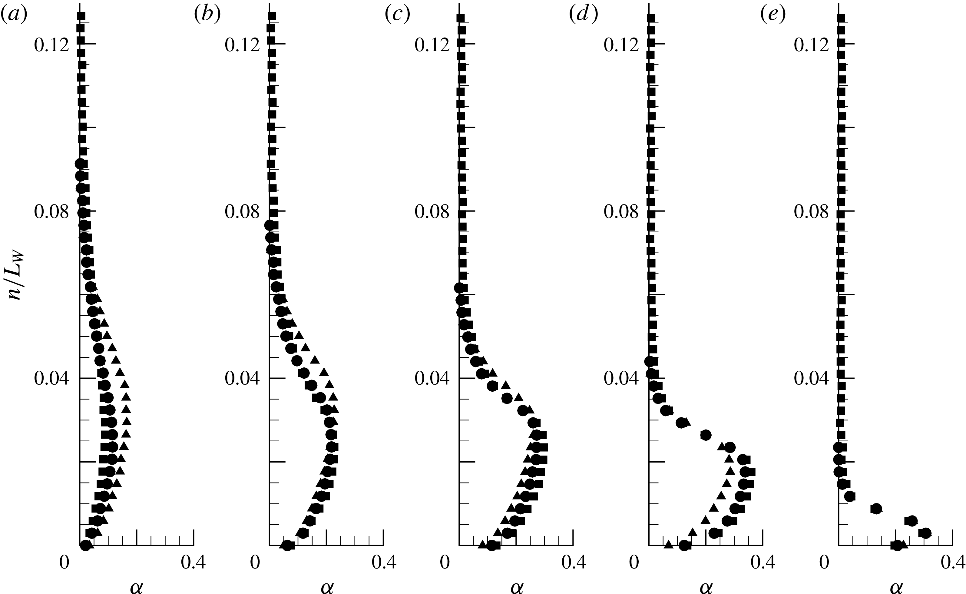
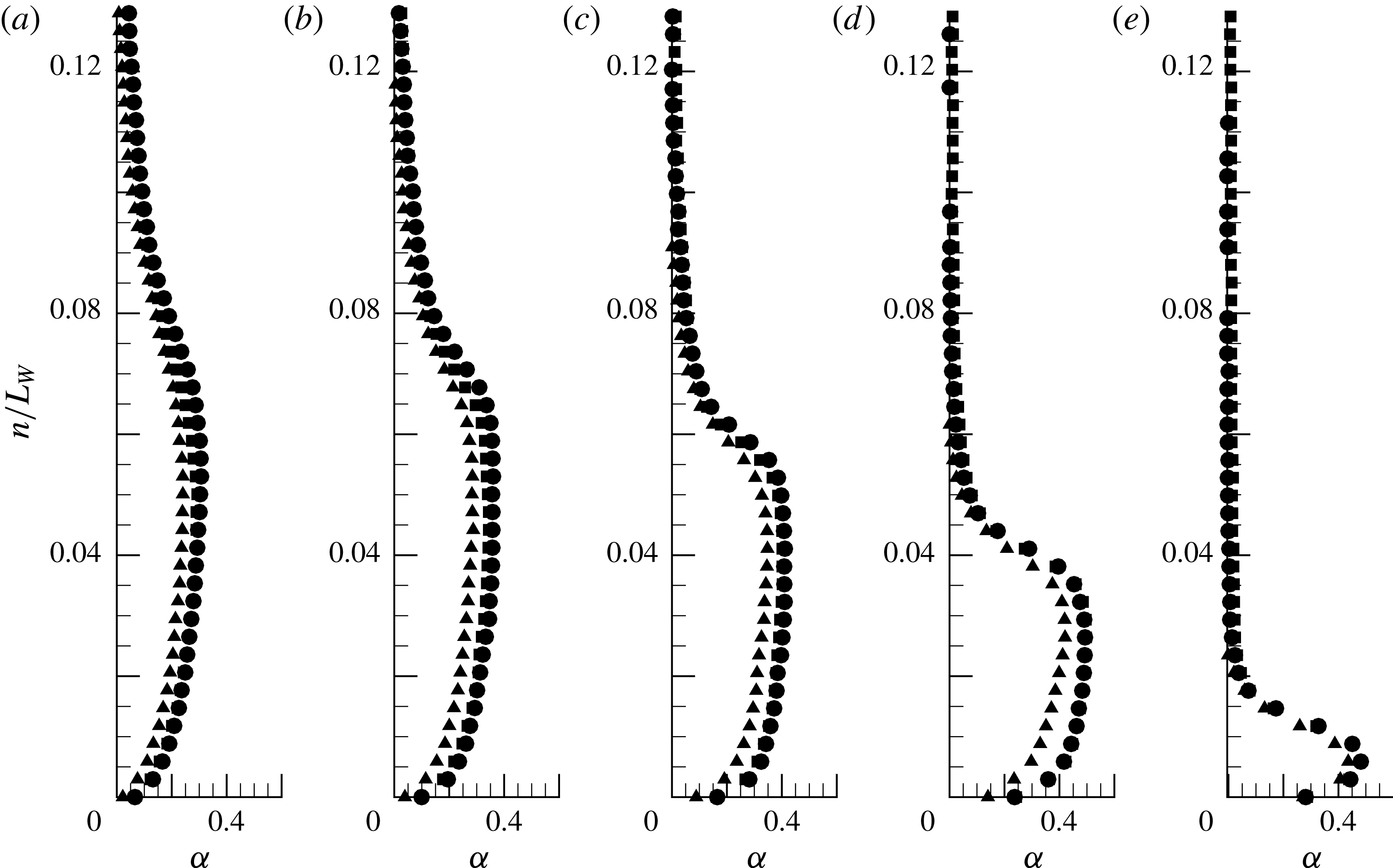
along the wedge length are shown in figure 9. The local average void fraction is highest near the wedge apex, and within the cavity the void fraction is highest near the cavity mid-thickness. Note that changes in the flow speed did not lead to dramatic changes in the void-fraction profile. (However, when considering the absolute void-fraction values, especially with the small incipient cavities, we need to be mindful of the increased measurement uncertainty, particularly near the apex, due to non-parallel beam paths and other limitations of the measurement system as discussed by Mäkiharju (Reference Mäkiharju2012).)
X-ray densitometry-based void-fraction field for incipient cavity; (a) the mean void fraction
 $\langle \unicode[STIX]{x1D6FC}\rangle$
, (b) the fluctuations
 $\unicode[STIX]{x1D6FC}^{\prime }$
for
 $\unicode[STIX]{x1D70E}_{0}=2.41$
at
 $U_{0}=8~\text{m}~\text{s}^{-1}$
. The top left corner of (a) shows the zoomed picture of the rectangular area.

Surface-normal profile of
 $\langle \unicode[STIX]{x1D6FC}\rangle$
for the incipient cavity at locations
 $s/L_{W}=0.1$
, 0.08, 0.06, 0.04 and 0.02 (a–e) for three free-stream speeds for
 $\unicode[STIX]{x1D70E}_{0}=2.41$
and
 $U_{0}=6~\text{m}~\text{s}^{-1}$
(▴), 8 m s
 $^{-1}$
(▪) and 10 m s
 $^{-1}$
(●).

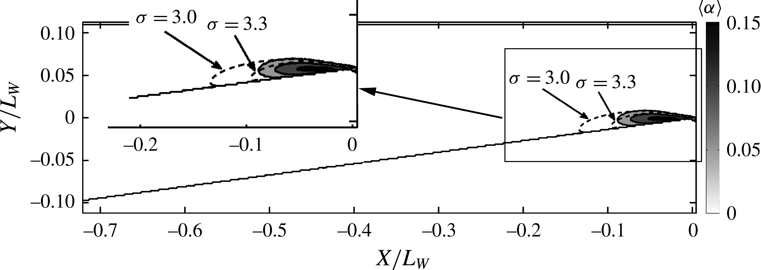
Free-streamline solution for
 $\unicode[STIX]{x1D70E}=3.0$
and 3.3 compared to the measured mean void-fraction flow field from X-ray densitometry
 $\langle \unicode[STIX]{x1D6FC}\rangle$
for the incipient cavity for
 $\unicode[STIX]{x1D70E}_{0}=2.41$
and
 $U_{0}=8~\text{m}~\text{s}^{-1}$
. The top left corner shows the zoomed picture of the rectangular area.

Figure 10 presents an overlay of the free-streamline-theory-based cavity shape on the averaged void-fraction flow field, and this illustrates how the free-streamline solution compares with the measured time-averaged void-fraction profiles. The isoline represented by
 $\langle \unicode[STIX]{x1D6FC}\rangle =0.05$
lies outside the predicted cavity shape in the middle and aft portion of the cavity for
 $\unicode[STIX]{x1D70E}=3.3$
, while it was well contained for the cavity shape predicted at
 $\unicode[STIX]{x1D70E}=3.0$
. The best match lies somewhere between these two cavitation numbers, which is consistent with the difference in inception cavitation numbers discussed above. The solutions approximately match until the point of maximum thickness.
4.3 The transitional cavity
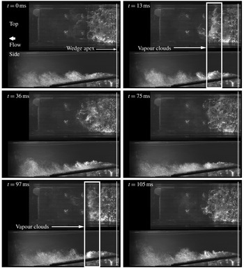
With a further reduction in cavitation number, an incipient cavity of stable length began to exhibit intermittent variation of the cavity length of the order of 30 % of the mean cavity length. Images of a transitional cavity obtained using high-speed video are shown in figure 11. The inlet cavitation number corresponds to a value of
 $\unicode[STIX]{x1D70E}_{0}=2.06$
with
 $U_{0}=8~\text{m}~\text{s}^{-1}$
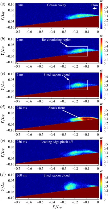
. The vapour clouds that often rolled up in the latter portion of the cavity are highlighted. These clouds separate from the main cavity approximately one-half to two-thirds of the cavity length downstream from the wedge apex. However, sometimes large clouds could be shed from the wedge apex. The time series from the X-ray imaging system revealed two different mechanisms associated with this shedding, as shown in figure 12. One corresponds to a re-circulating vapour cloud that is shed from the aft portion of the cavity. This was also observed in the high-speed video. From the flow fields at 2 and 5 ms one can infer the presence of flow structure that flows beneath the cavity and leads to the pinch off of a vapour pocket. In this case, the re-entrant liquid flow thickness underneath the cavity is thinner than the cavity thickness. The second mechanism is associated with the propagation of a void-fraction discontinuity. In this case, the propagating discontinuity travels upstream until it impinges on the outer cavity flow near the separation line at the wedge apex, causing leading edge pinch off and cloud shedding. When this mechanism occurs, the cloud is formed at the apex (rather than near the middle of the cavity length), such that a much larger portion of the cavity is shed compare to the re-entrant mechanism. The thickness of the propagating discontinuity is equal to the thickness of the cavity.
High-speed video time series of a transitory cavity forming on the wedge for
 $\unicode[STIX]{x1D70E}_{0}=2.06$
,
 $U_{0}=8~\text{m}~\text{s}^{-1}$
.

Time series of instantaneous X-ray densitometry void-fraction fields of the transitory cavity for
 $\unicode[STIX]{x1D70E}_{0}=2.06$
and
 $U_{0}=8~\text{m}~\text{s}^{-1}$
. Two different types of shedding mechanisms, re-entrant-liquid-flow-induced shedding and bubbly shock-propagation-induced shedding are shown in (a–c) and (d–f), respectively. Both these mechanisms were observed in the same X-ray recording. Time of occurrence is shown in the top right corner of individual pictures. There was no observed periodicity between the mechanisms. Videos are provided as supplementary material available at http://dx.doi.org/10.1017/jfm.2016.425. See movie 1 for figure 8, movies 2 and 3 for figure 12 (movie 3 is another realization of a transitory cavity) and movie 4 for figure 17.

Figure 13 shows
 $\langle \unicode[STIX]{x1D6FC}\rangle$
and
 $\unicode[STIX]{x1D6FC}^{\prime }$
for the transitional cavity. Note that the averaged void-fraction contour has spread in the aft portion of the cavity, and this is a consequence of averaging over many cycles of cavity shedding where the clouds lift up and convect downstream. The
 $\unicode[STIX]{x1D6FC}^{\prime }$
has higher values of void-fraction fluctuation in the regions outside the actual cavity for the same reason. The average void fractions in wall-normal direction at different locations along the wedge are shown in figure 14. For the transitional cavity, the free-stream speed does not exhibit a dominant effect on
 $\langle \unicode[STIX]{x1D6FC}\rangle$
and
 $\unicode[STIX]{x1D6FC}^{\prime }$
.
X-ray densitometry-based void-fraction field for transient cavity in grey scale; (a) the mean void fraction
 $\langle \unicode[STIX]{x1D6FC}\rangle$
, (b) the fluctuations
 $\unicode[STIX]{x1D6FC}^{\prime }$
for
 $\unicode[STIX]{x1D70E}_{0}=2.06$
at
 $U_{0}=8~\text{m}~\text{s}^{-1}$
.

Surface-normal profile of
 $\langle \unicode[STIX]{x1D6FC}\rangle$
for the transitional cavity at locations
 $s/L_{W}=0.29$
, 0.22, 0.15, 0.09 and 0.02 (a–e) for
 $\unicode[STIX]{x1D70E}_{0}=2.06$
and three free-stream speeds
 $U_{0}=6~\text{m}~\text{s}^{-1}$
(▴), 8 m s
 $^{-1}$
(▪) and 10 m s
 $^{-1}$
(●).

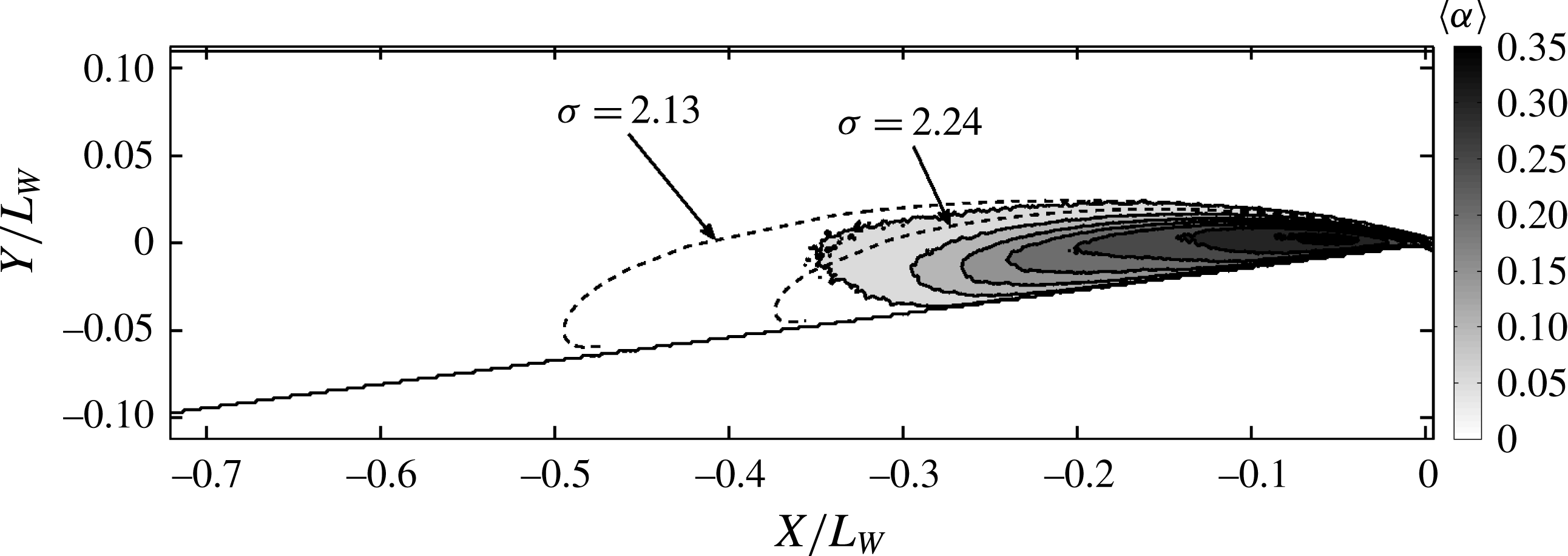
Free-streamline solution for
 $\unicode[STIX]{x1D70E}=2.24$
and 2.13 compared to the measured X-ray densitometry-based mean void-fraction flow field
 $\langle \unicode[STIX]{x1D6FC}\rangle$
for the transient cavity for
 $\unicode[STIX]{x1D70E}_{0}=2.06$
and
 $U_{0}=8~\text{m}~\text{s}^{-1}$
.

A comparison of the analytically obtained cavity shape with experiments is shown in figure 15 for
 $\unicode[STIX]{x1D70E}_{0}=2.06$
, and once again the analytical shape is in good agreement with the time-averaged cavity profile up to the position of maximum cavity thickness. Two analytical shapes corresponding to
 $\unicode[STIX]{x1D70E}=2.24$
and
 $\unicode[STIX]{x1D70E}=2.13$
are also shown. The match between analytical and observed cavity shape improves with decreasing cavitation number.
4.4 The periodically shedding cavity
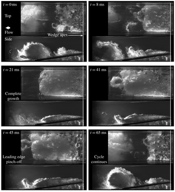
With a further reduction in cavitation number, the large-scale shedding of the cloud cavitation from the wedge apex becomes more prominent and periodic. Figure 16 shows images from a high-speed video of a periodically shedding cavity at a free-stream cavitation number of
 $\unicode[STIX]{x1D70E}_{0}=1.95$
and
 $U_{0}=8~\text{m}~\text{s}^{-1}.$
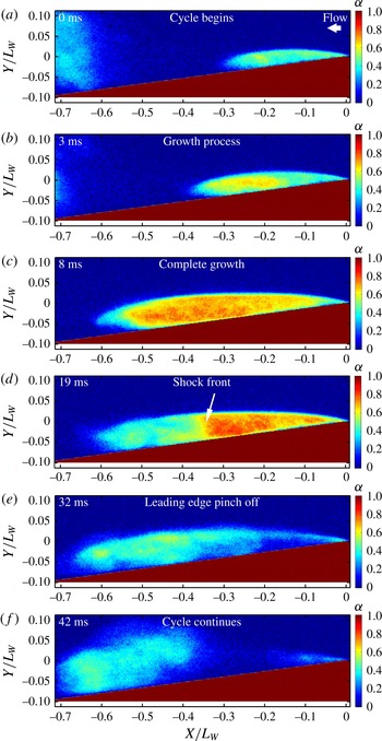
The cavity exhibits well defined and periodic growth and collapse cycles, and shedding is produced by leading edge pinch off of the cavity. The cloud cavity that is shed convects up and away from the cavity after pinch off. For this periodically shedding cavity, the propagation of a front in the cavity void fraction is well defined for most of the cycles, as shown in figure 17. The front is evident in this measurement representing the spanwise average of the cavity void fraction, and lies perpendicular to the solid surface beneath the cavity and the cavity interface. For some cycles, however, the shock front seen in this spanwise-average measurement is less distinct, which could be due to variations in the spanwise direction. The void fraction upstream of the front is significantly higher than that downstream.
High-speed video time series of images of the periodically shedding cavity taken for
 $\unicode[STIX]{x1D70E}_{0}=1.95$
and
 $U_{0}=8~\text{m}~\text{s}^{-1}$
. The images show the growth, pinch off and shedding of a large vapour cloud from the cavity near the separation line at the wedge apex.

Time series of X-ray densitometry-based void-fraction fields of the periodically shedding cavity for
 $\unicode[STIX]{x1D70E}_{0}=1.95$
and
 $U_{0}=8~\text{m}~\text{s}^{-1}$
. The shedding process resulting from the propagation of a front in void fraction is shown.

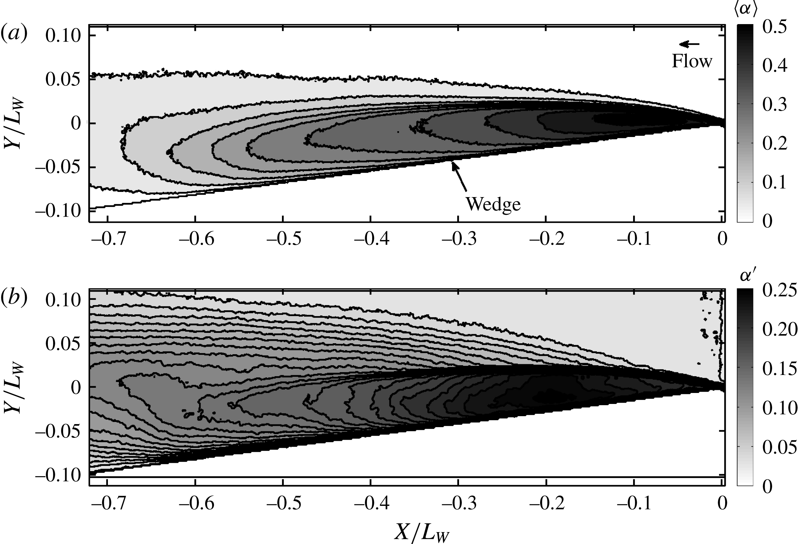
X-ray densitometry-based void-fraction field for periodically shedding cavity in grey scale; (a) the mean void fraction
 $\langle \unicode[STIX]{x1D6FC}\rangle$
, (b) the fluctuations
 $\unicode[STIX]{x1D6FC}^{\prime }$
for
 $\unicode[STIX]{x1D70E}_{0}=1.95$
and
 $U_{0}=8~\text{m}~\text{s}^{-1}$
.

Surface-normal profile of
 $\langle \unicode[STIX]{x1D6FC}\rangle$
for the periodically shedding cavity at locations
 $s/L_{W}=0.49$
, 0.37, 0.26, 0.14 and 0.02 (a–e) for
 $\unicode[STIX]{x1D70E}_{0}=1.95$
and three free-stream speeds
 $U_{0}=6~\text{m}~\text{s}^{-1}$
(▴), 8 m s
 $^{-1}$
(▪) and 10 m s
 $^{-1}$
(●).

Free-streamline solution for
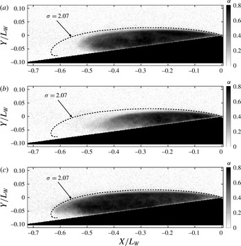
 $\unicode[STIX]{x1D70E}=2.07$
compared to three instantaneous images of the void-fraction field
 $\unicode[STIX]{x1D6FC}$
based on X-ray densitometry for periodically shedding cavity for
 $\unicode[STIX]{x1D70E}_{0}=1.95$
and
 $U_{0}=8~\text{m}~\text{s}^{-1}$
.

Fields of
 $\langle \unicode[STIX]{x1D6FC}\rangle$
and
 $\unicode[STIX]{x1D6FC}^{\prime }$
for the periodic cavity are shown in figure 18(a,b) and section profiles are shown in 19(a,b) at different locations along the streamwise direction. Again, there is no observable dependence of inlet speed on mean and standard deviation of void fraction along the wall-normal direction. Analytical solutions for the cavity profiles were compared with instantaneous cavity profiles obtained from X-ray measurements. Figure 20(a–c) illustrates this for a cavity exhibiting periodic shedding. When the cavity reaches it maximum length, the profile closely resembles that of the analytical solution, including a portion of the profile downstream of the point of maximum cavity thickness.
4.5 Cloud shedding mechanisms
Examination of both the video and void-fraction time series reveal two basic processes that lead to large-scale shedding of vapour at the cavity trailing edge. The first is the classically described re-entrant flow of liquid at the cavity closure. This mechanism was mainly observed for transitional cavities. With re-entrant shedding, a mostly liquid flow, with thickness a fraction that of the cavity thickness, moves upstream beneath the cavity from the location of cavity closure, leading to a pinch off of a portion (usually cavity contents from closure up to its mid-length). Figure 12(a–c) represents a re-entrant flow mechanism. Such a mechanism results from the kinematics of a separated flow sustaining a constant pressure cavity and the presence of a stagnation line roughly parallel to the nominally two-dimensional line of the cavity closure. However, when the cavitation number is reduced and the void fraction in the cavity increases, a second process begins to dominate the shedding process. Under these conditions, a well-defined void-fraction front is often discerned that spans the thickness of the cavity, and this front propagates upstream with a speed that is slower than the speed of the liquid flow outside of the cavity interface. When the discontinuity in void fraction reaches the region of cavity detachment at the wedge apex, a large vapour cloud is shed. This is illustrated in figure 17(a–f). We will refer to this as shock-wave-induced shedding. The incipient cavities did not produce large-scale shedding, while transitional cavities could exhibit both re-entrant and shock-wave-induced shedding. The periodically shedding cavities in the present geometry were dominated by the shock-wave shedding mechanism.
4.6 Cavity shedding frequency and Strouhal number
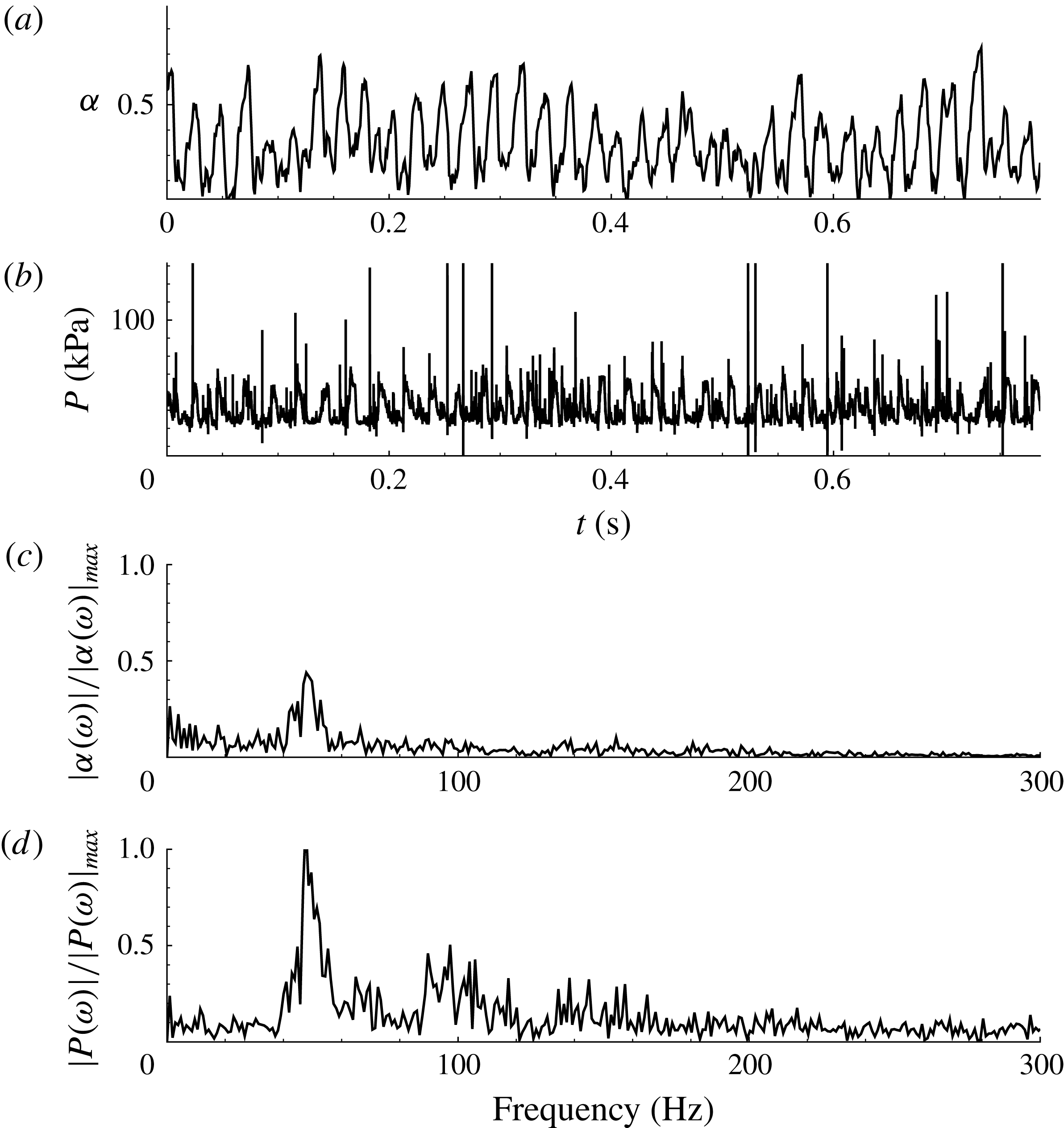
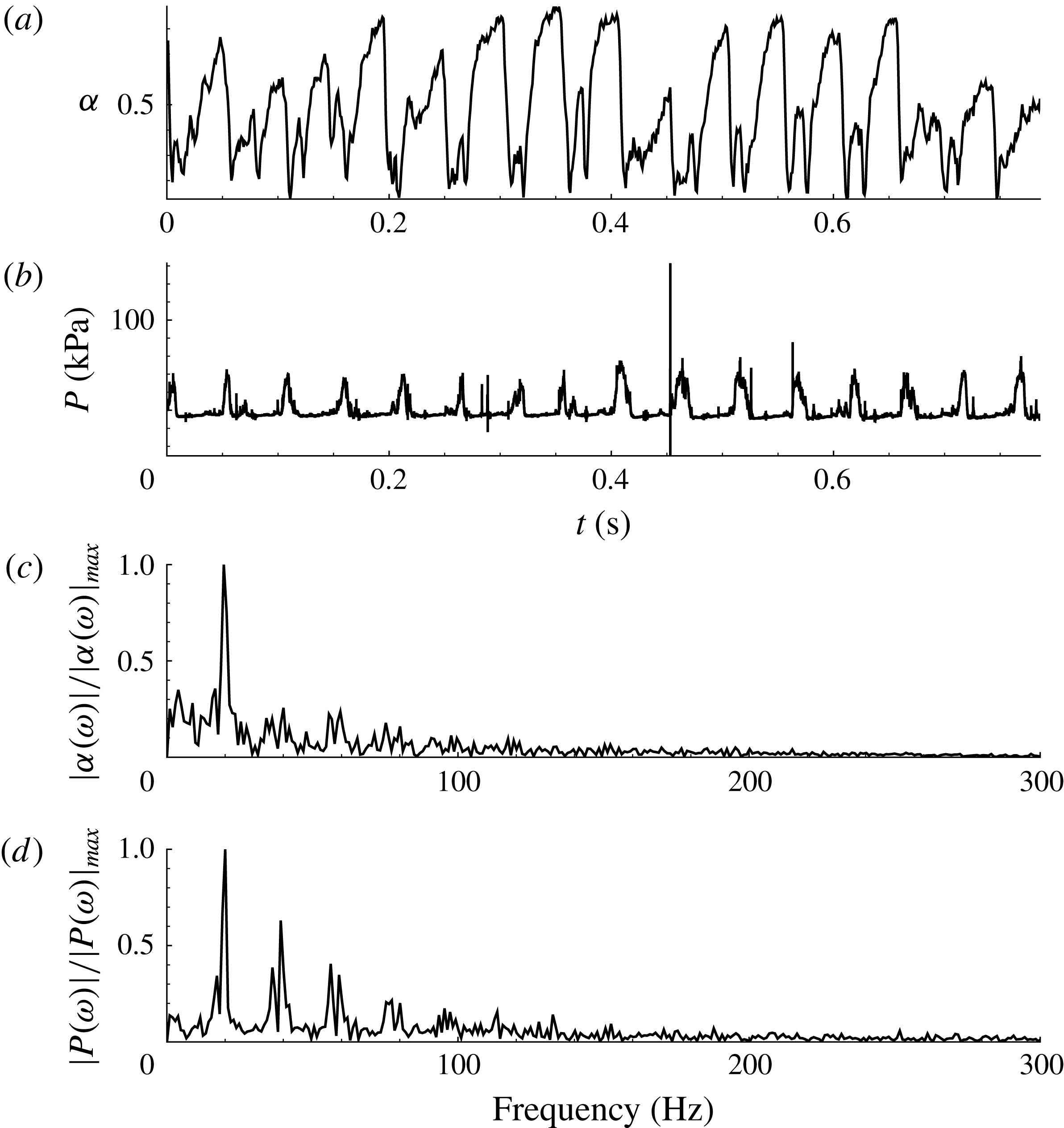
Unsteadiness in a periodic cavity can be characterized by the time-varying cavity void fraction at a given location within the cavity and by the time-varying surface pressure beneath the cavity. The time varying void fraction was examined at a position near the apex of the wedge, VF, as shown in figure 2(b). A sample time trace of the local void fraction and dynamic pressure at DP2 are shown in figure 21(a,b) for the transitory cavity and figure 22(a,b) for a shedding cavity. The normalized fast Fourier transforms (FFT) of these signals are shown in (c,d). For the shedding cavity signals shown in (figure 22), FFT of both void fraction and pressure signal reveal the presence of dominant frequencies at approximately 20 Hz, with smaller peaks or harmonics at 40 and 60 Hz. This is consistent with the observed vapour production and shedding period obtained through videography, and the dominant spectral peaks are consistent between the pressure and void-fraction time traces. The strongly shedding case has a much sharper spectral peak compared to the transitory case, consistent with its observed periodicity.
Time traces of the (a) void fraction and (b) dynamic pressure signal for the transitional cavity; the normalized FFT of the signals is shown in (c) and (d) for
 $\unicode[STIX]{x1D70E}_{0}=2.03$
and
 $U_{0}=8~\text{m}~\text{s}^{-1}$
.

Time traces of the (a) void fraction and (b) dynamic pressure signal for the periodically shedding cavity; the normalized FFT of the signals is shown in (c) and (d) for
 $\unicode[STIX]{x1D70E}_{0}=1.95$
and
 $U_{0}=8~\text{m}~\text{s}^{-1}$
.

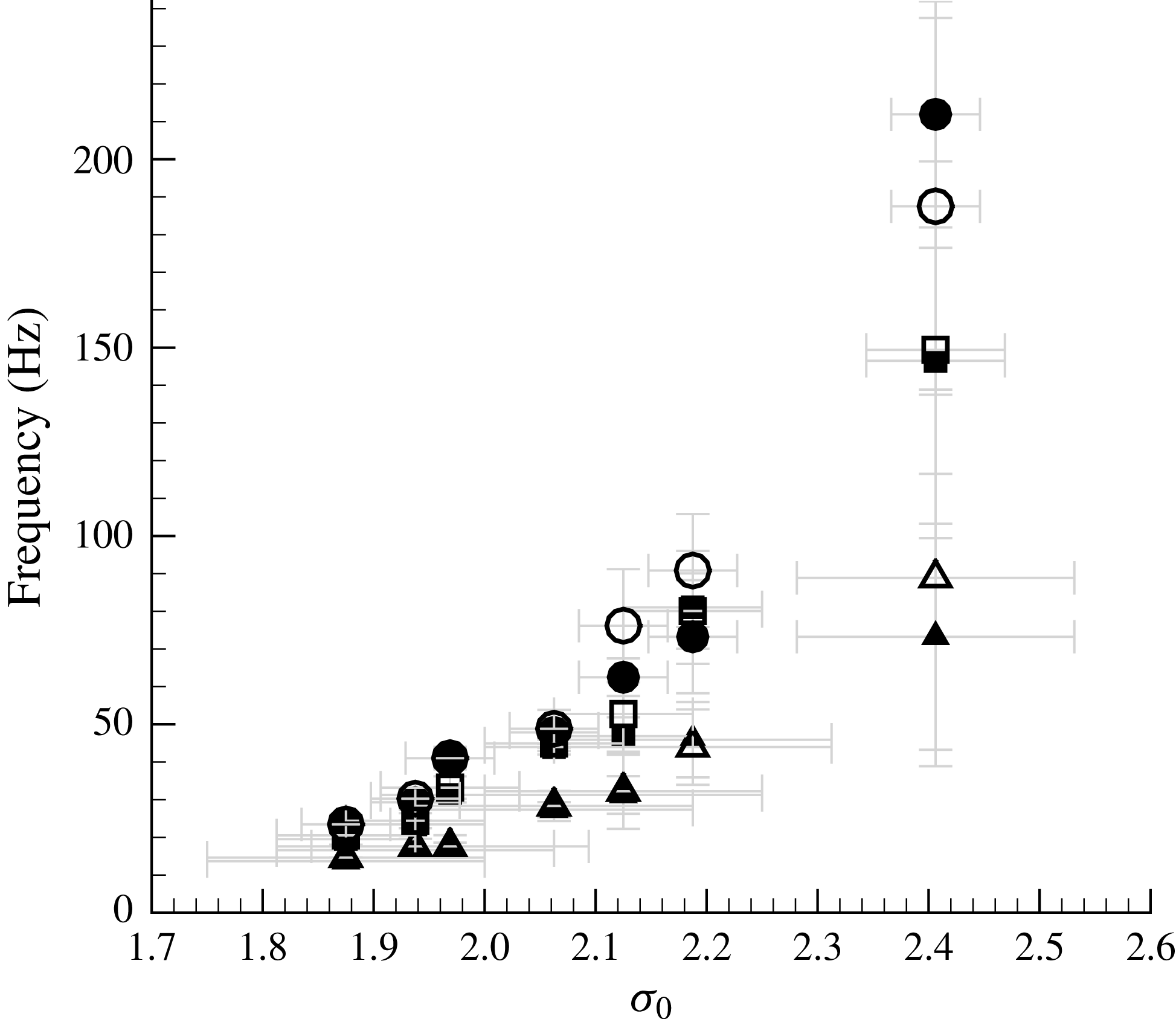
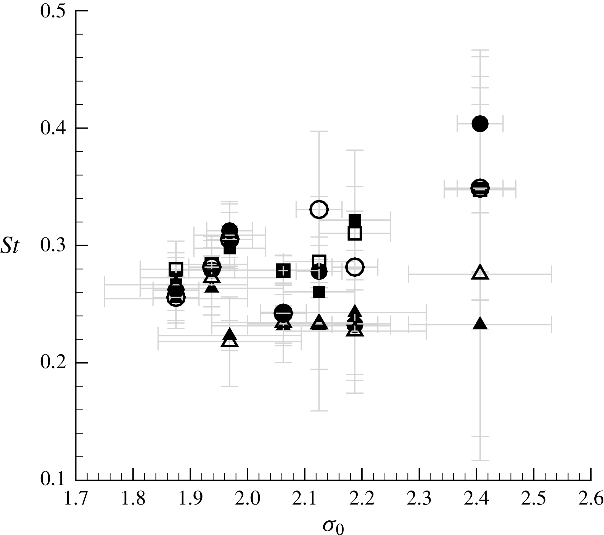
The most dominant frequency based on measurements of both pressure and void fraction are plotted in figure 23 as a function of cavitation number. At higher cavitation numbers, the void fraction and dynamic pressure principal frequencies do not match, suggesting little correlation between pressure fluctuations and the cavity vapour dynamics. But, with a reduction in cavitation number, both these frequencies begin to converge until they essentially match for the periodically shedding cavities, indicating that the cloud shedding mechanism associated with the propagation of the void-fraction front dominates the cavity dynamics. The shedding frequency is higher for higher flow speeds, which suggests the dependence of shock propagation speed on the inlet speed.
The measured dominant frequency,
 $f$
, with cavitation number,
 $\unicode[STIX]{x1D70E}_{0}$
, for three inlet speeds
 $U_{0}=6~\text{m}~\text{s}^{-1}$
(▴), 8 m s
 $^{-1}$
(▪) and 10 m s
 $^{-1}$
(●). The open symbols are data from the pressure measurements and the closed symbols are from the void-fraction measurements.

Strouhal number,
 $St$
, for varying cavitation number,
 $\unicode[STIX]{x1D70E}_{0}$
, for three inlet speeds
 $U_{0}=6~\text{m}~\text{s}^{-1}$
(▴), 8 m s
 $^{-1}$
(▪) and 10 m s
 $^{-1}$
(●). The open symbols are data from the pressure measurements and the closed symbols are from the void-fraction measurements.

Figure 24 presents the Strouhal number as a function of cavitation number for both the void-fraction and pressure time signals. The Strouhal number
 $St$
is defined as,
 $$\begin{eqnarray}\displaystyle St=\frac{fL_{S}}{U_{0}}. & & \displaystyle\end{eqnarray}$$
In this case,
 $f$
represents the dominant frequency and
 $L_{S}$
represents a length scale that depends on the cavity topology. For the case of incipient and transitional cavities, the characteristic length is chosen to be the mean cavity length
 $L_{S}=L_{C}$
and for periodically shedding cavities,
 $L_{S}=L_{CM}$
, the averaged maximum cavity length in a given cycle, is chosen. For the periodically shedding conditions,
 $St\approx 0.26\pm 0.02$
, which is consistent with the value of
 $St=0.28$
reported by Stutz & Legoupil (Reference Stutz and Legoupil2003). Based on the wedge blockage ratio
 $\unicode[STIX]{x1D706}$
, the average velocity of the flow over the cavity is
 ${\sim}U_{0}/(1-\unicode[STIX]{x1D706})=3/2U_{0}$
, and we can use this together with
 $L_{CM}$
to estimate the Strouhal number a periodic cavity shedding cycle that consists of a three steps: cavity filling, convection of a disturbance upstream to the cavity apex (re-entrant jet or condensation shock) and cavity shedding (advection of a vapour cloud downstream). Then, the shedding frequency could at most be approximately
 $f_{M}=1/3\times 3/2U_{0}/L_{CM}$
, yielding
 $St_{M}=1/2$
. This is an upper bound, as the speed at the cavity interface will be less than the throat speed. However, for incipient and transitional cavities, the Strouhal numbers span a wider range. Strouhal number values converge for different speeds for well-defined periodicity. This suggests the importance of the ratio of time scales involved the observed dynamics.
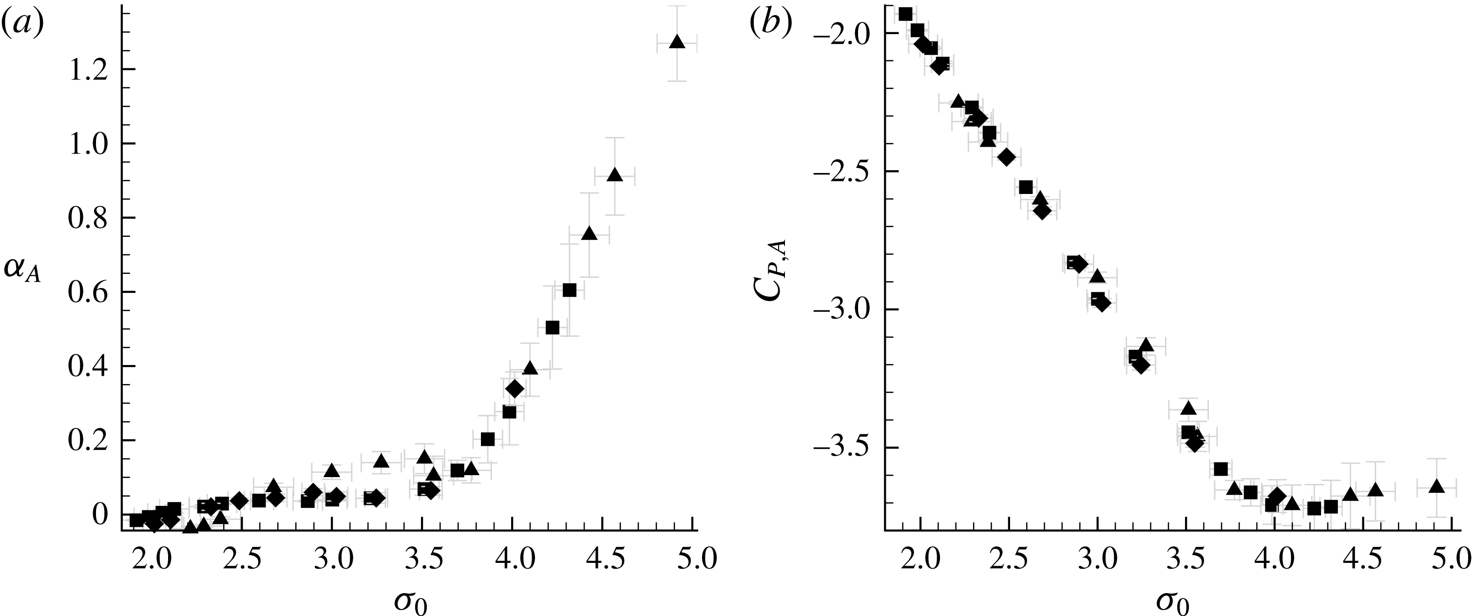
The average apex cavitation number,
 $\unicode[STIX]{x1D70E}_{A}$
, and pressure coefficient,
 $C_{PA}$
, as a function of the inlet cavitation number
 $\unicode[STIX]{x1D70E}_{0}$
for three inlet speeds
 $U_{0}=6~\text{m}~\text{s}^{-1}$
(▴), 7 m s
 $^{-1}$
(♦) and 8 m s
 $^{-1}$
(▪).

4.7 The average pressure under the cavity
The static pressure under the cavity was measured using pressure taps A and D on the wedge surface, as shown in figure 2(b). The average pressure at the apex of the wedge,
 $p_{A}$
, was measured for different cavitation numbers and inlet flow speeds at tap A. Apex pressure measurements were carried out for inlet speeds corresponding to 6, 7 and 8 m s
 $^{-1}$
. This was done so that the maximum pressure in the test section needed to achieve non-cavitating flow did not exceed the maximum capacity of the facility, which is 200 kPa. Beginning at a high cavitation number that resulted in minimal to no cavitation at the wedge apex, the pressure was gradually reduced until a stable cavity remained attached at the wedge apex. The cavitation number at the apex is defined as
 $$\begin{eqnarray}\displaystyle \unicode[STIX]{x1D70E}_{A}=\frac{(p_{A}-p_{V})}{\frac{1}{2}\unicode[STIX]{x1D70C}U_{0}^{2}}. & & \displaystyle\end{eqnarray}$$
Once the apex pressure reached a value close to the vapour pressure (i.e. at inception),
 $\unicode[STIX]{x1D70E}_{A}$
becomes nearly insensitive to changes in
 $\unicode[STIX]{x1D70E}_{0}$
, as shown in figure 25(a). There is also not a appreciable dependence on inlet flow speed. The pressure coefficient at the apex,
 $C_{PA}$
, is defined as
 $$\begin{eqnarray}\displaystyle C_{PA}=\frac{(p_{A}-p_{0})}{\frac{1}{2}\unicode[STIX]{x1D70C}U_{0}^{2}}. & & \displaystyle\end{eqnarray}$$
Figure 25(b) plots
 $C_{PA}$
versus
 $\unicode[STIX]{x1D70E}_{0}$
, and this shows that the pressure coefficient at the apex is nominally constant at
 $C_{PA}=-3.71$
for the non-cavitating flow. The non-cavitating value of
 $C_{PA}=-3.71$
is significantly lower than the nominal value of
 $C_{PA}=(1-(1-\unicode[STIX]{x1D706})^{-2})=-1.25$
that we would estimate using the average flow speed in the throat due to the blockage of the wedge, indicating that there is a strong local suction peak at the wedge apex. After inception, the apex pressure is nearly equivalent to the vapour pressure with
 $C_{PA}\approx -\unicode[STIX]{x1D70E}_{0}$
.
The average static pressure beneath the cavity and downstream of the apex,
 $p_{D}$
, was measured at the location Tap D. The cavitation number based on
 $p_{D}$
is given by
 $$\begin{eqnarray}\displaystyle \unicode[STIX]{x1D70E}_{D}=\frac{(p_{D}-p_{V})}{\frac{1}{2}\unicode[STIX]{x1D70C}U_{0}^{2}}. & & \displaystyle\end{eqnarray}$$
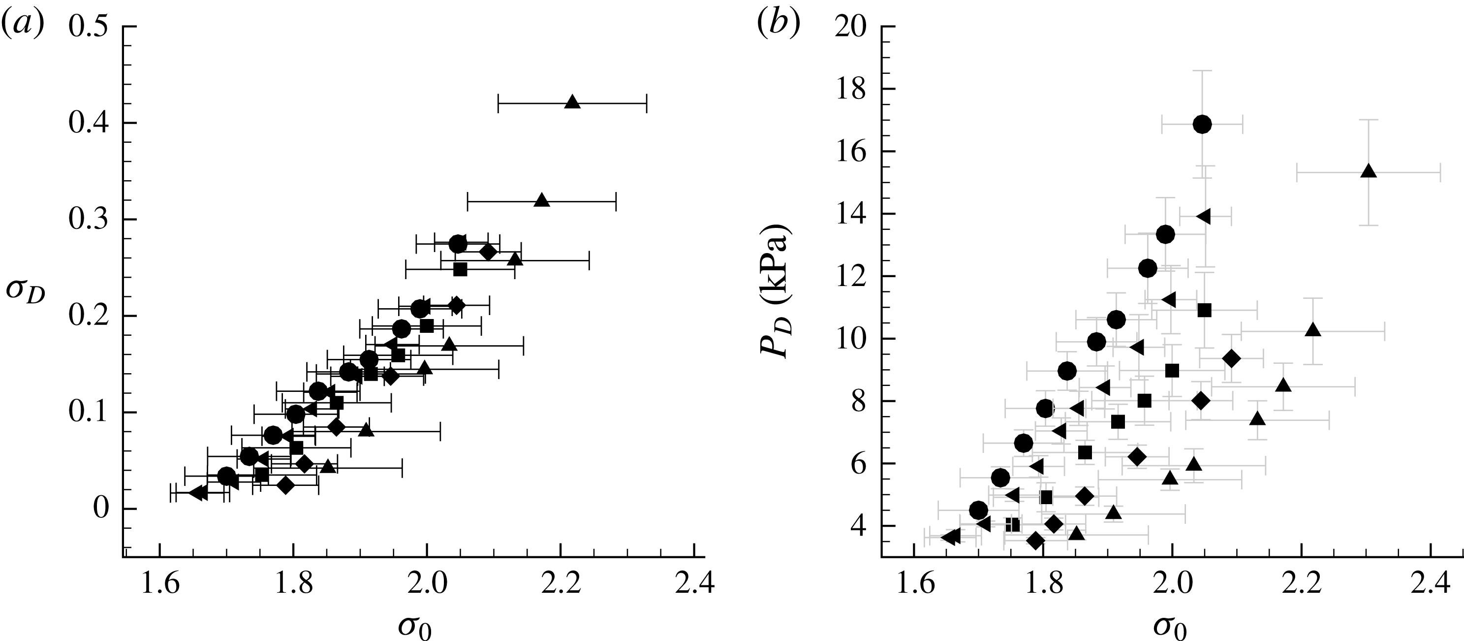
Figure 26(a,b) presents
 $p_{D}$
and
 $\unicode[STIX]{x1D70E}_{D}$
as a function of
 $\unicode[STIX]{x1D70E}_{0}$
, for different speeds. For
 $p_{D}$
measurements, the inlet speed was varied between 6 to 10 m s
 $^{-1}$
. Note that that for shedding cavities, the pressure represents the average cavity pressure over many cycles. In most cases, even for those with high cavity void fraction, the average pressure is higher than the vapour pressure (
 $\unicode[STIX]{x1D70E}_{D}>0$
) and it is also generally higher than the apex pressure (
 $\unicode[STIX]{x1D70E}_{D}>\unicode[STIX]{x1D70E}_{A}$
). These results show that the static pressure in the cavity is not necessarily constant with varying inlet speed and hence inlet pressure, and it is only at vapour pressure very near the wedge apex. On an average the pressure in the cavity at the measurement location
 $D$
is higher as the speed increases for a fixed inlet cavitation number,
 $\unicode[STIX]{x1D70E}_{0}$
. In the next section, we will see how these observations are related to the formation and propagation of a bubbly condensation shock.
The average downstream cavitation number,
 $\unicode[STIX]{x1D70E}_{D}$
, and pressure,
 $P_{D}$
, as a function of the inlet cavitation number
 $\unicode[STIX]{x1D70E}_{0}$
for five inlet speeds
 $U_{0}=6~\text{m}~\text{s}^{-1}$
(▴), 7 m s
 $^{-1}$
(♦), 8 m s
 $^{-1}$
(▪), 9 m s
 $^{-1}$
(◂) and 10 m s
 $^{-1}$
(●).

5 Bubbly shock propagation within the partial cavity
Brennen (Reference Brennen2005) discusses the underlying mechanism of bubbly shock-wave propagation in cavitating flows, including the influence of bubble dynamics. Here we will start with the simplest formulation based on conservation of mass and momentum before and after the void-fraction front in order to relate the pre- and post-shock states to the shock propagation speed. Our goal is to relate the shock speed to measured flow quantities available, such as the void-fraction upstream and downstream of the front, speed of the front and the pressure rise across the front. Such a relation would address the question if the observed fronts are propagating bubbly shocks.
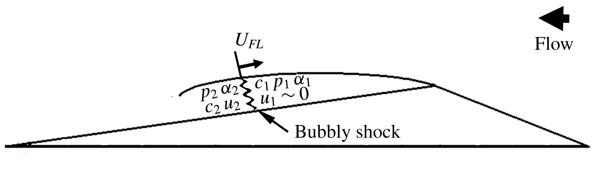
Diagram of a nominally one-dimensional bubbly shock propagating within the cavity.

5.1 Propagation of a one-dimensional shock in the bubbly mixture
We will use conservation of mass and momentum across a one-dimensional stationary shock to estimate the shock speed. The schematic of a the shock front is shown in figure 27. Across the shock front, we have
 $$\begin{eqnarray}\displaystyle & \displaystyle \unicode[STIX]{x1D70C}_{1}U_{1}=\unicode[STIX]{x1D70C}_{2}U_{2}, & \displaystyle\end{eqnarray}$$
 $$\begin{eqnarray}\displaystyle & \displaystyle p_{1}+\unicode[STIX]{x1D70C}_{1}{U_{1}}^{2}=p_{2}+\unicode[STIX]{x1D70C}_{2}{U_{2}}^{2}, & \displaystyle\end{eqnarray}$$
 $$\begin{eqnarray}\displaystyle & \displaystyle \unicode[STIX]{x1D70C}_{i}\approx \unicode[STIX]{x1D70C}_{L}(1-\unicode[STIX]{x1D6FC}_{i}). & \displaystyle\end{eqnarray}$$
 $$\begin{eqnarray}\displaystyle {U_{1}}^{2}=\frac{(p_{2}-p_{1})}{\unicode[STIX]{x1D70C}_{L}}\left[\frac{(1-\unicode[STIX]{x1D6FC}_{2})}{(1-\unicode[STIX]{x1D6FC}_{1})(\unicode[STIX]{x1D6FC}_{1}-\unicode[STIX]{x1D6FC}_{2})}\right]. & & \displaystyle\end{eqnarray}$$
Equation (5.4) does not take account of energy conservation across the shock, and the influence of bubble dynamics and surface tension are neglected. The speed expressed in
 $U_{1}$
is equal to the shock propagation speed into a stationary bubbly mixture.
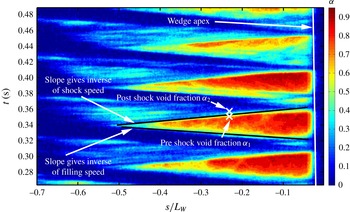
Measurement of front propagation speed from a space–time diagram of the cavity void fraction,
 $\unicode[STIX]{x1D6FC}$
, based on X-ray densitometry measurements. The void fraction is measured on a line parallel to the wedge in the
 $s$
direction at a constant distance
 $n=4$
mm from the wedge surface. The growth of the cavity and the propagation of the void-fraction shock are shown.

5.2 Measured speed of the propagating front
From time-resolved void-fraction flow field measurements, the velocity of the propagating front in the laboratory frame can be determined. For an observer stationary in the laboratory frame of reference, the front travels in a direction opposite to the mean flow direction outside the cavity. Thus the time evolution of the void-fraction fields can be used to estimate the front propagation speed if we assume that the propagation speed of the cavity contents upstream of the front is negligible. Figure 27 illustrates the front speed in the laboratory frame,
 $U_{FL}$
. By plotting the variation of void fraction as a function of time along the
 $s$
direction (figure 2) at a constant distance
 $n/L_{W}=0.02$
from the wedge surface, the velocity of the front,
 $U_{FL}$
, can be determined, as shown in figure 28. An isocontour line represented by an increasing slope in the
 $s$
–
 $t$
plane represents the cavity collapse speed. Similarly the cavity growth rate can be estimated by calculating the slope of the line with a decreasing slope in the
 $s$
–
 $t$
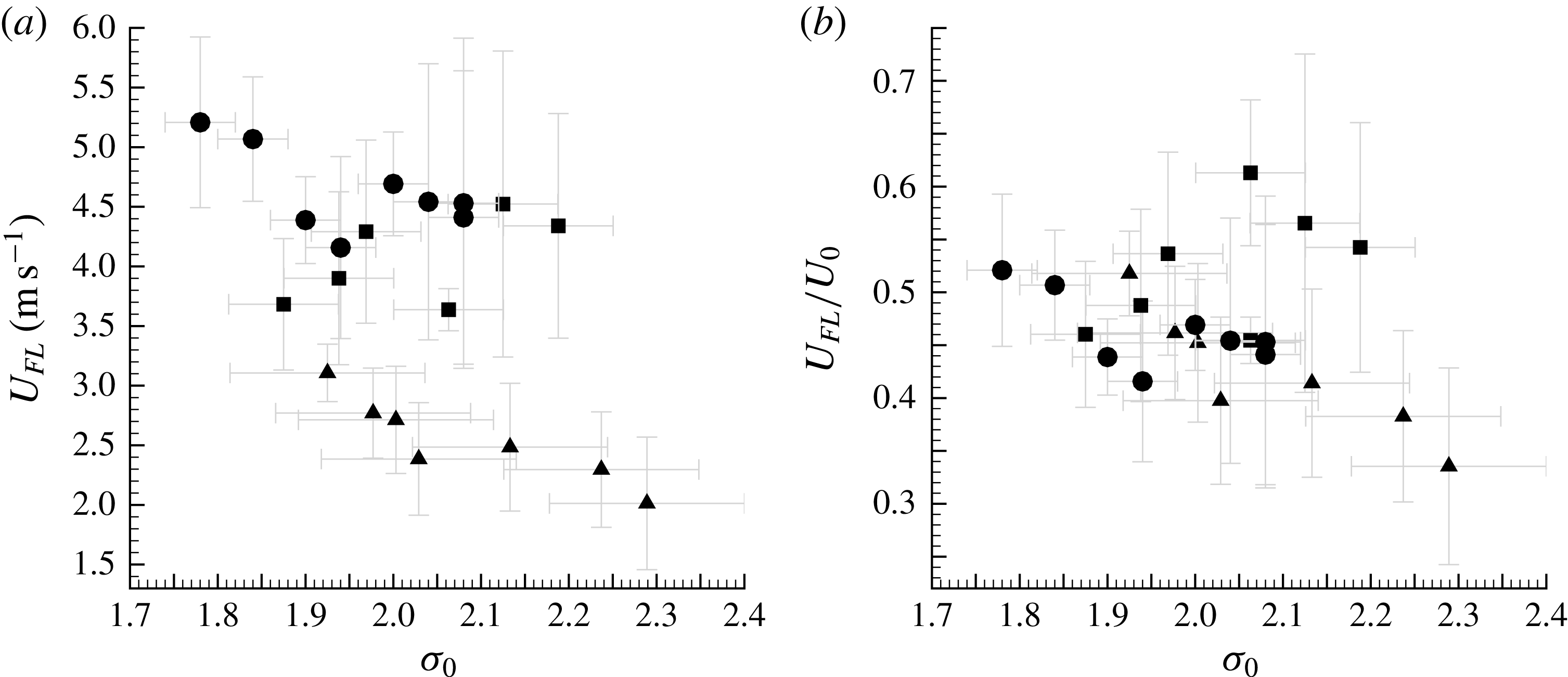
plane. The speeds thus determined depend upon the cavitation number for a given inlet speed. Figure 29(a) shows the front speed
 $U_{FL}$
for different inlet speeds and cavitation numbers, and figure 29(b) shows the variation of ratio of
 $U_{FL}/U_{0}$
. With an increase in speed, the front speed in the laboratory frame increased. The variation in the front speed is mainly due to the variability between different cycles, not the uncertainty of the measurement itself.
(a) The propagation speed of the void-fraction front measured in the laboratory frame,
 $U_{FL}$
, versus cavitation number,
 $\unicode[STIX]{x1D70E}_{0}$
, for three free-stream speeds
 $U_{0}=6~\text{m}~\text{s}^{-1}$
(▴), 8 m s
 $^{-1}$
(▪) and 10 m s
 $^{-1}$
(●); (b) the data plotted as the ratio
 $U_{FL}/U_{0}$
.

5.3 Void fraction across the propagating front
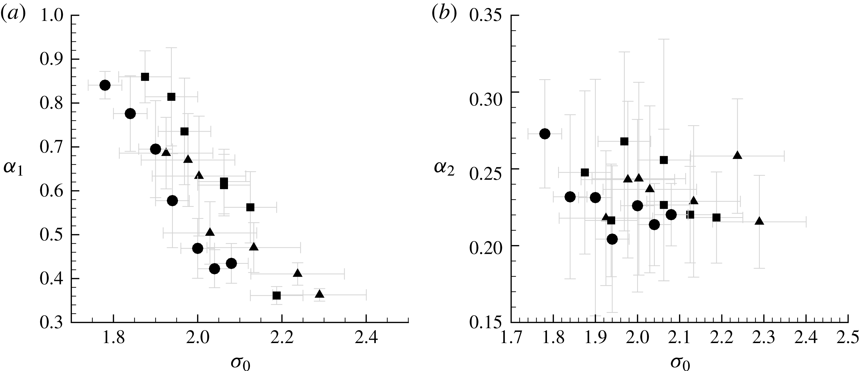
Figure 30(a,b) shows the variation of pre- and post-front void fraction,
 $\unicode[STIX]{x1D6FC}_{1}$
and
 $\unicode[STIX]{x1D6FC}_{2}$
, for varying cavitation numbers. The pre- and post- front void-fraction values were averaged for a number of cycles, and the pre-front void fraction increased with a decrease in cavitation number for all speeds. The inlet speed has a weak effect on the void fraction after the passage for the front, with
 $\unicode[STIX]{x1D6FC}_{2}\approx 0.22$
for all speeds. The nominal thickness of the front is approximately 3 mm, which is significantly higher than the spatial resolution X-ray system which was 0.5 mm (Mäkiharju Reference Mäkiharju2012), albeit non-parallel beam paths. Another factor that can contribute to thicker observed shock fronts in X-ray measurements is non-two-dimensional nature (spanwise variations) of the propagating shock front. Also, a propagating bubbly shock would not have a sharp front but would have finite thickness related to the dynamics of the collapsing cavitation bubbles, as discussed by Brennen (Reference Brennen2005). The length scale of the bubbles within the high void-fraction cavitating portion of the cavity, prior to the passage of the front, is expected to be of the order of 100 microns and the shape to be highly non-spherical, as shown by Coutier-Delgosha et al. (Reference Coutier-Delgosha, Devillers, Pichon, Vabre, Woo and Legoupil2006). Therefore, we can expect the thickness of the front to be a multiple of this length scale.
The void fraction upstream of the front,
 $\unicode[STIX]{x1D6FC}_{1}$
, and downstream of the front,
 $\unicode[STIX]{x1D6FC}_{2}$
, versus cavitation number,
 $\unicode[STIX]{x1D70E}_{0}$
, for three free-stream speeds
 $U_{0}=6~\text{m}~\text{s}^{-1}$
(▴), 8 m s
 $^{-1}$
(▪) and 10 m s
 $^{-1}$
(●).

5.4 Pressure rise across the propagating front
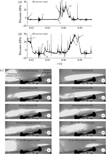
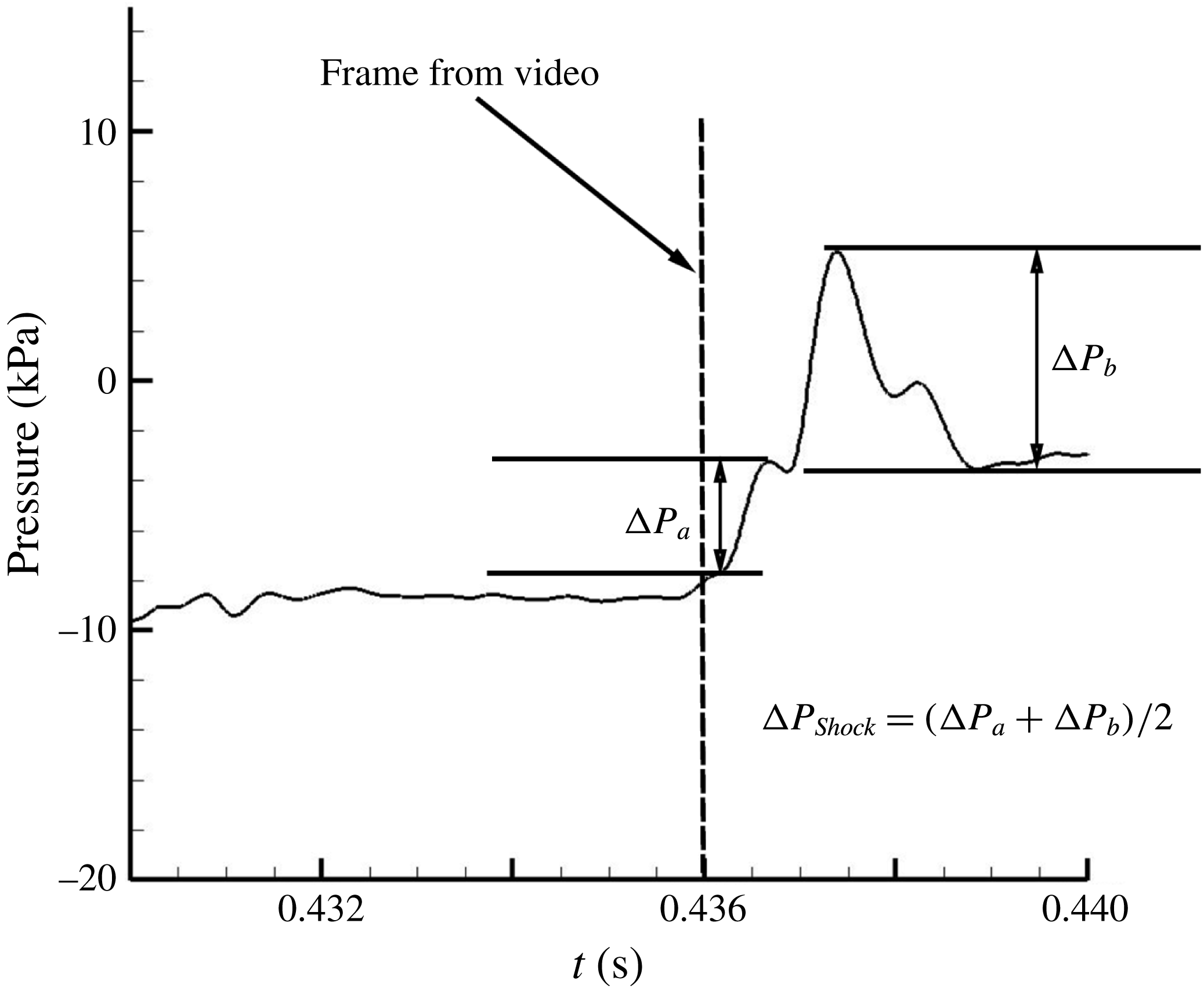
Examining equation (5.4), the difference between pressures should increase for increasing shock speeds, provided the void-fraction flow field remains unchanged and the observed change in void fraction across the front does not change drastically with the inlet speed for a given cavitation number. However, the front speed increased with an increase in inlet speed. Thus, we expect that the pressure rise across the front should increase with increase in inlet speed, if the front is behaving similar to a shock. Using time synchronous measurements of the time-expanded dynamic pressure signal, we can measure pressure difference on the surface of the wedge as the front passes over the transducer. A time series showing the unprocessed X-ray images and the corresponding pressure signals are shown in figure 31(a,b). The events corresponding to different points on the unsteady pressure signals are shown in figure 31(a,b), designated as roman numerals (i–x). The corresponding flow events are shown in figure 31(c). It can be seen that the passage of the shock over the transducer can be clearly identified for certain cycles. Based on the instant of time in the video when the shock crosses the transducer, the pressure signal can be probed to identified the pressure rise due to the passage of the shock.
Figure 32 is an image of the pressure trace obtained as the front moves across the face of the transducer after applying a digital filter. It is important to remember that the X-ray images of the front represent spanwise-averaged void-fraction measurements, while the face of the transducer is located along the centreline of the wedge and experiences only a portion of the front. Also, the face of the transducer is a circle with 6 mm diameter, which is wide when compared to the thickness of the front. Thus, the pressure signature of the passing front is often less well defined and repeatable compared to the images obtained from the X-ray system. Even under these difficult conditions, however, we are able to discern the pressure rise associated with the passage of the front. The pressure rise increased with inlet speeds (higher front propagation speeds), for a given cavitation number.
Example time traces of the dynamic pressure measured as the shock passes over the transducers
 $T_{1}$
and
 $T_{2}$
for a periodically shedding cavity are shown in (a,b). Simultaneously acquired X-ray shadowgraph images of the cavity are also shown in (c).

A time-expanded view of the pressure signal as the front passes over the face of the dynamic pressure transducer.

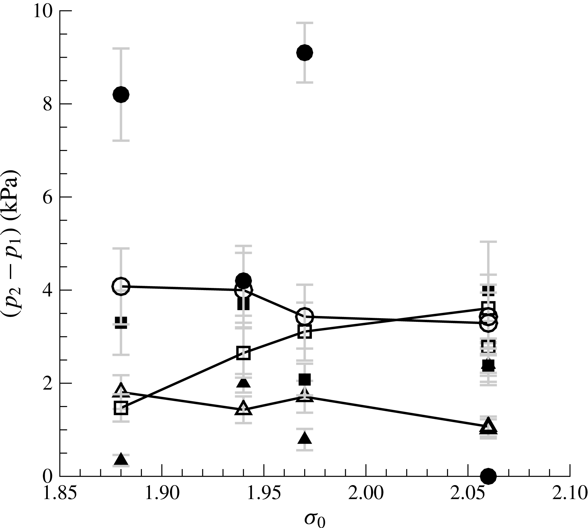
Comparison of predicted and measured pressure rise, (
 $p_{2}-p_{1}$
), across the shock for varying cavitation number,
 $\unicode[STIX]{x1D70E}_{0}$
, for three inlet speeds
 $U_{0}=6~\text{m}~\text{s}^{-1}$
(▴), 8 m s
 $^{-1}$
(▪) and 10 m s
 $^{-1}$
(●). Solid symbols represent measured pressure difference and the open symbols connected by a solid line represent the calculated value based on equation (5.4).

5.5 The predicted and measured pressure rise across the shock
In addition to measurements from pressure signals, we can use (5.4) to estimate the pressure rise (
 $p_{2}-p_{1}$
) across a bubbly shock based on the observed values of the front speed
 $U_{FS}$
and pre-and post-shock void fractions
 $\unicode[STIX]{x1D6FC}_{1}$
and
 $\unicode[STIX]{x1D6FC}_{2}$
. We will assume the
 $U_{FS}$
is equivalent to
 $U_{1}$
, which implies that the front is propagating into negligibly low-speed flow. The computed values for shock propagation are then compared to the measured pressure rise across the moving front. Figure 33 shows the measured pressure rise across the front as a function of cavitation number and for the three inlet speeds. The order of magnitude of the pressure rise is only a few kilopascals, making the rise of the order of the water vapour pressure itself. The magnitude of the measured pressure rise increases with increasing speed. This is also consistent with the mean cavity pressure data presented in § 4.6, where the absolute cavity pressure downstream of the cavity separation also increased in magnitude with an increase in inlet speed
 $U_{0}$
, and the magnitude of the pressure was of the order of 1 to 10 kPa.
Two trends in the data are observed. First, the predicted and measured pressure rises are of the same order. And second, there is a trend of increasing pressure rise with increasing speed. At the lower cavitation numbers, the predicted pressure rise is less than the measured speed by up to a factor of two. These data confirm that the jump conditions expressed in equation 5.4 are consistent with the observed propagation of the void-fraction fronts and thus strongly support the observation that a bubbly shock is present within the cavity.
6 Shock formation and the cavity Mach number
We have shown how, with a reduction in cavitation number, a transitional cavity that exhibits re-entrant cavity shedding can begin to intermittently develop bubbly shock fronts. With a further modest reduction in inlet pressure of just a few kilopascals, the cavity dynamics will become dominated by a cycle of cavity growth, shock formation and propagation and vapour cloud pinch off at the cavity separation (wedge apex). We will now examine how the reduction in sound speed of the bubbly mixture within the cavity is related to the sustained formation of shocks and, thus, the transition from a transitionally stable cavity to one that exhibits a strong cyclic shedding of cloud cavitation.
6.1 The speed of sound in the bubbly mixture upstream of the shock
High void fractions within the partial cavities leads to reduced sound speeds of the bubbly mixture that can fall below that of the inlet flow speed. Shamsborhan et al. (Reference Shamsborhan, Coutier-Delgosha, Caignaert and Nour2010) confirmed that the sound speed of a cavitating bubbly flow at an ambient pressure
 $p$
can be approximated by the relationship of Brennen (Reference Brennen2005) for a two-component mixture:
 $$\begin{eqnarray}\displaystyle \frac{1}{c^{2}}=[\unicode[STIX]{x1D70C}_{L}(1-\unicode[STIX]{x1D6FC})+\unicode[STIX]{x1D70C}_{G}\unicode[STIX]{x1D6FC}]\left[\frac{\unicode[STIX]{x1D6FC}}{k(p-p_{v})}+\frac{(1-\unicode[STIX]{x1D6FC})}{\unicode[STIX]{x1D70C}_{L}{c_{L}}^{2}}\right]. & & \displaystyle\end{eqnarray}$$
The subscript
 $G$
denotes the vapour phase of the bubbly mixture and
 $L$
denotes the liquid phase. Here we neglect surface tension and bubble dynamics and we assume the gas is polytropic;
 $c_{L}$
is the speed of sound of the pure water,
 $c_{L}=1480~\text{m}~\text{s}^{-1}$
and
 $k=1.3$
is the polytropic index of the water vapour. The density of the water vapour is
 $\unicode[STIX]{x1D70C}_{G}=0.02~\text{kg}~\text{m}^{-3}$
and the density of the water is
 $\unicode[STIX]{x1D70C}_{L}=1000~\text{kg}~\text{m}^{-3}$
. The sound speed of the bubbly mixture within the cavity is strongly related to both the void fraction and the difference of the mixture pressure from the liquid vapour pressure. For the flow conditions in the present study, the speed of sound of the bubbly mixture can fall to just a few metres per second. In the case of isothermal sound propagation, (
 $k=1$
) the calculated speed of sound is reduced by
 $0.5~\text{m}~\text{s}^{-1}$
from the polytropic value, which is within the measurement uncertainty.
The sound speed of the bubbly mixture upstream of the shock,
 $C_{1S}$
, versus cavitation number,
 $\unicode[STIX]{x1D70E}_{0}$
, for three inlet speeds
 $U_{0}=6~\text{m}~\text{s}^{-1}$
(▴), 8 m s
 $^{-1}$
(▪) and 10 m s
 $^{-1}$
(●).

The void fraction of the mixture upstream of the shock is shown in figure 30(a) and the mean pressure of the bubbly flow is shown in figure 26(b). Therefore, we can use equation (6.1) to determine the sound speed of the bubbly flow upstream of the observed shocks, which we will denote as
 $C_{1S}$
; and we will define a Mach number based on the average flow velocity across the cavity throat,
 $M_{1}^{\ast }$
:
 $$\begin{eqnarray}\displaystyle {M_{1}}^{\ast }=\left[\frac{U_{0}}{(1-\unicode[STIX]{x1D706})}\frac{1}{C_{1S}}\right]. & & \displaystyle\end{eqnarray}$$
We can also define a Mach number based on the observed shock propagation speed in the laboratory frame,
 $M_{FL}^{\ast }$
:
 $$\begin{eqnarray}\displaystyle M_{FL}^{\ast }=\frac{U_{FL}}{C_{1S}}. & & \displaystyle\end{eqnarray}$$
Figures 34–36 present the
 $C_{1S}$
,
 $M_{1}^{\ast }$
and
 $M_{FL}^{\ast }$
for three inlet speeds. The speed of sound in the mixture upstream of the shock front ranges from
 $1~\text{m}~\text{s}^{-1}<C_{1S}<10~\text{m}~\text{s}^{-1}$
, which is substantially slower than the average speed of the liquid flow through the throat of 9 to 15 m s
 $^{-1}$
. The speed of sound is slightly higher for higher inlet speeds. However, the Mach number
 $M_{1}^{\ast }$
is does not have a dependence on inlet speed. This is shown in the plot of
 $M_{1}^{\ast }$
, where the Mach number is consistently above unity. However, the Mach number based on the observed speed of the shock front does not reach unity except for the strongly shedding cases corresponding to periodic shedding, when
 $\unicode[STIX]{x1D70E}_{0}<1.9$
.
Mach number based on average throat speed,
 $M_{1}^{\ast }$
, versus cavitation number,
 $\unicode[STIX]{x1D70E}_{0}$
, for three free-stream speeds
 $U_{0}=6~\text{m}~\text{s}^{-1}$
(▴), 8 m s
 $^{-1}$
(▪) and 10 m s
 $^{-1}$
(●).

Mach number based on measured shock speed,
 $M_{FL}$
, versus cavitation number,
 $\unicode[STIX]{x1D70E}_{0}$
, for three free-stream speeds
 $U_{0}=6~\text{m}~\text{s}^{-1}$
(▴), 8 m s
 $^{-1}$
(▪) and 10 m s
 $^{-1}$
(●).

Time traces of
 $\unicode[STIX]{x1D6FC}_{1}(t)$
,
 $C_{1}(t)$
and
 $M_{1}(t)$
, for the transitory cavity,
 $\unicode[STIX]{x1D70E}_{0}=2.13$
. The dashed in (b) line represents the sound speed for shock formation,
 $C_{1S}$
, and the dashed line in (c) represents the threshold Mach number values for shock formation,
 $M_{1}^{\ast }$
.

Time traces of
 $\unicode[STIX]{x1D6FC}_{1}(t)$
,
 $C_{1}(t)$
, and
 $M_{1}(t)$
, for the periodically shedding cavity,
 $\unicode[STIX]{x1D70E}_{0}=1.95$
. The dashed in (b) line represents the sound speed for shock formation,
 $c_{1S}$
, and the dashed line in (c) represents the threshold Mach Number values for shock formation,
 $M_{1}^{\ast }$
.

6.2 The time-varying sound speed of the transitional and shedding cavities
It is important to note that the shock properties identified above are for local flow conditions that were observed around a shock that was present for any given cavitation number. However, the probability that a shock would form was much lower for incipient and transitional cavities, where shock formation was intermittent. Thus, it is instructive to compare the time-varying Mach number within the cavity to the Mach number observed during the occurrence of a strong shock front. We will define the local, time-varying Mach number as
 $$\begin{eqnarray}\displaystyle M_{1}(t)=\left[\frac{U_{0}}{(1-\unicode[STIX]{x1D706})}\frac{1}{C_{1}(t)}\right], & & \displaystyle\end{eqnarray}$$
where
 $C_{1}(t)$
is a function of the mean cavity pressure,
 $p_{D}$
, and the time-varying void fraction
 $\unicode[STIX]{x1D6FC}_{1}(t)$
measured upstream of the shock. The local void fraction was measured in the cavity region shown in figure 2(b) which was consistently upstream of the strong shocks. A control volume of 5 by 8 mm in the
 $s$
and
 $n$
direction around the point VF was chosen for spatially averaging void-fraction values. Figures 37 and 38(a–c) present time-series data for a transitionally shedding cavity and for a periodically shedding cavity. The time varying
 $\unicode[STIX]{x1D6FC}_{1}(t)$
,
 $C_{1}(t)$
and
 $M_{1}(t)$
are shown. Also shown are the values of
 $C_{1S}$
and
 $M_{1}^{\ast }$
corresponding the speed of sound and the Mach number observed for strong shocks at the particular cavitation number,
 $\unicode[STIX]{x1D70E}_{0}$
. Figure 37 shows data for
 $\unicode[STIX]{x1D70E}_{0}=2.13$
, a condition where shocks were rarely observed, and it is clear that the time-varying void fraction is not high enough on average to produce a local Mach number sufficient to sustain the formation of shocks. However, when the cavitation number is reduced to
 $\unicode[STIX]{x1D70E}_{0}=1.95$
, as shown figure 38, the local Mach consistently exceeds the critical value.
Distribution of the Mach number ratio
 $M_{1}/M_{1}^{\ast }$
presented with box plots for varying cavitation number,
 $\unicode[STIX]{x1D70E}_{0}$
, at three inlet speeds
 $U_{0}=6~\text{m}~\text{s}^{-1}$
(a), 8 m s
 $^{-1}$
(b) and 10 m s
 $^{-1}$
(c). The boxes present the median and the first and third quartiles of the Mach number distribution. The upper whisker on the box represents the 75th percentile plus 1.5 times the difference between the 75th and 50th percentile. The lower whisker on the box represents the 25th percentile minus 1.5 times the difference between the 50th and 25th percentiles. Dashed dotted line represents
 $M_{1}/M_{1}^{\ast }=1$
.

The likelihood that the local Mach number within the cavity will reach the critical value is illustrated in figures 37 and 38. In figure 39 we present a box plot of the ratio
 $M_{1}(t)/M_{1}^{\ast }$
for varying
 $\unicode[STIX]{x1D70E}_{0}$
. When the ratio reaches a value of unity, the critical Mach number for shock formation is reached. At higher cavitation numbers, both the mean and standard deviation of the Mach number ratio fall below unity, making the formation of a shock possible, but unlikely. With decreasing cavitation number, the likelihood that the ratio exceeds unity increases, along with the chances for the formation of a shock, even though the average value of the Mach number still falls below the critical value. Finally, with a sufficient reduction in sound speed, the average value of
 $M_{1}(t)/M_{1}^{\ast }$
exceeds unity, making shock formation extremely likely. Hence, we have passed from a transitional to strongly shedding condition. This behaviour is observed at all speeds, despite different shock speeds and shedding frequencies.
7 Discussion and conclusions
Cavitation dynamics in the separated region of flow at a wedge apex was studied by systematically changing the inlet cavitation number. The cavity remained stable exhibiting a bubbly frothy wake for
 $\unicode[STIX]{x1D70E}_{0}>2.1$
, exhibited tendencies of shedding
 $1.9<\unicode[STIX]{x1D70E}_{0}<2.1$
and well-defined periodic shedding for
 $\unicode[STIX]{x1D70E}_{0}<1.9$
. The observed trends of cavity length and thickness variation were found to be consistent with analytically predicted values using free-streamline theory. For stable cavities, the cavity shape matched the analytically predicted shape until the point of maximum thickness, as previously observed in other studies.
The dynamics of a time-varying cavity was also analysed using surface pressure signals and void-fraction measurements using X-ray densitometry. The calculated values of Strouhal number suggest that the present dynamics is similar to that reported in the literature. Further analysis of time-averaged void-fraction flow fields revealed a weak dependence of the averaged void-fraction profiles on the inlet speed. Time-resolved void-fraction flow fields of unsteady cavities revealed the presence of two different types of mechanisms associated with shedding cavities. The first is the classical liquid re-entrant jet-induced shedding, which causes shedding of vapour clouds. A second mechanism related to bubbly shock propagation was the principal reason for the strong, periodic cloud-shedding. With the help of the void-fraction flow field measurements and the static pressure at the wedge apex and the underneath the cavity, it was found that the observed shock waves broadly satisfied simple one-dimensional jump relations across the shocks.
Conditions necessary for the existence of shocks that caused shedding were found by comparing the local speed of sound values. The transition to strongly shedding conditions was associated with a drop in the sound speed of the bubbly mixture within the partial cavity, and the strongest shock waves occurred for Mach numbers in excess of unity. The dynamics of the shock wave is related to the local void fraction in the cavity, the small difference between the cavity static pressure and vapour pressure and the rate of pressure recovery in the cavity closure region. For the cavity examined in the present study, the collapse of the shed cavity did not appear to strongly affect the growth of the cavity as it starts a new shedding cycle. However, this may not necessarily be the case for all partial cavity shedding cycles.
Observance of the influence of the inlet velocity on the observed cavity dynamics shows that broad features of the cavity, such as cavity length, Strouhal number and apex pressure coefficient, do not change with changes in inlet speed. The average void-fraction distribution does not seem to strongly depend on the inlet velocity as well. Increased cavity pressure also result in increased shock speeds which manifest with an in increase in shedding frequency with increase in speed.
It is interesting to note that both the analytical model and basic jump relations related to one-dimensional bubbly shock propagation seemingly capture the most basic elements of the cavity shape and dynamics. The free-streamline model predicts the basic shape of the separated cavity region, even when the cavity consists of a bubbly mixture instead of pure vapour, and this suggests that the assumption that the cavity is at a nearly constant pressure is adequate, at least upstream of the position of maximum cavity thickness. The shock propagation and sound mixture sound speed models also appear to adequately capture the shock dynamics. These models do not consider the bubble dynamics within the cavity flow, including the complex topology of the gas phase at high cavity void fractions, as discussed by Coutier-Delgosha et al. (Reference Coutier-Delgosha, Devillers, Pichon, Vabre, Woo and Legoupil2006), nor is the constant production of vapour at the cavity detachment included in the modelling.
The propagation of bubbly shock waves can be an important, if not dominant, mechanism for the transition from stable sheet to cloud cavitation for cavities that consist of bubbly mixtures, rather than a pocket of gas or vapour alone. And, just as the model geometry can lead to three-dimensional re-entrant flows, shock propagation within the cavity need not be one-dimensional.
Acknowledgements
This work was funded by Office of Naval Research, grant no. N00014-14-1-0292, under program manager Dr K.-H. Kim. The authors would also like to acknowledge Mr A. Mallegol and Mr C. L. Jeune of the French naval academy for their contribution in the analytical study, and Mr T. Sun, visiting student from Harbin Institute of Technology, for his assistance in data processing.
Supplementary movies
Supplementary movies are available at http://dx.doi.org/10.1017/jfm.2016.425.