






1 Introduction
1.1 Motivation and Background
We recall that a linear recurrence sequence
 $\left (u_n\right )_{n=1}^{\infty }$
of order k over a field
 ${\mathbb K}$
is a sequence which satisfies a relation of the form
 $$ \begin{align} u_{n+k} = A_{k-1} u_{n+k-1} + \cdots + A_0 u_n, \qquad n\geqslant 0, \end{align} $$
with some constants
 $A_0, \ldots , A_{k-1}, u_0,\ldots ,u_{k-1}\in {\mathbb K}$
; we refer to [Reference Everest, van der Poorten, Shparlinski and Ward18] for a background on recurrence sequences.
It is well known by the celebrated Skolem–Mahler–Lech theorem, see for example [Reference Everest, van der Poorten, Shparlinski and Ward18, Theorem 2.1], that the set of zeros of a linear recurrence sequence
 $(u_n)_{n=0}^{\infty }$
, that is, the set of
 $n\in {\mathbb N}$
such that
 $u_n=0$
, is the union of a finite set with finitely many arithmetic progressions. The famous Skolem problem is a problem of decidability of the existence of such a zero. This problem remains widely open for most of the interesting fields
 ${\mathbb K}$
of characteristic zero, including
 ${\mathbb K}= {\mathbb Q}$
for
 $k\geqslant 5$
, a brief outline of the current state of affairs is given by Sha [Reference Sha33]. In particular, although there are very good, uniform in all parameters and depending only on k, bounds on the number of zeros, see [Reference Amoroso and Viada3], there are no effectively computable bounds on the index n of a possible zero
 $u_n = 0$
.
Here, we address a parametric version of this problem for a family of linear recurrence sequences and for all but finitely many values of the parameter for which the specialized sequence is not degenerate we give a bound on the largest possible zero. In particular, the Skolem problem is effectively decidable for all but a set of values of bounded height of the parameter
 $\alpha \in \overline {\mathbb Q}$
.
More precisely, we now recall that if the characteristic polynomial
 $$ \begin{align*} \Psi(Z) = Z^k - A_{k-1} Z^{k-1} - \cdots - A_0 \end{align*} $$
has k distinct roots
 $\lambda _1, \ldots , \lambda _k$
then for any sequence
 $(u_n)_{n=1}^{\infty }$
as in (1.1) there are some
 $\mu _1, \ldots , \mu _k$
in an algebraic extension of
 ${\mathbb K}$
such that
 $$ \begin{align*} u_n = \sum_{i=1}^k \mu_i \lambda_i^n, \qquad n \geqslant 0. \end{align*} $$
Linear recurrence sequences of this type are called simple. Some of the results on zeros of linear recurrence sequences in our arguments, are also known for arbitrary sequences, for example, those of [Reference Sha33], but some are known only under this condition, for example, those of [Reference Amoroso, Masser and Zannier2].
In the case of
 ${\mathbb K} = {\mathbb C}$
, the characteristic roots
 $\lambda _i$
,
 $i =1, \ldots , k$
, of the largest absolute value, that is, with
 $$ \begin{align*} |\lambda_i| = \max\{|\lambda_1|, \ldots, |\lambda_k|\} \end{align*} $$
are called dominant and play a major role in investigating various Diophantine properties of linear recurrence sequences.
We recall that a sequence
 $(u_n)_{n=1}^{\infty }$
satisfying (1.1) is called degenerate if one of the ratios
 $\lambda _i/\lambda _j$
,
 $1 \leqslant i < j < k$
, is a root of unity. We call a sequence nondegenerate otherwise.
It is very well-known that the Skolem problem for a degenerate sequence
 $u_n$
can be reduced to a series of the Skolem problems for finitely many nondegenerate sequences of the form
 $u_{nh+j}$
,
 $ j=0, \ldots , h-1$
, where h is bounded only in terms of the degree
 $[{\mathbb Q}(\lambda _1, \ldots , \lambda _k): {\mathbb Q}]$
, see [Reference Berstel and Mignotte5]. Hence, we are mostly interested in nondegenerate sequences.
Here, we study the case when both the coefficients
 $\mu _i$
and the roots
 $\lambda _i$
are rational functions of a parameter
 $\alpha \in \overline {{\mathbb Q}}$
. This scenario is close to that of Amoroso et al. [Reference Amoroso, Masser and Zannier2], see also [Reference Kulkarni, Mavraki and Nguyen24, Proposition 2.2]. In particular, we also appeal to some of the results from [Reference Amoroso, Masser and Zannier2], however, our method is based on a different argument.
More precisely, given two vectors of rational functions
 $$ \begin{align*} \mathbf{a}= \left(a_1,\ldots,a_k\right), \, \mathbf{f} = \left(f_1,\ldots,f_k\right)\in\overline{\mathbb Q}(X)^k, \end{align*} $$
over the algebraic closure
 $\overline {\mathbb Q}$
of
 ${\mathbb Q}$
we consider linear recurrence sequences of the form
 $$ \begin{align} F_n(X) = \sum_{i=1}^k a_i f_i^n, \qquad n \geqslant 0. \end{align} $$
We give a bound for the largest zero in (all but finitely many) specializations of this sequence such that the new sequence is not degenerate, see Theorem 2.1. This is based on recent results of Pakovich and the second author [Reference Pakovich and Shparlinski32] about finiteness of points on curves that lie on the unit circle, a bound for the largest zero in a linear recurrence with at most two dominant roots due to Sha [Reference Sha33] and a result of Amoroso et al. [Reference Amoroso, Masser and Zannier2, Theorem 1.5] giving an upper bound for the height of zeros of polynomials of the form (1.2). We then couple our result with a general ABC theorem for polynomials [Reference Bombieri and Gubler8, Theorem 12.4.4] to give a lower bound on the degree of the splitting field of
 $F_n$
over
 ${\mathbb Q}$
when
 $a_i,f_i$
are all polynomials, see Corollary 2.5, which gives an explicit form of [Reference Amoroso, Masser and Zannier2, Example 2].
We also look at complex numbers which are zeros of two functions of the form (1.2), see Theorem 2.9. This is closely related to studying the greatest common divisors of elements of two sequences defined by such functions. This point of view has been introduced by Ailon and Rudnick [Reference Ailon and Rudnick1] for polynomials of the form
 $f^n-1$
and
 $g^m-1$
,
 $n,m \geqslant 1$
, and further developed in recent works [Reference Corvaja and Zannier16, Reference Levin26, Reference Levin and Wang27, Reference Ostafe31, Reference Pakovich and Shparlinski32] for different other sequences. In turn, this builds on number field analogues of this problem, initiated by Bugeaud et al. [Reference Bugeaud, Corvaja and Zannier14] for sequences of the form
 $a^n-1$
and
 $b^m-1$
,
 $n,m\geqslant 1$
, where
 $a,b\in {\mathbb Z}$
are multiplicatively independent, and further extended in many works, including generalisations to S-units [Reference Corvaja and Zannier15].
When we restrict to the set
 ${\mathbb U}$
of all roots of unity only, we can say more about the arithmetic structure of
 $F_n(\alpha )$
,
 $n\geqslant 1$
, as defined in (1.2), that is, for all but finitely many
 $\alpha \in {\mathbb U}$
we prove that the set of
 $n\in {\mathbb N}$
such that
 $F_n(\alpha )$
is a perfect mth power either contains an arithmetic progression, or it is finite, see Theorem 2.7. We conclude the paper with an independent result, Theorem 2.12, which says that a sequence of rational functions is a linear recurrence sequence if and only if for uncountably many
 $\alpha \in {\mathbb C}$
the specialisations of the sequence have the same property.
2 Main Results
2.1 Skolem Problem for Parametric Families
We use
 $M_{\mathbb K}$
to denote a complete set of inequivalent absolute values on a number field
 ${\mathbb K}$
, normalized so that the absolute Weil height
 $h:\overline {{\mathbb Q}}\to [0,\infty )$
is defined via v-adic valuations
 $\|\alpha \|_v$
as follows
 $$ \begin{align*}h(\alpha) = \sum_{v\in M_{\mathbb K}} \dfrac{[{\mathbb K}_v: \mathbb{Q}_v]}{[{\mathbb K}:\mathbb{Q}]}\log \max\left \{ \|\alpha\|_v, 1 \right\} , \end{align*} $$
where
 ${\mathbb K}$
is any number field containing
 $\alpha $
and
 ${\mathbb K}_v$
is the completion of
 ${\mathbb K}$
with respect to the absolute value v. See [Reference Bombieri and Gubler8, Reference Hindry and Silverman22, Reference Silverman36, Reference Zannier41] for further details on absolute values and height functions.
To formulate our results, we need to recall that a finite Blaschke product is a rational function
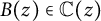 $B(z) \in {\mathbb C}(z)$
of the form
 $$ \begin{align} B(z)=\zeta\prod_{i=1}^n\left(\frac{z-a_i}{1-\bar{a_i}z}\right)^{m_i}, \end{align} $$
where
 $a_i$
are complex numbers in the open unit disc
 $\{z \in {\mathbb C}:|z| <1\}$
, the exponents
 $m_i$
,
 $i=1, \ldots , n$
, are positive integers, and
 $\left | \zeta \right |=1$
.
A rational function
 $Q(z)$
of the form
 $Q(z) = B_1(z)/B_2(z)$
, where
 $B_1$
and
 $B_2$
are finite Blaschke products, is called a quotient of finite Blaschke products.
We say that a pair of rational functions
 $\left (g_1(X), g_2(X)\right ) \in {\mathbb C}(X)^2$
is exceptional if they can be decomposed as
 $$ \begin{align} g_1=Q_1\circ g \qquad\text{ and}\qquad g_2=Q_2\circ g \end{align} $$
for some quotients of finite Blaschke products
 $Q_1$
and
 $Q_2$
and rational function g. Otherwise we say that
 $\left (g_1(X), g_2(X)\right )$
is a nonexceptional pair.
We recall that Blaschke products preserve the unit circle and thus come naturally in our investigation of
 $\alpha \in \overline {\mathbb Q}$
for which the corresponding specialisation of
 $F_n(X)$
given by (1.2) has at least three characteristic roots with the same modulus, that is, with
 $$ \begin{align*} |f_r(\alpha)|=|f_s(\alpha)|=|f_t(\alpha)|, \end{align*} $$
for some
 $1 \leqslant r< s < t \leqslant k$
, which implies
 $$ \begin{align*} \frac{|f_s(\alpha)|}{|f_r(\alpha)|}=\frac{|f_t(\alpha)|}{|f_r(\alpha)|}=1. \end{align*} $$
We see that if
 $g_1$
and
 $g_2$
are polynomials and thus have no finite poles, relations (2.2) are possible only if
 $n=1$
and
 $a_1 = 0$
in (2.1), in which case we obtain
 $$ \begin{align*}g_1= g^{m_1} \qquad\text{ and}\qquad g_2=g^{m_2}\end{align*} $$
for some
 $g\in {\mathbb C}[X]$
and integers
 $m_1, m_2 \geqslant 0$
.
Since as we have mentioned, the Skolem problem for degenerate sequences is easily reducible to the case of nondegenerate sequences, it motivates us to define for the parametric family (1.2) the exceptional set of
 $\alpha \in \overline {\mathbb Q}$
such that
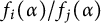 $f_i(\alpha )/f_j(\alpha )$
is not a root of unity for some
 $1 \leqslant i <j\leqslant k$
. It is also convenient to eliminate the roots of
 $a_i(X)$
and
 $f_i(X)$
,
 $1 \leqslant i \leqslant k$
. That is, we define the set
 $$ \begin{align*} {\mathfrak E}_{\mathbf{a},\mathbf{f}} = \{\alpha\in \overline{\mathbb Q}: f_i(\alpha)/f_j(\alpha)\text{ is a root of unity for some } 1 \leqslant i <j\leqslant k & \\ \text{or } a_i(\alpha)=0 \text{ or } f_i(\alpha) = 0 \text{ for some } 1 \leqslant i \leqslant k\}&. \end{align*} $$
Using [Reference Silverman36, Theorem 3.11], we immediately derive that elements of
 ${\mathfrak E}_{\mathbf {a},\mathbf {f}}$
are of bounded height.
Our first result is the following:
Theorem 2.1 Let
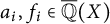 $a_i, f_i \in \overline {\mathbb Q}(X)$
,
 $i =1, \ldots , k$
, be nonzero rational functions of degree at most d such that
 $f_i/f_j$
is nonconstant for any
 $1 \leqslant i <j \leqslant k$
. We also assume that for any
 $1 \leqslant r<s <t \leqslant k$
, the pairs of rational functions
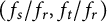 $(f_s/f_r, f_t/f_r)$
are nonexceptional. Let the sequence
 $(F_n)_{n=0}^{\infty }$
be defined by (1.2). Then for all but at most
 $2d^2 k(k-1)(k-2)/3$
elements
 $\alpha \in \overline {\mathbb Q} \setminus {\mathfrak E}_{\mathbf {a},\mathbf {f}}$
any zero
 $n\in {\mathbb N}$
of the equation
 $$ \begin{align} F_n(\alpha) = 0 \end{align} $$
satisfies
 $$ \begin{align*}n \leqslant \exp\left(C D^4_{\alpha}\right), \end{align*} $$
where
 $D_{\alpha }$
is the degree of the Galois closure of
 ${\mathbb Q}(\alpha )$
over
 ${\mathbb Q}$
and C is an effective constant which depends only on
 $a_1, f_1, \ldots , a_k, f_k$
.
Remark 2.2 We note that the condition that
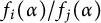 $f_i(\alpha )/f_j(\alpha )$
are not roots of unity for any
 $i\ne j$
is necessary for any bound on n as otherwise the sequence can have infinitely many zeros. However, if this is the case, then by the celebrated Skolem–Mahler–Lech theorem, see for example [Reference Everest, van der Poorten, Shparlinski and Ward18, Theorem 2.1], the set of zeros is the union of a finite set with finitely many arithmetic progressions, and by [Reference Berstel and Mignotte5] these arithmetic progressions can be effectively determined, while our method allows to estimate the elements in the remaining finite set.
It is natural to ask whether a generalization of Theorem 2.1 to parametric S-unit equations is possible, see Section 8 for more details and an exact question.
Theorem 2.1, immediately implies the following:
Corollary 2.3 Let
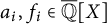 $a_i, f_i \in \overline {\mathbb Q}[X]$
,
 $i =1, \ldots , k$
, be as in Theorem 2.1
. Let
 ${\mathcal A}_D$
be the union of all Galois fields of degree at most D over
 ${\mathbb Q}$
. Then there is an effectively computable constant
 $C_0$
which depends only on
 $a_1, f_1, \ldots , a_k, f_k$
such that for all but at most
 $12 dD^2k^2 + 2d^2k^3/3$
elements
 $\alpha \in {\mathcal A}_D$
, any zero
 $n\in {\mathbb N}$
of the equation (2.3) satisfies
 $$ \begin{align*} n \leqslant \exp(C_0 D^4). \end{align*} $$
Combining Theorem 2.1 with a result of Amoroso et al. [Reference Amoroso, Masser and Zannier2, Theorem 1.5] (see Lemma 3.4), we also derive the following.
Corollary 2.4 Let
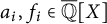 $a_i, f_i \in \overline {\mathbb Q}[X]$
,
 $i =1, \ldots , k$
, be as in Theorem 2.1. Then there exists a finite set
 ${\mathcal E}\subseteq \overline {\mathbb Q}$
such that for all roots
 $\alpha $
of
 $F_n$
,
 $n\geqslant 1$
, with
 $\alpha \not \in {\mathcal E} \cup {\mathfrak E}_{\mathbf {a},\mathbf {f}}$
the degree
 $D_{\alpha }$
of the smallest Galois extension over
 ${\mathbb Q}$
containing
 $\alpha $
satisfies
 $$ \begin{align*}D_{\alpha} \geqslant c (\log n)^{1/4}, \end{align*} $$
where c is an effective constant depending only on
 $a_1, f_1, \ldots , a_k, f_k$
.
Finally Theorem 2.1 coupled with a result of Fuchs and Pethö [Reference Fuchs and Pethö21, Corollary 3.1] (see Lemma 3.8) yields the following result.
Corollary 2.5 Let
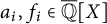 $a_i, f_i \in \overline {\mathbb Q}[X]$
,
 $i =1, \ldots , k$
, be as in Theorem 2.1
and such that
 $\gcd (a_1f_1, \ldots , a_kf_k)=1$
. Then the splitting field
 ${\mathbb L}_n$
of the polynomial
 $F_n$
defined by (1.2) is of degree
 $$ \begin{align*} [{\mathbb L}_n:{\mathbb Q}] \geqslant c_0 (\log n)^{1/4}, \end{align*} $$
where
 $c_0$
is an effective constant depending only on
 $a_1, f_1, \ldots , a_k, f_k$
.
Note that Corollary 2.5 provides an explicit version of the claim that
 $$ \begin{align*}[{\mathbb L}_n:{\mathbb Q}] \to \infty \end{align*} $$
as
 $n \to \infty $
given in [Reference Amoroso, Masser and Zannier2, Example 2].
The bound for n in Theorem 2.1 depends on the degree of the specialization
 $\alpha $
. We would like to obtain a bound which is independent of
 $\alpha $
, when we restrict
 $\alpha $
to special subsets of
 $\overline {\mathbb Q}$
, such as the set of all roots of unity. This in particular would imply that the set
 $$ \begin{align*} \{\alpha \in \overline{\mathbb Q} :\alpha^n=1,\ F_m(\alpha)=0 \text{ for some } n,m\geqslant 1\}, \end{align*} $$
is finite, where
 $F_m$
is defined by (1.2).
More generally, since
 $G_n(X)=X^n-1$
,
 $n\geqslant 1$
, also defines a linear recurrence sequence, we would like to generalise the above situation and formulate the following problem.
Question 2.6 Given two simple linear recurrence sequences
 $(F_n)_{n=1}^{\infty }$
,
 $(G_m)_{n=1}^{\infty }$
over
 ${\mathbb C}(X)$
, prove that, under certain conditions, the set
 $$ \begin{align} {\mathcal L}(F_n,G_m)=\{\alpha\in{\mathbb C} :F_n(\alpha)=G_m(\alpha)=0 \text{ for some } n,m\geqslant 1\} \end{align} $$
is finite.
This would extend the result of [Reference Amoroso, Masser and Zannier2] which already gives the boundedness of heights of
 $\alpha \in \overline {\mathbb Q}$
that satisfy only one such relation over
 $\overline {\mathbb Q}$
.
We answer Question 2.6 for binary sequences in Section 2.3, which is a direct consequence of [Reference Bombieri, Masser and Zannier10, Theorem 2]. We also prove a more general result which holds only over
 $\overline {\mathbb Q}$
, see Theorem 2.9.
2.2 Perfect Powers in Specializations at Roots of Unity
We now restrict
 $\alpha $
to the set
 ${\mathbb U}$
of all roots of unity. In this case, for all but finitely many
 $\alpha \in {\mathbb U}$
, we can effectively answer some other questions about
 $F_n(\alpha )$
besides vanishing. We illustrate this approach on the case of perfect powers.
We use
 ${\mathbb Z}_{\overline {\mathbb Q}}$
to denote the set of all algebraic integers in
 $\overline {\mathbb Q}$
.
We say that
 $\vartheta \in {\mathbb Z}_{\overline {\mathbb Q}}$
is a perfect mth power if for some
 $\rho \in {\mathbb Q}(\vartheta )$
, we have
 $\vartheta = \rho ^m$
.
For a polynomial
 $f\in {\mathbb C}[X]$
, we use
 $\overline {f}$
to denote the complex conjugate polynomial, that is, the polynomial obtained from f by conjugating all its coefficients.
Theorem 2.7 Let
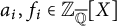 $a_i, f_i \in {\mathbb Z}_{\overline {\mathbb Q}} [X]$
,
 $i =1, \ldots , k$
, be nonzero polynomials of degree at most d such that for any
 $1 \leqslant r<s <t \leqslant k$
, the pairs of rational functions
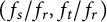 $(f_s/f_r, f_t/f_r)$
are nonexceptional. We also assume that for
 $1\leqslant i\ne j\leqslant k$
the polynomials
 $f_i(X)\overline {f_i}(Y) - f_j(X)\overline {f_j}(Y)$
do not have any factor of the form
 $X^rY^s-u$
or
 $X^r-uY^s$
where u is a root of unity. Let the sequence of polynomials
 $\left (F_n\right )_{n=0}^{\infty }$
be defined by (1.2). Then for all but at most
 $d^2(2k^3/3 + 22k^2)$
elements
 $\alpha \in {\mathbb U} \setminus {\mathfrak E}_{\mathbf {a},\mathbf {f}}$
for any
 $m \geqslant 1$
the set of
 $n\in {\mathbb N}$
such that
 $F_n(\alpha ) $
is a perfect mth power either contains an infinite arithmetic progression
 $m\ell +r$
,
 $\ell =1,2, \ldots, $
with some
 $r \in \{0, \ldots , m-1\}$
or is finite and its size can be effectively bounded.
Remark 2.8 We note that by a result of Lang [Reference Lang25] the set
 ${\mathbb U} \cap {\mathfrak E}_{\mathbf {a},\mathbf {f}}$
is in fact finite, thus the number of exceptions in Theorem 2.7 is finite.
2.3 Greatest Common Divisors of Binary Linear Recurrence Sequences
We note that the finiteness conclusion in Question 2.6 would imply that there are finitely many
 $\alpha \in \overline {\mathbb Q}$
such that
 $$ \begin{align*} (X-\alpha) \mid \gcd(F_n(X),G_m(X)) \end{align*} $$
for some
 $n,m\geqslant 1$
, where by the greatest common divisor of two rational functions, we mean the greatest common divisor of their numerators.
Studying the greatest common divisor of sequences of polynomials has been initiated in [Reference Ailon and Rudnick1] for sequences
 $F_n=f^n-1$
and
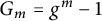 $G_m=g^m-1$
,
 $n,m\geqslant 1$
, where
 $f,g\in {\mathbb C}[X]$
, and recently extended in several directions in [Reference Corvaja and Zannier16, Reference Levin26, Reference Levin and Wang27, Reference Ostafe31, Reference Pakovich and Shparlinski32].
We note that in the case of simple binary linear recurrence sequences defined over
 ${\mathbb C}(X)$
, under a multiplicative independence condition, a finiteness result follows directly from [Reference Ostafe31, Theorem 1.3]. In fact, here, we consider a more general scenario, which however holds only when the rational functions involved are defined over
 $\overline {\mathbb Q}$
.
More precisely, for a finitely generated group
 $\Gamma \subseteq \overline {\mathbb Q}^*$
, we define the division group of
 $\Gamma $
to be the set
 $$ \begin{align*} \Gamma^{\mathrm{div}}=\{\alpha\in\overline{\mathbb Q} :\alpha^n \in \Gamma \text{ for some } n\geqslant 1\}. \end{align*} $$
Then, we have the following result.
We say that
 $\psi _1,\ldots ,\psi _t\in {\mathbb C}(X)$
are multiplicatively independent modulo a set
 ${\mathcal S} \subseteq {\mathbb C}$
if for all non-zero vectors
 $\left (h_1, \ldots , h_t\right ) \in {\mathbb Z}^t$
one has
 $$ \begin{align*}\psi_1(X)^{h_1} \ldots \psi_t(X)^{h_t} \not \in {\mathcal S}. \end{align*} $$
Theorem 2.9 Let
 $\Gamma \subseteq \overline {\mathbb Q}^*$
be a finitely generated subgroup. Let
 $f_1,\ldots ,f_r,g_1,\ldots ,g_s\in \overline {\mathbb Q}(X)$
be multiplicatively independent modulo
 $\Gamma $
. There exists a polynomial
 $h\in \overline {\mathbb Q}[X]$
depending only on
 $f_i,g_j$
and the generators of
 $\Gamma $
such that that for any nonzero vectors
 $(m_1,\ldots ,m_r)\in {\mathbb N}^r$
,
 $(n_1,\ldots ,n_s)\in {\mathbb N}^s$
and any
 $u,v \in \Gamma ^{\mathrm {div}}$
one has
 $$ \begin{align*}\gcd\left(\prod_{i=1}^rf_i(X)^{m_i}-u,\prod_{j=1}^sg_j(X)^{n_j}-v \right)\mid h. \end{align*} $$
Remark 2.10 Taking
 $r=s=2$
,
 $\Gamma =\{1\}$
,
 $m_1=n_1=1$
, and
 $u=v=-1$
in Theorem 2.9, one has the sequences
 $(F_n)_{n=1}^{\infty }$
,
 $(G_m)_{n=1}^{\infty }$
defined by
 $$ \begin{align*} &F_n(X)=f_1(X)f_2(X)^n+1, \quad n\geqslant 1,\\ &G_m(X)=g_1(X)g_2(X)^m+1, \quad m\geqslant 1. \end{align*} $$
In this case, the set
 ${\mathcal L}(F_n,G_m)$
, defined by (2.4), is finite and its cardinality is uniformly bounded only in terms of the functions
 $f_1,f_2,g_1,g_2$
. In fact, this conclusion holds also when
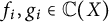 $f_i,g_i\in {\mathbb C}(X)$
,
 $i=1,2$
. Indeed, the proof follows directly from [Reference Ostafe31, Theorem 1.3], which is the same as the proof of Theorem 2.9 but instead of using Lemma 3.2 below, one uses [Reference Bombieri, Masser and Zannier11, Theorem] (which in turn generalises [Reference Bombieri, Masser and Zannier10, Theorem 2]). See also [Reference Bilu and Luca7] for some effective results for rational functions over
 ${\mathbb Q}$
and
 $G_m = X^m -1$
.
As a direct consequence of Theorem 2.9, we have the following result, which we hope to be of independent interest.
Corollary 2.11 Let
 $\Gamma \subseteq \overline {\mathbb Q}^*$
be a finitely generated subgroup. Let
 $f_1,\ldots ,f_r,g_1,\ldots ,g_s\in \overline {\mathbb Q}(X)$
be multiplicatively independent modulo
 $\Gamma $
. Then there exists a polynomial
 $H\in \overline {\mathbb Q}[X]$
such that for any nonzero vectors
 $(m_1,\ldots ,m_r)\in {\mathbb N}^r$
,
 $(n_1,\ldots ,n_s)\in {\mathbb N}^s$
and any polynomials
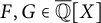 $F,G \in \overline {\mathbb Q}[X]$
of degree at most
 $d\geqslant 1$
with roots from
 $\Gamma ^{\mathrm {div}}$
, one has
 $$ \begin{align*}\gcd\left(F\left(\prod_{i=1}^rf_i(X)^{m_i}\right),G\left(\prod_{j=1}^sg_j(X)^{n_j}\right)\right) \mid H. \end{align*} $$
2.4 Specializations of Sequences of Rational Functions
Finally, we show that a sequence of rational functions
 $F_n(X) \in {\mathbb C}(X)$
,
 $n\geqslant 0$
, satisfies a linear recurrence relation if and only if this is also true for specialisations
 $F_n(\alpha )$
,
 $n\geqslant 0$
, for a sufficiently “massive” set of
 $\alpha \in {\mathbb C}$
.
Theorem 2.12 Let
 $\left (F_n\right )_{n=0}^{\infty }$
be an infinite sequence of rational functions
 $F_n\in {\mathbb C}(X)$
,
 $n\geqslant 0$
, and let
 $K\geqslant 1$
. Assume there exist infinitely many
 $\alpha \in {\mathbb C}$
such that each
 $F_n(\alpha )$
is well defined and
 $\left (F_n(\alpha )\right )_{n=0}^{\infty }$
is a linear recurrence of order at most K. Then
 $\left (F_n\right )_{n=0}^{\infty }$
is a linear recurrence sequence over
 ${\mathbb C}(X)$
of order at most K.
Theorem 2.12 implies that if
 $\left (F_n(\alpha )\right )_{n=0}^{\infty }$
is a linear recurrence sequence for uncountably many
 $\alpha \in {\mathbb C}$
(without any restriction on the order), then
 $\left (F_n\right )_{n=0}^{\infty }$
is a linear recurrence sequence in
 ${\mathbb C}[X]$
. Indeed, since the set of possible orders is countable, at least one order must occur for infinitely many
 $\alpha \in {\mathbb C}$
(in fact uncountably many
 $\alpha $
). On the other hand, just a condition of the infinitude of such
 $\alpha \in {\mathbb C}$
is not sufficient. For example, the sequence
 $$ \begin{align*}F_n(X) = X^{2^{n^2}+n} + X^{6^n} + X^{2^{{\left\lfloor{\sqrt{n}}\right\rfloor}}} + 3^n, \qquad n = 0,1, \ldots, \end{align*} $$
does not satisfy any linear recurrent relation (as the degree grows too fast). However, it is a linear recurrence sequence for specializations at any root of unity of order
 $2^m$
,
 $m =0, 1, \ldots .$
3 Preliminaries
3.1 Intersections of Level Curves of Rational Functions
Our approach depends on a generalisation of a result of Ailon and Rudnick [Reference Ailon and Rudnick1, Theorem 1] which is given in [Reference Pakovich and Shparlinski32, Theorem 2.2].
Recall the definition of nonexceptional pairs of rational functions, that is, pairs which do not satisfy relations of the form (2.2).
Lemma 3.1 Let
 $g_1(X), g_2(X) \in {\mathbb C}(X)$
be complex rational functions of degrees
 $n_1$
and
 $n_2$
, respectively. Then
 $$ \begin{align*}\# \{z \in {\mathbb C}:\left|g_1(z)\right | =\left| g_2(z)\right | =1\} \leqslant (n_1+n_2)^2, \end{align*} $$
unless
 $\left (g_1(X), g_2(X)\right )$
is exceptional.
As we have mentioned if
 $g_1$
and
 $g_2$
are polynomials then the conclusion of Lemma 3.1 holds except when
 $$ \begin{align*} g_1= g^{m_1} \qquad\text{and}\qquad g_2=g^{m_2} \end{align*} $$
for some
 $g\in {\mathbb C}[X]$
and integers
 $m_1, m_2 \geqslant 0$
.
3.2 Intersection of Parametric Curves with Division Groups
The proof of Theorem 2.9 is based on the following result which is a direct consequence of Maurin’s result [Reference Maurin30, Théorème 1.2]; see also [Reference Bombieri, Habegger, Masser and Zannier9] for an effective proof of [Reference Maurin30, Théorème 1.2].
Lemma 3.2 Let
 $\Gamma \subseteq \overline {\mathbb Q}^*$
be a finitely generated subgroup. Let
 $f_1, \ldots , f_n \in \overline {\mathbb Q}(X)$
be multiplicatively independent modulo
 $\Gamma $
. Then, there are only finitely many
 $\alpha \in \overline {\mathbb Q}$
such that there exist two linearly independent vectors
 $(k_1,\ldots ,k_n)$
,
 $(\ell _1,\ldots ,\ell _n)\in {\mathbb Z}^n$
such that
 $$ \begin{align*} f_1(\alpha)^{k_1}\cdots f_n(\alpha)^{k_n},\ f_1(\alpha)^{\ell_1}\cdots f_n(\alpha)^{\ell_n}\in \Gamma^{\mathrm{div}}. \end{align*} $$
Proof The proof follows directly from a result of Maurin [Reference Maurin30, Théorème 1.2] (see also [Reference Bombieri, Habegger, Masser and Zannier9, Theorem (Maurin)]). Indeed, let
 $\gamma _1,\ldots ,\gamma _r \in \Gamma $
be the generators of the group
 $\Gamma $
, and thus, they are multiplicatively independent elements. We define the parametric curve
 $$ \begin{align*} {\mathcal C}=\{(f_1(\alpha),\ldots,f_n(\alpha),\gamma_1,\ldots,\gamma_r) :\, \alpha \in \overline{\mathbb Q}\}\subset {\mathbb G}_{\mathrm{m}}^{n+r}. \end{align*} $$
For an element
 $\alpha \in \overline {{\mathbb Q}}$
, assume that there exist two linearly independent vectors
 $(k_1,\ldots ,k_n)$
,
 $(\ell _1,\ldots ,\ell _n)\in {\mathbb Z}^n$
such that both
 $$ \begin{align*} f_1(\alpha)^{k_1}\cdots f_n(\alpha)^{k_n},\ f_1(\alpha)^{\ell_1}\cdots f_n(\alpha)^{\ell_n}\in \Gamma^{\mathrm{div}}. \end{align*} $$
Then, this leads to two multiplicative relations:
 $$ \begin{align*} & f_1(\alpha)^{sk_1}\cdots f_n(\alpha)^{sk_n}\gamma_1^{k_{n+1}}\cdots \gamma_r^{k_{n+r}} = 1, \cr & f_1(\alpha)^{t\ell_1}\cdots f_n(\alpha)^{t\ell_n}\gamma_1^{\ell_{n+1}}\cdots \gamma_r^{\ell_{n+r}} = 1. \end{align*} $$
for some integer vectors
 $(k_{n+1},\ldots ,k_{n+r})$
,
 $(\ell _{n+1},\ldots ,\ell _{n+r})\in {\mathbb Z}^{n+r}$
and some positive integers
 $s,t$
.
Since
 $f_1,\ldots ,f_n$
are multiplicatively independent modulo
 $\Gamma $
, we know that the functions
 $f_1,\ldots ,f_n,\gamma _1,\ldots ,\gamma _r$
are multiplicatively independent. We also note that the two vectors
 $(sk_1,\ldots , sk_n, k_{n+1}, \ldots , k_{n+r})$
,
 $(t\ell _1,\ldots ,t\ell _n, \ell _{n+1}, \ldots \ell _{n+r})$
remain linearly independent. Then, the conclusion follows directly from [Reference Maurin30, Théorème 1.2]. ▪
3.3 Zeros of Linear Recurrence Sequences with at Most Two Dominant Roots
We say that a root
 $\lambda $
of a polynomial
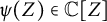 $\psi (Z) \in {\mathbb C}[Z]$
is dominant if
 $|\lambda | \geqslant |\rho |$
for any other root
 $\rho $
of
 $\psi $
. Clearly
 $\psi $
may have up to
 $\deg \psi $
dominant roots. We are mostly interested in the case of one or two dominant roots.
We note the following result which represents a simplified combination of two results (for
 $\nu =1$
and
 $\nu =2$
) of Sha [Reference Sha33, Theorems 1.1 and 1.2].
Lemma 3.3 Let
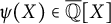 $\psi (X) \in \overline {\mathbb Q}[X]$
be a monic square-free polynomial of degree k and with
 $\nu \leqslant 2$
dominant roots. If
 $\nu =2$
, we also impose that the ratio of the two dominant roots is not a root of unity. Then for any linear recurrence sequence
 $(u_n)_{n=0}^{\infty }$
given by
 $$ \begin{align*} u_n = \sum_{i=1}^k \alpha_i \lambda_i^n , \qquad n \geqslant 0, \end{align*} $$
with characteristic polynomial
 $\psi $
having roots
 $\lambda _i$
,
 $i=1,\ldots ,k$
, if
 $$ \begin{align*} u_n = 0 \end{align*} $$
then
 $$ \begin{align*} n \leqslant \exp\left(C_1 D^4 \left(\max_{i=1, \ldots, k} h\left(\alpha_i\right)+1\right)\right), \end{align*} $$
where
 $C_1$
is an effective constant which depends only on k,
 $D=[{\mathbb K}:{\mathbb Q}]$
is the degree of the smallest Galois field
 ${\mathbb K}$
containing the coefficients of
 $\psi $
and the initial values
 $u_0, \ldots , u_{k-1}$
.
3.4 Zeros of Linear Recurrence Sequences in Families
We now recall a special case of a result of Amoroso et al. [Reference Amoroso, Masser and Zannier2, Theorem 1.5].
Lemma 3.4 Let
 $f_i \in \overline {\mathbb Q}(X)$
,
 $i =1, \ldots , k$
, be nonzero rational functions such that
 $f_s/f_r$
is nonconstant for any
 $1 \leqslant r<s \leqslant k$
. There exists an effectively computable constant
 $C_2$
, which depends on
 $f_1, \ldots , f_k$
such that if for any
 $b_1, \ldots , b_k \in \overline {\mathbb Q}$
not all zero, any
 $n \geqslant C_2$
and any
 $\alpha \in \overline {\mathbb Q}\setminus {\mathfrak E}_{\mathbf {a},\mathbf {f}}$
, one has
 $$ \begin{align*}\sum_{i=1}^k b_i f_i(\alpha)^n = 0, \end{align*} $$
then
 $$ \begin{align*}h(\alpha) \leqslant \frac{k\max\{h(b_1), \ldots,h(b_k) \}}{n}+ C_2. \end{align*} $$
We remark that in [Reference Amoroso, Masser and Zannier2, Theorem 1.5] the bound is given in terms of the height of the projective vector
 $(b_1: \ldots : b_k) \in {\mathbb P}^{k-1}\left (\overline {\mathbb Q}\right )$
which is bounded by the maximum used in Lemma 3.4. Furthermore, in [Reference Amoroso, Masser and Zannier2, Theorem 1.5], only one ratio is assumed to be nonconstant, however, there is an additional request of nonvanishing of subsums in the sum of Lemma 3.4 (under our condition on
 $f_s/f_r$
one can simply consider the shortest vanishing subsum).
We also note that the effectiveness is not explicitly stated in [Reference Amoroso, Masser and Zannier2, Theorem 1.5], however, it is discussed after the formulation of [Reference Amoroso, Masser and Zannier2, Theorem 1.5].
Corollary 3.5 Let
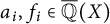 $a_i,f_i \in \overline {\mathbb Q}(X)$
,
 $i =1, \ldots , k$
, be nonzero rational functions such that
 $f_s/f_r$
is nonconstant for any
 $1 \leqslant r<s \leqslant k$
. There exists an effectively computable constant
 $C_3$
, which depends on
 $a_1,\ldots ,a_k,f_1, \ldots , f_k$
such that if for any
 $n\geqslant C_3$
and any
 $\alpha \in \overline {\mathbb Q}$
one has
 $$ \begin{align*}\sum_{i=1}^k a_i(\alpha) f_i(\alpha)^n = 0, \end{align*} $$
then
 $$ \begin{align*}h(\alpha) \leqslant C_3. \end{align*} $$
Proof If
 $\alpha \in {\mathfrak E}_{\mathbf {a},\mathbf {f}}$
, as we have mentioned, this follows from [Reference Silverman36, Theorem 3.11].
We can now assume that
 $\alpha \in \overline {\mathbb Q}\setminus {\mathfrak E}_{\mathbf {a},\mathbf {f}}$
. We can also assume that
 $n> C_2$
, where
 $C_2$
is as in Lemma 3.4, since otherwise
 $\alpha $
is a root of an equation of bounded degree and height.
We now recall that for any
 $\alpha \in \overline {\mathbb Q}$
and
 $a\in \overline {\mathbb Q}(X)$
we have
 $$ \begin{align*} h\left(a(\alpha)\right) \leqslant h\left(\alpha\right) \deg a + C_4, \end{align*} $$
where
 $C_4$
is an effectively computable constant that depends only on a, see [Reference Silverman36, Theorem 3.11]. Hence for
 $$ \begin{align*} n \geqslant 2 k \max\{\deg a_1, \ldots, \deg a_k\} \end{align*} $$
the bound of Lemma 3.4 becomes
 $$ \begin{align*} h(\alpha) & \leqslant \frac{k \max\{h\left((a_1(\alpha)\right), \ldots, h\left(a_k(\alpha)\right)\} }{n}+ C_2\\ & \leqslant \frac{k \max\{\deg a_1, \ldots, \deg a_k\} h\left(\alpha\right) + k C_4}{n}+ C_2\\ & \leqslant \frac{1}{2} h\left(\alpha\right) + C_4/2+ C_2. \end{align*} $$
Hence,
 $h(\alpha )$
is bounded only in terms of
 $a_1, f_1, \ldots , a_k, f_k$
. Choosing
 $$ \begin{align*} C_3= 2k\max\{\deg a_1, \ldots, \deg a_k, C_2\}, \end{align*} $$
the result follows. ▪
3.5 Polynomial ABC Theorem
We need the following generalization [Reference Bombieri and Gubler8, Theorem 12.4.4] of the ABC Theorem for polynomials proved first by Stothers [Reference Stothers39], and then independently by Mason [Reference Mason29] and Silverman [Reference Silverman35]. This is a special case of a more general result for S-units in function fields due to Voloch [Reference Voloch40] and then also Brownawell and Masser [Reference Brownawell and Masser13].
Lemma 3.6 Let
 $g_1,\ldots ,g_m\in \overline {\mathbb Q}[X]$
,
 $m\geqslant 3$
, be such that
 $g_1,\ldots ,g_m$
have no common zero in
 $\overline {\mathbb Q}$
. Assume that
 $$ \begin{align*}g_1(X)+\cdots+g_m(X)=0 \end{align*} $$
and also that no proper subsum
 $$ \begin{align*} \sum_{i \in {\mathcal I}} g_i(X), \qquad \text{with } {\mathcal I} \subseteq \{1, \ldots, m\}, \ 1 \leqslant \#{\mathcal I}< m, \end{align*} $$
vanishes identically. Then
 $$ \begin{align*} \max_{i=1,\ldots,m} \deg g_i\leqslant \frac{(m-1)(m-2)}{2} \max\left\{\deg\mathrm{rad}\left(\prod_{i=1}^m g_i\right)-1,0\right\}. \end{align*} $$
We also need the following result on the multiplicity of roots of certain rational functions, see [Reference Ostafe31, Corollary 2.10]. For a rational function
 $h\in {\mathbb C}(T)$
, we denote by
 $\mathrm {Mult}(h)$
the largest multiplicity of the zeros of h and by
 $Z(h)$
the set of zeros of h in
 ${\mathbb C}$
, respectively.
Lemma 3.7 Let
 $h_i=f_i/g_i$
,
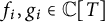 $f_i,g_i\in {\mathbb C}[T]$
,
 $i=1,\ldots ,n$
, with
 $$ \begin{align*} Z(f_1\cdots f_m)\cap Z(g_1\cdots g_m)=\emptyset. \end{align*} $$
Then, for all integers
 $n_1,\ldots ,n_{\ell }\geqslant 0$
and
 $a\in {\mathbb C}^*$
, we have
 $$ \begin{align*} \mathrm{Mult}\left(h_1^{n_1}\cdots h_{\ell}^{n_{m}}-a\right)\leqslant \sum_{i=1}^{m} \left(\deg f_i+\deg g_i\right). \end{align*} $$
3.6 Zeros of Linear Recurrence Sequences in Function Fields
It is well known that the Skolem Problem is settled in the case of linear recurrence sequences over function fields. An effective (but not explicit) bound on the largest zero in such a sequence is given in [Reference Fuchs and Pethö21, Corollary 3.1]. We present it in a simplified form as needed for our setting.
Lemma 3.8 Let
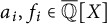 $a_i, f_i \in \overline {\mathbb Q}[X]$
,
 $i =1, \ldots , k$
, be such that
 $f_i/f_j\not \in \overline {\mathbb Q}^*$
for all
 $1\leqslant i< j\leqslant k$
. Let polynomials
 $F_n$
,
 $n\geqslant 1$
, be defined by (1.2). Then there exists an effectively computable constant
 $C_5$
depending on
 $a_i,f_i$
,
 $i=1,\ldots ,k$
, such that if
 $F_n=0$
then
 $n < C_5$
.
We also have the following lower bound on the number of distinct zeros of
 $F_n(X)$
in (1.2).
Lemma 3.9 Let
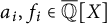 $a_i, f_i \in \overline {\mathbb Q}[X]$
,
 $i =1, \ldots , k$
, be as in Theorem 2.1
and such that
 $\gcd (a_1f_1, \ldots , a_kf_k)=1$
. Then there exists an effective positive constant
 $C_6$
depending only on
 $a_i,f_i$
,
 $i=1,\ldots ,k$
, such that for any
 $n\geqslant C_6$
, the polynomial
 $F_n$
defined by (1.2) has at least
 $$ \begin{align*}\frac{2}{k(k-1)} \max_{i=1,\ldots, n} \{\deg a_i +n\deg f_i\} -2dk \end{align*} $$
distinct roots.
Proof Let
 $C_5$
be as in Lemma 3.8. Then, for any
 $n\geqslant C_5$
we know that
 $F_n\ne 0$
. We consider now the equation
 $$ \begin{align} F_n(X)-\sum_{i=1}^k a_i(X)f_i(X)^n =0. \end{align} $$
We also note that for
 $n\geqslant C_5$
no subsum of the terms from the set
 $$ \begin{align*}\left\{F_n(X), a_1(X)f_1(X)^n, \ldots, a_k(X)f_k(X)^n\right\} \end{align*} $$
vanishes identically. Indeed, if this happens, then there is a proper subset
 ${\mathcal I}\subseteq \{1,\ldots ,k\}$
such that
 $$ \begin{align*}\sum_{i\in {\mathcal I}} a_i(X)f_i(X)^n=0. \end{align*} $$
Since
 $n\geqslant C_5$
, this contradicts Lemma 3.8.
Let
 ${\mathcal S}_n$
be the set of all distinct zeros of
 $F_n$
. We can now apply Lemma 3.6 to (3.1) to conclude that
 $$ \begin{align*}\max_{i=1,\ldots, k} \{\deg a_i +n\deg f_i\}\leqslant \frac{k(k-1)}{2}\left(\# {\mathcal S}_n +\sum_{i=1}^k (\deg a_i +\deg f_i)\right). \end{align*} $$
From here we obtain
 $$ \begin{align*}\# {\mathcal S}_n \geqslant \frac{2\max_{i=1,\ldots, k} \{\deg a_i +n\deg f_i\}}{k(k-1)} -2dk, \end{align*} $$
which concludes the proof (with
 $C_6 = C_5$
). ▪
Remark 3.10 We note that under a more restrictive condition that the k products
 $a_1f_1, \ldots , a_kf_k$
are pairwise relatively prime, one can take
 $C_6=1$
in Lemma 3.9. Furthermore, under the more restrictive condition that
 $2k$
polynomials
 $a_1, f_1, \ldots , a_k, f_k$
are pairwise relatively prime, one can also use the result of Brindza [Reference Brindza12, Theorem 1] to show that the polynomial
 $F_n$
has at least
 $n/(k-1)-(d+1)k$
distinct roots.
We also remark that a tight lower bound for the degree of
 $F_n$
has recently been given in [Reference Fuchs and Heintze20, Corollary 2] (in fact for arbitrary nondegenerate linear recurrences including nonsimple ones).
3.7 Characterization of Linear Recurrence Sequences
To test whether an arbitrary sequence
 $ (v_n)_{n=1}^{\infty }$
of elements of a field
 ${\mathbb F}$
is a linear recurrence sequence, we recall the following well-known result which is based on the vanishing of the Kronecker–Hankel determinants
 $$ \begin{align} \Delta_{h}=\det \left(v_{i+j}\right)_{0\leqslant i,j \leqslant h-1}. \end{align} $$
More precisely, by [Reference Lidl and Niederreiter28, Theorem 8.75] (see also [Reference Everest, van der Poorten, Shparlinski and Ward18, Theorem 1.6] and [Reference Koblitz23, Lemma 5, Chapter V] for variations) we have:
Lemma 3.11 A sequence
 $(v_n)_{n=1}^{\infty }$
of elements of a field
 ${\mathbb F}$
is a linear recurrence sequence of order k if and only if for the determinants (3.2) we have
 $\Delta _{h} =0$
for all
 $h\geqslant k+1$
.
4 Proofs of Results Toward the Skolem Problem
4.1 Proof of Theorem 2.1
Multiplying by common denominators of
 $a_i(X)$
and of
 $f_i(X)$
,
 $i =1, \ldots , k$
, we can assume that
 $a_i(X), f_i(X) \in \overline {\mathbb Q}[X]$
,
 $i =1, \ldots , k$
.
Let
 $\alpha \in \overline {\mathbb Q} \setminus {\mathfrak E}_{\mathbf {a},\mathbf {f}}$
be such that (2.3) holds.
We now consider the case when we have at least three dominant roots, that is, there exist distinct integers
 $1 \leqslant r< s < t \leqslant k$
such that
 $$ \begin{align*}|f_r(\alpha)|=|f_s(\alpha)|=|f_t(\alpha)|, \end{align*} $$
or equivalently,
 $$ \begin{align*}\frac{|f_s(\alpha)|}{|f_r(\alpha)|}=\frac{|f_t(\alpha)|}{|f_r(\alpha)|}=1. \end{align*} $$
Since by hypothesis,
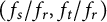 $(f_s/f_r,f_t/f_r)$
is a nonexceptional rational function, from Lemma 3.1 we see that for each of the
 $k(k-1)(k-2)/6$
possible choices of the triple
 $(r,s,t)$
there are at most
 $4d^2$
such
 $\alpha \in \overline {\mathbb Q}$
.
Hence in total we have excluded at most
 $$ \begin{align} 4d^2 k(k-1)(k-2)/6 = 2d^2 k(k-1)(k-2)/3 \end{align} $$
elements
 $\alpha \in \overline {\mathbb Q} \setminus {\mathfrak E}_{\mathbf {a},\mathbf {f}}$
.
We thus assume that we have at most two dominant roots. In this case, we apply Lemma 3.3 to any element
 $\alpha \in \overline {\mathbb Q}\setminus {\mathfrak E}_{\mathbf {a},\mathbf {f}}$
and derive that
 $$ \begin{align*}n \leqslant \exp\left(C_7 D^4_{\alpha} (h(\alpha)+1)\right), \end{align*} $$
for an effectively computable constant
 $C_7$
, which depends only on
 $a_1,\ldots ,a_k,f_1, \ldots , f_k$
. We now observe that for
 $n\leqslant C_3$
, where
 $C_3$
is as in Corollary 3.5, the result is trivial. Otherwise Corollary 3.5 applies and we obtain the desired result.
4.2 Proof of Corollary 2.3
By Theorem 2.1 we only need to estimate the number
 $R(D)$
of roots of unity of degree at most D over
 ${\mathbb Q}$
. Clearly
 $$ \begin{align*} R(D) = \sum_{m:\varphi(m) \leqslant D} \varphi(m) \leqslant D \sum_{m:\varphi(m) \leqslant D} 1, \end{align*} $$
where
 $\varphi (m)$
is the Euler function. Using the bound
 $$ \begin{align*}\sum_{m:\varphi(m) \leqslant D} 1 \leqslant 23 D \end{align*} $$
of Dubickas and Sha [Reference Dubickas and Sha17, Lemma 4.1], we see that
 $$ \begin{align} R(D) \leqslant 23 D^2 \end{align} $$
(using partial summation one can certainly obtain a tighter bound). Now, since each of
 $k(k-1)/2$
ratios
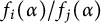 $f_i(\alpha )/f_j(\alpha )$
can be a root of unity of degree at most D, there are at most
 $$ \begin{align*}dR(D) \frac{k(k-1)}{2} < 12 dD^2k^2 \end{align*} $$
such
 $\alpha \in {\mathcal A}_D$
, which we need to exclude.
Taking into account that we also need to exclude at most other
 $2d^2 k(k-1) (k-2)/3$
elements
 $\alpha \in {\mathcal A}_D$
as in Theorem 2.1, and at most
 $2dk$
zeros of
 $a_i, f_i$
,
 $i=1,\ldots ,k$
, and thus at most
 $$ \begin{align*}2d^2 k(k-1)(k-2)/3+2dk \leqslant 2d^2k^3/3 \end{align*} $$
elements (elementary calculus show that the last inequality holds for any
 $d \geqslant 1$
and
 $k\geqslant 2$
). Hence, we conclude the proof.
4.3 Proof of Corollary 2.4
Let
 ${\mathbb K}$
be a number field with
 $[{\mathbb K}:{\mathbb Q}]=D$
such that
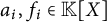 $a_i,f_i\in {\mathbb K}[X]$
,
 $i=1,\ldots ,k$
.
Let
 $\alpha \not \in {\mathfrak E}_{\mathbf {a},\mathbf {f}}$
be a root of
 $F_n$
for some
 $n\geqslant 1$
. Let G be its minimal polynomial over
 ${\mathbb K}$
, which implies that
 $G\mid F_n$
. Let
 $D_G=\deg G=[{\mathbb K}(\alpha ):{\mathbb K}]$
and let
 ${\mathbb M}_{\alpha }$
be the smallest Galois extension of
 ${\mathbb Q}$
which includes
 ${\mathbb K}(\alpha )$
.
For any
 $\sigma \in {\mathrm {Gal}}({\mathbb K}(\alpha )/{\mathbb K})$
, conjugating the relation
 $F_n(\alpha )=0$
gives us
 $$ \begin{align} \sum_{i=1}^k a_i(\sigma(\alpha)) f_i(\sigma(\alpha))^n=0. \end{align} $$
We may assume that
 $D_G>2d^2k^3/3$
. Indeed, if
 $D_G\leqslant 2d^2k^3/3$
, then
 $$ \begin{align*}[{\mathbb K}(\alpha):{\mathbb Q}]\leqslant DD_G \leqslant \frac{2}{3} Dd^2k^3, \end{align*} $$
and since by Corollary 3.5,
 $h(\alpha )$
is bounded from the above by a constant depending only on
 $a_1, f_1, \ldots , a_k, f_k$
, by Northcott’s theorem there are finitely many such
 $\alpha $
. Thus, we can exclude the irreducible factors of
 $F_n$
,
 $n\geqslant 1$
, corresponding to these finitely many elements.
Now, since there are
 $D_G>2d^2k^3/3$
distinct elements
 $\sigma (\alpha )$
satisfying (4.3), and taking into account the hypothesis on the polynomials
 $f_i$
, we can apply Theorem 2.1 to conclude that there exists
 $\sigma \in {\mathrm {Gal}}({\mathbb K}(\alpha )/{\mathbb K})$
such that (4.3) holds and for which
 $$ \begin{align*}n\leqslant \exp\left(C_8[{\mathbb M}_{\alpha}:{\mathbb Q}]^4\right) \end{align*} $$
for some constant
 $C_8$
which depends only on
 $a_1, f_1, \ldots , a_k, f_k$
. This concludes the proof.
4.4 Proof of Corollary 2.5
Let the set
 ${\mathcal E}$
be as in Corollary 2.4. Clearly, if
 $F_n$
has a root outside of the set
 ${\mathcal E} \cup {\mathfrak E}_{\mathbf {a},\mathbf {f}}$
the result is instant from Corollary 2.4.
Otherwise, since
 ${\mathcal E}$
is a finite set and so are the sets of
 $\alpha \in \overline {\mathbb Q}$
with
 $f_i(\alpha )=0$
or
 $a_i(\alpha )=0$
, for some
 $1 \leqslant i \leqslant k$
, adjusting the constant
 $c_0$
we can make the desired result valid for these values of
 $\alpha $
as well.
Hence, it remains to consider the case when the ratio
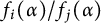 $f_i(\alpha )/f_j(\alpha )$
is a root of unity for some
 $1 \leqslant i <j\leqslant k$
. We recall that by Lemma 3.9,
 $F_n$
has at least
 $2n/k(k-1) - C_9$
distinct roots
 $\alpha $
, for some constant
 $C_9$
which depends only on
 $a_1, f_1, \ldots , a_k, f_k$
. By our assumption, for each of them at least one ratio
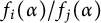 $f_i(\alpha )/f_j(\alpha )$
is a root of unity for some
 $1 \leqslant i <j\leqslant k$
. For each
 $\gamma \in \overline {\mathbb Q}$
the equation
 $f_i(\alpha )/f_j(\alpha ) = \gamma $
has at most d solutions
 $\alpha \in \overline {\mathbb Q}$
. Hence, the set of roots of unity among the ratios
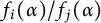 $f_i(\alpha )/f_j(\alpha )$
form a set
 ${\mathcal U}_{\mathbf {f}}$
of at least
 $$ \begin{align*}\# {\mathcal U}_{\mathbf{f}} \geqslant 2n/dk(k-1) - C_9/d \end{align*} $$
distinct roots of unity
 $\rho $
for some
 $1 \leqslant i <j\leqslant k$
.
Recall the bound (4.2) on the number of roots of unity of degree at most D. Hence, at least one of the above roots of unity is of degree at least
 $$ \begin{align*}\sqrt{ \frac{1}{23}\# {\mathcal U}_{\mathbf{f}}} \geqslant\sqrt{ \frac{2n}{23dk(k-1)} - C_9/23d}. \end{align*} $$
and thus so is
 $\alpha $
. Hence in this case we have a much stronger bound than claimed.
5 Proof of Theorem 2.7 on Perfect Powers in Specializations at Roots of Unity
Let
 ${\mathbb K}$
be the field of definition of the polynomials
 $a_i, f_i$
. Thus,
 $a_i,f_i\in {\mathbb Z}_{\mathbb K}[X]$
, where
 ${\mathbb Z}_{\mathbb K}$
is the ring of integers of
 ${\mathbb K}$
.
As we have shown in the proof of Theorem 2.1, see (4.1), for all but at most
 $2d^2k^3/3$
elements
 $\alpha \in {\mathbb U} \setminus {\mathfrak E}_{\mathbf {a},\mathbf {f}}$
, the sequence
 $\left (F_n(\alpha )\right )_{n=1}^{\infty }$
has at most two dominant roots.
Let us assume first that for such an element
 $\alpha \in {\mathbb U} \setminus {\mathfrak E}_{\mathbf {a},\mathbf {f}}$
, the sequence
 $\left (F_n(\alpha )\right )_{n=1}^{\infty }$
has two dominant roots, that is, for some
 $1\leqslant i\ne j\leqslant k$
,
 $|f_i(\alpha )|=|f_j(\alpha )|$
. This implies that
 $$ \begin{align} f_i(\alpha)\overline{f_i}(\overline\alpha) = f_i(\alpha)\overline{ f_i(\alpha)} =f_j(\alpha)\overline{f_j(\alpha) } =f_j(\alpha)\overline{f_j}(\overline\alpha), \end{align} $$
where
 $\overline \alpha $
is the complex conjugate of
 $\alpha $
, which is again a root of unity.
Since by our assumption,
 $$ \begin{align*} f_i(X)\overline{f_i}(Y) - f_j(X)\overline{f_j}(Y)\in{\mathbb K}[X,Y], \qquad 1\leqslant i\ne j\leqslant k, \end{align*} $$
do not have any factor of the form
 $X^rY^s-u$
or
 $X^r-uY^s$
with
 $u \in {\mathbb U}$
, by a result of Lang [Reference Lang25], we know that there are finitely many solutions
 $(\alpha ,\beta )$
in roots of unity (and thus also of the form
 $(\alpha ,\overline {\alpha })$
) to the equation (5.1). Moreover, by [Reference Beukers and Smyth6, Section 4.1], the equation
 $$ \begin{align*} f_i(X)\overline{f_i}(Y) - f_j(X)\overline{f_j}(Y)=0 \end{align*} $$
has at most
 $44d^2$
solutions
 $(\alpha ,\beta )$
in roots of unity. Thus, there are at most
 $22d^2k (k-1)< 22d^2k^2$
such elements
 $\alpha \in {\mathbb U} \setminus {\mathfrak E}_{\mathbf {a},\mathbf {f}}$
such that the sequence
 $\left (F_n(\alpha )\right )_{n=1}^{\infty }$
has two dominant roots.
Thus, for all but
 $d^2(2k^3/3 + 22k^2)$
elements
 $\alpha \in {\mathbb U} \setminus {\mathfrak E}_{\mathbf {a},\mathbf {f}}$
, the sequence
 $\left (F_n(\alpha )\right )_{n=1}^{\infty }$
has only one dominant root. Let such an element
 $\alpha \in {\mathbb U} \setminus {\mathfrak E}_{\mathbf {a},\mathbf {f}}$
. We now apply the result of Fuchs [Reference Fuchs19, Corollary 2.10] describing the structure of the set of perfect powers in linear recurrent sequences over number fields (one easily verifies that for
 $\alpha \in {\mathbb U} \setminus {\mathfrak E}_{\mathbf {a},\mathbf {f}}$
all necessary conditions of [Reference Fuchs19, Corollary 2.10] are satisfied). This concludes the proof.
6 Proofs of Results on Common Zeros
6.1 Proof of Theorem 2.9
For given
 $\mathbf {m}=(m_1,\ldots ,m_r)$
,
 $\mathbf {n}=(n_1,\ldots ,n_s)$
, and
 $u,v\in \Gamma ^{\mathrm {div}}$
, we define
 $$ \begin{align*}{\mathcal D}_{\mathbf{m},\mathbf{n},u,v}(X)=\gcd\left(\prod_{i=1}^rf_i(X)^{m_i}-u,\prod_{j=1}^sg_j(X)^{n_j}-v \right). \end{align*} $$
We recall that by the greatest common divisor of two rational functions we mean the greatest monic common divisor of their numerators. In particular,
 ${\mathcal D}_{\mathbf {m},\mathbf {n},u,v}\in \overline {\mathbb Q}[X]$
.
The proof follows the same approach as in the proof of [Reference Ostafe31, Theorem 1.3]. Indeed, since the rational functions
 $f_1,\ldots ,f_r,g_1,\ldots ,g_s$
are multiplicatively independent modulo
 $\Gamma $
, by Lemma 3.2, applied with
 $n=r+s$
and
 $$ \begin{align*} &(k_1,\ldots,k_n)= (m_1,\ldots,m_r, 0, \ldots, 0),\cr &(\ell_1,\ldots,\ell_n) = (0, \ldots, 0, n_1,\ldots,n_s), \end{align*} $$
there are finitely many
 $\alpha \in \overline {\mathbb Q}$
such that
 ${\mathcal D}_{\mathbf {m},\mathbf {n},u,v}(\alpha )=0$
for some nonzero integer vectors
 $\mathbf {m},\mathbf {n}$
as above and
 $u,v\in \Gamma ^{\mathrm {div}}$
. We denote this finite set, depending only on
 $f_i,g_j$
, by
 ${\mathcal S}$
.
To construct the polynomial h we need to control also the multiplicity of the roots of the polynomials
 ${\mathcal D}_{\mathbf {m},\mathbf {n},u,v}$
. This is also readily given by Lemma 3.7, which implies that
 $$ \begin{align*}\mathrm{Mult}({\mathcal D}_{\mathbf{m},\mathbf{n},u,v}) \leqslant 2\min\left\{\sum_{i=1}^r\deg f_i ,\, \sum_{j=1}^s \deg g_j\right\}. \end{align*} $$
Thus, we can define the polynomial
 $h\in \overline {\mathbb Q}[X]$
by
 $$ \begin{align*}h(X)=\prod_{\gamma\in{\mathcal S}} (X-\gamma)^{2\min\left\{\sum_{i=1}^r\deg f_i ,\, \sum_{j=1}^s \deg g_j\right\}}, \end{align*} $$
which concludes the proof.
6.2 Proof of Corollary 2.11
Let
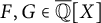 $F,G\in \overline {\mathbb Q}[X]$
be of degree at most
 $d\geqslant 1$
with all roots in
 $\Gamma ^{\mathrm {div}}$
. We reduce the problem to looking at each greatest common divisor
 $$ \begin{align*}\gcd\left(\prod_{i=1}^rf_i(X)^{m_i}-\gamma_1,\prod_{j=1}^sg_j(X)^{n_j}-\gamma_2\right) \end{align*} $$
with roots
 $\gamma _1$
and
 $\gamma _2$
of F and G, respectively and
 $(m_1,\ldots ,m_r)\in {\mathbb N}^r\setminus \{{\mathbf 0}\}$
,
 $(n_1,\ldots ,n_s)\in {\mathbb N}^s\setminus \{{\mathbf 0}\}$
.
By Theorem 2.9, there exists a polynomial
 $h\in \overline {\mathbb Q}[X]$
that depends only on
 $f_i,g_j$
and the generators of
 $\Gamma $
such that for all
 $(m_1,\ldots ,m_r)\in {\mathbb N}^r\setminus \{{\mathbf 0}\}$
,
 $(n_1,\ldots ,n_s)\in {\mathbb N}^s\setminus \{{\mathbf 0}\}$
and
 $\gamma _1,\gamma _2\in \Gamma ^{\mathrm {div}}$
one has
 $$ \begin{align*}\gcd\left(\prod_{i=1}^r f_i(X)^{m_i}-\gamma_1,\prod_{j=1}^sg_j(X)^{m_j}-\gamma_2\right)\mid h. \end{align*} $$
Since both F and G have at most d roots in
 $\Gamma ^{\mathrm {div}}$
, we conclude the proof choosing
 $H=h^{d^2}$
.
7 Proof of Theorem 2.12
For each
 $\alpha \in {\mathbb C}$
, we consider the sequence
 $\left (\Delta _h(\alpha )\right )_{h=0}^{\infty }$
of Kronecker–Hankel determinants
 $$ \begin{align*}\Delta_h(\alpha)=\det\left(F_{i+j}(\alpha)\right)_{0\leqslant i,j\leqslant h-1}, \quad h=0,1,\ldots. \end{align*} $$
Assume that there exist infinitely many
 $\alpha \in {\mathbb C}$
such that
 $\left (F_n(\alpha )\right )_{n=0}^{\infty }$
is a linear recurrence of order at most K. Hence, be Lemma 3.11 for all
 $h\geqslant K+1$
we have
 $$ \begin{align*}\Delta_h(\alpha)=0 \end{align*} $$
for infinitely many
 $\alpha \in {\mathbb C}$
. Therefore, for all
 $h\geqslant K+1$
, the rational function
 $$ \begin{align*}\Delta_h(X)=\det\left(F_{i+j}(X)\right)_{0\leqslant i,j\leqslant h-1} \end{align*} $$
has infinitely many zeros, and thus is identical to zero.
Applying Lemma 3.11 again, we conclude the proof.
8 Comments and Further Questions
As we have mentioned Theorem 2.1 can be extended to nonsimple sequences without new ideas and just at the cost of introducing more complicated notations.
We also remark that Theorem 2.1 is an analogue of a result of Kulkarni et al. [Reference Kulkarni, Mavraki and Nguyen24, Proposition 2.2], see also [Reference Bell, Nguyen and Zannier4, Proposition 2.2], in which the coefficients
 $a_1, \ldots , a_k$
of
 $F_n(X)$
in (1.2) are constants rather than rational functions as in our case. Moreover, [Reference Kulkarni, Mavraki and Nguyen24, Proposition 2.2] is not effective while Theorem 2.1 is.
Furthermore, if as in [Reference Kulkarni, Mavraki and Nguyen24] the coefficients
 $a_1, \ldots , a_k$
of
 $F_n(X)$
in (1.2) are constants then analyzing the bounds of [Reference Sha33] underlying Lemma 3.3, we see that
 $D^4$
can be replaced with
 $D_0^3D$
, where
 $D_0$
is the degree of the Galois closure of
 ${\mathbb Q}(a_1, \ldots , a_k)$
over
 ${\mathbb Q}$
. In turn, in this case, this leads to a single exponential bound of the form
 $$ \begin{align*}n \leqslant \exp\left(C D_{\alpha}\right), \end{align*} $$
in Theorem 2.1.
We describe a possible generalization of Theorem 2.1 to S-unit equations in
 $\overline {\mathbb Q}(X)$
. Let
 $\Gamma $
be a finitely generated subgroup of
 $\overline {\mathbb Q}(X)$
and fix rational functions
 $a_1,\ldots ,a_k\in \overline {\mathbb Q}(X)$
. By [Reference Amoroso, Masser and Zannier2, Proposition 6.1], for any rational functions
 $u_1,\ldots ,u_k\in \Gamma $
such that
 $$ \begin{align*}u_i/u_j \not \in \overline{\mathbb Q}, \quad 1\leqslant i <j\leqslant k, \qquad\text{ and}\qquad \sum_{i=1}^k a_iu_i\ne 0, \end{align*} $$
the set of
 $\alpha \in \overline {\mathbb Q}$
such that
 $$ \begin{align} \sum_{i=1}^k a_i(\alpha)u_i(\alpha)=0 \end{align} $$
is a set of bounded height, depending only on
 $a_1,\ldots ,a_k$
and the generators of
 $\Gamma $
.
We now ask for an analogue of Theorem 2.1 for such equations. It is convenient to define the notion of a primitive solution to (8.1) as a solution with
 $u_i(\alpha ) = 1$
for some
 $i = 1, \ldots , k$
.
We now ask the following.
Question 8.1 Is it true, under some natural conditions on the generators of
 $\Gamma $
, that outside of a set of bounded height of values
 $\alpha \in \overline {\mathbb Q}$
, then for every primitive solution to (8.1),
 $\max _{i=1,\ldots ,k}\deg u_i$
is bounded only in terms of the degree
 $D_{\alpha }$
of the smallest Galois field
 ${\mathbb K}$
over
 ${\mathbb Q}$
with
 $\alpha \in {\mathbb K}$
, the functions
 $a_1,\ldots ,a_k$
and the generators of
 $\Gamma $
?
We note that the idea of the proof of [Reference Amoroso, Masser and Zannier2, Proposition 6.1] which reduces S-unit equations to equations of the type (2.3), can perhaps help to tackle Question 8.1. Unfortunately, during this reduction we do not control well the corresponding polynomials
 $a_1,f_1,\ldots ,a_k,f_k \in \overline {\mathbb Q}(X)$
and in particular it is not immediately clear how to verify the necessary condition of Theorem 2.1.
We remark that the proof of Theorem 2.1 relies on the fact that outside of a small set of parameters the corresponding specializations are sequences with at most two dominant roots. On the other hand, in the proof of Theorem 2.7 we show that for all but finitely many specializations at roots of unity these sequences have only one dominant root. These ideas can be used to study many other properties of the corresponding linear recurrence sequences. For example, by combining this approach with results and ideas of [Reference Shparlinski34, Reference Stewart37, Reference Stewart38] one can study prime ideal divisors of elements of these sequences.
Acknowledgments
The authors would like to thank Umberto Zannier for useful discussions on previous versions of the file. The authors are also very grateful to the referee for the very helpful comments.
This work was supported, in part, by the Australian Research Council Grants DP180100201 and DP200100355. The first author gratefully acknowledges the hospitality and generosity of the Max Planck Institute of Mathematics, where parts of this paper were developed.



