





1 Introduction
1.1 Context, motivations, and contributions of this paper
The enumeration of maps is a classical topic in combinatorics, which was initiated by Tutte in the sixties, and which has seen many developments up to now. See for instance the review by Schaeffer [Reference Schaeffer54] and the references cited therein. Let us also mention the book by Lando and Zvonkin [Reference Lando and Zvonkin50] which provides an overview of some fascinating connections between map enumeration and other branches of mathematics, involving avatars of maps such as dessins d’enfants and combinatorial models of the moduli space of complex curves.
A paradigmatic problem in map enumeration is to count planar maps while controlling face degrees. This question was first considered by Tutte [Reference Tutte58] who obtained a remarkably simple expression when all degrees are even. In the general case, he obtained a functional equation for the corresponding generating function [Reference Tutte59], whose solution was given by Bender and Canfield [Reference Bender and Rodney Canfield8], see also [Reference Bousquet-Mélou and Jehanne17]. Independently, the same problem was solved in theoretical physics in connection with the so-called one-matrix model, see, for example, [Reference Di Francesco, Ginsparg and Zinn-Justin34, Reference Bouttier18] and references therein.
While these approaches lead to an explicit answer, in the form of generating functions amenable to an asymptotic analysis, it is natural to look for a bijective approach. Such an approach was pioneered by Schaeffer who rederived Tutte’s result in the case of even degrees [Reference Schaeffer53], and later extended to arbitrary degrees by Bouttier, Di Francesco and Guitter [Reference Bouttier, Di Francesco and Guitter19]. Both papers rely on correspondences between planar maps and certain decorated trees, often called blossom(ing) trees. Another bijection, involving another family of trees known as mobiles, was given in [Reference Bouttier, Di Francesco and Guitter20].
Trees are easier to enumerate thanks to their recursive structure: for rooted trees, the operation of removing the root vertex translates into equations – that are typically algebraic – determining their generating functions. This naturally raises the question of whether such recursive decompositions can be performed directly at the level of maps. A construction of this type was proposed in [Reference Bouttier and Guitter22, Appendix A], and is now known as the slice decomposition, see also [Reference Bouttier23, Chapter 2] and [Reference Bouttier, Guitter and Miermont27]. It provides an elementary yet elegant bijective solution to the problem of counting maps with controlled face degrees, and moreover extends naturally to maps with girth constraints [Reference Bouttier and Guitter21, Reference Bouttier, Guitter and Manet26] and to scaling limits [Reference Bettinelli and Miermont13].
In this paper, we extend the slice decomposition to the more general context of planar hypermaps. Recall that a hypergraph generalizes a graph by allowing hyperedges, which may be incident to an arbitrary number of vertices rather than just two. A hypermap is the generalization of a map in the same manner. In practice, we represent hyperedges as faces of a second color, so that hypermaps are identified with properly face-bicolored maps, dual to bipartite maps [Reference Walsh60]. Let us mention that slice decompositions for particular instances of hypermaps, namely constellations and corner triangulations, have been considered previously in [Reference Albenque and Bouttier1] and [Reference Dervieux32, Reference Dervieux, Poulalhon and Schaeffer33] respectively.
The above paradigmatic enumeration problem extends naturally to hypermaps: it consists in counting planar hypermaps while controlling the degrees of both faces and hyperedgesFootnote 1 or, in the representation chosen in this paper, the degrees of faces of each color separately. This indeed generalizes the previous problem, since maps correspond to hypermaps in which all hyperedges have degree two. The question seems to have been first addressed in the physics literature in connection with the two-matrix model [Reference Itzykson and Zuber46, Reference Mehta52, Reference Douglas37, Reference Staudacher56, Reference Daul, Kazakov and Kostov31]. A key motivation for physicists was the study of two-dimensional quantum gravity [Reference Di Francesco, Ginsparg and Zinn-Justin34], as it was realized that the two-matrix model exhibits a much richer critical behavior than the one-matrix model. In other words, generating functions for planar hypermaps with controlled degrees display certain types of singularities that cannot be obtained with planar maps only. In particular, a specialization of the two-matrix model is the celebrated Ising model on (dynamical) random planar maps, first solved by Kazakov [Reference Kazakov47], which remarkably displays a phase transition and a critical point [Reference Boulatov and Kazakov15]. The deep algebraic and integrable structures underpinning the two-matrix model were further investigated, in particular by Bertola, Eynard and their collaborators, see, for example, [Reference Bertola12, Reference Eynard41, Reference Eynard and Orantin39] and references therein. We refer to the eighth chapter of the book [Reference Eynard40] for a combinatorially oriented account of some of these resultsFootnote 2 . Let us mention in passing the recent works [Reference Duits, Hayford and Lee38, Reference Hayford45] on a Riemann-Hilbert approach to the two-matrix model and its application to the Ising model coupled to 2D gravity.
On the bijective side, the first approach to the problem of counting degree-controlled hypermaps was made by Bousquet-Mélou and Schaeffer [Reference Bousquet-Melou and Schaeffer16] via blossoming trees (and in the dual setting of bipartite maps), thereby confirming rigorously the prediction of Boulatov and Kazakov for the genus 0 partition function of the Ising model on random tetravalent planar maps. Another bijective approach via mobiles was given in [Reference Bouttier, Di Francesco and Guitter20, Section 3]Footnote
3
. These two approaches give systems of recursive equations which are equivalent to those obtained for slices in the present paper, see Remarks 2.16 and 2.20 below. Their limitation, however, was that the bijections imposed somewhat “unnatural” constraints on the trees or maps. Namely, the main result of Bousquet-Mélou and Schaeffer [Reference Bousquet-Melou and Schaeffer16, Theorem 3] is about maps rooted at a black vertex of degree
 $2$
, and it was unclear whether this restriction could be lifted. And the construction given in [Reference Bouttier, Di Francesco and Guitter20, Section 3.3] produces mobiles whose labels are constrained to be positive, which complicates their enumeration considerably. Such issues were typical in the early days of the bijective approach to map enumeration, and were later addressed by lifting the balance condition in blossoming trees (using
 $\alpha $
-orientations), or by considering pointed rooted maps to relax positivity in mobiles, etc. Modern treatments of tree bijections for hypermaps can be found in [Reference Bernardi and Fusy11] and [Reference Albenque, Ménard and Tokka4]: the first paper discusses a very general bijection for hypermaps with girth constraints, and recovers [Reference Bousquet-Melou and Schaeffer16, Reference Bouttier, Di Francesco and Guitter20] as special cases; the second paper introduces a family of orientations characterizing bipartite maps (dual to hypermaps) which allows to recover and extend the blossoming bijection of [Reference Bousquet-Melou and Schaeffer16]. Still, to the best of our knowledge, most of the nice enumerative results from [Reference Eynard40, Chapter 8] have not yet received a bijective proof, and this is the gap that we intend to address with this paper.
We will show that the slice framework is particularly well-suited for this purpose: slices are certain (hyper)maps that admit recursive decompositions equivalent to those of blossoming trees and mobiles, while also serving as building blocks to construct bijectively several “natural” families of hypermaps. Let us list, by increasing order of complexity, which families we treat in the paper: pointed disks with one monochromatic boundary, cylinders with two monochromatic boundaries (starting with the case of so-called trumpets and cornets, that is, cylinders with one geodesic boundary)Footnote 4 , disks with one monochromatic boundary, disks with a “Dobrushin” boundary condition. The case of more general “mixed” boundary conditions, discussed in [Reference Eynard40, Section 8.4], is not treated in the present paper, but will be adressed in future works [Reference Bouttier, Eynard and Lejeune25, Reference Lejeune51].
Another contribution of the present paper is a combinatorial explanation for the existence of a “rational parametrization” for the generating functions of hypermaps with monochromatic boundaries, in terms of the parameters controlling the boundary lengths. This phenomenon was previously observed in the approach via loop equations, see, for example, [Reference Eynard40, Section 8.3], but its origin remained mysterious to us. One of our insights is that hypermaps with monochromatic boundaries can be ultimately decomposed as sequences of slices whose increments form downward skip-free (Łukasiewicz-type) walks. Generating functions for such sequences/walks can all be expressed in terms of a single “master” series, which is the generating function of excursions. See Appendix A below for a self-contained discussion. In our application to hypermaps we actually have two master series, one per color, and the variable controlling the length of a boundary of a given color turns out to be a Laurent polynomial in the corresponding master series.
Let us mention that one of our main motivations is the aforementioned Ising model on random maps, which is expected to display at the critical point large-scale geometric properties that are totally different from those of generic maps. A probabilistic approach to this model was recently developed in the papers [Reference Albenque, Ménard and Schaeffer3, Reference Albenque and Ménard2, Reference Chen and Turunen28, Reference Chen and Turunen29, Reference Turunen57], which rely heavily on enumerative results such as those given in [Reference Bernardi and Bousquet-Mélou10, Section 12]Footnote
5
. It is conjectured that the scaling limit, in the Gromov-Hausdorff sense, of random planar maps coupled to the critical Ising model and endowed with the graph metric is described by the
 $\gamma $
-Liouville quantum gravity metric at
 $\gamma =\sqrt {3}$
[Reference Ding, Dubédat and Gwynne36]. This remains a major open question, and in fact even the value of the scaling factor/Hausdorff dimension
 $d_\gamma $
remains unknown. A possible way to address this question would be to use the method of peeling, and in particular metric growths [Reference Curien30]. Applying this approach to the Ising model requires combinatorial results that are unavailable at the moment. We hope that the present paper might help to make progress in that direction.
Finally, let us note that some of the ideas developed here have already been applied in [Reference Bonzom14] to the enumeration of certain planar constellations, corresponding to the spectral curve of Orlov–Scherbin
 $2$
-Toda tau functions.
The remainder of this introduction delves into the matter, first by giving some precise definitions, then by giving an overview of the enumerative results which will follow from our bijective approach, and finally by presenting the outline of the rest of the paper.
1.2 Maps and hypermaps: basic notions and definitions
Let us now introduce precisely the objects which we intend to enumerate in this paper. We start with some basic notions on maps, and refer to [Reference Schaeffer54] for more details.
A planar map, hereafter called map for short, is a proper embedding of a connected finite multigraph into the sphere, considered up to orientation-preserving homeomorphism. By multigraph, we mean a graph where loops and multiple edges are allowed. A map consists of vertices, edges, faces, and their incidence relations. The embedding fixes the cyclical order of edges around each vertex, which defines readily a corner as a couple of consecutive edges around a vertex. The set of vertices, edges, faces and corners of a planar map
 $\text {m}$
are respectively denoted by
 $\text {V}(\text {m})$
,
 $\text {E}(\text {m})$
,
 $\text {F}(\text {m})$
and
 $\text {C}(\text {m})$
. For any
 $\kappa \in \text {C}(\text {m})$
, the vertex incident to
 $\kappa $
is denoted by
 ${\text {v}}(\kappa )$
. A corner is also incident to a unique face.
The degree of a vertex or a face is defined as the number of its incident corners. In other words, it counts incident edges, with multiplicity 2 for each loop (in the case of vertex degree) or for each bridge (in the case of face degree). The contour of a face is the cycle formed by its incident edges and vertices.
A boundary is a distinguished face. Unless otherwise stated, each boundary is rooted, that is, it is endowed with a marked incident corner. Faces which are not boundaries are called inner faces. Planar maps with one and two boundaries are colloquially called disks and cylinders, respectively. It is customary to draw a planar map in the plane, upon performing a stereographic projection of the sphere. This requires choosing a point at infinity, usually within a face which is therefore promoted to the role of outer (unbounded) face. In a map with boundaries, the outer face is chosen among the boundaries. Note that the other boundaries are not called inner faces in our present terminology.
In this paper, we consider hypermaps, that are planar maps endowed with a proper bicoloration (say in black and white) of their faces. Each edge of a hypermap can be canonically oriented, by requiring that the face on its right is white and that the face on its left is black. This gives a bijection between hypermaps and maps endowed with an orientation of their edges such that the contour of each face is an oriented cycle. See Figure 1a for an illustration.
Illustration of the different families of hypermaps introduced. Root corners are indicated by double black arrows and the contour of boundaries by thicker black edges (for readability, throughout this paper, black faces are colored in blue).

There is a slight subtlety when considering hypermaps with boundaries. The simplest notion is that of hypermaps with monochromatic boundaries, defined as hypermaps with some distinguished faces, colored in the same way as the inner faces, see Figures 1a and 1b. However, it is also interesting to consider nonmonochromatic boundaries, which are more conveniently defined via orientations: a hypermap with nonmonochromatic boundaries is defined as a map with boundaries endowed with an orientation of its edges such that the contour of each inner face is a directed cycle. In other words, we relax the condition that the contours of the boundaries are directed cycles, see Figure 1c. Note that inner faces may still be naturally colored black and white, but the boundaries themselves do not necessarily have a defined color. Let us emphasize that from the coloring of the inner faces, only the orientation of the edges incident to at least one inner face can be retrieved, but not the orientation of edges only incident to boundaries (e.g., bridges).
In particular, a hypermap with a Dobrushin boundary of type (p,q) is defined as a hypermap with one nonmonochromatic boundary such that the contour of the boundary face consists of two directed paths: one of length p formed by edges having the boundary face on their right, the other of length q formed by edges having the boundary face on their left. By convention the root corner is placed at the origin of these two paths, see Figure 1d. Note that, for
 $p=0$
or
 $q=0$
, we recover a rooted monochromatic boundary.
1.3 Generating functions of planar hypermaps: an overview
We now introduce the main protagonists of this paper: the generating functions of certain classes of planar hypermaps. For
 $\text {m}$
a hypermap with boundaries (monochromatic or not), we generally define its weight
 $w(\text {m})$
as
 $$ \begin{align} w(\text{m}) :=t^{\left\lvert\text{V}(\text{m})\right\rvert}\prod_{f \in \text{F}^\circ(\text{m})}t^\circ_{\deg(f)}\prod_{f \in \text{F}^{\bullet}(\text{m})}t^{\bullet}_{\deg(f)}, \end{align} $$
where
 $t, t^{\circ }_{1},t^{\circ }_{2},\ldots ,t^{\bullet }_{1},t_{2}^{\bullet },\ldots $
are formal variables,
 $\text {V}(\text {m}),\text {F}^\circ (\text {m}),\text {F}^{\bullet }(\text {m})$
denote respectively the set of vertices, white inner faces, black inner faces of
 $\text {m}$
, and
 $\deg (f)$
denotes the degree of a face f. Throughout this paper, we denote the ring of formal power series in these variables with rational coefficients by
 $\mathcal {R}:=\mathbb {Q}[[t, t^\circ _1,t^\circ _2,\ldots ,t^{\bullet }_{1},t_{2}^{\bullet },\ldots ]]$
.
A fundamental role is played by the disk generating functions, namely the generating functions of (planar) hypermaps with one monochromatic boundary. For
 $p\geq 1$
, we set
 $$ \begin{align} F_p^\circ := \sum_{\substack{\text{m} \text{ hypermap with}\\ \text{a white rooted boundary}\\ \text{ of degree }p}} w(\text{m})\qquad \text{and}\qquad F_p^{\bullet} := \sum_{\substack{\text{m} \text{ hypermap with}\\ \text{a black rooted boundary}\\ \text{ of degree }p}} w(\text{m}), \end{align} $$
which are both series belonging to
 $\mathcal {R}$
. By convention, we set
 $F_0^\circ =F_0^{\bullet }=t$
, which can be interpreted as the weight of the map reduced to a single vertex (and no edge). We gather the
 $F_p^\circ $
and
 $F_p^{\bullet }$
into the grand generating functions
 $$ \begin{align} W^{\circ}(x):= \sum_{p\geq 0}\frac{F_p^\circ}{x^{p+1}}\qquad \text{and} \qquad W^{\bullet}(y) := \sum_{p\geq 0}\frac{F_{p}^{\bullet}}{y^{p+1}} \end{align} $$
which lie in
 $\mathcal {R}[[x^{-1}]]$
and
 $\mathcal {R}[[y^{-1}]]$
, respectively; that is, they are formal power series in
 $x^{-1}$
(resp.
 $y^{-1}$
) with coefficients in
 $\mathcal {R}$
. Here, we follow the usual convention of the physics literature to work with inverse variables: one can intuitively think of (1.3) as the analytic expansions at infinity of the “resolvents”
 $W^{\circ }(x)$
and
 $W^{\bullet }(y)$
. This choice, as well as the shift of the exponent by
 $+1$
, will turn out to give nicer enumerative formulas.
We will see that the disk generating functions can be expressed in terms of two families of auxiliary series
 $(a_k)_{k \geq -1}$
and
 $(b_k)_{k \geq 0}$
which are determined through a system of “tree-like” recursive equations. A compact way of writing this system is to introduce the Laurent series
 $$ \begin{align} x(z):=\sum_{k \geq -1} a_kz^{-k} \quad\text{ and } \quad y(z):=z^{-1} + \sum_{k\geq 0} b_kz^{k}, \end{align} $$
then the system consists in imposing the conditions
 $$ \begin{align} \begin{aligned} [z^{-k}] \Big( x(z) - t z -\sum_{d \geq 1} t^{\bullet}_{d} y(z)^{d-1}\Big) = 0 &\qquad \text{for all } k \geq -1, \\ [z^k] \Big( y(z) - \sum_{d \geq 1} t^\circ_d x(z)^{d-1}\Big) = 0 &\qquad \text{for all } k \geq 0. \end{aligned} \end{align} $$
Here,
 $[z^k]A(z)$
denotes the coefficient of
 $z^k$
in
 $A(z)$
. As we will discuss in more detail in Section 2, the system (1.5) uniquely determines the
 $a_k$
and
 $b_k$
as elements of
 $\mathcal {R}$
. In the case of bounded face degrees, that is when we set
 $t^{\bullet }_{k=0}$
for all
 $k>\Delta ^{\!\bullet }$
and
 $t^\circ _k=0$
for all
 $k>\Delta ^{\!\circ }$
, with
 $\Delta ^{\!\bullet }$
and
 $\Delta ^{\!\circ }$
being arbitrary integers chosen a priori, then the system (1.5) implies that
 $a_k=0$
for
 $k \geq \Delta ^{\!\bullet }$
and
 $b_k=0$
for
 $k \geq \Delta ^{\!\circ }$
. Hence, we obtain an algebraic system of equations for the series
 $a_{-1},\ldots ,a_{\Delta ^{\!\bullet }-1},b_0,\ldots ,b_{\Delta ^{\!\circ }-1}$
. Essentially the same system appears in [Reference Bousquet-Melou and Schaeffer16] and [Reference Bouttier, Di Francesco and Guitter20], where it was given a combinatorial interpretation in terms of blossoming trees and mobiles, respectively. In this paper, we give yet another combinatorial interpretation, this time in terms of certain hypermaps called slices, which will be defined in Section 2.
Slices have the advantage of permitting manipulations that are harder to visualize on blossoming trees or mobiles. This will allow us to make the connection with the disk generating functions.
Let us first consider the first derivatives of these series with respect to the variables
 $t, t^\circ _1,t^\circ _2,\ldots , t^{\bullet }_{1},t_{2}^{\bullet },\ldots $
: as is often the case in the enumeration of planar maps, these quantities admit simpler expressions. The derivatives with respect to the vertex weight t correspond to generating functions of pointed disks, that is, disks with an extra marked vertex. Corollary 3.5 below states that
 $$ \begin{align} \frac{\partial F_{p}^{\circ}}{\partial t} = [z^0] x(z)^p, \qquad \frac{\partial F_p^{\bullet}}{\partial t} = [z^0] y(z)^p. \end{align} $$
At this stage, the combinatorially inclined reader might have noticed that the Laurent polynomials
 $x(z)^p$
and
 $y(z)^p$
have a natural interpretation as the generating function of certain weighted walks on
 $\mathbb {Z}$
, which we call downward skip-free (DSF) walks (see Definition 2.10 and Remark 2.11 below). Then, extracting the coefficient of
 $z^0$
means that we consider those walks ending at their starting point, which are often called bridges. Proving (1.6) boils down to exhibiting a bijection between pointed disks and bridges whose steps are decorated with slices, which we will do in Section 3.2. We will furthermore show in Section 5.1 that the grand generating functions of pointed disks read
 $$ \begin{align} \frac{\partial W^\circ(x)}{\partial t} = \frac{d}{dx} \ln z^\circ(x), \qquad \frac{\partial W^\bullet(y)}{\partial t} = - \frac{d}{dy} \ln z^\bullet(y), \end{align} $$
where
 $z^\circ (x)$
and
 $z^\bullet (y)$
are “compositional inverses” of respectively
 $x(z)$
and
 $y(z)$
. Precisely, the series
 $\tilde {z}^\circ (x)=z^\circ (x)^{-1}$
and
 $z^\bullet (y)$
are the unique formal power series in respectively
 $x^{-1}$
and
 $y^{-1}$
such that
 $$ \begin{align} \tilde{z}^\circ(x) = \sum_{k\geq -1} \frac{a_k}{x} \tilde{z}^\circ(x)^{k+1}, \qquad z^\bullet(y) = \sum_{k\geq -1} \frac{b_k}{y} z^\bullet(y)^{k+1}, \end{align} $$
which indeed amount to
 $x = x\left (z^\circ (x)\right )$
and
 $y = y(z^\bullet (y))$
. Combinatorially,
 $\tilde {z}^\circ (x)$
and
 $z^\bullet (y)$
can be interpreted as generating functions of so-called DSF excursions.
As for the derivatives with respect to the face weights
 $t^\circ _1,t^\circ _2,\ldots , t^{\bullet }_{1},t_{2}^{\bullet },\ldots $
, they correspond to generating functions of cylinders with monochromatic boundaries. Following the convention of having the boundaries rooted, we consider the generating functions
 $$ \begin{align} F^{\circ\circ}_{p,q} = q \frac{\partial F^\circ_p}{\partial t^\circ_q} = p \frac{\partial F^\circ_q}{\partial t^\circ_p}, \qquad F^{\bullet\bullet}_{p,q} = q \frac{\partial F^{\bullet}_{p}}{\partial t^{\bullet}_{q}} = p \frac{\partial F^{\bullet}_q}{\partial t^{\bullet}_p}, \qquad F^{\circ\bullet}_{p,q} = q \frac{\partial F^\circ_p}{\partial t^{\bullet}_q} = p \frac{\partial F^{\bullet}_q}{\partial t^\circ_p}. \end{align} $$
They correspond to cylinders whose two boundaries are respectively both white, both black, white and black, and have prescribed degrees p and q. Corollary 4.2 below gives the following expressions:
 $$ \begin{align} \begin{aligned} F^{\circ\circ}_{p,q} &= \sum_{h \geq 1} h \left([z^h] x(z)^p \right) \left( [z^{-h}] x(z)^{q} \right),\\ F^{\bullet\bullet}_{p,q} &= \sum_{h \geq 1} h \left([z^h] y(z)^p \right) \left( [z^{-h}] y(z)^{q} \right),\\ F^{\circ\bullet}_{p,q} &= \sum_{h \geq 1} h \left([z^h] x(z)^p \right) \left( [z^{-h}] y(z)^{q} \right).\\ \end{aligned} \end{align} $$
The associated grand generating functions admit then the expressions
 $$ \begin{align} \begin{aligned} W^{\circ\circ}(x_1,x_2) &= \sum_{p,q \geq 1} \frac{F^{\circ\circ}_{p,q}}{x_1^{p+1} x_2^{q+1}} = \frac{\partial^2}{\partial x_1 \partial x_2} \ln \left(\frac{z^\circ(x_1)-z^\circ(x_2)}{x_1-x_2}\right),\\ W^{\bullet\bullet}(y_1,y_2) &= \sum_{p,q \geq 1} \frac{F^{\bullet\bullet}_{p,q}}{y_1^{p+1} y_2^{q+1}} = \frac{\partial^2}{\partial y_1 \partial y_2} \ln \left(\frac{z^\bullet(y_1)-z^\bullet(y_2)}{y_1-y_2}\right),\\ W^{\circ\bullet}(x,y) &= \sum_{p,q \geq 1} \frac{F^{\circ\bullet}_{p,q}}{x^{p+1} y^{q+1}} = - \frac{\partial^2}{\partial x \partial y} \ln \left( 1 - \frac{z^\bullet(y)}{z^\circ(x)}\right) \end{aligned} \end{align} $$
still in terms of the series
 $z^\circ (x)$
and
 $z^\bullet (y)$
introduced above, see Proposition 5.3 below. We note that essentially the same expressions appear in [Reference Daul, Kazakov and Kostov31, Section 9]. An important idea in our bijective derivation of (1.10) is that the quantities
 $[z^{\pm h}] x(z)^p$
,
 $[z^{\pm h}] y(z)^p$
can be interpreted as the generating functions of certain types of cylinders which we call trumpets and cornets: these are cylinders in which one of the boundaries is assumed to be “geodesic” or “tight,” see Section 3.3. Also, the attentive reader might have noticed that a fourth generating function seems to be missing in (1.10). We leave this as a teaser for Section 4.1.
Let us now consider the undifferentiated disk generating functions. Several expressions will be obtained combinatorially in Section 4.2, let us just quote here the most compact ones:
 $$ \begin{align} F^\circ_p = \frac{1}{p+1}\sum_{h \in \mathbb{Z}} h b_{-h} [z^h]x(z)^{p+1}, \qquad F^{\bullet}_p = \frac{1}{p+1}\sum_{h \in \mathbb{Z}} h a_{-h} [z^{-h}]y(z)^{p+1}. \end{align} $$
Proposition 5.4 states that the associated grand generating functions read
 $$ \begin{align} W^\circ(x) = y(z^\circ(x)) - \sum_{d \geq 1} t^\circ_d x^{d-1}, \qquad W^\bullet(y) = x(z^\bullet(y)) - \sum_{d \geq 1} t^{\bullet}_d y^{d-1}. \end{align} $$
As discussed in Section 5.2, this result is essentially equivalent to the rational parametrization of the spectral curve given in [Reference Eynard40, Theorem 8.3.1]. Finally, we consider the generating function  of hypermaps with a Dobrushin boundary of type
 $(p,q)$
. By convention we have
 ,
 , and
 . Proposition 4.5 below states that

The connection with the expression given at [Reference Eynard40, Equation (8.4.6)] is discussed in Section 5.3.
1.4 Outline
The remainder of this paper is organized as follows. Section 2 introduces slices, the fundamental objects of our combinatorial approach: we start with the basic definitions in Section 2.1, before turning to the recursive decomposition of slices, and its translation in terms of generating functions, in Section 2.2.
Section 3 discusses the operation of “wrapping” slices, by gluing their left and right boundaries together, to produce other families of maps. We start in Section 3.1 with the easiest case of pointed rooted hypermaps, then proceed in Section 3.2 to the case of pointed disks obtained by wrapping slices of zero increment. Finally, in Section 3.3, we treat the wrapping of slices of nonzero increment, producing the so-called trumpets and cornets.
Section 4 explains how cylinders with monochromatic boundaries may be obtained by gluing together a trumpet and a cornet. We treat the case of general cylinders in Section 4.1, and observe in particular that cylinders with boundaries of opposite colors come in two kinds, which we dub “two-way” and “one-way” cylinders. Using this distinction, we show in Section 4.2 that disks with a monochromatic boundary are in bijection with one-way cylinders of a special kind, which allows us to enumerate them. Then, in Section 4.3, we show that disks with a Dobrushin boundary condition are closely related to one-way cylinders, and we introduce the so-called “blob decomposition” to derive an exact counting formula.
Section 5 is devoted to the all-perimeter “grand” generating functions. Using enumerative results on downward skip-free walks, we obtain in Section 5.1 the grand generating functions of pointed disks and cylinders with monochromatic boundaries. Section 5.2 deals with disks with monochromatic boundaries, and shows that, under the assumption of bounded face degrees, their generating function admits a rational parametrization. Section 5.3 explains how the generating function of disks with a Dobrushin boundary condition is related to the resultant of the spectral curve.
Some concluding remarks are gathered in Section 6, and supplementary material may be found in the appendices: Appendix A gives a self-contained discussion of the enumeration of downward skip-free walks, and Appendix B gives an alternative approach to the enumeration of monochromatic disks, via pointed disks.
2 Slices
In this section, we introduce slices, the fundamental objects of our combinatorial approach. In a nutshell, slices are hypermaps with certain directed geodesic boundaries. We define them in detail in Section 2.1: preliminaries on directed distances and geodesics are given in Section 2.1.1, followed by the introduction of general slices in Section 2.1.2 and elementary slices in Section 2.1.3.
We then turn, in Section 2.2, to the enumeration of slices via recursive decomposition. In Section 2.2.1, we explain how a general slice can be decomposed into a sequence of elementary slices; Section 2.2.2 shows how an elementary slice, in turn, yields a general slice by removing the base edge. Altogether this yields a system of equations characterizing the generating functions of elementary slices, equivalent to that obtained in [Reference Bousquet-Melou and Schaeffer16] for blossoming trees. Finally, Section 2.2.3 discusses an alternative decomposition for certain elementary slices, which is useful to make the connection with the mobiles of [Reference Bouttier, Di Francesco and Guitter20].
2.1 Basic definitions and properties
2.1.1 Directed distance and geodesics
Fix
 $\text {m}$
a hypermap endowed with its canonical orientation. Then, for vertices
 $u,v\in \text {V}(\text {m})$
, the directed distance from u to v, which we denote by
 $\vec d(u,v)$
or by
 $\vec d_{\text {m}}(u,v)$
if we need to make the dependency on
 $\text {m}$
explicit, is defined as the minimal length (number of edges) of a directed path from u to v. If no such path exists, we set
 $\vec d(u,v)=\infty $
by convention. We have
 $\vec d(u,v)=0$
if and only if
 $u=v$
, and
 $\vec d$
satisfies the oriented version of the triangle inequality:
 $$ \begin{align} \vec d(u,w)\leq \vec d(u,v)+\vec d(v,w), \quad \text{for any }u,v,w \in \text{V}(\text{m}). \end{align} $$
Note however that
 $\vec d$
is not symmetric, that is,
 $\vec d(u,v)$
and
 $\vec d(v,u)$
are not equal in general.
A directed path from u to v of length
 $\vec d(u,v)$
is called a directed geodesic, or geodesic for short, from u to v. If, instead of a vertex u, we consider a corner
 $\kappa $
, then by a geodesic from
 $\kappa $
to v we mean a geodesic from
 ${\text {v}}(\kappa )$
, the vertex incident to
 $\kappa $
, to v. Similarly, v may be replaced by a corner, if needed.
There can a priori exist multiple geodesics between two given vertices. To single out one canonical geodesic, previous works on slice decompositions [Reference Bouttier and Guitter22, Reference Bouttier and Guitter21] rely on the so-called leftmost geodesic starting from a corner. Here, we use the same notion with the necessary adjustments to handle directed distance instead of the usual graph distance. Precisely, given a corner
 $\kappa $
and a vertex v, the leftmost geodesic
 $\gamma $
from
 $\kappa $
to v is defined recursively as follows. If v is equal to
 ${\text {v}}(\kappa )$
, then
 $\gamma $
is the path of length zero starting and ending at v. Otherwise, among all the edges incident to
 ${\text {v}}(\kappa )$
that belong to a geodesic from
 $\kappa $
to v, choose e to be the first one encountered when turning clockwise around
 ${\text {v}}(\kappa )$
starting at
 $\kappa $
. Let w be the endpoint of e, and let
 $\kappa '$
be the corner immediately following e when turning clockwise around w. Then, we define
 $\gamma $
to be the path obtained by prefixing e to the leftmost geodesic from
 $\kappa '$
to v.
Remark 2.1. Let us discuss under which conditions the directed distance can be infinite. When a hypermap
 $\text {m}$
has only monochromatic boundaries, its canonical orientation is Eulerian, meaning that the numbers of incoming and outgoing edges at each vertex are equal. Hence, there exists an Eulerian circuit, which implies that
 $\text {m}$
is strongly connected, that is,
 $\vec d(u,v)<\infty $
for any pair of vertices u and v. However, a hypermap with non monochromatic boundaries is not necessarily strongly connected, see, for example, Figure 1c (the bridge separates two strongly connected components). Still, it is straightforward to check that, given any vertex v, there exists a vertex w incident to one of the boundaries such that
 $\vec d(v,w)<\infty $
.
2.1.2 General slices
Armed with the above definitions, we may now introduce the main concept of this article:
Definition 2.2. A slice is a planar hypermap with one (not necessarily monochromatic) boundary, chosen as the outer face, having three incident distinguished corners – hereafter denoted o, l and r – which are not necessarily distinct. The corners appear in counterclockwise order around the map and divide the contour of the outer face into three parts subject to the following conditions:
-
○ The part between o and l, called the left boundary, is a directed geodesic from l to o,
-
○ The part between r and o, called the right boundary, is the unique directed geodesic from r to o. It intersects the left boundary only at the vertex incident to o, referred to as the apex.
-
○ The part between l and r, called the base, is a directed path either from l to r or from r to l. The slice is said to be of type
 $\mathcal {A}$
in the first case and of type
$\mathcal {B}$
in the second case.


See Figure 2 for an illustration. Note that we do not require the boundary of a slice to be simple: while the left and right boundaries must be simple paths, as they are geodesics, the base may visit the same vertex several times, or share vertices or edges with the left or right boundaries. In the papers [Reference Bouttier and Guitter22, Reference Bouttier and Guitter21], the base of a slice was required to be reduced to one edge. This more restrictive notion of slices corresponds to what we call elementary slices below.
Remark 2.3. Note that the left boundary is clearly the leftmost geodesic from l to o. Moreover, since the right boundary is the only geodesic from r to o, it is in particular also the leftmost geodesic from r to o.
A slice of type
 $\mathcal {A}$
with its distinguished corners
 $o,l,r$
. The left boundary, the right boundary, and the base are shown in respectively green, red, and black. The blue numbers on boundary vertices indicate their canonical labeling, that is, their directed distance towards the apex (vertex incident to o). Inner vertices also receive labels but we do not display them for readability. The increment of the slice is the difference between the label of r and that of l, here it is equal to
 $3-4=-1$
.

The canonical labeling of a slice
 $\text {m}$
is the function
 $\ell :V(\text {m})\rightarrow \mathbb {Z}_{\geq 0}\,;\,u \mapsto \vec d(u,{\text {v}}(o))$
. Note that
 $\ell $
takes only finite values, since
 ${\text {v}}(o)$
is clearly accessible from any vertex incident to the boundary, and hence from any vertex by Remark 2.1. We extend the definition of
 $\ell $
to
 $\text {C}(\text {m})$
by setting
 $\ell (\kappa )=\ell (\text {v}(\kappa ))$
, for any
 $\kappa \in \text {C}(\text {m})$
.
Then, the increment of
 $\text {m}$
– denoted by
 $\text {inc}(\text {m})$
– is defined as:
-
○
$\ell (r)-\ell (l)$
for a slice of type
$\mathcal {A}$
(i.e., with a base directed from l to r), -
○
$\ell (l)-\ell (r)$
for a slice of type
$\mathcal {B}$
(i.e., with a base directed from r to l).


Remark 2.4. The oriented triangle inequality (2.1) entails that the increment of the slice
 $\text {m}$
is at least equal to the opposite of the length of the base. Indeed, for type
 $\mathcal {A}$
we have
 $\text {inc}(\text {m})=\ell (r)-\ell (l)=\vec d({\text {v}}(r),{\text {v}}(o))-\vec d({\text {v}}(l),{\text {v}}(o)) \geq - \vec d({\text {v}}(l),{\text {v}}(r))$
, and the base is directed from l to r so its length is at least
 $\vec d({\text {v}}(l),{\text {v}}(r))$
. For type
 $\mathcal {B}$
the argument is the same up to exchanging l and r.
In the following, we will adopt the convention that edges from the left boundary are represented in green (and called the green edges), whereas edges from the right boundary are represented in red (and called the red edges). This choice of color stems from the fact that it is allowed to have a geodesic from l to o different from the left boundary, whereas it is forbidden to have a geodesic from r to o different from the right boundary.
2.1.3 Elementary slices
Definition 2.5. An elementary slice is a slice in which the base is reduced to a single edge, see Figure 3. An elementary slice with increment k is called:
-
○ an elementary slice of type
$\mathcal {A}_k$
(or
$\mathcal {A}_k$
-slice) if it has type
$\mathcal {A}$
, -
○ an elementary slice of type
$\mathcal {B}_k$
(or
$\mathcal {B}_k$
-slice) if it has type
$\mathcal {B}$
.


Some examples of elementary slices: (a) type
 $\mathcal {A}_{-1}$
, (b) type
 $\mathcal {A}_{2}$
, (c) type
 $\mathcal {B}_{0}$
, (d) the trivial slice, which is the unique slice of type
 $\mathcal {B}_{-1}$
, (e) the empty slice, which has type
 $\mathcal {A}_{-1}$
but which is not the unique slice of this type.

By Remark 2.4, the increment of an elementary slice is at least
 $-1$
. There exist two special elementary slices which consist of a single directed edge: the empty slice and the trivial slice, which are displayed on Figure 2, and are of types
 $\mathcal {A}_{-1}$
and
 $\mathcal {B}_{-1}$
respectively. We then make the following observation:
Lemma 2.6. In an elementary slice different from the trivial slice and the empty slice, the base edge is incident to an inner face, which is black for type
 $\mathcal {A}$
and white for type
 $\mathcal {B}$
, and the increment is strictly smaller than the degree of this face. The trivial slice is the unique elementary slice of type
 $\mathcal {B}_{-1}$
.
Proof. Consider an elementary slice
 $\text {m}$
endowed with its three distinguished corners
 $o,l,r$
and its canonical labeling
 $\ell $
.
If the base edge of
 $\text {m}$
is a bridge, then it must also belong to the left or the right boundary. Since these boundaries are geodesics that intersect only at the apex, it follows that
 $\text {m}$
must be reduced to a single edge, and be equal either to the trivial or to the empty slice.
By contraposition, we deduce that, for any other elementary slice, the base edge is not a bridge, and hence is incident to an inner face which we denote by f. The color of f is determined by the orientation of the base edge: black for type
 $\mathcal {A}$
, white for type
 $\mathcal {B}$
. Let us denote by d the degree of f. If
 $\text {m}$
is of type
 $\mathcal {A}$
, then the contour of f, with the base edge removed, forms an directed path of length
 $d-1$
from
 ${\text {v}}(r)$
to
 ${\text {v}}(l)$
. Concatenating this path with the left boundary yields a directed path of length
 $d-1+\ell (l)$
from
 ${\text {v}}(r)$
to
 ${\text {v}}(o)$
. This path must have length at least
 $\ell (r)$
hence
 $\text {inc}(\text {m})=\ell (r)-\ell (l) \leq d-1$
as wanted. If
 $\text {m}$
is of type
 $\mathcal {B}$
, the argument is the same up to exchanging l and r.
If
 $\text {m}$
is of type
 $\mathcal {B}_{-1}$
, then the concatenation of the base and of the left boundary forms a geodesic from r to o. It must necessarily coincide with the right boundary, by its uniqueness property, so
 $\text {m}$
cannot have inner faces. In particular, the base edge is a bridge, and by the previous discussion,
 $\text {m}$
must therefore be the trivial slice.
2.2 Enumeration of slices via recursive decomposition
We now describe the recursive decomposition of slices. As it will translate into equations determining their generating functions, let us first discuss how these are defined. By analogy with (1.1), we define the weight
 $\bar w(\text {m})$
of a slice
 $\text {m}$
as
 $$ \begin{align} \bar w(\text{m}):=t^{|\text{V}'(\text{m})|}\prod_{f\in \text{F}^\circ(\text{m})}t^\circ_{\deg(f)}\prod_{f\in \text{F}^{\bullet}(\text{m})}t^{\bullet}_{\deg(f)}, \end{align} $$
where
 $\text {V}'(\text {m})$
denotes the set of vertices of
 $\text {m}$
not incident to its right boundary (a detail that will prove convenient later). For any integer
 $k \geq -1$
, let
 $a_k$
and
 $b_k$
be the corresponding generating functions of elementary slices of type
 $\mathcal {A}_k$
and
 $\mathcal {B}_k$
, namely
 $$ \begin{align} a_k := \sum_{\text{m}\text{ of type }\mathcal{A}_k}\bar w(\text{m}) \qquad \text{and} \qquad b_k := \sum_{\text{m}\text{ of type }\mathcal{B}_k}\bar w(\text{m}). \end{align} $$
These formal power series belong to the ring
 $\mathcal {R}:=\mathbb {Q}[[t, t^\circ _1,t^\circ _2,\ldots ,t^{\bullet }_1,t_2^\bullet ,\ldots ]]$
. By the last statement in Lemma 2.6, we have
 $b_{-1}=1$
. It will prove convenient to gather the
 $a_k$
and
 $b_k$
into the Laurent series
 $$ \begin{align} x(z):=\sum_{k\geq -1} a_kz^{-k}\quad\text{ and }\quad y(z):=\sum_{k \geq -1}b_kz^{k}=z^{-1}+\sum_{k\geq 0} b_kz^{k} \end{align} $$
which belong respectively to the rings
 $\mathcal {R}((z^{-1}))$
and
 $\mathcal {R}((z))$
. These series are actually Laurent polynomials if a bound is imposed on the face degrees:
Lemma 2.7 (Bounded face degrees)
Fix two positive integers
 $\Delta ^{\!\bullet },\Delta ^{\!\circ }$
. If we set to zero the weights for black and white faces of degree larger than
 $\Delta ^{\!\bullet }$
and
 $\Delta ^{\!\circ }$
, respectively (i.e.,
 $t^{\bullet }_k=0$
for all
 $k>\Delta ^{\!\bullet }$
and
 $t^\circ _k=0$
for all
 $k>\Delta ^{\!\circ }$
), then
 $a_k$
and
 $b_k$
vanish for
 $k \geq \Delta ^{\!\bullet }$
and
 $k \geq \Delta ^{\!\circ }$
, respectively. Consequently,
 $x(z)$
and
 $y(z)$
are Laurent polynomials.
Proof. By Lemma 2.6, for any
 $k \geq 0$
, an elementary slice of type
 $\mathcal {A}_k$
(resp.
 $\mathcal {B}_k$
) has its base edge incident to a black (resp. white) inner face of degree larger than k. Thus, its weight vanishes for
 $k \geq \Delta ^{\!\bullet }$
(resp.
 $k \geq \Delta ^{\!\circ }$
).
2.2.1 Decomposing a general slice into a sequence of elementary slices
We present in this section the canonical decomposition of general slices into sequences of elementary slices.
Proposition 2.8. For any
 $k\in \mathbb {Z}$
and any
 $p\in \mathbb {Z}_{>0}$
, there exists a weight-preserving bijection between:
-
○ Slices of type
$\mathcal {A}$
with increment k and a base of length p, -
○ and p-tuples of elementary slices of type
$\mathcal {A}$
, such that the sum of their increments is equal to k (where the weight of a p-tuple is defined as the product of the weights of its components).


A similar statement holds for slices of type
 $\mathcal {B}$
.
Before proving this proposition, let us first state its enumerative consequence:
Corollary 2.9. For any
 $p\in \mathbb {Z}_{>0}$
, we have
 $$ \begin{align} x(z)^p = \sum_{\substack{\text{m} \text{ slice of type }\mathcal{A}\\ \text{with base of length }p}} \bar w(\text{m})z^{-\text{inc}(\text{m})}, \end{align} $$
and
 $$ \begin{align} y(z)^p = \sum_{\substack{\text{m} \text{ slice of type }\mathcal{B}\\ \text{with base of length }p}} \bar w(\text{m})z^{\text{inc}(\text{m})}. \end{align} $$
Equivalently,
 $$ \begin{align} P^\circ_{p,h}:=[z^{-h}]x(z)^p \qquad \text{and} \qquad P^{\bullet}_{p,h}:=[z^{h}]y(z)^p \end{align} $$
are the generating functions of slices with a base of length p, increment h, and of type
 $\mathcal {A}$
or type
 $\mathcal {B}$
, respectively.
This corollary follows from the observation that, for any
 $p\in \mathbb {Z}_{\geq 0}$
, the Laurent series
 $x(z)^p$
and
 $y(z)^p$
are the generating functions of p-tuples of elementary slices, with z recording the sum of their increments. Note that, for slices of type
 $\mathcal {A}$
, the exponent of z is in fact equal to minus the increment: this convention will be useful later. Moreover, since
 $x(z)$
(resp.
 $y(z)$
) contains no powers of z larger than
 $1$
(resp. smaller than
 $-1$
), it follows that
 $P_{p,h}^\circ $
(resp.
 $P_{p,h}^\bullet $
) vanishes for
 $h<-p$
. This is consistent with Remark 2.4.
To prove Proposition 2.8, we actually establish a refined bijective result. To state it, some additional terminology is needed.
Definition 2.10. A downward skip-free walk, or DSF walk for short, is a finite sequence of integers
 $\boldsymbol{\pi }=(\pi _0,\pi _1,\ldots ,\pi _p)$
of arbitrary length such that, at each step
 $i=1,\ldots ,p$
, the increment
 $\pi _i-\pi _{i-1}$
is greater than or equal to
 $-1$
. The integers
 $\pi _0,\pi _1,\ldots ,\pi _p$
are called the positions of the walk, with
 $\pi _0$
the starting position and
 $\pi _p$
the final position.
Remark 2.11. Observe that, for any
 $p\in \mathbb {Z}_{\geq 0}$
and any
 $h\in \mathbb {Z}$
, the quantity
 $P^\circ _{p,h}=[z^{-h}]x(z)^p$
(resp.
 $P^{\bullet }_{p,h}=[z^{h}]y(z)^p$
) is equal to the generating function of DSF walks with p steps, starting position
 $0$
and final position h, where each step of increment k (with
 $k\geq -1$
) is assigned a weight
 $a_k$
(resp.
 $b_k$
).
Since along any directed edge
 $(u_1,u_2)$
of a slice, we have
 $\ell (u_2)\geq \ell (u_1)-1$
, it follows that the sequence of labels read along any directed path of a slice forms a DSF walk. This holds in particular for the base of the slice, which motivates the following definition.
Fix a DSF walk
 $\boldsymbol{\pi }$
with p steps and starting position
 $\pi _0=0$
. Consider a slice
 $\text {m}$
of type
 $\mathcal {A}$
with base length p and canonical labeling
 $\ell $
. Let
 $(\kappa _0=l,\kappa _1,\ldots ,\kappa _p=r)$
denote the sequence of corners incident both the outer face and to the base, listed from l to r. We say that
 $\text {m}$
has base condition given by
 $\boldsymbol \pi $
if
 $\pi _i=\ell (\kappa _i)-\ell (l)$
for all
 $i=0,\ldots ,p$
. We define similarly slices of type
 $\mathcal {B}$
with base condition given by
 $\boldsymbol \pi $
, except that the corners along the base are listed from r to l (rather than from l to r), and the labels are shifted by
 $-\ell (r)$
(instead of
 $-\ell (l)$
). Proposition 2.8 is then a direct consequence of the following result:
Proposition 2.12. For any DSF walk
 $\boldsymbol{\pi }=(\pi _0,\pi _1,\ldots ,\pi _p)$
, there exists a weight-preserving bijection between:
-
○ Slices of type
$\mathcal {A}$
, with base condition given by
$\boldsymbol{\pi }$
, -
○ and p-tuples of elementary slices of type
$\mathcal {A}$
, such that the increment of the i-th slice is equal to
$\pi _i-\pi _{i-1}$
, for any
$i=1,\ldots ,p$
.


An analogous statement holds for slices of type
 $\mathcal {B}$
.
Proof. Let us first describe the bijection informally: fix
 $\text {m}$
a slice of type
 $\mathcal {A}$
with base condition given by
 $\boldsymbol \pi $
. If
 $p=1$
,
 $\text {m}$
is already an elementary slice and there is nothing to prove. For
 $p \geq 2$
, write l, r and o for the left, right and apex corners of
 $\text {m}$
. List the corners incident to the base from l to r as
 $(\kappa _0=l,\kappa _1,\ldots ,\kappa _p=r)$
. For each
 $i\in \{1,\ldots ,p-1\}$
, consider the leftmost geodesic
 $\gamma ^{(i)}$
from
 $\kappa _i$
to o. As illustrated in Figure 4 for the case
 $p=5$
, cutting along these geodesics yields the desired p-tuple of elementary slices.
Decomposition of a slice of type
 $\mathcal {A}$
(left) with base condition
 $\pi =(0,-1,-2,1,0,-1)$
, and
 $\ell (l)=4$
. The leftmost geodesics emanating from the corners
 $\kappa _1,\ldots ,\kappa _4$
incident to the base are represented in dashed edges. Cutting along them produces a
 $5$
-tuple of elementary slices (right). The canonical labeling of the original slice yields a labeling of each elementary slice, which coincides with its own canonical labeling up to a shift.

Let us provide a detailed description of the decomposition. We proceed inductively on p by cutting along
 $\gamma ^{(1)}$
, then
 $\gamma ^{(2)}$
, etc. Write respectively
 $(\gamma _0,\ldots ,\gamma _k)$
and
 $(e_1,\ldots ,e_k)$
for the vertices and edges of
 $\gamma ^{(1)}$
from
 $\kappa _1$
to o. Let
 $\gamma _j$
be the first vertex of
 $\gamma ^{(1)}$
that belongs to either the left or the right boundary of
 $\text {m}$
(such a vertex exists since
 $\gamma _k={\text {v}}(o)$
is the apex). As these boundaries are themselves leftmost geodesics,
 $\gamma ^{(1)}$
coalesces with one of them after
 $\gamma _j$
, and we only need to cut along the portion of
 $\gamma ^{(1)}$
from
 $\gamma _0$
to
 $\gamma _j$
. The cutting splits each vertex
 $\gamma _i$
,
 $i=0,\cdots ,j$
(resp. each edge
 $e_i$
,
 $i=1,\cdots ,j$
) into two copies: the one on the left of
 $\gamma ^{(1)}$
is still denoted
 $\gamma _i$
(resp.
 $e_i$
) while the one on the right is denoted
 $\tilde {\gamma }_i$
(resp.
 $\tilde {e}_i$
). See again Figure 4, where we have
 $j=2$
and
 $k=3$
.
The cutting operation separates
 $\text {m}$
into two connected components: we denote by
 $\text {c}_1$
the left one, containing
 $l=\kappa _0$
, and by
 $\tilde {\text {m}}$
the right one, containing
 $r=\kappa _p$
. Using Remark 2.3 and the fact that we have cut along a leftmost geodesic, we can see that both
 $\text {c}_1$
and
 $\tilde {\text {m}}$
are slices:
-
○
$\text {c}_1$
is an elementary slice of type
$\mathcal {A}$
with increment equal to
$\pi _1-\pi _0$
, its left corner being
$l=\kappa _0$
, its right corner being the new corner incident to
$\gamma _0$
, and its apex being either the new corner incident to
$\tilde \gamma _j$
if
$\gamma _j$
is on the left boundary of
$\text {m}$
, or o otherwise, -
○
$\tilde {\text {m}}$
is a slice with a base of length
$p-1$
and base condition given by
$(0,\pi _2-\pi _1,\ldots ,\pi _p-\pi _1)$
, its right corner being
$r=\kappa _p$
, its left corner being the new corner incident to
$\tilde {\gamma }_0$
, and its apex being either o if
$\gamma _j$
is on the right boundary of
$\text {m}$
, or the new corner incident to
$\gamma _j$
otherwise.


For any
 $k\geq 1$
, let us write respectively
 $f^\circ _k(\cdot )$
and
 $f^{\bullet }_k(\cdot )$
, for the function giving the number of white and black inner faces. Then we clearly have:
 $$\begin{align*}f^\circ_k(\text{m})=f^\circ_k(\text{c}_1)+f^\circ_k(\tilde{\text{m}})\quad \text{ and } \quad f^{\bullet}_k(\text{m})=f^{\bullet}_k(\text{c}_1)+f^{\bullet}_k(\tilde{\text{m}}). \end{align*}$$
Moreover, recall from (2.2) that vertices incident to the right boundary of a slice do not contribute to its weight. This ensures that the vertices along
 $\gamma ^{(1)}$
in
 $\text {m}$
contribute only to the weight of
 $\tilde {\text {m}}$
, and not to that of
 $\text {c}_1$
. Hence we have:
 $$\begin{align*}\bar w(\text{m})=\bar w(\text{c}_1) \times \bar w(\tilde{\text{m}}). \end{align*}$$
We then iterate the above decomposition on
 $\tilde {\text {m}}$
. Assuming by induction that
 $\tilde {\text {m}}$
is decomposed into a
 $(p-1)$
-tuple of slices
 $(\text {c}_2,\ldots ,\text {c}_p)$
with
 $\bar w(\tilde {\text {m}})=\bar w(\text {c}_2) \times \cdots \times \bar w(\text {c}_p)$
, the decomposition of
 $\text {m}$
yields the p-tuple
 $(\text {c}_1,\text {c}_2,\ldots ,\text {c}_p)$
satisfying
 $$\begin{align*}\bar w(\text{m})=\bar w(\text{c}_1) \times \bar w(\text{c}_2) \times \cdots \times \bar w(\text{c}_p) \end{align*}$$
as wanted.
Let us now describe the reverse gluing operation: fix a collection
 $(\text {c}_i)_{1\leq i \leq p}$
of elementary slices of type
 $\mathcal {A}$
such that
 $\text {inc}(\text {c}_i)=\pi _i-\pi _{i-1}$
for all
 $i=1,\ldots ,p$
. As illustrated in Figure 4, the operation consists of identifying the right corner of
 $\text {c}_i$
with the left corner of
 $\text {c}_{i+1}$
, for all
 $i=1,\ldots ,p-1$
, and then gluing the right boundaries to the left boundaries together. For a more detailed description, let us again proceed by induction on p and assume that we have already glued together the elementary slices
 $\text {c}_2,\ldots ,\text {c}_p$
into a slice
 $\tilde {\text {m}}$
with a base of length
 $p-1$
, base condition
 $(0,\pi _2-\pi _1,\ldots ,\pi _p-\pi _1)$
and weight
 $\bar w(\tilde {\text {m}})=\bar w(\text {c}_2) \times \cdots \times \bar w(\text {c}_p)$
: we now explain how to construct a slice
 $\text {m}$
by gluing
 $\text {c}_1$
and
 $\tilde {\text {m}}$
together.
Write
 $o_1,l_1,r_1$
(resp.
 $\tilde o,\tilde l,\tilde r$
) for the apex, left corner, and right corner of
 $\text {c}_1$
(resp.
 $\tilde {\text {m}}$
). We then identify
 $r_1$
to
 $\tilde l$
, and glue the right boundary of
 $\text {c}_1$
to the left boundary of
 $\tilde {\text {m}}$
. More precisely, let us denote by
 $e_1,\ldots ,e_k$
the edges of the right boundary of
 $\text {c}_1$
read from
 $r_1$
to
 $o_1$
, and by
 $\tilde e_1,\ldots ,\tilde e_{\tilde k}$
the edges of the left boundary of
 $\tilde {\text {m}}$
read from
 $\tilde l$
to
 $\tilde o$
. The gluing consists in matching the right side of
 $e_i$
to the left side of
 $\tilde e_i$
for all
 $i=1,\ldots ,\min (k,\tilde k)$
, see again Figure 4. Note that, if
 $k> \tilde k$
(resp. if
 $k < \tilde k$
), the edges
 $e_{\tilde k+1},\ldots ,e_k$
(resp.
 $\tilde e_{k+1},\ldots ,\tilde e_{\tilde k}$
) remain unmatched.
We claim that the resulting map
 $\text {m}$
is a slice:
-
○ its left corner is
$l_1$
, -
○ its right corner is
$\tilde r$
, -
○ its apex is
$o_1$
if
$k> \tilde k$
,
$\tilde o$
if
$k < \tilde k$
, or the corner resulting from the merging of
$o_1$
and
$\tilde o$
if
$k=\tilde k$
, -
○ its left boundary is the left boundary of
$\text {c}_1$
, possibly extended by
$\tilde e_{k+1},\ldots ,\tilde e_{\tilde k}$
if
$k < \tilde k$
, -
○ its right boundary is the right boundary of
$\tilde {\text {m}}$
, possibly extended by
$e_{\tilde k+1},\ldots ,e_k$
if
$k>\tilde k$
.


It may be checked that the left and right boundaries are indeed leftmost geodesics, as required for a slice. Furthermore, by construction, the base condition of
 $\text {m}$
is
 $\boldsymbol{\pi }=(\pi _0,\pi _1,\ldots ,\pi _p)$
, and its weight is
 $\bar w(\text {m})=\bar w(\text {c}_1) \times \bar w(\tilde {\text {m}})= \bar w(\text {c}_1) \times \bar w(\text {c}_2) \times \cdots \times \bar w(\text {c}_p)$
as wanted.
We conclude the proof by noting that the cutting and gluing operations are indeed inverses of one another. It is clear that cutting followed by gluing recovers the original slice
 $\text {m}$
. The converse fact, that gluing followed by cutting recovers the original p-tuple of elementary slices
 $(\text {c}_1,\ldots ,\text {c}_p)$
, is slightly more subtle. This may be checked by induction: in the above description of the gluing process, the path obtained by merging the right boundary of
 $\text {c}_1$
with the left boundary of
 $\tilde {\text {m}}$
is precisely the leftmost geodesic along which we performed the cut.
2.2.2 Removing the base edge of an elementary slice
We now describe how to further decompose an elementary slice. In view of Lemma 2.6, it is natural to remove its base edge. The following proposition asserts that the resulting map, which inherits three distinguished outer corners from the original slice, is itself a slice:
Proposition 2.13. For any integers
 $d \ge 1$
and
 $k \ge 0$
(resp.
 $k \ge -1$
), removing the base edge defines a bijection between:
-
1. elementary slices of type
$\mathcal {B}_k$
(resp.
$\mathcal {A}_k$
) whose base edge is incident to an inner face of degree d, and -
2. general slices of type
$\mathcal {A}$
(resp.
$\mathcal {B}$
) whose base consists of
$d-1$
edges and whose increment is
$-k$
.


Proof. As can be seen in Figure 5, when removing the base edge of an elementary slice different from the trivial and the empty slice, we obtain a general slice of the opposite type and increment, and the length of the new base is equal to the degree of the “merged” inner face minus one. (Removing the base edge does not affect the fact that the left and right boundaries are geodesics.)
Upon removing the base edge (dashed) of an elementary slice of type
 $\mathcal {B}_1$
, we obtain a slice of type
 $\mathcal {A}$
with increment
 $-1$
.

It is clear that the operation is injective, since there is a unique way to reconnect the endpoints of the base leaving the three distinguished corners incident to the outer face.
Checking that the mapping is surjective is a subtler point. Given integers
 $d \geq 1$
and
 $k \geq 0$
, let
 $\bar {\text {m}}$
be a general slice with type
 $\mathcal {A}$
, base of length
 $d-1$
, and increment
 $-k$
. Denote as usual
 $o,l,r$
its distinguished corners. Write
 $\text {m}$
for the map obtained by adding a directed edge e from r to l clockwise around the map. Since
 $k=\vec d_{\bar {\text {m}}}({\text {v}}(l),{\text {v}}(o))-\vec d_{\bar {\text {m}}}({\text {v}}(r),{\text {v}}(o))$
is nonnegative, e does not belong to any directed geodesic towards
 ${\text {v}}(o)$
in
 $\text {m}$
, and we have
 $\vec d_{\bar {\text {m}}}(u,{\text {v}}(o))=\vec d_{\text {m}}(u,{\text {v}}(o))$
for any
 $u \in \text {V}(\bar {\text {m}})=\text {V}(\text {m})$
. We deduce that
 $\text {m}$
is a slice, with the same left and right boundaries as
 $\bar {\text {m}}$
, and its base consists of the single edge e:
 $\text {m}$
is an elementary slice of type
 $\mathcal {B}$
. By construction its increment is k, and e has an inner white face of degree d on its right. So,
 $\text {m}$
is the wanted preimage of
 $\bar {\text {m}}$
.
The argument is similar, but slightly different, for
 $\bar {\text {m}}$
a general slice with type
 $\mathcal {B}$
, base of length
 $d-1$
, and increment
 $-k \leq 1$
. Write
 $\text {m}$
for the map obtained by adding a directed edge e from l to r counterclockwise around the map. Now, we have
 $k=\vec d_{\bar {\text {m}}}({\text {v}}(l),{\text {v}}(o))-\vec d_{\bar {\text {m}}}({\text {v}}(r),{\text {v}}(o)) \geq -1$
, so the key property still holds: the directed distances to
 ${\text {v}}(o)$
are the same in
 $\bar {\text {m}}$
and
 $\text {m}$
. However, e may now belong to a geodesic from
 ${\text {v}}(l)$
to
 ${\text {v}}(o)$
in
 $\text {m}$
, which is not an issue since there is no uniqueness requirement for the left boundary. All in all,
 $\text {m}$
is again the wanted preimage of
 $\bar {\text {m}}$
.
Combining the above decomposition with that of Section 2.2.1 yields a recursive decomposition of elementary slices, providing a characterization of their generating functions:
Proposition 2.14. Recall the definitions of
 $(a_k)$
,
 $(b_k)$
,
 $x(z)$
,
 $y(z)$
,
 $P^\circ _{p,k}$
and
 $P^{\bullet }_{p,k}$
given in (2.3), (2.4) and (2.7). Then, we have
 $b_{-1}=1$
and for
 $k\in \mathbb {Z}_{\geq 0}$
:
 $$ \begin{align} b_k=\sum_{d\geq 1}t^\circ_d P^\circ_{d-1,-k} \qquad \text{or equivalently} \qquad [z^k] \Big( y(z) - \sum_{d\geq 1}t^\circ_d x(z)^{d-1}\Big) = 0. \end{align} $$
Similarly, for
 $k\in \mathbb {Z}_{\geq -1}$
, we have
 $$ \begin{align} a_k=t\delta_{k,-1}+\sum_{d\geq1}t^{\bullet}_d P^{\bullet}_{d-1,-k} \quad \text{or equivalently} \quad [z^{-k}] \Big( x(z) - t z -\sum_{d\geq1}t^{\bullet}_d y(z)^{d-1}\Big) = 0. \end{align} $$
These equations form an infinite system of equations which determines uniquely the
 $(a_k)$
and
 $(b_k)$
as elements of
 $\mathcal {R}:=\mathbb {Q}[[t, t^\circ _1,t^\circ _2,\ldots ,t^{\bullet }_1,t_2^\bullet ,\ldots ]]$
.
Proof. We have already seen that
 $b_{-1}=1$
since the unique elementary slice of type
 $\mathcal {B}_{-1}$
is the trivial slice. Now, fix
 $k \geq 0$
. By Lemma 2.6, all elementary slices of type
 $\mathcal {B}_k$
have their base edge incident to a white inner face. Hence, we may write
 $b_k=\sum _{d \geq 1} b_k^{(d)}$
where
 $b_k^{(d)}$
is the generating function of those slices for which this white inner face has degree d. Using Proposition 2.13 and Corollary 2.9, and noting that the removal of the base edge modifies the slice weight by a factor
 $t^\circ _d$
, we get
 $b_k^{(d)} = t^\circ _d P^\circ _{d-1,-k}$
, which yields (2.8) by summing over d. The proof of (2.9) is entirely similar, except that for
 $k=-1$
we must add the contribution of the empty slice, which has weight t.
That the equations (2.8) and (2.9) determine all
 $(a_k)$
and
 $(b_k)$
follows from the recursive nature of our decomposition. Alternatively, this can be seen directly from the first forms of the equations by standard arguments on formal power series, noting that the formal variables t,
 $t_k^\circ $
and
 $t_k^\bullet $
appear in factor in the right-hand sides.
Remark 2.15. As we have seen in Lemma 2.7, under the assumption of bounded face degrees only finitely many
 $a_k$
and
 $b_k$
are nonzero. They are determined by the equations (2.8) and (2.9), which form an algebraic system of equations. Indeed, in these equations the sums over d have finite support (
 $t_d^\circ $
and
 $t_d^\bullet $
vanish for d large enough), and
 $P^\circ _{d-1,-k}$
and
 $P^{\bullet }_{d-1,-k}$
are polynomials of degree
 $d-1$
in the
 $(a_i)$
and
 $(b_i)$
respectively.
Remark 2.16 (Connection with Bousquet-Mélou–Schaeffer blossoming trees)
The recursive equations (2.8) and (2.9) satisfied by the generating functions of elementary slices are equivalent (upon setting the vertex weight t to
 $1$
) to [Reference Bousquet-Melou and Schaeffer16, Equations (2) and (3)] which characterize the generating functions of bicolored blossoming trees. More precisely, we have the following correspondence between the notations of the present paper and those of [Reference Bousquet-Melou and Schaeffer16]:
 $$ \begin{align} \begin{array}{rclcrcl} t_k^\circ & \leftrightarrow & x_k & \qquad & t_k^{\bullet} & \leftrightarrow & y_k \\ a_k & \leftrightarrow & \delta_{k,1} + B_{-k} & \qquad & b_k & \leftrightarrow & \delta_{k,-1} + W_k \\ x(z) & \leftrightarrow & z + B(z) & \qquad & y(z) & \leftrightarrow & \frac1z + W(z). \\ \end{array} \end{align} $$
This equivalence means that there exists a weight-preserving bijection between elementary slices and bicolored blossoming trees. Such a bijection can be defined recursively, or alternatively through a variant of the Bousquet-Mélou–Schaeffer opening/closure procedures. We will not go into details here, but refer instead to [Reference Bouttier, Guitter and Manet26] which discusses, in a different context, a bijection between slices and decorated trees that we believe could be adapted to the context of hypermaps.
Remark 2.17 (Connection with Eynard’s notations)
The generating functions
 $(a_k)$
and
 $(b_k)$
of elementary slices are closely related with the coefficients
 $\gamma ,\alpha _k,\beta _k$
appearing in [Reference Eynard40, Section 8.3.1]. To make the connection precise, we have to perform the change of variables
 $z \to \gamma z$
in Eynard’s
 $x(z)$
and
 $y(z)$
, so that we have the identifications
 $$ \begin{align} a_{-1} = \gamma^2, \qquad a_k = \frac{\alpha_k}{\gamma^k}, \qquad b_k = \beta_k \gamma^k, \qquad k \geq 0. \end{align} $$
Then, the system of equations of [Reference Eynard40, Theorem 8.3.1] is, upon taking
 $c=-1$
,
 $a=b=0$
(so that
 $c_{+-}=1$
),
 $V^{\prime }_1(x) = - \sum _{d \geq 1} t_d^\circ x^{d-1}$
, and
 $V^{\prime }_2(y) = - \sum _{d \geq 1} t_d^\bullet y^{d-1}$
, equivalent to our Propositions 2.14 and 2.19 below. In all rigor, Eynard only considers the case where all faces have degree at least three, but this restriction is inessential.
Remark 2.18. The case of nonbicolored maps can be recovered by setting
 $t_2^{\bullet }=1$
and
 $t_k^{\bullet }=0$
for
 $k\neq 2$
(indeed, by collapsing all the bivalent black faces, we obtain a map with only white faces). By Lemma 2.6, the increment of an elementary slice of type
 $\mathcal {A}$
belongs to
 $\{-1,0,1\}$
and by (2.9), we have:
 $$\begin{align*}a_{-1} = t + b_1,\quad a_0=b_0\quad \text{and} \quad a_{1}=b_{-1}=1. \end{align*}$$
Then, performing the change of variables
 $a_{-1}=R$
and
 $a_0=S$
, so that
 $x(z)=z^{-1} + S + Rz$
, Equations (2.8) for
 $k=0,1$
match [Reference Bouttier, Di Francesco and Guitter19, 22, Equation (2.5)] with
 $t_k^\circ =g_k$
.
2.2.3 An alternative decomposition for elementary slices of type
$\mathcal {A}_{-1}$

The decomposition of elementary slices presented in the previous section allows to decompose elementary slices of type
 $\mathcal {A}$
into a sequence of elementary slices of type
 $\mathcal {B}$
and vice-versa. It turns out that for elementary slices of type
 $\mathcal {A}_{-1}$
, there exists an alternative decomposition which involves only elementary slices of type
 $\mathcal {A}$
. It implies the following enumerative result:
Proposition 2.19. We have the relation:
 $$ \begin{align} a_{-1}=t+a_{-1}\sum_{d\geq 1}t^\circ_d P^\circ_{d-1,1} \quad \text{or equivalently} \quad [z^{-1}] \Big( y(z) - \frac{t}{a_{-1}z} - \sum_{d\geq1}t^\circ_d x(z)^{d-1}\Big) = 0. \end{align} $$
Proof. Let
 $\text {m} $
be an elementary slice of type
 $\mathcal {A}_{-1}$
, with distinguished corners
 $o,l,r$
and canonical labeling
 $\ell $
. By definition of the increment, we have
 $\ell (l)=\ell (r)+1> 0$
hence the left boundary has positive length.
If
 $\text {m}$
is the empty slice, its weight is t, which accounts for the t in (2.12). Otherwise, the first edge
 $e_1$
of the left boundary has a white inner face on its rightFootnote
6
: we denote it by
 $f^\circ $
, and its degree by d.
Let
 $\bar {\text {m}}$
be the map obtained from
 $\text {m}$
by deleting
 $e_1$
. Let
 $l'$
be the corner of
 $\bar {\text {m}}$
corresponding to the endpoint of
 $e_1$
, see Figure 6. Then,
 $\bar {\text {m}}$
endowed with the distinguished corners
 $o,l',r$
is a slice of type
 $\mathcal {A}$
such that:
-
○ it has the same right boundary as
$\text {m}$
, -
○ it has the same left boundary, save from
$e_1$
, -
○ its base is the concatenation of the contour of
$f^\circ $
from the head of
$e_1$
to its tail and of the base of
$\text {m}$
.


Moreover,
 $\bar {\text {m}}$
and
 $\text {m}$
admit the same canonical labeling of their vertices. Indeed, since
 $\text {m}$
is of type
 $\mathcal {A}_{-1}$
, the path obtained by concatenating its base with its right boundary is a geodesic from the root vertex to the apex, which implies that deleting
 $e_1$
does not change the label of
 ${\text {v}}(l)$
. Therefore, the boundary path condition of
 $\bar {\text {m}}$
is the concatenation of a DSF walk of length
 $d-1$
and increment
 $1$
(corresponding to the contour of
 $f^\circ \setminus \{e_1\}$
), followed by a downstep (corresponding to the base of
 $\text {m}$
).
The alternative decomposition of a nonempty elementary slice
 $\text {m}$
of type
 $\mathcal {A}_{-1}$
(left), obtained by deleting the first edge of its left boundary. As explained in the text, the resulting slice
 $\bar {\text {m}}$
(right) has the same canonical labeling.

The weights of the two slices differ only by a factor
 $t^\circ _d$
, corresponding to the weight of
 $f^\circ $
. Since the construction is easily seen to be invertible, by adding an edge and rerooting, the result follows from Corollary 2.9.
Remark 2.20 (Connection with mobiles)
Equation (2.12) may be rewritten as
 $$ \begin{align} a_{-1} = \frac{t}{1-\sum_{d=1}^{\Delta^{\!\circ}}t^\circ_d P^\circ_{d-1,1}} = \frac{t}{1- [z^{-1}] \Big( \sum_{d=1}^{\Delta^{\!\circ}}t^\circ_d x(z)^{d-1}\Big)}, \end{align} $$
which corresponds combinatorially to an iteration of the decomposition used in the proof of Proposition 2.19. Together with the recursive decomposition of slices of types
 $\mathcal {A}_k$
and
 $\mathcal {B}_k$
for
 $k \geq 0$
considered in Section 2.2.2, we obtain an alternate recursive decomposition of slices which is equivalent to that of the generalized mobiles considered in [Reference Bouttier, Di Francesco and Guitter20, Section 3.3].
Remark 2.21. Even in the case of nonbicolored slices, this alternative decomposition is new. Following the notations of Remark 2.18, (2.12) becomes:
 $$\begin{align*}R= t+R\sum g_{k}[z^{-1}](z^{-1}+S+Rz)^{k-1}, \end{align*}$$
or equivalently:
 $$ \begin{align} R = \frac{t}{1-\sum g_{k}[z^{-1}](z^{-1}+S+Rz)^{k-1}}. \end{align} $$
An equation of this form was previously derived via mobiles, see [Reference Bouttier, Di Francesco and Guitter20, Section 4.2]. In contrast, from Proposition 2.14, we obtain the equation:
 $$ \begin{align} R= t+\sum g_{k}[z](z^{-1}+S+Rz)^{k-1}, \end{align} $$
which is equivalent to the former one, but was originally derived via blossoming trees [Reference Bouttier, Di Francesco and Guitter19].
3 Wrapping slices
In the previous section, we described how a general slice can be decomposed as a sequence of elementary slices. In this section, we describe a second fundamental construction for general slices, which corresponds to gluing their left and right boundaries together. This allows us to derive bijectively enumerative formulas for pointed rooted hypermaps, pointed disks and so-called “trumpets” and “cornets” with monochromatic boundary conditions.
3.1 Pointed rooted hypermaps
A pointed rooted hypermap is a hypermap which has no boundary, but which has instead both a marked vertex (the pointed vertex) and a marked edge (the root edge). We will show that such a map is in bijection with a pair of slices with the same increment but with opposite types. This generalizes to the case of hypermaps a construction described in [Reference Bouttier and Guitter22, Appendix A].
Given a pointed rooted hypermap
 $\text {m}$
, let
 $v^*$
denote its pointed vertex. The canonical labeling of
 $\text {m}$
is the function
 $\ell :V(\text {m})\rightarrow \mathbb {Z}_{\geq 0}\,;\,u \mapsto \vec d(u,v^*)$
. For an edge e, we define its increment
 $\text {inc}(e)$
as the difference between the label of its endpoint and that of its origin, with respect to the canonical orientation of e. The increment of
 $\text {m}$
is then the increment of its root edge. The weight of
 $\text {m}$
is defined as in (1.1) except that the pointed vertex receives no weight t.
Proposition 3.1. For any
 $k \geq -1$
, there is a weight-preserving bijection between the set of pointed rooted hypermaps with increment k and the set of pairs
 $(\text {a},\text {b})$
such that
 $\text {a}$
is a slice of type
 $\mathcal {A}_k$
,
 $\text {b}$
is a slice of type
 $\mathcal {B}_k$
, and at least one of them has an inner face. As a consequence, the generating series (with no weight for the pointed vertex) of pointed rooted hypermaps with increment k is equal to
 $a_kb_k-t\delta _{k,-1}$
.
Proof. Fix
 $k\geq -1$
, and let
 $\text {a}$
and
 $\text {b}$
be two slices of respective types
 $\mathcal {A}_k$
and
 $\mathcal {B}_k$
, at least one of them having an inner face. Let
 $i,j\geq 0$
be such that the base edges of
 $\text {a}$
and
 $\text {b}$
are respectively labeled
 $(i,i+k)$
and
 $(j,j+k)$
.
Then, as illustrated in Figure 7, we glue the base edge of
 $\text {a}$
to that of
 $\text {b}$
, and we sequentially glue the green (resp. red) edges of
 $\text {a}$
with the red (resp. green) edges of
 $\text {b}$
. If
 $j \geq i$
(resp.
 $i \geq j$
), then exactly
 $j-i$
(resp.
 $i-j$
) green edges and red edges of
 $\text {b}$
(resp.
 $\text {a}$
) remain unmatched, and we glue them together to finish the construction. As there is at least one face, the resulting object is a planar map, which we denote by
 $\text {m}$
. It is a pointed rooted map, the pointed vertex being the apex of
 $\text {b}$
(resp.
 $\text {a}$
), and the root edge being the edge formed by the gluing of the base edges of
 $\text {a}$
and
 $\text {b}$
.
Gluing of a slice of a type
 $\mathcal {A}_k$
and of a slice of type
 $\mathcal {B}_k$
(left), to obtain a pointed rooted hypermap with increment k (right). Here, we have
 $k=2$
. In this example, using the notation of the proof of Proposition 3.1, we have
 $i=3$
and
 $j=4$
. Since
 $j> i$
, some boundary edges of the slice of type
 $\mathcal {B}_k$
are matched one to another.

Since all the gluings performed to construct
 $\text {m}$
respect the canonical orientation of the edges,
 $\text {m}$
is a hypermap. Its white and black faces consist of the reunion of the white and black inner faces of
 $\text {a}$
and
 $\text {b}$
. Recall that
 $\text {V}'(.)$
stands for the set of vertices not incident to the right boundary of a slice. Then, we observe that
 $\text {V}'(\text {a}) \cup \text {V}'(\text {b})$
is in bijection with
 $\text {V}(\text {m})$
minus the pointed vertex. Hence, the definition of the weight of a slice ensures that
 $$ \begin{align} \bar w(\text{a})\bar w(\text{b})= t^{|V(\text{m})|-1}\prod_{f\in \text{F}^\circ(\text{m})}t^\circ_{\deg(f)}\prod_{f\in \text{F}^{\bullet}(\text{m})}t^{\bullet}_{\deg(f)} \end{align} $$
which is the wanted weight for
 $\text {m}$
.
Reciprocally, to recover a pair of slices from a pointed rooted hypermap
 $\text {m}$
, we proceed as follows. Write
 $(u,v)$
for the root edge of
 $\text {m}$
, let
 $\kappa _u$
and
 $\kappa _v$
be the corners incident to u and v respectively, and situated just before (respectively after) the root edge in clockwise order. To decompose
 $\text {m}$
, we cut along the leftmost geodesics from
 $\kappa _u$
to
 $v^\star $
and from
 $\kappa _v$
to
 $v^\star $
. The fact that it produces two slices follows by the same argument as the proof of Proposition 2.14. Since a pointed rooted hypermap has at least one face, at least one of the resulting slices must contain an inner face.
These two operations are clearly inverse to each another, and hence define a bijection between pointed rooted hypermaps and pairs of slices with the same increment and opposite types. The restriction that at least one of the two slices has an inner face excludes the pair consisting of the empty slice and the trivial slice, which accounts for the subtraction of
 $-t\delta _{k,-1}$
in the proposition.
As a direct consequence of this proposition, we obtain the following enumerative results:
Corollary 3.2. The generating function of pointed rooted hypermaps is equal to
 $$ \begin{align} \sum_{k\geq -1}a_kb_k-t \end{align} $$
where we recall that the pointed vertex receives no weight t. Moreover, we have
 $$ \begin{align} \sum_{k\geq -1}ka_kb_k=t \end{align} $$
Proof. The first formula follows directly from Proposition 3.1 by summing over k. Still by the same proposition, the second formula amounts to the identity
 $$ \begin{align} \sum_{\substack{\text{m} \text{ pointed}\\ \text{rooted hypermap}}} \text{inc}(\text{m}) w(\text{m}) = 0 \end{align} $$
where
 $\text {inc}(\text {m})$
and
 $w(\text {m})$
denote respectively the increment and the weight of
 $\text {m}$
, as defined above. We claim that we actually have the stronger identity
 $\sum _{\text {m} \in \bar {\text {m}}} \text {inc}(\text {m}) w(\text {m}) = 0$
which holds for any pointed hypermap
 $\bar {\text {m}}$
, where the notation
 $\text {m} \in \bar {\text {m}}$
means that
 $\text {m}$
is a pointed rooted hypermap obtained by selecting a root edge among the edges of
 $\bar {\text {m}}$
. Note that
 $w(\text {m})$
does not depend on the choice of the root edge, and recall that
 $\text {inc}(\text {m})$
is, by definition, the difference between the labels of the endpoint and the origin of the root edge. Thus, the stronger identity boils down to
 $$ \begin{align} \sum_{e \in \text{E}(\bar{\text{m}})} \text{inc}(e) = 0, \end{align} $$
where we recall that
 $\text {inc}(e)$
is the difference of labels between the two endpoints of e. In the sum above, let us group together all edges incident to a same black face. We claim that their increments sum to zero, since these edges form a closed counterclockwise directed cycle, along which the labels form a DSF walk starting and ending at the same position. We get (3.5) by summing over all black faces of
 $\bar {{\text {m}}}$
, which completes the proof.
Remark 3.3. The equality (3.3) was already proved in Proposition 2.5 of [Reference Bergère9] by a similar argument, involving mobiles instead of slices.
3.2 Pointed disks
We now turn to the case of pointed disks, which may be obtained by wrapping slices of zero increment:
Proposition 3.4. There exists an explicit weight-preserving bijection between:
-
○ Pointed hypermaps with a monochromatic white (respectively black) boundary of degree p, in which the pointed vertex carries no weight; and
-
○ Slices of type
$\mathcal {A}$
(respectively
$\mathcal {B}$
) with increment
$0$
and base length p.


Combining this proposition with Corollary 2.9, we obtain:
Corollary 3.5. For any
 $p\in \mathbb {Z}_{\geq 0}$
, the generating functions
 $\frac {\partial F_p^{\circ }}{\partial t}$
and
 $\frac {\partial F_p^{\bullet }}{\partial t}$
of pointed hypermaps with a monochromatic boundary of degree p, respectively white or black, are given by:
 $$ \begin{align} \frac{\partial F_p^{\circ}}{\partial t}= P^\circ_{p,0}=[z^0]x(z)^p \qquad \text{and}\qquad \frac{\partial F_p^{\bullet}}{\partial t} = P^{\bullet}_{p,0}=[z^0]y(z)^p. \end{align} $$
To prove Proposition 3.4, we proceed as for Proposition 2.8 by establishing a refined bijective correspondence.
Definition 3.6. Fix a DSF walk
 $\boldsymbol{\pi }=(\pi _0,\pi _1,\ldots ,\pi _p)$
of length p starting and ending at
 $0$
. We say that a pointed hypermap
 $(\text {m},v^\star )$
with a monochromatic boundary has label boundary condition given by
 $\boldsymbol \pi $
if
 $$\begin{align*}\boldsymbol \pi = \Big(\vec d(\rho_i,v^\star)-\vec d(\rho,v^\star)\Big)_{0\leq i \leq p}, \end{align*}$$
where
 $(\rho _i)$
is the sequence of corners incident to the boundary, started at the marked corner
 $\rho $
and listed in the order given by the orientation of the edges, see Figure 8.
Illustration of the opening of a pointed and rooted hypermap into a slice of increment 0. The label boundary condition of this map is given by
 $\boldsymbol \pi = (0,0,1,1,-1,0,1,0)$
. The pointed vertex is encircled and the leftmost geodesic from the root corner to the pointed vertex is represented in bold dashed edges.

Since the label boundary condition of any hypermap is a DSF walk, Proposition 3.4 is a direct corollary of the following result:
Proposition 3.7. For
 $p\in \mathbb {Z}_{\geq 0}$
, fix a DSF walk
 $\boldsymbol{\pi }$
of length p starting and ending at
 $0$
. Then, there exists a weight-preserving bijection between:
-
○ Pointed hypermaps with a monochromatic white (resp. black) boundary, label boundary condition given by
$\boldsymbol \pi $
, and no weight assigned to the pointed vertex; and, -
○ Slices of type
$\mathcal {A}$
(resp.
$\mathcal {B}$
), and base condition given by
$\boldsymbol \pi $
.


Proof. Start from a pointed and rooted hypermap
 $(\text {m},v^\star )$
equipped with its canonical labeling. Write
 $(e_1,\ldots ,e_k)$
for the sequence of edges in the leftmost geodesic from the root corner
 $\rho $
to the pointed vertex
 $v^\star $
and let
 $(\gamma _0={\text {v}}(\rho ),\ldots ,\gamma _k=v^\star )$
be the corresponding sequence of vertices, see Figure 8.
To obtain a slice, we proceed as in the proof of Proposition 2.12 and cut along this geodesic. The map obtained is clearly a slice, with base condition given by
 $\boldsymbol \pi $
. Moreover, it has the same weight as
 $\text {m}$
(recall from (2.2) that the vertices incident to the right boundary of a slice do not contribute to the weight).
Reciprocally, given a slice with
 $0$
increment, we identify its left and right boundaries (which have the same length since the increment is
 $0$
). The corners l and r of the slice are identified and we root the resulting hypermap at this corner. The sequence of identified edges forms the leftmost geodesic from the root corner to the pointed vertex. Hence, this is the inverse operation of the opening procedure described above, which concludes the proof.
Remark 3.8. In a hypermap, the number of edges is equal to the number of corners incident to white faces. Therefore, pointed rooted hypermaps (as defined in Section 3.1) are in bijection with pointed hypermaps with a marked corner incident to a white face, that is, pointed hypermaps with a white boundary of arbitrary degree. Of course the previous assertions remain true if we replace white by black. Thus, the generating function of pointed rooted hypermaps is given by the three expressions
 $$ \begin{align} \sum_{k\geq -1}a_kb_k-t = \sum_{p \geq 1} t_p^\circ \frac{\partial F_p^{\circ}}{\partial t} = \sum_{p \geq 1} t_p^\bullet \frac{\partial F_p^{\bullet}}{\partial t}. \end{align} $$
where the first is Corollary 3.2, and in the second and third we need to incorporate the weight
 $t_p^\circ $
and
 $t_p^\bullet $
respectively of the boundary face. Corollary 3.5 thus provides another way to enumerate pointed rooted hypermaps.
3.3 Trumpets and cornets
We investigate in this section the wrapping of general slices, with positive or negative increment. By doing so, we will obtain hypermaps with two boundaries satisfying some additional constraints, which we now define.
Definition 3.9. Given a planar hypermap with two boundaries, a separating cycle is a directed cycle of edges that separates the hypermap into two regions, each containing one of the boundaries. A monochromatic boundary is said to be tight if its contour is a separating cycle of minimal length among all separating cycles oriented in the same direction. Moreover, it is said to be strictly tight if its contour is the unique such cycle.
Definition 3.10. A trumpet is a hypermap with two monochromatic boundaries, the first one being rooted, and the second one being tight, unrooted and black. A cornet is a hypermap with two monochromatic boundaries, the first one being rooted, and the second one being strictly tight, unrooted and white.
The color of the rooted boundary is a priori unspecified: if it is black (respectively white) the trumpet or the cornet is said to be black (respectively white). We define the perimeter of a cornet or a trumpet as the degree of its rooted boundary, and its girth as the degree of its unrooted (tight or strictly tight) boundary.
Schematic representation of trumpets and cornets. Tight boundaries are represented in green and strictly tight boundaries in red.
 ${}^*$
( In a black cornet, the perimeter is equal to the girth if and only if the cornet is reduced to a cycle of edges.).

Note that, for a white trumpet, the girth is not larger than the perimeter, since the contours of the two boundaries are oriented in the same direction. The same property holds for a black cornet, which in the case of equality is necessarily reduced to a single directed cycle. For black trumpets and white corners, the girth may be larger than the perimeter, since the contours of the two boundaries are oriented in opposite directions.
The main result of this section is the following bijective correspondence, illustrated on Figure 10:
Proposition 3.11 (Bijection between trumpets/cornets and slices)
For any
 $p,k\in \mathbb {Z}_{> 0}$
, there exists a weight-preserving bijection between:
-
○ White (respectively black) trumpets with perimeter p and girth k, and
-
○ Slices of type
$\mathcal {A}$
(respectively
$\mathcal {B}$
), increment
$-k$
(respectively k), and with a base of length p.


There is also a weight-preserving bijection between:
-
○ White (respectively black) cornets, with perimeter p and girth k, and where no weight is given to the vertices incident to the strictly tight boundary; and
-
○ Slices of type
$\mathcal {A}$
(respectively
$\mathcal {B}$
), increment k (respectively
$-k$
), and with a base of length p.


Remark 3.12. By considering a pointed vertex as a (degenerate) strictly tight boundary of degree 0, this proposition also makes sense for
 $k=0$
, and we retrieve the statement of Proposition 3.4 for pointed disks.
Illustration of the bijective correspondence between a white cornet with perimeter
 $p=4$
and girth
 $k=2$
(top left) and a slice of type
 $\mathcal {A}$
with increment
 $k=2$
and base of length
 $p=4$
(top right). We pass from the slice to the cornet by gluing green and red edges as displayed, giving rise to the path shown in blue dashed edges in the cornet.
The reverse construction passes through the universal cover of the cornet (bottom). The labels on vertices correspond to the value of the Busemann function
 $\vec B_\gamma $
associated with the bi-infinite directed geodesic
 $\gamma $
, shown in red, which is the preimage of the tight boundary of the cornet. The translation T is an automorphism of the universal cover, which increases the value of
 $\vec B_\gamma $
by k. The paths shown in blue dashed edges correspond to the initial segments of the leftmost infinite geodesics towards
 $\gamma $
that start from an arbitrary preimage of the root corner, and from its translate by T. By cutting along them, we get a fundamental domain which is the slice we are looking for.

Proposition 3.11 has the following enumerative corollary:
Corollary 3.13. Given
 $p,k\in \mathbb {Z}_{> 0}$
, the generating function of white (respectively black) trumpets with perimeter p and girth k is equal to
 $P^\circ _{p,-k}=[z^k]x(z)^p$
(respectively
 $P^{\bullet }_{p,k}=[z^k]y(z)^p$
).
Similarly, the generating function of white (respectively black) cornets, with perimeter p and girth k, where no weight is given to the vertices incident to the strictly tight boundary, is equal to
 $P^\circ _{p,k}=[z^{-k}]x(z)^p$
(respectively
 $P^{\bullet }_{p,-k}=[z^{-k}]y(z)^p$
).
Remark 3.14. In the particular case
 $p=1$
, where
 $P^\circ _{1,k}=a_k$
and
 $P^{\bullet }_{1,k}=b_k$
for
 $k \geq -1$
, Corollaries 3.13 and 3.5 give a combinatorial interpretation of
 $a_k$
and
 $b_k$
in terms of hypermaps with monochromatic boundaries. Namely:
-
○ for
$k \geq 1$
,
$a_k$
corresponds to white cornets with perimeter
$1$
and girth k, -
○ for
$k \geq 1$
,
$b_k$
corresponds to black trumpets with perimeter
$1$
and girth k, -
○
$a_{-1}$
corresponds to white trumpets with perimeter
$1$
and girth
$1$
, -
○
$b_{-1}=1$
corresponds to the unique black cornet with perimeter
$1$
and girth
$1$
, which is reduced to a directed loop, -
○ and
$a_0$
and
$b_0$
correspond to pointed disks whose boundaries have length
$1$
and are white and black, respectively.


The remainder of this section is devoted to the proof of Proposition 3.11, which is inspired from [Reference Bouttier and Guitter21, Sections 7 and 9.3] and [Reference Bouttier, Guitter and Miermont27, Section 4.4].
3.3.1 From slices to trumpets/cornets
We start by proving the easier direction of Proposition 3.11, which is going from slices to trumpets or cornets. Consider a slice
 $\text {s}$
of type
 $\mathcal {A}$
with a base of length p. Write k for its increment, and suppose first that
 $k>0$
. This implies that its right boundary has k more edges than its left boundary, or equivalently that
 $\text {s}$
has k more red edges than green edges. The wrapping of
 $\text {s}$
is defined as the hypermap obtained by gluing sequentially green edges to red edges starting from l and r respectively. Note that, if we denote by
 $\ell $
the canonical labeling of
 $\text {s}$
, a vertex u of the left boundary is identified with the vertex v from the right boundary such that
 $\ell (v)=\ell (u)+k$
. The k additional red edges are left unglued, see Figure 10. The hypermap obtained has two white monochromatic boundaries: the first one, of degree p, inherits the rooting of the original slice whereas the second one, of degree k, is unrooted.
To prove that this hypermap is a white cornet as wanted, we need to check that the unrooted boundary is strictly tight. Any separating cycle oriented in the same direction as its contour, corresponds in
 $\text {s}$
to a directed path
 $\gamma $
from a vertex – say v – of the right boundary of
 $\text {s}$
to a vertex – say u – of its left boundary, such that u and v are identified in the wrapping operation, and so we have
 $\ell (v)=\ell (u)+k$
. The length of
 $\gamma $
is at least k: indeed the concatenation of
 $\gamma $
with the portion of the left boundary from u to the apex o is a directed path from v to o, hence its length
 $|\gamma |+\ell (u)-\ell (o)$
is at least
 $\ell (v)-\ell (o)$
, which is the length of the right boundary from v to o. Moreover, since the right boundary is the unique geodesic from v to o and since the left and right boundaries only meet at o, we see that if
 $|\gamma |=k$
, then necessarily u is the apex and
 $\gamma $
is the unmatched portion of the right boundary, which becomes the contour of the unrooted boundary after wrapping. Hence, the unrooted boundary is strictly tight as claimed.
The case of a slice of type
 $\mathcal {B}$
with a negative increment is completely similar, except that we now get a black cornet since the rooted boundary of degree p is black. In the remaining two cases—namely, a slice of type
 $\mathcal {A}$
with negative increment or a slice of type
 $\mathcal {B}$
with positive increment—the left boundary has k more edges than the right boundary. Consequently, after the wrapping operation, k green edges remain unmatched, forming the contour of an unrooted black monochromatic boundary. The argument that this boundary is tight proceeds along the same lines as above; however, multiple geodesics may exist between vertices on the left boundary. As a result, the unrooted boundary is tight but not necessarily strictly tight, yielding a trumpet rather than a cornet.
3.3.2 Infinite directed geodesics and directed Busemann functions
To prove the other direction of Proposition 3.11 from trumpets to slices, we first introduce in this section some additional material and concepts related to infinite directed graphs. Indeed, the slice decomposition of annular maps, originally introduced in [Reference Bouttier and Guitter21], requires considering their universal cover which is an infinite map. It was realized in [Reference Bouttier, Guitter and Miermont27] that the decomposition is most accurately described using the concept of Busemann function. In the context of the present work, we consider hypermaps whose edges are directed, which necessitates extending the concept of the Busemann function to the directed setting in order to accurately describe the corresponding slice decomposition.
Throughout this section, we consider an infinite directed graph
 $\text {g}$
, planarity playing no role in our discussion. We denote by
 $\text {V}(\text {g})$
the vertex set of
 $\text {g}$
, and by
 $\vec d$
the directed graph distance in
 $\text {g}$
. That is, given
 $u, v \in \text {V}(\text {g})$
,
 $\vec d(u,v)$
is the minimal number of edges in a directed path from u to v, with the convention that
 $\vec d(u,v) = +\infty $
if no such path exists. All facts mentioned in the first paragraph of Section 2.1.1, and in particular the oriented triangle inequality (2.1), apply here mutatis mutandis. To simplify the presentation, we assume that
 $\text {g}$
is simple, so that a directed path can be coded as a sequence of vertices. The extension to multigraphs is straightforward.
Definition 3.15. An infinite directed geodesic is an infinite directed path
 $\gamma =(\gamma (s))_{s \in \mathbb {Z}_{\geq 0}}$
, such that for any
 $s\leq t$
, we have
 $\vec d(\gamma (s),\gamma (t))=t-s$
. Moreover,
 $\gamma $
is called an infinite directed strict geodesic if, for any
 $s\leq t$
,
 $\gamma |_{[s,t]}$
is the unique directed geodesic from
 $\gamma (s)$
to
 $\gamma (t)$
.
Bi-infinite directed (strict) geodesics are defined similarly upon replacing
 $\mathbb {Z}_{\geq 0}$
by
 $\mathbb {Z}$
in the above definitions.
Let
 $\gamma $
be an infinite or bi-infinite directed geodesic, and let
 $v\in \text {V}(\text {g})$
. The oriented triangle inequality asserts that
 $$ \begin{align} \vec d(v,\gamma(t))\leq \vec d(v,\gamma(s))+\vec d(\gamma(s),\gamma(t))= \vec d(v,\gamma(s))+t-s \end{align} $$
for any
 $s \leq t$
. Hence, the function
 $s\mapsto \vec d(v,\gamma (s))-s$
is nonincreasing, and thus admits a limit for
 $s \to +\infty $
. Note that the function takes values in
 $\mathbb {Z} \cup \{+\infty \}$
, with the natural order, using the convention that
 $+\infty -s=+\infty $
for all
 $s \in \mathbb {Z}$
. The limit itself belongs to
 $\mathbb {Z} \cup \{+\infty ,-\infty \}$
: it is equal to
 $+\infty $
if and only if
 $\vec d(v,\gamma (s))=+\infty $
for all s, that is no vertex on
 $\gamma $
is accessible from v by a directed path; Figure 11 displays an example where the limit is
 $-\infty $
. This discussion leads to the following:
Definition 3.16. Given an infinite or bi-infinite directed geodesic
 $\gamma $
, the directed Busemann function associated with
 $\gamma $
is the function
 $\vec B_\gamma : V(\text {g}) \to \mathbb {Z} \cup \{\pm \infty \}$
defined by
 $$ \begin{align} \vec B_\gamma(v):= \lim_{s\rightarrow+\infty}\vec d(v,\gamma(s))-s, \quad\text{for all }v\in V(\text{g}). \end{align} $$
An infinite directed graph with an infinite directed geodesic
 $\gamma $
such that the directed Busemann function
 $\vec B_\gamma $
takes negative infinite values: this is the case for instance for the vertex v on the bottom left, which is such that
 $\vec d(v,\gamma (2s))=s+1$
for all s, and hence
 $\vec d(v,\gamma (2s))-2s \to -\infty =\vec B_\gamma (v)$
.

Extra assumptions ensure that the directed Busemann function takes only finite values:
Lemma 3.17. Given an infinite or bi-infinite directed geodesic
 $\gamma $
and a vertex v of
 $\text {g}$
:
-
1. if there exists s such that
$\vec d(v,\gamma (s))<+\infty $
, then
$\vec B_\gamma (v)<+\infty $
, -
2. if there exists s such that
$\vec d(\gamma (s),v)<+\infty $
, then
$\vec B_\gamma (v)>-\infty $
.


(Note that the above assumptions are always satisfied if
 $\text {g}$
is strongly connected.)
Proof. The first point has already been discussed above, we only restate it to emphasize the symmetry with the second point, which we now establish. Let s be such that
 $\vec d(\gamma (s),v)<+\infty $
, then for any
 $t \geq s$
, we have
 $$ \begin{align} t-s = \vec d(\gamma(s),\gamma(t)) \leq \vec d(\gamma(s),v) + \vec d(v,\gamma(t)). \end{align} $$
Hence
 $\vec d(v,\gamma (t))-t$
is bounded below by
 $-\vec d(\gamma (s),v)-s$
. Taking
 $t \to \infty $
we conclude that
 $\vec B_\gamma (v)>-\infty $
, as wanted.
We conclude this section by recording some properties that will be useful later:
Lemma 3.18. Let
 $\gamma $
be an infinite or bi-infinite directed geodesic.
-
1. For any
$u,v \in \text {V}(\text {g})$
such that
$(u,v)$
is a directed edge, we have
$\vec B_\gamma (u)\leq \vec B_\gamma (v)+1$
, with the convention
$\pm \infty +1=\pm \infty $
. -
2. For any
$u \in \text {V}(\text {g})$
such that
$\vec B_\gamma (u)$
is finite, there exists
$v \in \text {V}(\text {g})$
such that
$(u,v)$
is a directed edge with
$\vec B_\gamma (u) = \vec B_\gamma (v)+1$
. -
3. Any directed path
$\mathrm p:=(p(0),p(1),\ldots )$
along which
$\vec B_\gamma $
is finite and decreases exactly by
$1$
along each edge is an infinite geodesic.


Proof.
-
1. By the oriented triangle inequality we have
$\vec d(u,\gamma (s))\leq 1+\vec d(v,\gamma (s))$
for all s, and the result follows from Definition 3.16. -
2. Since the function
$s \mapsto \vec d(u,\gamma (s))-s$
is nonincreasing, takes integer values and tends to the finite limit
$\vec B_\gamma (u)$
, it is eventually constant. Hence, there exists
$s_0$
such that
$\vec B_\gamma (u)=\vec d(u,\gamma (s_0))-s_0$
. Consider a directed geodesic from u to
$\gamma (s_0)$
. The first edge of this geodesic leads to a vertex v such that
$\vec d(u,\gamma (s_0))=1+\vec d(v,\gamma (s_0))$
, and hence
$\vec B_\gamma (u)=\vec d(u,\gamma (s_0))-s_0=1+\vec d(v,\gamma (s_0))-s_0 \geq 1+\vec B_\gamma (v)$
. The latter inequality is in fact an equality by the previous point. -
3. Let
$\mathrm p$
be a path satisfying the assumptions, and fix
$0\leq s < t$
. Let
$\sigma $
be large enough for both (3.11)to hold. Since
$$ \begin{align} \vec B_{\gamma}(p(s))=\vec d(p(s),\gamma(\sigma))-\sigma \quad \text{and} \quad \vec B_{\gamma}(p(t))=\vec d(p(t),\gamma(\sigma))-\sigma \end{align} $$
$\vec B_\gamma $
decreases exactly by
$1$
along each edge of
$\mathrm p$
, we have
$t-s=\vec B_{\gamma }(p(s))-\vec B_{\gamma }(p(t))=\vec d(p(s),\gamma (\sigma ))-\vec d(p(t),\gamma (\sigma ))$
. From the oriented triangle inequality
$\vec d(p(s),\gamma (\sigma )) \leq \vec d(p(s),p(t)) + \vec d(p(t),\gamma (\sigma ))$
we conclude that
$\vec d(p(s),p(t)) \geq t-s$
. This must be in fact an equality since
$\mathrm p$
is a directed path. Thus,
$\mathrm p$
is a directed geodesic as wanted.


3.3.3 From trumpets/cornets to slices
We have now the necessary tools to describe the reverse construction in Proposition 3.11: we consider a trumpet or cornet
 $\text {m}$
, and explain how to cut it into a slice. Throughout this section, p and k denote the perimeter and girth of
 $\text {m}$
respectively.
Let us define the universal cover
 $\tilde {\text {m}}$
of
 $\text {m}$
as its preimage through the exponential mapping
 ${z\mapsto \exp (2i\pi z)}$
, assuming that
 $\text {m}$
is embedded in the complex plane in such a way that the origin of the plane lies within its unrooted boundary and that its rooted face is the outer face, see Figure 10.
The universal cover
 $\tilde {\text {m}}$
is an infinite planar mapFootnote
7
, in which every vertex has finite degree. The translation of the plane
 $z\mapsto z+1$
induces a natural automorphism T of
 $\tilde {\text {m}}$
, and the exponential mapping
 $z\mapsto \exp (2i\pi z)$
induces a projection from
 $\tilde {\text {m}}$
to
 $\text {m}$
. Two elements (vertices, edges, faces or corners)
 $x_1,x_2$
of
 $\tilde {\text {m}}$
project to the same element of
 $\text {m}$
if and only if there exists
 $\ell \in \mathbb {Z}$
such that
 $T^\ell (x_1)=x_2$
. Each edge of
 $\tilde {\text {m}}$
naturally inherits the orientation of its projection in
 $\text {m}$
. Each inner face f of
 $\text {m}$
is lifted in
 $\tilde {\text {m}}$
to an infinite number of copies with the same degree and color as f. The preimage of the unrooted boundary (respectively of the rooted boundary) is a single face of infinite degree called the upper boundary (respectively lower boundary) of
 $\tilde {\text {m}}$
. The contour of the upper boundary is an infinite directed path, which we denote by
 $\gamma =(\gamma (s))_{s \in \mathbb {Z}}$
, choosing an arbitrary parametrizationFootnote
8
. Note that
 $\gamma $
is directed from left to right (resp. from right to left) if
 $\text {m}$
is a trumpet (resp. a cornet), so we have
 $$ \begin{align} T(\gamma(s)) = \begin{cases} \gamma(s+k) & \text{if {m} is a trumpet,}\\ \gamma(s-k) & \text{if {m} is a cornet.} \end{cases} \end{align} $$
for all
 $s \in \mathbb {Z}$
. The contour of the lower boundary is also an infinite directed path, going from left to right if
 $\text {m}$
is white and from right to left if
 $\text {m}$
is black. We root
 $\tilde {\text {m}}$
at an arbitrary preimage
 $\rho $
of the root corner of
 $\text {m}$
: note that
 $\rho $
and
 $T(\rho )$
are both incident to the lower boundary, with p edges between them. For the rest of this section,
 $\vec d$
denotes the directed distance on
 $\tilde {\text {m}}$
.
Let us now exploit the fact that
 $\text {m}$
has a tight boundary. We start with the following claim, which is a directed version of the wrapping lemma from [Reference Bouttier and Guitter21, p.957]. Since its proof follows exactly the same lines as in the undirected case, we omit it.
Lemma 3.19. If
 $\text {m}$
is a trumpet, then for any
 $v\in \text {V}(\tilde {\text {m}})$
and
 $d \in \mathbb {Z}_{>0}$
, we have
 $$ \begin{align} \vec d(v,T^d(v)) \geq kd. \end{align} $$
If
 $\tilde {\text {m}}$
is a cornet, then for any
 $v\in \text {V}(\tilde {\text {m}})$
and
 $d \in \mathbb {Z}_{>0}$
, we have:
 $$ \begin{align} \vec d(v,T^{-d}(v)) \geq kd, \end{align} $$
where equality holds if and only if v belongs to
 $\gamma $
.
This lemma implies almost directly the following one (details of the proof are postponed to the end of this section):
Lemma 3.20. If
 $\text {m}$
is a trumpet (resp. cornet), then
 $\gamma $
a bi-infinite directed geodesic (resp. strict geodesic).
We may thus consider the associated directed Busemann function
 $\vec B_\gamma $
. Note that it depends on the parametrization chosen for
 $\gamma =(\gamma (s))_{s \in \mathbb {Z}}$
, but the only possible changes of parametrization are translations
 $s \mapsto s+s_0$
, which just modify
 $\vec B_\gamma $
by a global additive constant that does not affect the following construction. By (3.9) and (3.12), it is straightforward to check that, for any vertex v of
 $\tilde {\text {m}}$
, we have
 $$ \begin{align} \vec B_\gamma(T(v)) = \begin{cases} \vec B_\gamma(v) - k & \text{if {m} is a trumpet,}\\ \vec B_\gamma(v) + k & \text{if {m} is a cornet.} \end{cases} \end{align} $$
We claim that
 $\vec B_\gamma $
takes only finite values. Indeed, let v be a vertex of
 $\tilde {\text {m}}$
and let
 $v'$
be its projection in
 $\text {m}$
. By the strong connectivity of
 $\text {m}$
(see again Remark 2.1) there exists a directed path connecting
 $v'$
to the tight boundary, and another in the opposite direction. Such paths lift to directed paths from v to
 $\gamma $
and back, and it follows from Lemma 3.17 that
 $-\infty <\vec B_\gamma (v)<+\infty $
. Note that
 $\tilde {\text {m}}$
is not necessarily strongly connected: for instance if
 $\text {m}$
is reduced to a cycle then
 $\tilde {\text {m}}$
just consists of the infinite directed path
 $\gamma $
. (In fact, one can show that the universal cover of a hypermap with two monochromatic boundaries is strongly connected if and only if the two boundaries of are not adjacent to each other. This fact is closely related with Lemma 4.6 below.)
For any corner c of
 $\tilde {\text {m}}$
, we define the leftmost infinite directed geodesic
 $g_c$
from c towards
 $\gamma $
as follows. Let
 $v=:g_c(0)$
be the vertex incident to c, and consider the set of vertices w such that
 $(v,w)$
is a directed edge and
 $\vec B_\gamma (w)=\vec B_\gamma (v)-1$
. Lemma 3.18 ensures that this set is nonempty and set
 $g_c(1)$
to be its element first encountered when turning clockwise around v starting at c. Then, define
 $(g_c(i))_{i>1}$
recursively as the leftmost infinite directed geodesic towards
 $\gamma $
from the corner following the directed edge
 $(g_c(0),g_c(1))$
clockwise around
 $g_c(1)$
. The fact that
 $g_c$
is a directed geodesic is an immediate consequence of Lemma 3.18. Moreover, we have:
Lemma 3.21. For any corner c incident to the lower face of
 $\tilde {\mathrm{m}}$
, define
 $\sigma _c:=\min \{s\,,\, g_c(s) \in \gamma \}$
. Then,
 $\sigma _c<\infty $
and, for any
 $t\geq \sigma _c$
,
 $g_c(t)\in \gamma $
.
In other words, for any corner c incident to the lower face of
 $\tilde {\mathrm{m}}$
,
 $g_c$
reaches
 $\gamma $
and coalesces with it after the first time it touches it.
Proof. This is the only part of the proof that differs substantially between the trumpet and the cornet cases. We start with the case of a cornet.
Since
 $g_c$
is an infinite self-avoiding path in
 $\tilde {\text {m}}$
, it visits at least two different preimages of the same vertex of
 $\text {m}$
. In other words, there exist v in
 $\tilde {\text {m}}$
,
 $0\leq s<t$
and
 $d\in \mathbb {Z} \setminus \{0\}$
such that
 $g_c(s)=v$
and
 $g_c(t)=T^{-d}(v)$
. Using in turn the property that
 $g_c$
is a directed geodesic, that
 $\vec B_\gamma $
decreases by
 $1$
along each of its edges, and (3.15), we get the equalities
 $$ \begin{align} \vec d(v,T^{-d}(v)) = t-s = \vec B_\gamma(v)-\vec B_\gamma(T^{-d}(v)) = kd. \end{align} $$
We deduce that
 $d>0$
and can therefore apply Lemma 3.19, which entails that v is on
 $\gamma $
, and
 $\sigma _c\leq s<\infty $
.
To prove that
 $g_c$
coalesces with
 $\gamma $
after
 $\sigma _c$
, we proceed by contradiction. Suppose that there exists
 $t> \sigma _c$
such that
 $g_c(t)\notin \gamma $
, and take the minimum value of t for which this holds. By considering the leftmost geodesic started at
 $(g_c(t-1),g_c(t))$
, the same reasoning as above gives the existence of
 $u>t$
such that
 $g_c(u)\in \gamma $
. The subpath
 $(g_c(t-1),\ldots ,g_c(u))$
of g is a geodesic path between two points of
 $\gamma $
which contains at least one vertex (namely
 $g_c(t)$
) not in
 $\gamma $
. Since
 $\gamma $
is a bi-infinite strict geodesic, this is a contradiction, which concludes the proof of this first case.
We now consider the case where
 $\tilde {\text {m}}$
is the universal cover of a trumpet. We are going to prove that
 $\sigma _c= s^\star := \inf \{s\in \mathbb {Z}\,,\,\vec B_\gamma (c)=\vec d(c,\gamma (s))-s\}$
, see Figure 12. Consider a directed geodesic
 $\mathrm p$
from c to
 $\gamma (s^\star )$
. For any s,
 $\vec B_\gamma (\gamma (s))=-s$
, so that
 $\vec B_\gamma (c)-\vec B_\gamma (\gamma (s^\star ))=\vec d(c,\gamma (s^\star ))$
. Hence, the value of
 $\vec B_\gamma $
decreases exactly by one along each edge of
 $\mathrm p$
by Lemma 3.18.
Illustration of the proof of Lemma 3.21. The paths
 $\text {p}$
and
 $g_c$
are respectively represented by orange dashed edges and by blue plain edges.

Next, the definition of
 $s^\star $
ensures that
 $\mathrm p$
does not intersect
 $\gamma $
before
 $\gamma (s^{\star })$
, so that cutting
 $\tilde {\text {m}}$
along the path
 $\mathrm p$
decomposes
 $\tilde {\text {m}}$
in only two infinite connected components: the left one
 $\mathcal L$
and the right one
 $\mathcal R$
. By the triangle inequality, for every vertex
 $v\in \mathcal L\backslash \{ \gamma (s^\star )\}$
, we have
 $\vec B_\gamma (v)>\vec B_\gamma (\gamma (s^\star ))=-s^\star $
.
Next, consider the leftmost geodesic
 $g_c$
started at c. Either
 $g_c$
coincides with
 $\mathrm p$
up to
 $\gamma (s^\star )$
, and this proves the first part of the claim, or
 $g_c$
contains at least one vertex from
 $\mathcal L$
. In the latter case,
 $g_c$
eventually intersects
 $\mathrm p$
to reach
 $\mathcal R$
. Let
 $(u,v)$
be the last edge of
 $g_c$
where
 $u\in \mathcal {L}$
and
 $v\in \mathrm p$
. Since
 $g_c$
is a leftmost geodesic, it coalesces with
 $\mathrm p$
after v and reaches
 $\gamma (s^\star )$
. After
 $\gamma (s^\star )$
,
 $g_c$
lies in
 $\mathcal {R}$
and hence follows the contour of the upper boundary face of
 $\tilde {\text {m}}$
.
We can finally associate to
 $\text {m}$
a slice via
 $\tilde {\text {m}}$
. We start again with the case where
 $\text {m}$
is a cornet. Consider the infinite leftmost geodesics
 $g_\rho $
and
 $g_{T(\rho )}$
in
 $\tilde {\text {m}}$
. By translational invariance, we have
 $\sigma _\rho =\sigma _{T(\rho )}+k$
, and in particular,
 $\sigma _\rho>\sigma _{T(\rho )}$
. Combined with the preceding claim, this yields that
 $g_\rho $
and
 $g_{T(\rho )}$
intersect for the first time at
 $\sigma _\rho $
and then coalesce.
By cutting
 $\tilde {\text {m}}$
along both these paths, we decompose it into three connected components: two infinite connected components, and one finite connected component, which we denote by
 $\mathrm s$
. The boundary of
 $\text {s}$
consists into three parts:
-
○ a left boundary which is the initial segment of
$g_\rho $
going from
$\rho $
to
$\gamma (\sigma _\rho )$
, -
○ a right boundary which is the portion of
$g_{T(\rho )}$
going from
$T(\rho )$
to
$\gamma (\sigma _\rho )$
: precisely it is the concatenation of the initial segment of
$g_{T(\rho )}$
going from
$T(\rho )$
to
$\gamma (\sigma _{T(\rho )})=T(\gamma (\sigma _\rho ))$
, and of the portion of the upper boundary
$\gamma $
of
$\tilde {\text {m}}$
from
$T(\gamma (\sigma _\rho ))$
to
$\gamma (\sigma _\rho )$
, which has length k, -
○ and a base which is the portion of the lower boundary of
$\tilde {\text {m}}$
between
$\rho $
and
$T(\rho )$
: its length is equal to the perimeter of
$\text {m}$
; and it is directed from
$\rho $
to
$T(\rho )$
if
$\text {m}$
is white, and from
$T(\rho )$
to
$\rho $
if
$\text {m}$
is black.


We check that
 $\text {s}$
is a slice by noting that the left and right boundaries are leftmost geodesics (being portions of infinite leftmost geodesics), which only meet at their common endpoint
 $\gamma (\sigma _\rho )$
. Observe that, if
 $\text {m}$
is white (resp. black), then
 $\text {s}$
is of type
 $\mathcal {A}$
(resp.
 $\mathcal {B}$
), and its increment is equal to k (resp.
 $-k$
) as the right boundary has k more edges than the left boundary.
The construction of
 $\text {s}$
in the case of the universal cover of a trumpet is completely similar and is left to the reader.
It follows from our construction that by performing the wrapping operation on
 $\text {s}$
, we retrieve
 $\text {m}$
. Hence, to conclude the proof of Proposition 3.11, it only remains to prove that a slice with nonzero increment can be recovered as the slice decomposition of its gluing. Let
 $\text {s}$
be a slice, without loss of generality, assume that
 $\text {s}$
has a base directed from l to r and has increment
 $k>0$
, write L for the length of its left boundary, so that its right boundary has length
 $L+k$
.
Consider infinitely many copies
 $(\text {s}_i)_{i\in \mathbb {Z}}$
of
 $\text {s}$
, and write respectively
 $l_i$
and
 $r_i$
for the left and right corners of
 $\text {s}_i$
, for any
 $i\in \mathbb {Z}$
. By gluing together the L first edges of the right boundary of
 $\text {s}_i$
to the L edges of the left boundary of
 $\text {s}_{i+1}$
for any
 $i\in \mathbb {Z}$
, the infinite map we obtain is clearly equal to the universal cover
 $\tilde {\text {m}}$
of
 $\text {m}$
associated to
 $\text {s}$
by the wrapping operation.
We can then check that the leftmost infinite geodesic from
 $l_0$
in
 $\tilde {\text {m}}$
follows the left boundary of
 $\text {s}_0$
and then coalesces with the boundary of the upper face of
 $\tilde {\text {m}}$
. This implies that the slicing of
 $\tilde {\text {m}}$
along the leftmost geodesic started at
 $l_0$
and at
 $r_0=l_1$
gives back precisely
 $\text {s}$
, which concludes the proof.
The three remaining cases can be treated exactly along the same lines.
Proof of Lemma 3.20
Let us first treat the case where
 $\text {m}$
is a cornet, and denote by k its girth. Recall that
 $\gamma =(\gamma (s))_{s\in \mathbb {Z}}$
stands for the bi-infinite path forming the contour of the upper face of
 $\tilde {\text {m}}$
.
Let
 $s\in \mathbb {Z}$
and let
 $r \in \{0,\ldots ,k-1\}$
. Let
 $\mathrm p$
be a directed path from
 $\gamma (s)$
to
 $\gamma (s+r)$
in
 $\tilde {\text {m}}$
. The projection of
 $\mathrm p$
to
 $\text {m}$
is a directed path connecting two vertices incident to the tight face of
 $\text {m}$
, hence its length is either equal to r, and in this case it follows the contour of its tight boundary, or, strictly greater than r. Since the length of
 $\mathrm p$
is equal to the length of its projection, it implies that the unique geodesic from
 $\gamma (s)$
to
 $\gamma (s+r)$
in
 $\tilde {\text {m}}$
is the corresponding subpath of
 $\gamma $
.
Now, let
 $t>s$
, and denote respectively by
 $q_{s,t}$
and
 $r_{s,t}$
the quotient and the remainder in the Euclidean division of
 $t-s$
by k. If
 $q_{s,t}=0$
or
 $r_{s,t}=0$
, the result follows either by the previous paragraph or by the directed wrapping lemma stated in Lemma 3.19. Otherwise, let
 $\mathrm p$
be a directed path from
 $\gamma (s)$
to
 $\gamma (t)$
in
 $\tilde {\text {m}}$
, and let
 $\mathrm p':=T^{-q_{s,t}}( \mathrm p)$
. Note that
 $\mathrm p'$
is a directed path from
 $\gamma (s+q_{s,t}k)$
to
 $\gamma (t+q_{s,t}k)$
, see Figure 13.
Illustration of the proof of Lemma 3.20. The paths
 $\text {p}$
and
 $\text {p}'$
are respectively represented by blue plain edges and by teal dashed edges.

The two paths
 $\text {p}$
and
 $\text {p}'$
necessarily intersect, and we denote by u their first point of intersection, starting from
 $\gamma (s)$
. By translational invariance,
 $T^{q_{s,t}}(u)$
also belongs to
 $\mathrm p$
, and by Lemma 3.19 the subpath of
 $\mathrm p$
from
 $T^{q_{s,t}}(u)$
to u has length at least
 $q_{s,t}k$
(with equality if and only if the path follows the boundary of the upper face). Moreover, the rest of
 $\mathrm p$
is made of the subpath from u to
 $\gamma (t)$
and of the subpath from
 $\gamma (s)$
to
 $T^{q_{s,t}}(u)$
(which has the same length as the subpath of
 $\mathrm p'$
from
 $\gamma (s+q_{s,t}k)$
to u). Since, any path from
 $\gamma (s+q_{s,t}k)$
to
 $\gamma (t)$
has length at least
 $r_{s,t}$
by the preceding paragraph (with equality if and only if the path follows the boundary of the upper face), the path
 $\mathrm p$
has length at least
 $t-s$
with equality if and only if its follows the boundary of the upper face, which concludes the proof.
The case of the universal cover of a trumpet can be handled in a similar way, and is in fact slightly simpler, since it suffices to show that it is geodesic rather than strictly geodesic.
4 Cylinders and disks via trumpets/cornets
In the previous section, we introduced trumpets and cornets as cylinders with monochromatic boundaries, one of which is tight, and we enumerated them through a bijection with slices. Building on these results, we now turn to the enumeration of general cylinders with monochromatic boundaries (Subsection 4.1). With an additional combinatorial trick, we will also derive enumeration formulas for disks with either monochromatic (Subsection 4.2) or Dobrushin (Subsection 4.3) boundary conditions.
4.1 Cylinders
The key idea of this subsection is that hypermaps with two monochromatic boundaries can be decomposed into a pair made of a cornet and a trumpet, by cutting them along a minimal separating cycle.
More precisely, consider a hypermap
 $\text {m}$
with two boundaries, which we draw in the plane with one of the boundaries chosen as the outer face. This face will be called the outer boundary, whereas the other is called the central boundary (we remind that the adjective “inner” refers to faces which are not boundaries).
We define the ccw-girth of
 $\text {m}$
as the minimal length of a separating cycle oriented in the counterclockwise direction (recall Definition 3.9 of a separating cycle). If no such cycle exists, the ccw-girth is conventionally set to infinity. This case may only occur if the outer boundary is black and the central boundary is white: indeed, for any other choice of colors for the boundaries, the contour of at least one boundary forms a counterclockwise separating cycle.
Proposition 4.1 (Trumpet/cornet decomposition of cylinders)
For any positive integers
 $p,q,h$
, there exists a weight-preserving h-to-
 $1$
correspondence between:
-
○ the set of hypermaps with two monochromatic rooted boundaries, the outer one of degree p and the central one of degree q, and with ccw-girth h,
-
○ and the set of ordered pairs
$(\text {m}_1,\text {m}_2)$
, where
$\text {m}_1$
is a trumpet with perimeter p and girth h and
$\text {m}_2$
is a cornet with perimeter q and girth h.


Under this correspondence, the color of the outer (respectively central) boundary of the hypermap corresponds to the color of the trumpet
 $\text {m}_1$
(respectively the cornet
 $\text {m}_2$
).
As in Section 1.3, we denote by
 $F^{\circ \circ }_{p,q}$
(resp.
 $F^{\bullet \bullet }_{p,q}$
,
 $F^{\circ \bullet }_{p,q}$
) the generating function of hypermaps with two monochromatic rooted boundaries, the outer one white (resp. black, white) of degree p and the central one white (resp. black, black) of degree q. We also denote by
 $\tilde {F}^{\bullet \circ }_{p,q}$
the generating function of hypermaps with two monochromatic rooted boundaries, the outer one black of degree p and the central one white of degree q, such that the ccw-girth is finite. We colloquially call such objects “two-way cylinders”. Combining Corollary 3.13 and Proposition 4.1, we get the following:
Corollary 4.2. For any
 $p,q \geq 1$
, we have
 $$ \begin{align} \begin{aligned} F^{\circ\circ}_{p,q} &= \sum_{h \geq 1} h \left([z^{h}] x(z)^p \right) \left( [z^{-h}] x(z)^{q} \right),\\ F^{\bullet\bullet}_{p,q} &= \sum_{h \geq 1} h \left([z^{h}] y(z)^p \right) \left( [z^{-h}] y(z)^{q} \right),\\ F^{\circ\bullet}_{p,q} &= \sum_{h \geq 1} h \left([z^{h}] x(z)^p \right) \left( [z^{-h}] y(z)^{q} \right),\\ \tilde{F}^{\bullet\circ}_{p,q} &= \sum_{h \geq 1} h \left([z^{h}] y(z)^p \right) \left( [z^{-h}] x(z)^{q} \right).\\ \end{aligned} \end{align} $$
In these sums, the term of index h corresponds to the contribution of hypermaps with ccw-girth equal to h.
Note that the above expressions vanish whenever p or q is equal to
 $0$
, and that the series
 $F^{\circ \circ }_{p,q}$
and
 $F^{\bullet \bullet }_{p,q}$
are symmetric in p and q: this follows from their combinatorial definition by exchanging the roles of the two boundariesFootnote
9
.
Remark 4.3. It is interesting and useful to note that the combination
 $$ \begin{align} \hat{F}^{\circ\bullet}_{p,q} := F^{\circ\bullet}_{p,q}-\tilde{F}^{\bullet\circ}_{q,p} = \sum_{h \in \mathbb{Z}} h \left([z^h] x(z)^p \right) \left( [z^{-h}] y(z)^q \right) \end{align} $$
is the generating function of “one-way cylinders,” namely hypermaps with an outer white boundary of degree p and a central black boundary of degree q such that there exists no separating cycle oriented in the clockwise direction. Indeed, those hypermaps having at least one such cycle are counted by
 $\tilde {F}^{\bullet \circ }_{q,p}$
, as seen by exchanging the roles of the outer and central boundaries.
Proof of Proposition 4.1
Let us first prove that in a hypermap
 $\text {m}$
with two monochromatic boundaries of ccw-girth
 $h<\infty $
, there exists a unique innermost ccw cycle of length h. To see this, consider any ccw cycle in
 $\mathcal {M}$
and define its interior to be the submap lying to its left, which therefore contains the central boundary of
 $\mathcal {M}$
. Now consider the intersection of all interiors of ccw cycles of length h in
 $\mathcal {M}$
. Since this intersection contains the central boundary, it is nonempty, and its boundary forms a ccw cycle of length h.
To prove the latter fact, consider two ccw cycles
 $l_1$
and
 $l_2$
of minimal length that intersect each other, and list their common vertices as
 $v_1,\ldots ,v_d$
, see Figure 14. By minimality, the restrictions of
 $l_1$
and
 $l_2$
between
 $v_i$
and
 $v_{i+1}$
must then have the same length. Hence, the boundary of the intersection of their interiors is also a ccw cycle of minimal length. The general case follows by induction.
Innermost counterclockwise cycle of minimal length.

The conclusion of the proposition then follows by cutting
 $\text {m}$
along the innermost ccw cycle of minimal length.
4.2 Monochromatic disks
Our purpose in this section is to derive a general expression for the disk generating functions
 $F^\circ _p$
and
 $F^{\bullet }_p$
, defined in (1.2), in terms of the slice generating functions
 $(a_k)_{k \geq -1}$
and
 $(b_k)_{k \geq 0}$
, or equivalently in terms of the Laurent series
 $x(z)$
and
 $y(z)$
defined in (2.4). We have already found an expression for their derivatives with respect to the vertex weight t (Corollary 3.5), so in principle an expression for
 $F^\circ _p$
and
 $F^{\bullet }_p$
follows by integration (the constant term in t being zero since a map contains at least one vertex). We would however like to find an integration-free expression, which would be manifestly algebraic in the case of bounded face degrees. A first approach via “unpointing” is described in Appendix B: it builds on the ideas of [Reference Bouttier and Guitter22, Section 3.3] and extends them to the setting of hypermaps. Here, we present a new combinatorial approach that, instead of pointed disks, uses rather the various sorts of cylinders which we have enumerated in the previous subsection. The idea is illustrated on Figure 15 and yields the following:
Proposition 4.4. Recall that
 $\hat {F}_{p,q}$
was defined in Remark 4.3. For any
 $p \geq 0$
, we have
 $$ \begin{align} \begin{aligned} F^\circ_p &= \frac{\hat{F}^{\circ\bullet}_{p+1,1}}{p+1} = \frac{F^{\circ\bullet}_{p+1,1}-\tilde{F}^{\bullet\circ}_{1,p+1}}{p+1} = \frac{F^{\circ\bullet}_{p+1,1} - \sum_{d \geq 2} t_{d}^{\circ} F^{\circ\circ}_{p+1,d-1}}{p+1}, \\ F^{\bullet}_p &= \frac{\hat{F}^{\circ\bullet}_{1,p+1}}{p+1} = \frac{F^{\circ\bullet}_{1,p+1}-\tilde{F}^{\bullet\circ}_{p+1,1}}{p+1} = \frac{F^{\circ\bullet}_{1,p+1} - \sum_{d \geq 2} t_d^{\bullet} F^{\bullet\bullet}_{p+1,d-1}}{p+1}. \end{aligned} \end{align} $$
Proof. The first equalities on both lines follow from the correspondence illustrated on the left of Figure 15: given a hypermap with a white rooted boundary of degree p (chosen as the outer face), we “inflate” the marked corner into a black boundary of degree
 $1$
. This also increases the degree of the white boundary by
 $1$
. Both boundaries are a priori unrooted: the black boundary may be rooted in a unique way, and the white boundary in
 $p+1$
different ways. Note that there is no clockwise separating cycle by construction, and we get precisely all “one-way cylinders” contributing to
 $\hat {F}^{\circ \bullet }_{p+1,1}$
. Indeed, as illustrated on the right of Figure 15, in a cylinder with a white outer boundary and a black central boundary of degree
 $1$
, there is a least one clockwise separating cycle as soon as the boundaries are not adjacent: take for instance the contour of the inner white face adjacent to the black boundary, with their common incident edge removed. This establishes the relation
 $(p+1)F^\circ _p = \hat {F}^{\circ \bullet }_{p+1,1}$
, and the other relation
 $(p+1)F^{\bullet }_p = \hat {F}^{\circ \bullet }_{1,p+1}$
is obtained similarly by exchanging the colors and orientations.
The second equalities on both lines of (4.3) follow immediately from the first equality in (4.2). To conclude the proof of the proposition, it suffices to show that
 $$ \begin{align} \tilde{F}^{\bullet\circ}_{1,p+1}=\sum_{d \geq 2} t_d^\circ F^{\circ\circ}_{p+1,d-1}, \qquad \tilde{F}^{\bullet\circ}_{p+1,1}= \sum_{d \geq 2} t_d^{\bullet} F^{\bullet\bullet}_{p+1,d-1}. \end{align} $$
This may be seen by the following bijective argument, again illustrated on the right of Figure 15. Consider a hypermap contributing to
 $\tilde {F}^{\bullet \circ }_{1,p+1}$
, that is a hypermap with a black boundary of degree
 $1$
and a white boundary of degree
 $p+1$
such that the two boundaries are not adjacent. Denote by d the degree of the white inner face adjacent to the black boundary. We turn this white face into a boundary of degree
 $d-1$
by “collapsing” the black boundary into a marked corner. Summing over d the first equality follows (the factor
 $t_d^\circ $
is the weight of the white inner face that should be accounted in
 $\tilde {F}^{\bullet \circ }_{1,p+1}$
). The second equality is obtained similarly.
Idea of the proof of Proposition 4.4. Left: a disk with a white (say) rooted boundary of degree p (here
 $p=8$
, the hatched region may contain other vertices, edges and faces) can be transformed, by “inflating” the marked corner into a black face of degree
 $1$
, into a cylinder with a white boundary of degree
 $p+1$
and a black boundary of degree
 $1$
, such that the two boundaries are adjacent. Note that this entails that there is no clockwise cycle separating the two boundaries.
Right: a cylinder with a white boundary of degree
 $p+1$
and a black boundary of degree
 $1$
, such that the black boundary is adjacent to an inner face of degree d (here
 $d=5$
), has at least one clockwise separating cycle (e.g., the one shown with dashed edges). By “collapsing” the black boundary into a marked corner, we get a cylinder with a white boundary of degree
 $p+1$
and a white rooted boundary of degree
 $d-1$
.

Combining (4.3) with the formulas for cylinders found previously, we may rewrite
 $F_p^\circ $
and
 $F_p^\bullet $
in various forms. For instance, by applying the second equality in (4.2), we get the compact expressions
 $$ \begin{align} F^\circ_p = \frac{1}{p+1}\sum_{h \in \mathbb{Z}} h b_{-h} [z^h]x(z)^{p+1}, \qquad F^{\bullet}_p = \frac{1}{p+1}\sum_{h \in \mathbb{Z}} h a_{-h} [z^{-h}]y(z)^{p+1} \end{align} $$
in terms of the slice generating functions
 $(a_k),(b_k)$
and the associated Laurent series
 $x(z)$
and
 $y(z)$
. Let us make a few remarks on these expressions:
-
1. Only the term
$h=1$
gives a positive contribution, and all the terms
$h<0$
correspond to “unwanted” contributions which should be subtracted, -
2. Taking
$p=0$
in both expressions and recalling that
$F^\circ _0=F^{\bullet }_0=t$
, we recover the identity (3.3) from Corollary 3.2, -
3. In the case of bounded face degrees, it follows from (4.5) and Lemma 2.7 that
$F^\circ _p$
and
$F^{\bullet }_p$
are polynomials in the
$a_k$
’s and
$b_k$
’s.


Alternate expressions are obtained by expanding the right-hand sides of (4.3) using Corollary 4.2, to yield
 $$ \begin{align} \begin{aligned} F_p^{\circ} &= \frac{1}{p+1} \left([z]x(z)^{p+1} - \sum_{d \geq 2} t_d^\circ \sum_{h \geq 1} h \left([z^h]x(z)^{p+1}\right) \left([z^{-h}] x(z)^{d-1}\right)\right),\\ F_p^{\bullet} &= \frac{1}{p+1} \left(a_{-1} [z^{-1}]y(z)^{p+1} - \sum_{d \geq 2} t_d^{\bullet} \sum_{h \geq 1} h \left([z^{-h}]y(z)^{p+1}\right) \left([z^{h}] y(z)^{d-1}\right)\right). \end{aligned} \end{align} $$
We will use these less compact expressions in Section 5.2. Note that, by symmetry, there are two ways to expand
 $F^{\circ \circ }_{p+1,d-1}$
and
 $F^{\bullet \bullet }_{p+1,d-1}$
, and we choose one specifically here. Note that we may pass directly from (4.5) to (4.6) using Proposition 2.14.
To conclude, let us mention that this approach gives a new derivation of the disk generating function of nonbicolored maps. Indeed, recall from Remark 2.18 that, in that case, we have
 $x(z)=z^{-1}+S+Rz$
. By plugging this expression in the first line of (4.6), we get an expression which corresponds to [Reference Bouttier and Guitter22, (3.16)] in the limit
 $d\rightarrow \infty $
.
4.3 Disks with a Dobrushin boundary condition
We now proceed to establishing the following:
Proposition 4.5. For
 $p,q \geq 0$
, let
 be the generating function of hypermaps with a Dobrushin boundary of type
 $(p,q)$
, as defined in Section 1.2. Then, we have

Note that, by extracting the coefficient of
 $\frac 1{x^{p+1}y}$
or
 $\frac 1{x y^{p+1}}$
in these expressions, we recover the formulas (4.5) for
 and
 . Our starting point for establishing the proposition is Remark 4.3 about “one-way cylinders,” which we already used in the previous subsection to establish Proposition 4.4. One of the observations made in its proof may be generalized as follows:
Lemma 4.6 (Characterization of one-way cylinders)
A hypermap with an outer white boundary and a central black boundary contains no separating cycle oriented in the clockwise direction if and only if the two boundaries are adjacent, that is, they have a common incident edge.
Proof. Let
 $\text {m}$
be a hypermap, drawn in the plane, with an outer white boundary denoted by
 $f_1$
, and a central black boundary denoted by
 $f_2$
. If
 $f_1$
and
 $f_2$
have a common incident edge e, then every separating cycle is oriented in the counterclockwise direction, as it must necessarily pass through e, which is canonically oriented with
 $f_1$
on the right and
 $f_2$
on the left. See the right of Figure 16 for an illustration.
A criterion for the existence of a clockwise separating cycle in a hypermap with a white outer boundary
 $f_1$
and a black central boundary
 $f_2$
(the hatched regions may contain other vertices, edges and faces).
Left: when
 $f_1$
and
 $f_2$
do not have a common incident edge, we may construct a clockwise separating cycle, here shown with purple thicker lines, by considering the outer contour of the region formed by merging
 $f_2$
with its adjacent white faces (thereby removing the dashed edges).
Right: when
 $f_1$
and
 $f_2$
have common incident edges, here shown as orange thicker lines, these prevent the existence of a clockwise separating cycle. Between these edges, the hypermap consists of a sequence of “blobs” (hatched regions). By removing one orange edge, thereby merging
 $f_1$
and
 $f_2$
, we obtain a hypermap with a Dobrushin boundary condition.

Conversely, let us assume that
 $f_1$
and
 $f_2$
have no common incident edge. This situation is illustrated on the left of Figure 16. Let us consider the open region
 $\text {R}$
of the plane obtained by merging
 $f_2$
with its adjacent white faces (thereby removing all the edges incident to
 $f_2$
). Note that
 $\text {R}$
may not be simply connected, if a white face is adjacent to
 $f_2$
along several edges. By our assumption
 $\text {R}$
is bounded, and we let
 $\text {R}'$
be the unbounded component of the complement of
 $\text {R}$
. The boundary of
 $\text {R}'$
, which we may call the “outer contour” of
 $\text {R}$
, is then a clockwise separating cycle of
 $\text {m}$
, since by construction it consists of edges of
 $\text {m}$
incident to only white faces on the inside.
We may now make the connection with hypermaps with Dobrushin boundaries.
Proof of Proposition 4.5
Recall that the contour of a Dobrushin boundary consists of two parts with opposite orientation. As shown on Figure 17, a hypermap with such a boundary can be naturally transformed into a “one-way cylinder,” by adding a directed edge between the two vertices at which the orientation of the boundary changes. Lemma 4.6 shows that this transformation is essentially a bijection, since starting conversely from a one-way cylinder, by removing an edge incident to both boundaries we obtain an hypermap with a Dobrushin boundary, see again the right of Figure 16.
The hypermap with a Dobrushin boundary of Figure 1d (here reproduced on the left) can be transformed into a “one-way cylinder” (right) by adding an edge connecting the two corners at which the orientation of the boundary reverses, thereby splitting the nonmonochromatic boundary into two monochromatic boundaries, one white (outer face) and one black (lighter blue).

To obtain a genuine bijection we have to pay attention to the details. For any
 $p,q \geq 0$
, the above transformation gives a weight-preserving bijection between the set of hypermaps with a Dobrushin boundary of type
 $(p,q)$
, and that of hypermaps with two monochromatic unrooted boundaries, one white of degree
 $p+1$
and one black of degree
 $q+1$
, with a marked edge incident to both boundaries. Indeed, this marked edge contains all the information we need to recover the hypermap with a Dobrushin boundary (recall that a hypermap with a Dobrushin boundary is conventionally rooted at the origin of the two boundary parts, thus the position of the root corner does not contain any extra information, except in the cases
 $p=0$
or
 $q=0$
where it allows to locate the boundary part of zero length).
Hence, the generating function  of hypermaps with a Dobrushin boundary of type
 $(p,q)$
is not quite equal to
 $\hat {F}^{\circ \bullet }_{p+1,q+1}$
, since they differ by the markings (in the latter, both boundaries are rooted). To obtain an exact relation, we have to go through an extra step which we call the blob decomposition. Observe that, unlike hypermaps with monochromatic boundaries, hypermaps with Dobrushin boundaries may contain bridges, that is, edges whose removal disconnects the map. The bridges are necessarily incident to the nonmonochromatic boundary on both sides. Let us then define a blob as a hypermap with a Dobrushin boundary containing no bridge. As illustrated on Figure 18, in general a hypermap with a Dobrushin boundary can be decomposed into a non empty sequence of blobs, connected by bridges. Note that this amounts to a decomposition into strongly connected components, in the graph-theoretical sense. Denoting by
 $B_{p,q}$
the generating function of blobs of type
 $(p,q)$
, we form the grand generating function
 $$ \begin{align} B(x,y) := \sum_{p,q \geq 0} \frac{B_{p,q}}{x^{p+1} y^{q+1}}. \end{align} $$
Note that we have
 $B_{0,0}=t$
, which corresponds to the blob reduced to a single vertex.
Schematic representation of the blob decomposition of a hypermap with a Dobrushin boundary (the hatched regions may contain extra vertices, edges and faces): by removing the four bridges (shown in orange), we obtain five “blobs,” possibly with non simple boundaries or reduced to single vertices.

The blob decomposition then yields the relation

Here,
 $B(x,y)^k$
is the generating function of the hypermaps consisting of k blobs, and we sum over
 $k \geq 1$
to obtain all possible configurations. The exponents
 $p+1$
and
 $q+1$
appearing in the above series ensure that the contribution of the bridges to the lengths of the two directed paths forming the Dobrushin boundary are properly taken into account.
A similar blob decomposition can be performed for the “one-way cylinders” contributing to
 $\hat {F}^{\circ \bullet }_{p+1,q+1}$
. These hypermaps have two marked corners, one incident to each boundary. The blob decomposition consists in removing all the edges incident to both boundaries: as visible on the right of Figure 16 this also yields a sequence of blobs, which we conventionally start at the blob carrying the marked corner incident to the white boundary.
This yields the relation
 $$ \begin{align} \sum_{p,q \geq 1} \frac{\hat{F}^{\circ\bullet}_{p,q}}{x^{p} y^{q}} = y \frac{\partial}{\partial y} \left( \sum_{k \geq 1} x \frac{\partial B(x,y)}{\partial x} B(x,y)^{k-1} \right) = x y \frac{\partial^2}{\partial x \partial y} \ln \left( \frac{1}{1 - B(x,y)} \right) \end{align} $$
where
 $- x \frac {\partial B(x,y)}{\partial x}$
is the generating function of blobs with a corner marked on the “white” side, and where acting with
 $-y \frac {\partial }{\partial y}$
corresponds to marking another corner on the “black” side, anywhere in the sequence of blobs. By comparing (4.9) and (4.10) we find that

and using the expression (4.2) for
 $\hat {F}^{\circ \bullet }_{p,q}$
we obtain the expression given on the second line of (4.7).
5 All-perimeter generating functions
In this section, we consider the grand generating functions
 $W^{\circ }(x):= \sum _{p\geq 0}\frac {F_p^\circ }{x^{p+1}}$
and
 $W^{\bullet }(y) := \sum _{p\geq 0}\frac {F_{p}^{\bullet }}{y^{p+1}}$
and their derivatives introduced in Section 1.3. Our purpose is to establish the formulas (1.7), (1.11) and (1.13). We will also discuss the relation between the expression given in Proposition 4.5 for the generating function of hypermaps with a Dobrushin boundary, and those given in [Reference Eynard40].
5.1 Preliminaries, pointed disks and cylinders
In Sections 3 and 4, we have found expressions for the series
 $F_p^\circ ,F_p^\bullet $
and their derivatives
 $\frac {\partial }{\partial t}F_p^\circ ,\frac {\partial }{\partial t}F_p^\bullet , F_{p,q}^{\circ \circ }=q\frac {\partial }{\partial t_q^\circ }F_p^\circ ,\ldots $
in terms of the Laurent series
 $x(z)=\sum _{k \geq -1} a_kz^{-k}$
and
 $y(z)=z^{-1} + \sum _{k\geq 0} b_kz^{k}$
(whose coefficients are the generating functions of elementary slices of type
 $\mathcal {A}_k$
and
 $\mathcal {B}_k$
respectively). Precisely, our expressions involved quantities of the form
 $[z^h] x(z)^p$
and
 $[z^h] y(z)^p$
, for some
 $h \in \mathbb {Z}$
, and we would therefore like to compute series of the form
 $[z^h] \sum _{p \geq 0} \frac {x(z)^p}{x^{p+1}}$
and
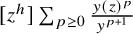 $[z^h] \sum _{p \geq 0} \frac {y(z)^p}{y^{p+1}}$
. In view of Remark 2.11, this corresponds to computing series of downward skip-free walks weighted by the
 $a_k$
and
 $b_k$
respectively – recall that these series belong to the ring
 $\mathcal {R}:=\mathbb {Q}[[t, t^\circ _1,t^\circ _2,\ldots ,t^{\bullet }_1,t_2^\bullet ,\ldots ]]$
. We discuss the enumeration of DSF walks in detail in Appendix A; let us only quote the useful results here.
Let us define an excursion as a DSF walk of any length (see again Definition 2.10) that starts at
 $0$
, ends at
 $-1$
, and always remains nonnegative in between (these objects are also called Łukasiewicz walks). We then define
 $z^\bullet (y)$
as the generating functions of excursions where, to each step with increment i, we attach a weight
 $b_i y^{-1}$
, for all
 $i \geq -1$
(recall that
 $b_{-1}=1$
). The series
 $z^\bullet (y)$
belongs to
 $\mathcal {R}[[y^{-1}]]$
, and by a standard decomposition of excursions (see Proposition A.1) we have
 $$ \begin{align} z^\bullet(y) = \sum_{k\geq -1} \frac{b_k}{y} z^\bullet(y)^{k+1} \qquad \text{i.e.} \qquad y = y(z^\bullet(y)). \end{align} $$
Remark 5.1. One may think of
 $z^\bullet (y)$
as a “compositional inverse” of
 $y(z)$
. To relate this idea to the standard notion of compositional inverse of formal power series – see, for example, [Reference Stanley55, Section 5.4] – we observe that, while
 $y(z)=z^{-1} + \sum _{k\geq 0} b_kz^{k}$
is a formal Laurent series in z, its multiplicative inverse
 $y(z)^{-1}=z+\cdots $
is a formal power (not Laurent) series without constant coefficient and with a nonzero z coefficient. As such, it indeed admits a compositional inverse in the usual sense, and this is why
 $z^\bullet (y)$
is naturally a series in
 $y^{-1}$
.
We similarly define
 $\tilde {z}^\circ (x)$
as the generating function of excursions where, to each step with increment i, we attach a weight
 $a_i x^{-1}$
, for all
 $i \geq -1$
. The series
 $\tilde {z}^\circ (x)$
belongs to
 $\mathcal {R}[[x^{-1}]]$
and satisfies
 $$ \begin{align} \tilde{z}^\circ(x) = \sum_{k\geq -1} \frac{a_k}{x} \tilde{z}^\circ(x)^{k+1} \qquad \text{i.e.} \qquad x = x\left(\tilde{z}^\circ(x)^{-1}\right). \end{align} $$
We then set
 $z^\circ (x):=\tilde {z}^\circ (x)^{-1}$
, which may be thought as the compositional inverse of
 $x(z)$
. It is a formal Laurent series in
 $x^{-1}$
, note however that its coefficients do not belong to
 $\mathcal {R}$
but to its field of fractions, as
 $\tilde {z}^\circ (x) = a_{-1} x^{-1} + \cdots $
and, by (2.9), we see that
 $a_{-1}$
has no constant coefficient so is not invertible in
 $\mathcal {R}$
. Even though we will write expressions in terms of
 $z^\circ (x)$
for symmetry reasons, in fact the reader should notice that they can be recast in terms of
 $\tilde {z}^\circ (x)$
and that, at the end, we only obtain series having their coefficients in
 $\mathcal {R}$
.
The “master” series
 $z^\bullet (y)$
and
 $z^\circ (x)$
allow to express several generating functions of weighted DSF walks. This is discussed in detail in Appendix A, where we establish the following proposition, stating the results that we need for our purposes.
Proposition 5.2. For DSF walks starting and ending at
 $0$
(“bridges”), we have
 $$ \begin{align} \begin{aligned} \sum_{p \geq 1} \frac{P^{\bullet}_{p,0}}{p y^p} &= [z^0] \sum_{p \geq 1} \frac{y(z)^p}{p y^p} = \ln \left( y \, z^\bullet(y) \right), \\ \sum_{p \geq 1} \frac{P^\circ_{p,0}}{p x^p} &= [z^0] \sum_{p \geq 1} \frac{x(z)^p}{p x^p} = \ln \left( \frac{x}{a_{-1} z^\circ(x)} \right). \end{aligned} \end{align} $$
For DSF walks starting at
 $0$
and ending at a fixed negative position
 $-h<0$
, we have
 $$ \begin{align} \begin{aligned} \sum_{p \geq 1} \frac{P^{\bullet}_{p,-h}}{p y^p} &= [z^{-h}] \sum_{p \geq 1} \frac{y(z)^p}{p y^p} = \frac{z^\bullet(y)^h}h, \\ \sum_{p \geq 1} \frac{P^\circ_{p,-h}}{p x^p} &= [z^h] \sum_{p \geq 1} \frac{x(z)^p}{p x^p} = \frac{z^\circ(x)^{-h}}{h}. \end{aligned} \end{align} $$
For DSF walks starting at
 $0$
and ending at a positive position, we have the bivariate series
 $$ \begin{align} \begin{aligned} \sum_{p \geq 1} \sum_{h \geq 1} \frac{P^{\bullet}_{p,h} u^h}{p y^p} &= \sum_{h \geq 1} u^h [z^{h}] \sum_{p \geq 1} \frac{y(z)^p}{p y^p} = \ln \left( \frac{z^\bullet(y)^{-1}-u^{-1}}{y - y(u)}\right), \\ \sum_{p \geq 1} \sum_{h \geq 1} \frac{P^\circ_{p,h} u^h}{p x^p} &= \sum_{h \geq 1} u^h [z^{-h}] \sum_{p \geq 1} \frac{x(z)^p}{p x^p} = \ln \left( a_{-1} \frac{z^\circ(x)-u^{-1}}{x-x(u^{-1})}\right). \end{aligned} \end{align} $$
Note that the right-hand sides of (5.3) belong to
 $\mathcal {R}[[y^{-1}]]$
and
 $\mathcal {R}[[x^{-1}]]$
respectively, since
 $y z^\bullet (y)$
and
 $\frac {x}{a_{-1} z^\circ (x)}$
are formal power series in
 $y^{-1}$
and
 $x^{-1}$
respectively with constant coefficient equal to
 $1$
(they count excursions with their last step removed, so
 $1$
is the contribution from the walk with
 $0$
steps). We now apply the above formulas to treat the case of pointed disks and cylinders:
Proposition 5.3. The grand generating functions of pointed disks with a monochromatic boundary read
 $$ \begin{align} \frac{\partial W^\circ(x)}{\partial t} = \frac{d}{dx} \ln z^\circ(x), \qquad \frac{\partial W^\bullet(y)}{\partial t} = - \frac{d}{dy} \ln z^\bullet(y) \end{align} $$
while those for cylinders with monochromatic boundaries read
 $$ \begin{align} \begin{aligned} W^{\circ\circ}(x_1,x_2) &= \sum_{p,q \geq 1} \frac{F^{\circ\circ}_{p,q}}{x_1^{p+1} x_2^{q+1}} = \frac{\partial^2}{\partial x_1 \partial x_2} \ln \left(\frac{z^\circ(x_1)-z^\circ(x_2)}{x_1-x_2}\right),\\ W^{\bullet\bullet}(y_1,y_2) &= \sum_{p,q \geq 1} \frac{F^{\bullet\bullet}_{p,q}}{y_1^{p+1} y_2^{q+1}} = \frac{\partial^2}{\partial y_1 \partial y_2} \ln \left(\frac{z^\bullet(y_1)-z^\bullet(y_2)}{y_1-y_2}\right),\\ W^{\circ\bullet}(x,y) &= \sum_{p,q \geq 1} \frac{F^{\circ\bullet}_{p,q}}{x^{p+1} y^{q+1}} = - \frac{\partial^2}{\partial x \partial y} \ln \left( 1 - \frac{z^\bullet(y)}{z^\circ(x)}\right). \end{aligned} \end{align} $$
Proof. We start with the case of pointed disks: we have
 $\frac {\partial W^\circ (x)}{\partial t}=\sum _{p \geq 0} \frac {\partial F_p^\circ }{\partial t} x^{-p-1} = \sum _{p \geq 0} \frac {P^\circ _{p,0}}{x^{p+1}}$
by Corollary 3.5. The latter series is obtained by acting on the second line of (5.3) with
 $-\frac {\partial }{\partial x}$
, and by adding the contribution of the
 $p=0$
term
 $\frac {P^\circ _{0,0}}x=\frac 1x$
. The case of
 $\frac {\partial W^\bullet (x)}{\partial t}$
is similar.
We now turn to the case of cylinders, for which we shall sum the expressions given in Corollary 4.2. For
 $W^{\circ \circ }(x_1,x_2)$
we may write
 $$ \begin{align} W^{\circ\circ}(x_1,x_2) & = \frac{\partial^2}{\partial x_1 \partial x_2} \sum_{p,q,h \geq 1} h \cdot \frac{[z^h]x(z)^p}{p x_1^p} \cdot \frac{[z^{-h}]x(z)^q}{q x_2^q} \nonumber \\ &\overset{(5.4)}{=} \frac{\partial^2}{\partial x_1 \partial x_2} \sum_{q,h\geq 1} z^\circ(x_1)^{-h} \cdot \frac{[z^{-h}]x(z)^q}{q x_2^q} \overset{(5.5)}{=} \frac{\partial^2}{\partial x_1 \partial x_2} \ln \left( a_{-1} \frac{z^\circ(x_2)-z^\circ(x_1)}{x_2-x(z^\circ(x_1))}\right) \end{align} $$
which yields the first line of (5.7) using
 $x(z^\circ (x_1))=x_1$
(the
 $a_{-1}$
factor can be removed due to the differentiation). The case of
 $W^{\bullet \bullet }(y_1,y_2)$
is similar. Finally, for
 $W^{\circ \bullet }(x,y)$
we may write
 $$ \begin{align} W^{\circ\bullet}(x,y) = \frac{\partial^2}{\partial x \partial y} \sum_{p,q,h \geq 1} h \cdot \frac{[z^h]x(z)^p}{p x^p} \cdot \frac{[z^{-h}]y(z)^q}{q y^q} \overset{(5.4)}{=} \frac{\partial^2}{\partial x \partial y} \sum_{h \geq 1} \frac{1}h \left(\frac{z^\bullet(y)}{z^\circ(x)}\right)^h \end{align} $$
which yields the last line of (5.7).
Note that it does not seem possible to compute by the above method the grand generating function associated with
 $\tilde {F}^{\bullet \circ }_{p,q}$
. We will consider another method, under the assumption of bounded face degrees, in Section 5.3.
5.2 Monochromatic disks and the spectral curve
We now treat the case of monochromatic disks in the following:
Proposition 5.4. The grand generating functions
 $W^{\circ }(x)$
and
 $W^{\bullet }(y)$
of disks with monochromatic boundaries are given by
 $$ \begin{align} W^\circ(x) = y(z^\circ(x)) - \sum_{d \geq 1} t^\circ_d x^{d-1}, \qquad W^\bullet(y) = x(z^\bullet(y)) - \sum_{d \geq 1} t^{\bullet}_d y^{d-1}. \end{align} $$
Under the assumption of bounded face degrees (
 $t^\circ _d=t^{\bullet }_d=0$
for d large enough), these identities hold within
 $\mathcal {R}((x^{-1}))$
and
 $\mathcal {R}((y^{-1}))$
respectively. Without this assumption, they hold within the respective larger rings
 $\mathbb {Q}((x^{-1}))[[t, t^\circ _1,t^\circ _2,\ldots ,t^{\bullet }_1,t_2^\bullet ,\ldots ]]$
and
 $\mathbb {Q}((y^{-1}))[[t, t^\circ _1,t^\circ _2,\ldots ,t^{\bullet }_1,t_2^\bullet ,\ldots ]]$
, in which the substitutions
 $y(z^\circ (x))$
and
 $x(z^\bullet (y))$
are respectively well-defined.
Proof. Let us prove the first identity, the argument for the second being entirely similar. For simplicity, let us first present the idea of the computation, without paying attention to the ring in which we are working. On the one hand, we may write
 $$ \begin{align} y(z^\circ(x)) = z^\circ(x)^{-1} + \sum_{k \geq 0} b_k z^\circ(x)^{k} \overset{({2.8})}{=} z^\circ(x)^{-1} + \sum_{d \geq 1} t_d^\circ \sum_{k \geq 0} z^\circ(x)^{k} [z^{k}] x(z)^{d-1}. \end{align} $$
On the other hand, by (4.6), we have
 $$ \begin{align} W^\circ(x) = \sum_{p\geq 0}\frac{F_p^\circ}{x^{p+1}} = \sum_{p\geq 0} \frac{[z]x(z)^{p+1}}{(p+1)x^{p+1}} - \sum_{p\geq 0} \sum_{d \geq 2} t_d^\circ \sum_{h \geq 1} h \frac{[z^h]x(z)^{p+1}}{(p+1)x^{p+1}} [z^{-h}] x(z)^{d-1}. \end{align} $$
By (5.4), we deduce
 $$ \begin{align} W^\circ(x) = z^\circ(x)^{-1} - \sum_{d \geq 2} t_d^\circ \sum_{h \geq 1} z^\circ(x)^{-h} [z^{-h}] x(z)^{d-1}. \end{align} $$
By doing a change of variable
 $k=-h$
in the right-hand side, the sum can be combined with that in the right-hand side of (5.11) to yield
 $$ \begin{align} y(z^\circ(x)) - W^\circ(x) = \sum_{d \geq 1} t_d^\circ \sum_{k \in \mathbb{Z}} z^\circ(x)^{k} [z^{k}] x(z)^{d-1} = \sum_{d \geq 1} t_d^\circ \,x \left(z^\circ(x)\right)^{d-1} = \sum_{d \geq 1} t_d^\circ x^{d-1}, \end{align} $$
which gives the wanted identity.
Let us now discuss in which ring the above computations make sense. Introducing the shorthand notations
 $$ \begin{align} \begin{aligned} \mathcal{R}_1 &:= \mathcal{R}((x^{-1})) = \mathbb{Q}[[t, t^\circ_1,t^\circ_2,\ldots,t^{\bullet}_1,t_2^\bullet,\ldots]]((x^{-1})) \\ \mathcal{R}_2 &:= \mathbb{Q}((x^{-1}))[[t, t^\circ_1,t^\circ_2,\ldots,t^{\bullet}_1,t_2^\bullet,\ldots]] \end{aligned} \end{align} $$
observe that we have the strict inclusion
 $$ \begin{align} \mathcal{R}_1 \subsetneq \mathcal{R}_2. \end{align} $$
The series
 $W^{\circ }(x)$
belongs to
 $\mathcal {R}_1$
hence to
 $\mathcal {R}_2$
, however we have
 $\sum _{d \geq 1} t^\circ _d x^{d-1} \in \mathcal {R}_2 \setminus \mathcal {R}_1$
unless we make the assumption of bounded degrees. Let us check that, in full generality, the substitution
 $y(z^\circ (x))$
makes sense within
 $\mathcal {R}_2$
: for this we return to (5.11) and note that, in the right-hand side, the quantity
 $[z^{k}] x(z)^{d-1}$
vanishes if
 $k \geq d$
, and is of the form
 $(a_{-1})^k C_{d,k}$
for some
 $C_{d,k} \in \mathcal {R}$
if
 $0 \leq k \leq d-1$
(as
 $x(z)=a_{-1} z + \cdots $
). Thus, we have
 $$ \begin{align} y(z^\circ(x)) = z^\circ(x)^{-1} + \sum_{d \geq 1} t_d^\circ \sum_{k=0}^{d-1} C_{d,k} \left(a_{-1} z^\circ(x)\right)^k. \end{align} $$
Now, we observe that
 $a_{-1} z^\circ (x)$
belongs to
 $\mathcal {R}_1$
, since it is the multiplicative inverse of
 $\tilde {z}^\circ (x)/a_{-1}=x^{-1}+ \cdots \in \mathcal {R}[[x^{-1}]]$
, so that
 $a_{-1}z^\circ (x)=x(1+S(x))$
, where
 $S(x)\in \mathcal {R}[[x^{-1}]]$
. Hence,
 $\sum _{k=0}^{d-1} C_{d,k} \left (a_{-1} z^\circ (x)\right )^k $
also belongs to
 $\mathcal {R}_1$
for any
 $d \geq 1$
. Under the assumption of bounded face degrees, this shows that
 $y(z^\circ (x))$
is a well-defined element of
 $\mathcal {R}_1$
as wanted. Without this assumption, consider an arbitrary (finite) monomial T in
 $t, t^\circ _1,t^\circ _2,\ldots ,t^{\bullet }_1,t_2^\bullet ,\ldots $
, then for d large enough
 $t_d^\circ $
does not appear in T, and hence only finitely many terms in the right-hand side of (5.17) contribute to the coefficient of T. This means that
 $y(z^\circ (x))$
is a well-defined element of
 $\mathcal {R}_2$
, as wanted.
Remark 5.5. For bookkeeping purposes, let us write down the black analogue of (5.13):
 $$ \begin{align} W^{\bullet}(x) = a_{-1} z^{\bullet}(x) - \sum_{d \geq 2} t_{d}^{\bullet} \sum_{h \geq 1} z^{\bullet}(x)^{h} [z^{h}] y(z)^{d-1}. \end{align} $$
Remark 5.6. Our discussion of the rings in which the identities (5.10) hold is somewhat inspired from [Reference Gessel44, Section 2]. This reference considers the ring
 $\mathbb {C}((T))[[Y]]$
of formal power series in a variable Y whose coefficients are formal Laurent series in another variable T (we capitalize the letters to avoid confusions with the notations of the present paper). Here, we are replacing T by
 $x^{-1}$
or
 $y^{-1}$
, and Y by a collection of variables
 $t,t_1^\circ ,\ldots$
, which does not change fundamentally the discussion.
For simplicity, let us now make the assumption of bounded face degrees, in which case Lemma 2.7 asserts that
 $x(z)$
and
 $y(z)$
are Laurent polynomials. They define the so-called spectral curve, see [Reference Eynard40, Definition 8.3.1]. Then, interestingly, Proposition 5.4 may be reformulated in the following form, which corresponds essentially to [Reference Eynard40, Theorem 8.3.1]Footnote
10
.
Proposition 5.7 (Rational parametrization of disk generating functions)
Consider the series
 $$ \begin{align} Y(x) := W^\circ(x) + \sum_{d=1}^{\Delta^{\!\circ}} t^\circ_d x^{d-1}, \qquad X(y) := W^\bullet(y) + \sum_{d=1}^{\Delta^{\!\bullet}} t^{\bullet}_d y^{d-1} \end{align} $$
where
 $\Delta ^{\!\circ },\Delta ^{\!\bullet }$
are the maximal degrees for white and black faces, respectively. Then, we have the rational parametrization
 $$ \begin{align} Y(x(z))=y(z), \qquad X(y(z))=x(z). \end{align} $$
Proof. Proposition 5.4 asserts that
 $Y(x)=y(z^\circ (x))$
and
 $X(y)=x(z^\bullet (y))$
. As discussed in Section 5.1,
 $z^\circ (x)$
and
 $z^\bullet (y)$
can be seen as compositional inverses of
 $x(z)$
and
 $y(z)$
respectively. Therefore, we get the wanted relations (5.20) by substituting
 $x=x(z)$
into
 $Y(x)$
and
 $y=y(z)$
into
 $X(y)$
. Note that these operations are well-defined since
 $Y(x)$
is here a formal Laurent series in
 $x^{-1}$
, which we substitute by
 $x(z)^{-1}$
which is a formal power series in
 $z^{-1}$
without constant coefficient, and similarly for the other relation.
5.3 Disks with a Dobrushin boundary condition and the resultant
In this section we make the assumption of bounded face degrees (
 $t^\circ _d=t^{\bullet }_d=0$
for d large enough) so that, by Lemma 2.7,
 $x(z)$
and
 $y(z)$
are Laurent polynomials. Our purpose is to show that the expression obtained in Proposition 4.5 for the generating function of hypermaps with a Dobrushin boundary is consistent with the expressions given in [Reference Eynard40]. We first state the following complement to Proposition 5.2 on the enumeration of weighted DSF walks. It is also established in Appendix A.
Proposition 5.8. Let
 $\Delta ^{\!\circ }$
be a fixed positive integer and set
 $t_k^\circ =0$
for
 $k>\Delta ^{\!\circ }$
. Then, over the field of Puiseux series in
 $y^{-1}$
, the algebraic equation
 $y(z)=y$
admits
 $\Delta ^{\!\circ }$
solutions. One of them is the generating function of excursions
 $z^\bullet (y)$
defined above. Denoting the other ones by
 $z_1^\bullet (y),\ldots ,z_{\Delta ^{\!\circ }-1}^\bullet (y)$
, we have for any
 $h>0$
 $$ \begin{align} \sum_{p \geq 1} \frac{P^{\bullet}_{p,h}}{p y^p} = [z^{h}] \sum_{p \geq 1} \frac{y(z)^p}{p y^p} = \sum_{i=1}^{\Delta^{\!\circ}-1} \frac{z_i^\bullet(y)^{-h}}h. \end{align} $$
Similarly, let
 $\Delta ^{\!\bullet }$
be a fixed positive integer and set
 $t_k^\bullet =0$
for
 $k>\Delta ^{\!\bullet }$
. Then, over the field of Puiseux series in
 $x^{-1}$
, the algebraic equation
 $x(z)=x$
admits
 $\Delta ^{\!\bullet }$
solutions. One of them is the inverse
 $z^\circ (x)$
of the generating function of excursions defined above. Denoting the other ones by
 $z_1^\circ (y),\ldots ,z_{\Delta ^{\!\bullet }-1}^\circ (y)$
, we have for any
 $h>0$
 $$ \begin{align} \sum_{p \geq 1} \frac{P^\circ_{p,h}}{p x^p} = [z^{-h}] \sum_{p \geq 1} \frac{x(z)^p}{p x^p} = \sum_{i=1}^{\Delta^{\!\bullet}-1} \frac{z_i^\circ(y)^{h}}h. \end{align} $$
Note that these expressions correspond to the coefficients of
 $u^h$
in the two series (5.5). From them we get an interesting expression for the grand generating function of disks with a Dobrushin boundary condition.
Proposition 5.9. Under the assumption of bounded face degrees, we have

Proof. Rewrite the left-hand side using the second line of (4.7). Evaluate the sums over
 $p,q$
using (5.4) for
 $h>0$
, and Proposition 5.8 for
 $h<0$
. The sum over
 $h>0$
is then equal to
 $-\ln \left ( 1 - \frac {z^\bullet (y)}{z^\circ (x)}\right )$
, and the sum over
 $h<0$
to
 $\sum _{i=1}^{\Delta ^{\!\bullet }-1} \sum _{j=1}^{\Delta ^{\!\circ }-1} \ln \left ( 1 - \frac {z_i^\circ (x)}{z_j^\bullet (y)}\right )$
. Taking the exponential, the wanted expression follows.
In the remainder of this section, we will argue that this expression is equivalent to that given in [Reference Eynard40]. Let us consider the resultant
 $r(x,y)$
of the two following polynomials in z:
 $$ \begin{align} z^{\Delta^{\!\bullet}-1}(x(z)-x) = \sum_{k=-1}^{\Delta^{\!\bullet}-1} (a_k - x \delta_{k,0}) z^{\Delta^{\!\bullet}-1-k}, \qquad z (y(z)-y) = \sum_{k=-1}^{\Delta^{\!\circ}-1} (b_k - y \delta_{k,0}) z^{k+1}. \end{align} $$
On the one hand, the resultant is by definition the determinant
 $$ \begin{align} r(x,y) := \det\, \begin{pmatrix} a_{-1} & a_0 -x & a_1 & \cdots & a_{\Delta^{\!\bullet}-1} & & &\\ & a_{-1} & a_0 -x & a_1 & \cdots & a_{\Delta^{\!\bullet}-1} & &\\ & & \ddots & \ddots & \ddots & \ddots & \ddots &\\ & & & a_{-1} & a_0 -x & a_1 & \cdots & a_{\Delta^{\!\bullet}-1} \\ b_{\Delta^{\!\circ} -1 } & \cdots & b_1 & b_0 - y & 1 & & &\\ & b_{\Delta^{\!\circ} -1 } & \cdots & b_1 & b_0 - y & 1 & & \\ & & \ddots & \ddots & \ddots & \ddots & \ddots &\\ & & & b_{\Delta^{\!\circ} -1 } & \cdots & b_1 & b_0 - y & 1 \\ \end{pmatrix} \end{align} $$
where the undisplayed entries are equal to
 $0$
. This quantity is proportional to
 $E(x,y)$
as given in [Reference Eynard40, Theorem 8.3.2, p. 378], up to the change of notation given in (2.11).
On the other hand, the resultant can be expressed in terms of the roots of the polynomials. Namely, using the factorizations
 $$ \begin{align} z^{\Delta^{\!\bullet}-1}(x(z)-x)= a_{-1} \prod_{i=0}^{\Delta^{\!\bullet}-1} (z-z_i^\circ(x)), \qquad z (y(z)-z) = b_{\Delta^{\!\circ}-1} \prod_{j=0}^{\Delta^{\!\circ}-1} (z-z_j^\bullet(y)), \end{align} $$
where we denote by
 $z_0^\circ (x)=z^\circ (x)$
and
 $z_0^\bullet (y)=z^\bullet (y)$
the “zeroth” roots, we find
 $$ \begin{align} \begin{aligned} r(x,y) &= (a_{-1})^{\Delta^{\!\circ}} (b_{\Delta^{\!\circ}-1})^{\Delta^{\!\bullet}} \prod_{i=0}^{\Delta^{\!\bullet}-1} \prod_{j=0}^{\Delta^{\!\circ}-1} \left( z_i^\circ(x) - z_j^\bullet(y) \right) \\ &= (a_{-1})^{\Delta^{\!\circ}} \prod_{i=0}^{\Delta^{\!\bullet}-1} \prod_{j=0}^{\Delta^{\!\circ}-1} \left( 1 - \frac{z_i^\circ(x)}{z_j^\bullet(y)}\right) \end{aligned} \end{align} $$
where we use the fact that
 $b_{\Delta ^{\!\circ }-1} \prod _{j=0}^{\Delta ^{\!\circ }-1} (-z_j^\bullet (y))=b_{-1}=1$
since it corresponds to the constant coefficient of the polynomial
 $z(y(z)-z)$
. The above double product is very close to that in Proposition 5.9, but it involves the extra zeroth roots. To make the two expressions match, we shall divide the above display by the two relations (5.26) taken at
 $z=z_0^\bullet (y)$
and
 $z=z_0^\circ (x)$
respectively. This yields

where
 $X(y)=x(z_0^\bullet (y))$
and
 $Y(x)=y(z_0^\circ (y))$
are as in Proposition 5.7. By substituting
 $x=x(z)$
and
 $y=y(z')$
we recover, up to notations, the expression given at [Reference Eynard40, Equation (8.4.6), p. 397] for
 $c=-1$
.
6 Conclusion
In this paper, we have shown how to enumerate bijectively a number of families of planar hypermaps using the slice decomposition. We thus recovered several of the intriguing formulas given in [Reference Eynard40, Chapter 8]. In particular, we have seen that the fact that generating functions for hypermaps admit rational parametrizations is closely related with the enumeration of downward skip-free walks: the parameter in which the series are rational can be interpreted as the generating function of excursions.
Another novelty of our approach is the introduction of trumpets and cornets, that is hypermaps with two boundaries, one of them tight. Such families of hypermaps have not been considered previously, but turn out to be important building blocks to which other families of hypermaps can be reduced. Trumpets and cornets also appear as natural objects in the blossoming tree approach of the forthcoming paper [Reference Albenque, Ménard and Tokka4].
In contrast with the case of ordinary, nonbicolored maps, the slice decomposition for hypermaps relies heavily on the canonical orientation of the edges, and leads to considerations specific to the world of directed graphs. In particular, our approach to enumerate planar hypermaps with Dobrushin boundaries hinges on a decomposition into strongly connected components. This idea can be generalized to handle arbitrary boundary conditions; this is the subject of two papers in preparation [Reference Bouttier, Eynard and Lejeune25, Reference Lejeune51].
A Generating functions of downward skip-free walks
The purpose of this appendix is to review some enumeration results about downward skip-free walks, which we need in this paper. Precisely, we shall establish Propositions 5.2 and 5.8. Since the discussion is more about walks than hypermaps, we state the results using independent notation, and it is only at the end that we make the connection with the conventions and notation of the main text. Let us mention that the enumeration of one-dimensional walks, sometimes also called directed lattice paths, is a very classical topic, see for instance [Reference Banderier and Flajolet5, Reference Banderier, Lackner and Wallner6] and references thereinFootnote 11 . Note that our terminology differs slightly from these references. An originality of our discussion is that it specifically focuses on downward skip-free walks.
Recall from Definition 2.10 that a downward skip-free walk, or DSF walk for short, is a finite sequence of integers
 $(\pi _0,\pi _1,\ldots ,\pi _\ell )$
of arbitrary length, such that at each step
 $i=1,\ldots ,\ell $
, the increment
 $\pi _i-\pi _{i-1}$
is greater than or equal to
 $-1$
. The integers
 $\pi _0,\pi _1,\ldots ,\pi _\ell $
are called the positions of the walk, with
 $\pi _0$
the starting position and
 $\pi _\ell $
the final position. Given formal variables
 $p_{-1},p_0,p_1,p_2,\ldots $
, we attach a weight
 $p_j$
to each step with increment j, for each
 $j=-1,0,1,2,\ldots $
. We then define the weight of a DSF walk as the product of its step weights.
A first simple observation is that, introducing the formal Laurent series
 $$ \begin{align} P(u) := p_{-1} u^{-1} + p_0 + p_1 u + p_2 u^2 + \cdots, \end{align} $$
the quantity
 $P(u)^\ell $
may be expanded as a sum over all DSF walks with
 $\ell $
steps starting at position
 $\pi _0=0$
, the exponent of u recording the final position
 $\pi _\ell $
. Thus, the coefficient
 $$ \begin{align} P_{\ell,h} := [u^h] P(u)^\ell \end{align} $$
is the sum of weights of all DSF walks with
 $\ell $
steps, starting at
 $0$
and ending at h. Clearly,
 $P_{\ell ,h}$
is an element of the ring
 $\mathcal {P}:=\mathbb {Q}[p_{-1},p_0,p_1,p_2,\ldots ]$
of polynomials in the
 $p_j$
with rational coefficients.
Next, we consider excursions, namely DSF walks which start at
 $0$
, end at
 $-1$
, and always remain nonnegative in between (these objects are also called Łukasiewicz walks). We denote by
 $U(s)$
the generating function of excursions with an arbitrary number of steps, where we incorporate an extra auxiliary weight s per step. It is an element of the ring
 $\mathcal {P}[[s]]$
of formal power series in s with coefficients in
 $\mathcal {P}$
. We then have:
Proposition A.1. The generating function
 $U(s)$
of excursions is the unique series in
 $\mathcal {P}[[s]]$
satisfying
 $$ \begin{align} 1 = s P(U(s)) \end{align} $$
or equivalently
 $$ \begin{align} U(s) = s \left( p_{-1} + p_0 U(s) + p_1 U(s)^2 + p_2 U(s)^3 + \cdots \right). \end{align} $$
This follows from a classical “last-passage” decomposition: given an excursion, denote by j the increment of its first step. Then, consider the last passages of the walk by the positions
 $j-1, j-2,\ldots ,1,0,-1$
(such passages necessarily exist since the walk is downward skip-free): this yields a decomposition of the excursion into its first step followed by the concatenation of
 $j+1$
(suitably shifted) excursions. Thus, the generating function of excursions starting with a step of increment j is equal to
 $s p_j U(s)^{j+1}$
, and we obtain (A.4) by summing over j.
A similar last-passage decomposition implies that, for any
 $k \geq 1$
, the series
 $U(s)^k$
is equal to the generating function of DSF walks which start at
 $0$
, end at
 $-k$
, and remain strictly above
 $-k$
before. The classical cycle lemma – see, for example, [Reference Stanley55, Chapter 5] or [Reference Flajolet and Sedgewick43, ⊳ I.47] and references therein – asserts that
 $$ \begin{align} [s^\ell] U(s)^k = \frac{k}{\ell} P_{\ell,-k}, \qquad k,\ell \geq 1. \end{align} $$
In other words, out of all DSF walks with
 $\ell $
steps starting at
 $0$
and ending at
 $-k$
, a fraction
 $k/\ell $
remain strictly above
 $-k$
until the last step. The cycle lemma may be rewritten as
 $$ \begin{align} \sum_{\ell \geq 0} P_{\ell,-k} s^\ell = s U(s)^{k-1} U'(s), \qquad k \geq 1. \end{align} $$
This expression remains in fact valid for
 $k=0$
. Indeed, observe that a general DSF walk from
 $0$
to
 $-1$
can be uniquely decomposed as the concatenation of an excursion and of a general walk from
 $-1$
to
 $-1$
, which by shifting the latter gives the relation
 $s U'(s) = U(s) \sum _{\ell \geq 0} P_{\ell ,0} s^\ell $
.
We would like to find a counterpart of (A.6) for DSF walks starting at
 $0$
and ending at a positive position. To this end, let us define, for all
 $h \geq 0$
, an arch of tilt h as a DSF walk which starts at
 $0$
, ends at h, and remains at positions
 $\geq h$
in between. An arch of tilt h is said strict if it has at least one step and remains at positions
 $>h$
in between its starting and ending positions. Let us denote by
 $A_h^\geq (s)$
and
 $A_h^>(s)$
the generating functions of arches and strict arches of tilt h, respectively. Let us make the observation that
 $$ \begin{align} A_0^\geq(s) = \frac{1}{1-A_0^>(s)} \end{align} $$
since an arch of tilt
 $0$
is the concatenation of an arbitrary number of strict arches of tilt
 $0$
. Furthermore, we have
 $$ \begin{align} A_h^\geq(s)=A_h^>(s) A_0^\geq(s) =\frac{A_h^>(s)}{1-A_0^>(s)} \qquad \text{for } h>0 \end{align} $$
since an arch of tilt h is the concatenation of a strict arch of the same tilt, and of a (suitably shifted) arch of tilt
 $0$
. Finally, we have
 $$ \begin{align} A_h^>(s) = s \sum_{j \geq h} p_j U(s)^{j-h} \qquad \text{for } h\geq 0 \end{align} $$
as seen by decomposing a strict arch according to the increment j of its first step. All these relations allow to express the
 $A_h^\geq (s)$
and
 $A_h^>(s)$
in terms of the “master” series
 $U(s)$
. But notice that we also have
 $$ \begin{align} U(s) = s p_{-1} A_0^\geq(s) = \frac{s p_{-1}}{1-A_0^>(s)} \end{align} $$
since an excursion is obtained by appending a final downward step to an arch of tilt
 $0$
. Combining with (A.9) at
 $h=0$
, we recover the relation (4) determining
 $U(s)$
. All the above combinatorial relations may be conveniently encoded into the following:
Proposition A.2 (formal Wiener-Hopf factorization)
Within the ring
 $\mathcal {P}((u))[[s]]$
of formal power series in s whose coefficients are themselves formal Laurent series in u with coefficients in
 $\mathcal {P}$
, we have
 $$ \begin{align} \begin{aligned} 1 - s P(u) &= \left( 1 - \frac{U(s)}u \right) \left( 1 - \sum_{h \geq 0} A_h^>(s) u^h \right) \\ &= \frac{sp_{-1}}{U(s)} \left( 1 - \frac{U(s)}u \right) \left( 1 - \sum_{h > 0} A_h^\geq(s) u^h \right). \end{aligned} \end{align} $$
or equivalently
 $$ \begin{align} \begin{aligned} \frac1{1 - s P(u)} &= \frac1{1 - \frac{U(s)}u} \cdot \frac1{1 - \sum_{h \geq 0} A_h^>(s) u^h} \\ &= \frac{U(s)}{sp_{-1}} \cdot \frac1{1 - \frac{U(s)}u} \cdot \frac1{1 - \sum_{h > 0} A_h^\geq(s) u^h}. \end{aligned} \end{align} $$
Proof. We establish the first equality in (A.11) by checking that the coefficients of
 $u^h$
on both sides are equal for any
 $h \in \mathbb {Z}$
:
-
○ for
$h<-1$
they simply vanish, -
○ for
$h=-1$
we find the identity
$-s p_{-1} = - U(s) (1-A^>_0(s))$
equivalent to (A.10), -
○ for
$h\geq 0$
we find the identity
$-s p_h=-A_h^>(s)+U(s) A_{h+1}^>(s)$
resulting from (A.9).


We then pass to the second line of (A.11) using (A.8) and (A.10) again. We then obtain (A.12) by inverting within
 $\mathcal {P}((u))[[s]]$
.
Remark A.3. There is also a bijective proof of (A.12), which consists in decomposing a general DSF walk into a sequence of excursions followed by a sequence of arches (which may be taken strict or not, hence the two versions of the identity). Let us not enter into details here, but refer instead to the closely related discussion in [Reference Banderier, Lackner and Wallner6].
For our purposes it is convenient to take the logarithm of (A.12), which gives the relation
 $$ \begin{align} \sum_{\ell \geq 1} \frac{s^\ell P(u)^\ell}\ell = \ln \frac{U(s)}{s p_{-1}} + \sum_{k \geq 1} \frac{U(s)^k}{k u^k} + \ln \frac1{1 - \sum_{h> 0} A_h^\geq(s) u^h}. \end{align} $$
Notice that, in the right-hand side, the first term does not contain the variable u, while the second and third terms contain only negative and positive powers of u respectively. Extracting the nonpositive powers of u in the relation, we get the identities
 $$ \begin{align} \sum_{\ell \geq 1} \frac{P_{\ell,0} s^\ell}\ell = \ln \frac{U(s)}{s p_{-1}}, \qquad \qquad \sum_{\ell \geq 1} \frac{P_{\ell,-h} s^\ell}\ell = \frac{U(s)^h}h \qquad \text{for } h>0 \end{align} $$
which amount again to the cycle lemma. For positive powers of u, there is a priori no such simple identities, but we may write
 $$ \begin{align} \sum_{h \geq 1} \sum_{\ell \geq 1} \frac{P_{\ell,h} s^\ell u^h}{\ell} = \ln \frac1{1 - \sum_{h> 0} A_h^\geq(s) u^h} = \ln \left( p_{-1} \frac{U(s)^{-1}-u^{-1}}{1-sP(u)} \right). \end{align} $$
It is possibly to get a bit further by imposing a global bound on increments, that is by fixing a positive integer d and setting
 $p_j=0$
for
 $j>d$
. In that case,
 $P(u)=p_{-1} u^{-1}+\cdots +p_d u^d$
is a Laurent polynomial in u, and the equation
 $1=sP(u)$
admits
 $d+1$
roots in a suitable completion of
 $\mathcal {P}[[s]]$
. One of these roots is the generating function of excursions
 $U(s)$
. The other roots may be constructed as follows: consider the formal power series in V
 $$ \begin{align} \sigma(V) := V \left( 1+ \frac{p_{d-1}}{p_d} V + \cdots + \frac{p_{-1}}{p_d} V^{d+1} \right)^{-1/d} \end{align} $$
where we expand
 $(1+\cdots )^{-1/d}$
in the standard way. The constant coefficient vanishes and the coefficient of V is
 $1$
, hence
 $\sigma (V)$
admits a compositional inverse which we denote by
 $V(\sigma )$
. Then, denoting by
 $\omega _1,\ldots ,\omega _d$
the d-th roots of unity, for each
 $i=1,\ldots ,d$
, we set
 $U_i(s):=V(\omega _i (p_d s)^{1/d})^{-1}$
to be the Puiseux series in s obtained by substituting
 $\sigma =\omega _i (p_d s)^{1/d}$
in
 $V(\sigma )$
, and taking the multiplicative inverse. It is straightforward to check that it satisfies
 $1=sP(U_i(s))$
. Note that the leading term in
 $U_i(s)$
is
 $\omega _i^{-1} (p_d s)^{-1/d}$
, involving a negative exponent of s. For this reason,
 $U_1(s),\ldots ,U_d(s)$
are called the large roots of the equation
 $1=sP(u)$
, while
 $U_0(s):=U(s)$
is called the small root as it only contains positive powers of s. With all these roots at hand, we may split the Laurent polynomial
 $1-sP(u)$
as
 $$ \begin{align} 1-sP(u) = - \frac{p_d s}{u} \prod_{i=0}^d (u-U_i(s)) = \frac{p_{-1} s}{U(s)} \left( 1 - \frac{U(s)}{u} \right) \prod_{i=1}^d \left( 1 - \frac{u}{U_i(s)} \right). \end{align} $$
Here, the second equality is obtained by noting that the product of all roots (large and small) is equal to
 $(-1)^{d+1}p_{-1}/p_d$
. Comparing with (A.11), we deduce that
 $$ \begin{align} 1 - \sum_{h> 0} A_h^\geq(s) u^h = \prod_{i=1}^d \left( 1 - \frac{u}{U_i(s)} \right) \end{align} $$
and, by (A.15), we get
 $$ \begin{align} \sum_{\ell \geq 1} \frac{P_{\ell,h} s^\ell}\ell = \sum_{i=1}^d \frac{U_i(s)^{-h}}h \qquad \text{for }h>0. \end{align} $$
This is the last identity that we need for our purposes:
Proof of Propositions 5.2 and 5.8
The identities involving
 $P^{\bullet }_{p,\ldots }$
are obtained by substituting
 $p_j=b_j$
,
 $u=y^{-1}$
,
 $U(s)=z^\bullet (y)$
,
 $d=\Delta ^{\!\circ }-1$
and
 $U_i(s)=z_i^\bullet (y)$
in (A.14), (A.15) and (A.19) (recall that
 $b_{-1}=1$
). Similarly, for the identities involving
 $P^\circ _{p,\ldots }$
we substitute
 $p_j=a_j$
,
 $u=x^{-1}$
,
 $U(s)=\tilde {z}^\circ (y)=z^\circ (x)^{-1}$
,
 $d=\Delta ^{\!\bullet }-1$
,
 $U_i(s)=z_i^\circ (x)^{-1}$
.
Let us conclude this appendix by mentioning that, in [Reference Banderier and Flajolet5, Reference Banderier, Lackner and Wallner6], the equation
 $1-sP(u)$
is called the kernel equation, and that its roots play a fundamental role. These references consider one-dimensional walks which are not necessarily downward-skip free, but still have a global bound on their increments, in the sense that in addition to the upper bound d on positive increments there exists another positive integer c such that
 $p_j=0$
for
 $j<-c$
. Downward skip-free walks correspond to the particular case
 $c=1$
. In general, the kernel equation admits c small roots and d large roots. The take home message from [Reference Banderier and Flajolet5, Reference Banderier, Lackner and Wallner6] is that the generating functions of several families of constrained walks (the so-called bridges, excursions, meanders…) can be expressed as symmetric polynomials of the small roots, or of the inverses of the large roots, as we may observe here on a specific instance in (A.19).
B An alternative approach to the enumeration of monochromatic disks
In this appendix we derive an expression for the disk generating functions
 $F_p^\circ $
and
 $F_p^\bullet $
by building on some ideas introduced in [Reference Bouttier and Guitter22, Section 3.3] and extending them to the setting of hypermaps. Let us mention that the intermediate case of so-called constellations was treated in [Reference Albenque and Bouttier1]. This provides an alternative proof to the approach of Section 4.2.
Following the above references, we make a detour via a subfamily of pointed disks. Namely, we consider pointed disks with a monochromatic boundary condition, and the extra constraint that, among all vertices incident to the boundary face, the directed distance to the pointed vertex attains a minimum at the vertex incident to the root corner. By Definition 3.6, this says that the label boundary condition has a minimum at the root vertex and, following the terminology of Appendix A, that it forms an arch of tilt
 $0$
.
Let us denote by
 $F_p{}^{{\tiny \circ ,\!\geq }}$
and
 $F_p{}^{{\tiny {\bullet },\!\geq }}$
the generating function of such hypermaps with respectively a white and a black boundary of degree p. For any
 $h \geq 0$
, let us furthermore denote by
 $P_{p,-h}^{{\tiny \circ ,\!\geq }}$
(resp.
 $P_{p,-h}^{{\tiny {\bullet },\!\geq }}$
) the generating function of DSF walks with p steps starting at
 $0$
and ending at
 $-h$
, that not visit positions smaller than
 $-h$
, and carry a weight
 $a_k$
(resp.
 $b_k$
) per step of increment k. We first take
 $h=0$
in the following lemma, which is an immediate consequence of Proposition 3.7.
Lemma B.1. For any
 $p \geq 0$
, we have
 $$ \begin{align} F_p^{{\tiny \circ,\!\geq}} = t P_{p,0}^{{\tiny \circ,\!\geq}} \qquad \text{and} \qquad F_p^{{\tiny \circ,\!\geq}} = t P_{p,0}^{{\tiny \circ,\!\geq}}, \end{align} $$
where the factor t accounts for the pointed vertex.
Now, let us observe that unpointed disks can be seen as pointed disks in which the pointed vertex
 $v^\star $
coincides with the root vertex
 ${\text {v}}(\rho )$
. It is clear from Definition 3.6 that, for such pointed disks, the label boundary condition is a DSF walk never visiting negative positions. Thus, all hypermaps contributing to
 $F_p^\circ $
(resp.
 $F_p^\bullet $
) also contribute to
 $F_p^{{\tiny \circ ,\!\geq }}$
(resp.
 $F_p^{{\tiny \bullet ,\!\geq }}$
). The remaining contribution comes from the pointed disks such that the pointed vertex
 $v^\star $
differs from the root vertex
 ${\text {v}}(\rho )$
. We denote by
 $F_p^{{\tiny \circ ,\!>}}$
and
 $F_p^{{\tiny \bullet ,\!>}}$
the generating function of such hypermaps with respectively a white or a black boundary of degree p. By the above discussion we have
 $$ \begin{align} F_p^\circ = F_p^{{\tiny \circ,\!\geq}} - F_p^{{\tiny \circ,\!>}} \qquad \text{and} \qquad F_p^\bullet = F_p^{{\tiny \bullet,\!\geq}} - F_p^{{\tiny \bullet,\!>}}. \end{align} $$
The interest of these seemingly tautological equalities lies in the following:
Lemma B.2. For any
 $p \geq 0$
we have
 $$ \begin{align} F_p^{{\tiny \circ,\!>}}= a_{-1}\sum_{d \geq 2} t_d^\circ \sum_{h\geq 1}P^\circ_{d-1,h+1}P^{{\tiny \circ,\!\geq}}_{p,-h} \quad \text{and} \quad F_p^{{\tiny \bullet,\!>}}= \sum_{d\geq 2} t_{d}^{\bullet} \sum_{h\geq 1}P^{\bullet}_{d-1,h+1}P^{{\tiny \bullet,\!\geq}}_{p,-h} \end{align} $$
where
 $P^\circ _{\cdot ,\cdot }$
and
 $P^{\bullet }_{\cdot ,\cdot }$
are as in (2.7).
Proof. Note first that, for
 $p=0$
, both relations hold since everything vanishes. Let us prove the first relation for
 $p \geq 1$
, the other is just obtained by exchanging the colors (recall that
 $b_{-1}=1$
). Let
 $(\text {m},v^*)$
be a pointed disk contributing to
 $F_p^{{\tiny \circ ,\!>}}$
, and write
 $v_\rho :={\text {v}}(\rho )$
for its root vertex. Define
 $e_1:=(v_\rho ,v_1)$
as the first edge of the rightmost geodesic from
 $\rho $
to
 $v^*$
, and let
 $f^\circ $
be the (white) face on the right of
 $(v_\rho ,v_1)$
, see Figure 19. Since
 $\vec d(v_1,v^*)=\vec d(v_\rho ,v^*)-1$
, so that
 $v_1$
cannot be incident to the boundary face of
 $\text {m}$
, given its boundary condition. Hence,
 $f^\circ $
is an inner face and must have a degree d at least
 $2$
. We label its vertices clockwise as
 $v_\rho =v_0,v_1,\ldots ,v_{d-1}$
.
Illustration of the proof of Lemma B.2: starting from a pointed hypermap with a white monochromatic boundary of degree
 $p=7$
contributing to
 $F_p^{{\tiny \circ ,\!>}}$
(left), we cut at the root vertex
 $v_\rho $
in the way explained in the text, thereby merging the white boundary face with the inner white face
 $f^\circ $
of degree
 $d=3$
, giving another pointed hypermap with a white monochromatic boundary of degree
 $p+d=10$
(right).

We define a new hypermap
 $\tilde {\text {m}}$
from
 $\text {m}$
by cutting
 $v_\rho $
into two vertices
 $v_0$
and
 $v_d$
. Edges incident to
 $v_\rho $
in
 $\text {m}$
become incident to either
 $v_0$
or
 $v_d$
according to the following rule:
-
○ edges of
$\text {m}$
situated between its root corner and
$e_1$
(included) when turning clockwise around
$v_\rho $
are incident to
$v_0$
in
$\tilde {\text {m}}$
, -
○ other edges are incident to
$v_d$
in
$\tilde {\text {m}}$
.


The corner of
 $\tilde {\text {m}}$
is defined as the image of
 $\rho $
that is incident to
 $v_0$
.
The above operation has the effect of merging
 $f^\circ $
with the boundary face of
 $\text {m}$
, so that
 $\tilde {\text {m}}$
has a white boundary of degree
 $d+p$
. We list its incident vertices as
 $v_0,v_1,\ldots ,v_d,v_{d+1},\ldots , v_{d+p-1}$
, starting from
 $v_0$
and following the orientation of the edges.
We now characterize the label boundary condition of
 $\tilde {\text {m}}$
. First observe that, by construction, the first edge of any geodesic between
 $v_\rho $
and
 $v^*$
in
 $\text {m}$
is incident to
 $v_0$
in
 $\tilde {\text {m}}$
. Hence, we have:
 $$ \begin{align} \vec d_{\text{m}}(v_\rho,v^*)=\vec d_{\tilde{\text{m}}}(v_0,v^\star)<\vec d_{\tilde{\text{m}}}(v_d,v^\star). \end{align} $$
Endow
 $\tilde {\text {m}}$
with its canonical labeling
 $\ell $
. The latter observation implies that
 $\ell (v_d)>0$
and that
 $\ell (v_i)\geq 0$
, for any
 $i\in \{d+1,\ldots ,d+p-1\}$
. Moreover, since
 $(v_0,v_1)$
is the first edge of a geodesic from
 $v_0$
to
 $v^\star $
, we necessarily have
 $\ell (v_1)=-1$
.
To summarize,
 $\tilde {\text {m}}$
is a pointed hypermap with a monochromatic white boundary of degree
 $d+p$
, whose weight satisfies
 $t^\circ _d \cdot w(\tilde { \text {m}})= t \cdot w(\text {m})$
, where the
 $t^\circ _d$
factor accounts for the weight of
 $f^\circ $
and the t factor for the duplication of
 $v_\rho $
. Moreover, its label boundary condition forms a DSF walk of
 $d+p$
steps which:
-
1. starts with a down-step,
-
2. arrives at a positive position after d steps,
-
3. then stays at nonnegative positions after.
Reciprocally, let
 $\bar {\text {m}}$
be a pointed rooted hypermap with a white boundary of length
 $p+d$
, for some
 $p \geq 1$
and
 $d \geq 2$
, whose label boundary condition satisfies the above constraints. Denote by
 $\bar u^*$
the pointed vertex and list the vertices incident to the boundary of
 $\bar {\text {m}}$
(again starting from the root corner and following the canonical orientation of its edges) as
 $\bar u_0,\ldots , \bar u_d,\bar u_{d+1},\ldots , \bar u_{p+d}$
. Identify
 $u_0$
and
 $u_d$
, and write
 $u_\rho $
for the resulting vertex and
 $\phi (\bar {\text {m}})$
for the hypermap obtainedFootnote
12
. It is easy to see that the resulting map is a planar hypermap with a white boundary. Indeed, the identification produces one new face, whose boundary is clearly directed. To prove that its label boundary condition is an arch of tilt
 $0$
, it only remains to prove that:
 $$ \begin{align} \vec d_{\phi(\bar{\text{m}})}(\bar u_i,\bar u^*)\geq \vec d_{\phi(\bar{\text{m}})}(\bar u_\rho,\bar u^*)\quad \text{ for any }i\in \{d+1,\ldots,d+p\}. \end{align} $$
Since
 $\bar {\text {m}}$
satisfies Property 2, we know that
 $\vec d_{\phi (\bar {\text {m}})}(\bar u_\rho ,\bar u^*)=\vec d_{\bar {\text {m}}}(\bar u_0,\bar u^*)$
. Moreover, for
 $i \in \{d+1,\ldots ,d+p\}$
, consider a geodesic path
 $\gamma $
from
 $\bar u_i$
to
 $\bar u^*$
in
 $\phi (\bar {\text {m}})$
. If it passes through
 $u_0$
, then (B.5) holds since
 $\gamma $
is geodesic. Otherwise,
 $\gamma $
is actually a path in
 $\bar {\text {m}}$
which, by Property 3, has length at least
 $\vec d_{\bar {\text {m}}}(\bar u_0,\bar u^*)=\vec d_{\phi (\bar {\text {m}})}(\bar u_\rho ,\bar u^*)$
, so that (B.5) also holds.
This shows that we have a bijection between the pointed hypermaps contributing to
 $F_p^{{\tiny \circ ,\!>}}$
and those whose labeled boundary condition are DSF walks satisfying the constraints 1, 2 and 3, for some
 $d\geq 2$
. The wanted expression (B.3) follows by Propositions 3.7 and 2.12, noting that a constrained DSF walk can be decomposed into the concatenation of a down-step (contributing a weight by
 $a_{-1}$
), a walk with
 $d-1$
steps starting from position
 $-1$
and ending at some position
 $h\geq 1$
(such walks are counted by
 $P^\circ _{d-1,h+1}$
upon shifting), and a walk with p steps starting from h, ending at
 $0$
and remaining nonnegative (as counted by
 $P^{{\tiny \circ ,\!\geq }}_{p,-h}$
upon shifting), and finally summing over
 $d \geq 2$
and
 $h \geq 1$
.
Combining (B.2) with Lemmas B.1 and B.2, we find the expressions
 $$ \begin{align} \begin{aligned} F_{p}^{\circ} &= t P_{p,0}^{{\tiny \circ,\!\geq}} - a_{-1}\sum_{d \geq 2} t_{d}^{\circ} \sum_{h\geq 1}P^{\circ}_{d-1,h+1}P^{{\tiny \circ,\!\geq}}_{p,-h}, \\ F_{p}^{\bullet} &= t P_{p,0}^{ {\tiny \bullet,\!\geq}} - \sum_{d\geq 2} t_{d}^{\bullet} \sum_{h\geq 1}P^{\bullet}_{d-1,h+1}P^{{\tiny \bullet,\!\geq}}_{p,-h}. \end{aligned} \end{align} $$
Let us now explain why this expressions are equivalent to those obtained in Section 4.2. By the cycle lemma, already mentioned in Appendix A, we have for all
 $h \geq 0$
 $$ \begin{align} a_{-1} P_{p,-h}^{{\tiny \circ,\!\geq}} = \frac{h+1}{p+1} P^{\circ}_{p+1,-(h+1)}, \qquad P_{p,-h}^{{\tiny \bullet,\!\geq}} = \frac{h+1}{p+1} P^{\bullet}_{p+1,-(h+1)}, \end{align} $$
since appending a down-step to a DSF walk counted by
 $P_{p,-h}^{{\tiny \circ ,\!\geq }}$
or
 $P_{p,-h}^{{\tiny \bullet ,\!\geq }}$
amounts to the concatenation of
 $h+1$
excursions. Thus, the above relations may be rewritten as
 $$ \begin{align} \begin{aligned} (p+1) F_p^\circ &= \frac{t}{a_{-1}} P^{\circ}_{p+1,-1}- \sum_{d \geq 2} t_d^\circ \sum_{h\geq 2} h P^\circ_{d-1,h}P^{\circ}_{p+1,-h}, \\ (p+1) F_p^{\bullet} &= t P_{p+1,-1}^{\bullet} - \sum_{d\geq 2} t_d^{\bullet} \sum_{h\geq 2} h P^{\bullet}_{d-1,h}P^{\bullet}_{p+1,-h}. \end{aligned} \end{align} $$
where we have made a change of variable
 $h+1 \to h$
in the rightmost sums. Now, using respectively Propositions 2.19 and 2.14, we have
 $$ \begin{align} \frac{t}{a_{-1}} = 1 - \sum_{d \geq 2} t_d^\circ P^\circ_{d-1,1}, \qquad t = a_{-1} - \sum_{d \geq 2} t_d^{\bullet} P^{\bullet}_{d-1,1} \end{align} $$
and substituting these relations in (B.8) we get
 $$ \begin{align} \begin{aligned} (p+1) F_p^\circ &= P^{\circ}_{p+1,-1}- \sum_{d \geq 2} t_{d}^{\circ} \sum_{h\geq 1} h P^\circ_{d-1,h}P^{\circ}_{p+1,-h}, \\ (p+1) F_p^{\bullet} &= a_{-1} P_{p+1,-1}^{\bullet} - \sum_{d\geq 2} t_d^{\bullet} \sum_{h\geq 1} h P^{\bullet}_{d-1,h}P^{\bullet}_{p+1,-h}, \end{aligned} \end{align} $$
where the reader should notice that the sums over h now start at
 $1$
. Via (2.7), we get the same expressions as in (4.6). Let us mention that the relation between (B.8) and (B.10) is very similar to that between [Reference Bouttier and Guitter22, Equations (3.15) and (3.16)].
Let us conclude this appendix by remarking that the expression given in [Reference Bousquet-Melou and Schaeffer16, Theorem 3] is actually a particular case of the expression (B.6) above. Indeed, taking
 $p=2$
, and writing
 $P_{2,0}^{{\tiny \bullet ,\!\geq }}=b_0^2+b_1$
,
 $P_{2,-1}^{{\tiny \bullet ,\!\geq }}=2b_0$
,
 $P_{2,-2}^{{\tiny \bullet ,\!\geq }}=1$
,
 $P_{2,-h}^{{\tiny \bullet ,\!\geq }}=0$
for
 $h \geq 3$
, we get
 $$ \begin{align} F_2^{\bullet} = t (b_0^2+b_1) - \sum_{d \geq 2} t_d^{\bullet} \left( 2 b_0 P^{\bullet}_{d-1,2} + P^{\bullet}_{d-1,3} \right). \end{align} $$
At
 $t=1$
, we recover precisely the result of Bousquet-Mélou and Schaeffer, using the correspondence of notation given at Remark 2.16, and noting that the
 $B_i$
’s and
 $M(\boldsymbol {x},\boldsymbol {y})$
in their paper are respectively equal to
 $\sum _{d \geq 2} t_d^{\bullet } P^{\bullet }_{d-1,i}$
and
 $t_2^{\bullet } F_2^{\bullet }$
here.
Acknowledgments
We thank Bertrand Eynard, Emmanuel Guitter and Thomas Lejeune for useful discussions. JB acknowledges the hospitality of Laboratoire de physique, ENS de Lyon, where part of this project was completed.
Competing interest
The authors have no competing interest to declare.
Funding statement
This work was supported by the CNRS PEPS Carma and the Agence Nationale de la Recherche via the grants ANR-18-CE40-0033 “Dimers,” ANR-19-CE48-0011 “Combiné,” ANR-21-CE48-0007 “IsOMa” and ANR-23-CE48-0018 “CartesEtPlus.”


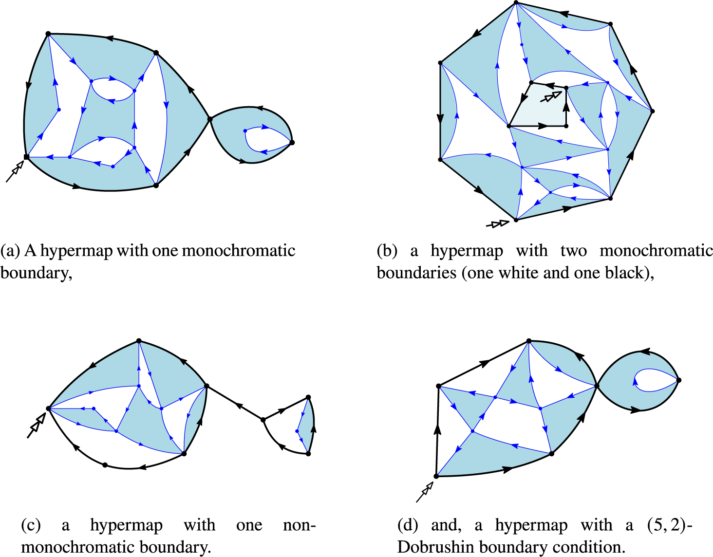
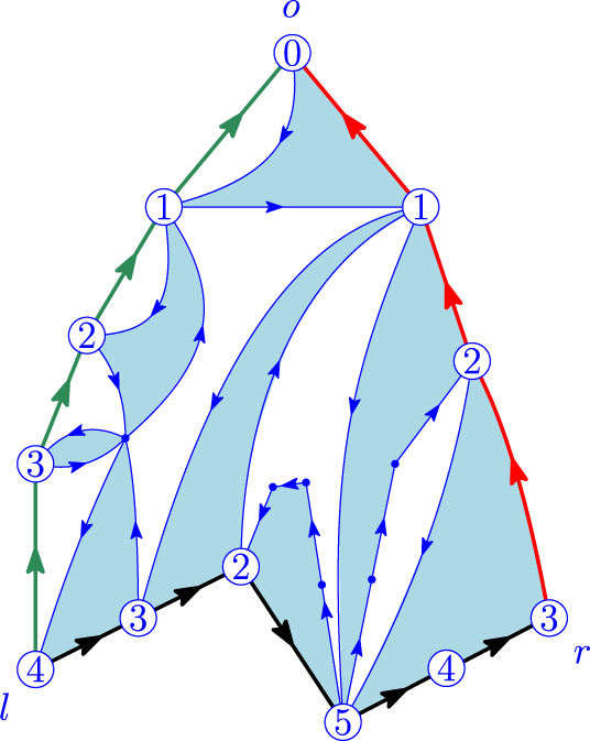


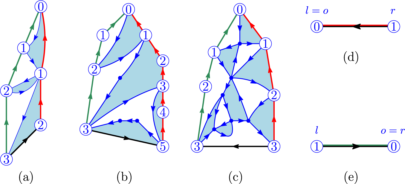


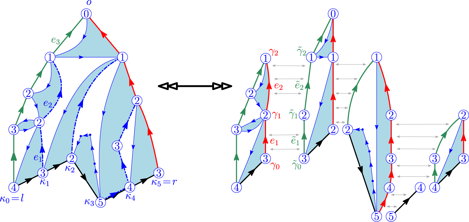


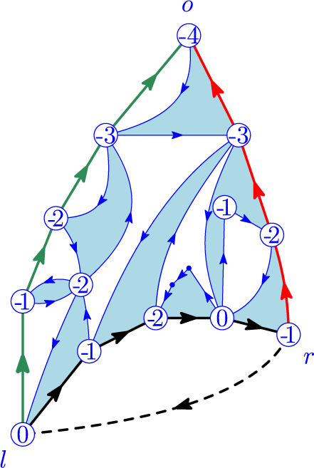


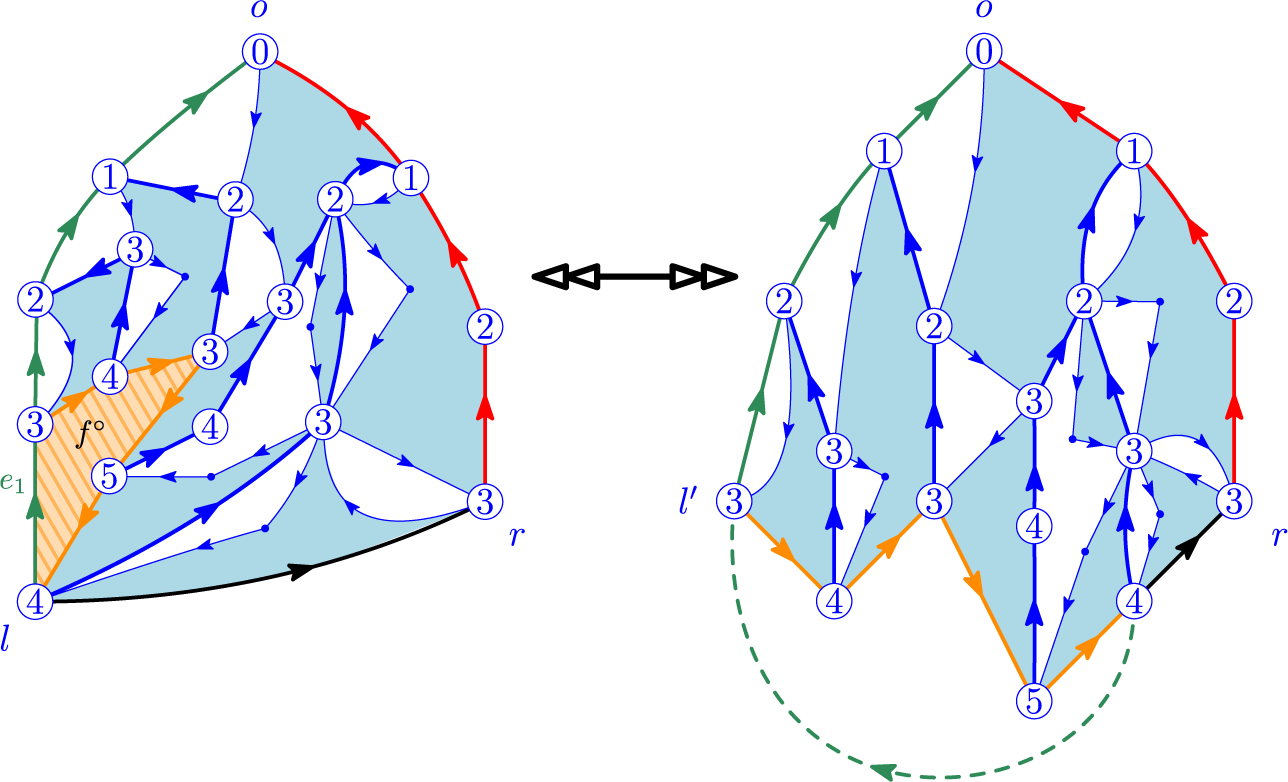


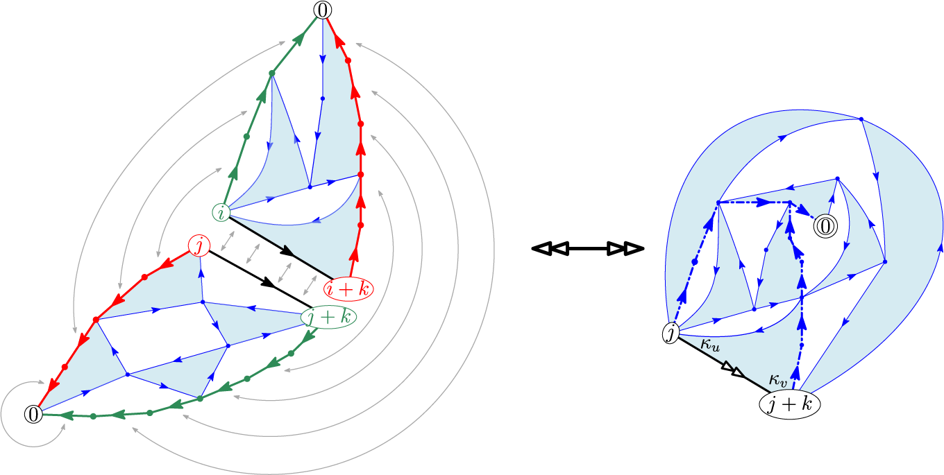


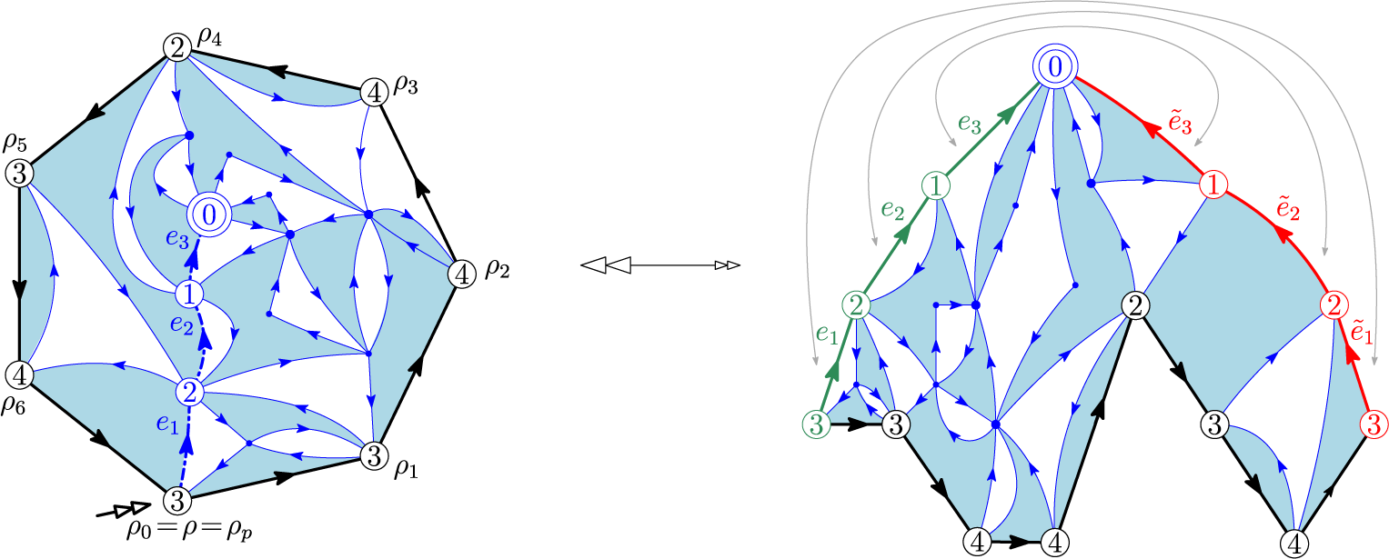

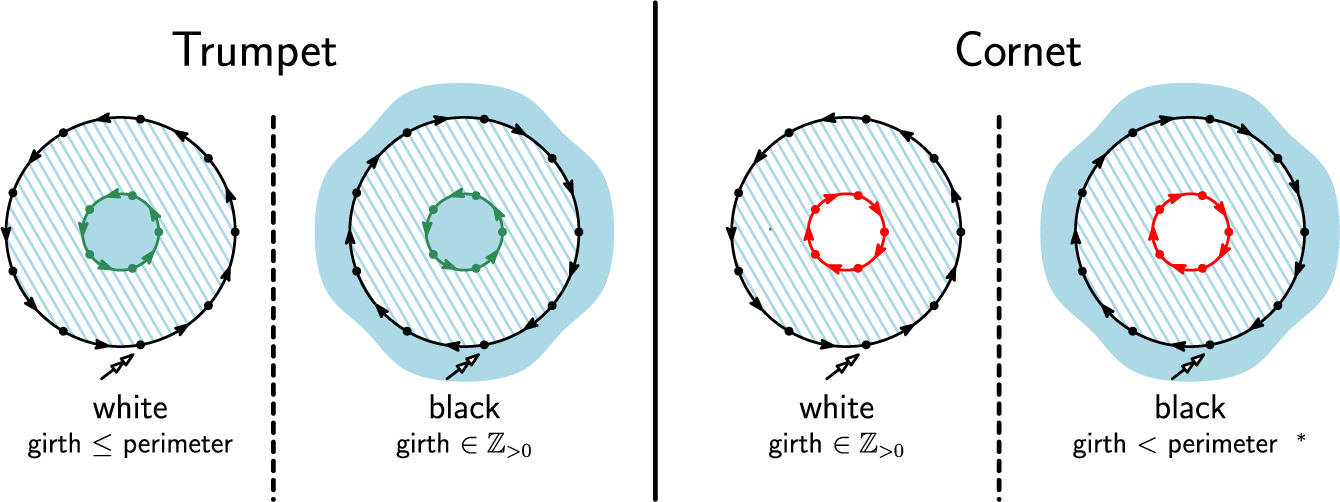


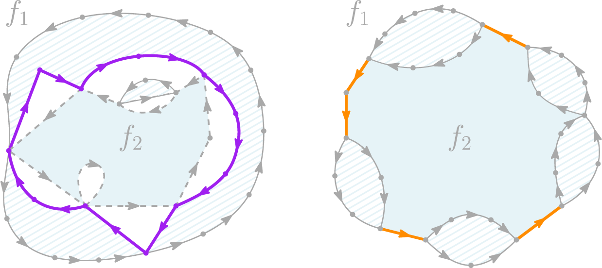





 Open access

