1 Introduction
Buoyancy-driven flow in permeable rock has been the focus of a considerable research effort given the importance of such effects for many environmental and energy-related processes, including enhanced oil recovery and carbon sequestration (Lake Reference Lake1989; Huppert & Woods Reference Huppert and Woods1995; Riaz et al.
Reference Riaz, Hesse, Tchelepi and Orr2006; Huppert & Neufeld Reference Huppert and Neufeld2014; Woods Reference Woods2014). Analyses have been carried out for relatively thin and hence confined aquifers and much deeper unconfined reservoirs, and the adjustment from an effectively unconfined flow at short times, to a confined flow at long times, was explored by Zheng et al. (Reference Zheng, Guo, Christov, Celia and Stone2015). The effects of a non-uniform viscosity ratio leads to the development of rarefaction waves and shocks (Lajeunesse et al.
Reference Lajeunesse, Martin, Rakotomalala, Salin and Yortsos1999; Juanes, MacMinn & Szulczewski Reference Juanes, MacMinn and Szulczewski2010; Gunn & Woods Reference Gunn and Woods2011), while the effects of the gradual dissolution of the
 $\text{CO}_{2}$
and capillary trapping of the
 $\text{CO}_{2}$
have been shown to cause the currents to gradually wane (Pruess et al.
Reference Pruess, García, Kovscek, Oldenburg, Rutqvist, Steefel and Xu2004; Hesse, Tchelepi & Orr Reference Hesse, Tchelepi and Orr2006). The role of capillary pressures impeding the advance of
 $\text{CO}_{2}$
through seal rock has also been explored (Woods & Farcas Reference Woods and Farcas2009) as well as the case in which fluid leaks off the current (Pritchard, Woods & Hogg Reference Pritchard, Woods and Hogg2001). Models have also been developed to account for two-phase flow effects (Golding et al.
Reference Golding, Neufeld, Hesse and Huppert2011).
The majority of these models have assumed that the formation is of uniform permeability. This leads to the simplifying result that the speed of the current is uniform with depth. However, in real geological strata, there are often multiple layers of different permeability. Reservoirs are typically made up of sedimentary rock that is very inhomogeneous and the contrasts in permeability can totally dominate fluid flow (Bjorlykke Reference Bjorlykke1993). Also within single geological flow units, such as are produced from massive turbidites flows on the sea-floor, the grain size is expected to gradually change with depth in the deposit as the parent turbulent flow either waxes or wanes.
While some of the effects of layering which can lead to the dispersion of buoyant plumes and gravity currents in a geological strata have been examined (Fayers, Blunt & Christie Reference Fayers, Blunt and Christie1992; Hesse & Woods Reference Hesse and Woods2010; Farcas & Woods Reference Farcas and Woods2016; Guo et al. Reference Guo, Bandilla, Nordbottten, Keilegavlen and Doster2016a ), there has been much less analysis of the effects of permeability gradients across an individual flow unit.
The purpose of this paper is to explore how a linear increase or decrease of permeability with height in a permeable layer influences the buoyancy-driven flow through that layer. The critical physical effect which this introduces is the variation of flow speed with vertical position in the layer, and we show that this can lead to some fundamentally different controls on the flow compared to a homogeneous reservoir.
In § 2, we introduce a model for a gravity-driven flow in a confined permeable rock in which the permeability varies with height. We then present some numerical solutions of the resulting nonlinear advection–diffusion equation for the evolution of the interface between the injected fluid and the original fluid in the system. This identifies that, under different conditions, there are rarefaction-wave-type solutions, travelling-wave-type solutions and mixtures of these solutions at different depths in the layer. We then compare long-time asymptotic rarefaction-wave and travelling-wave solutions of the governing equation with the full numerical solutions. We discuss the implications of these results, in comparison with the very different current structure that develops in a homogeneous porous layer, when each fluid has the same viscosity, in which the front of the flow spreads at a rate proportional to
 $t^{1/2}$
. In § 4 we develop a short-time asymptotic analysis of the governing equation, following the approach of Zheng et al. (Reference Zheng, Guo, Christov, Celia and Stone2015). We analyse how a permeability gradient and viscosity ratio affect the early-time behaviour which asymptotes to that of an unconfined gravity current.
We conclude with a discussion focusing on the challenges of predicting the storage capacity of an aquifer by illustrating how the fraction of the pore space that may be flooded with
 $\text{CO}_{2}$
varies if we account for cross-layer variations in permeability, and illustrating that, with more complex vertical structure for the permeability, it is possible to have multiple shock regions separated by rarefaction-wave regions.
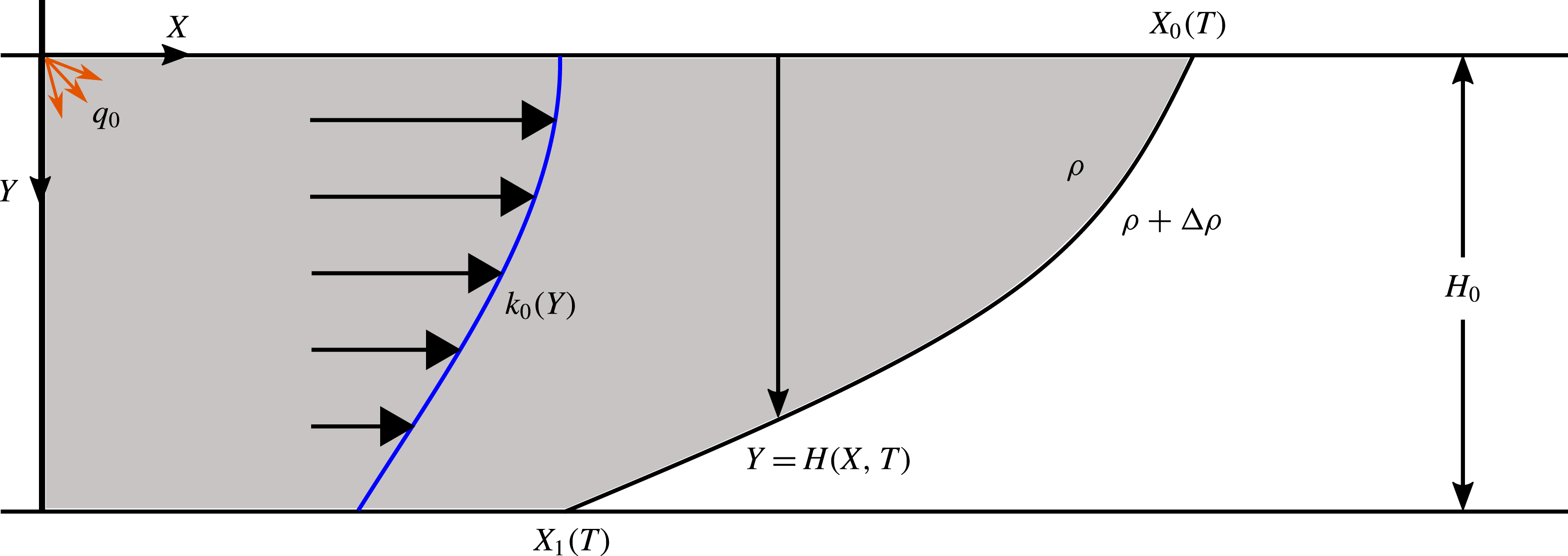
Schematic diagram showing the model problem for constant injection into a vertically heterogeneous aquifer.

2 Model
We assume liquid of density
 $\unicode[STIX]{x1D70C}$
and viscosity
 $\unicode[STIX]{x1D707}_{i}$
is injected into a horizontal, laterally extensive aquifer initially filled with liquid of density
 $\unicode[STIX]{x1D70C}+\unicode[STIX]{x0394}\unicode[STIX]{x1D70C}$
and viscosity
 $\unicode[STIX]{x1D707}_{a}$
(figure 1). The aquifer has depth
 $H_{0}$
and porosity
 $\unicode[STIX]{x1D719}$
, and fluid is injected at
 $X=0$
,
 $Y=0$
with a flow rate
 $q_{0}$
. The vertically varying permeability
 $k_{0}(Y)$
is independent of horizontal position. In the region where the aquifer is fully flooded by the injected fluid, the flow will be pressure-driven, whilst in the slumping region between the two contact points, flow will be driven by a mixture of buoyancy and the background pressure gradient. We assume that the fluids are incompressible, that the motion is governed by Darcy’s law and that there is a sharp interface between the immiscible fluids. Once the invading fluid has spread beyond a distance
 $L\gg H_{0}$
from the well, the pressure becomes approximately hydrostatic (Bear Reference Bear1971; Huppert & Woods Reference Huppert and Woods1995) and is given by
 $$\begin{eqnarray}\displaystyle P(X,Y,T)=\left\{\begin{array}{@{}ll@{}}P_{0}+\unicode[STIX]{x1D70C}gY, & 0<Y<H,\\ P_{0}+(\unicode[STIX]{x1D70C}+\unicode[STIX]{x0394}\unicode[STIX]{x1D70C})gY-\unicode[STIX]{x0394}\unicode[STIX]{x1D70C}gH, & H<Y<H_{0},\end{array}\right. & & \displaystyle\end{eqnarray}$$
where
 $P_{0}=P(X,0,T)$
is the unknown pressure at the top of the aquifer. Using Darcy’s law for the horizontal component of the flow,
 $$\begin{eqnarray}\displaystyle & \displaystyle u_{i}=-{\displaystyle \frac{k_{0}(Y)}{\unicode[STIX]{x1D707}_{i}}}{\displaystyle \frac{\unicode[STIX]{x2202}P_{0}}{\unicode[STIX]{x2202}X}},\quad u_{a}=-{\displaystyle \frac{k_{0}(Y)}{\unicode[STIX]{x1D707}_{a}}}\left({\displaystyle \frac{\unicode[STIX]{x2202}P_{0}}{\unicode[STIX]{x2202}X}}-\unicode[STIX]{x0394}\unicode[STIX]{x1D70C}g{\displaystyle \frac{\unicode[STIX]{x2202}H}{\unicode[STIX]{x2202}X}}\right), & \displaystyle\end{eqnarray}$$
where
 $u_{i}$
and
 $u_{a}$
are the transport velocities of the injectate and ambient fluid, respectively. Local mass conservation for the injected and ambient fluids may be expressed in the form
 $$\begin{eqnarray}\displaystyle & \displaystyle \unicode[STIX]{x1D719}{\displaystyle \frac{\unicode[STIX]{x2202}H}{\unicode[STIX]{x2202}T}}=-{\displaystyle \frac{\unicode[STIX]{x2202}}{\unicode[STIX]{x2202}X}}\left(\int _{0}^{H}u_{i}\,\text{d}Y\right),\quad \unicode[STIX]{x1D719}{\displaystyle \frac{\unicode[STIX]{x2202}(H_{0}-H)}{\unicode[STIX]{x2202}T}}=-{\displaystyle \frac{\unicode[STIX]{x2202}}{\unicode[STIX]{x2202}X}}\left(\int _{H}^{H_{0}}u_{a}\,\text{d}Y\right). & \displaystyle\end{eqnarray}$$
Adding these two equations together provides an equation for the conservation of mass of the current,
 $$\begin{eqnarray}\displaystyle & \displaystyle \int _{0}^{H}u_{i}\,\text{d}Y+\int _{H}^{H_{0}}u_{a}\,\text{d}Y=q_{0}. & \displaystyle\end{eqnarray}$$
This can be recast as a constraint for the global mass conservation of the injected fluid,
 $$\begin{eqnarray}\displaystyle & \displaystyle \unicode[STIX]{x1D719}\int _{0}^{X_{0}(t)}H(X,T)\,\text{d}X=q_{0}T, & \displaystyle\end{eqnarray}$$
where
 $X_{0}(T)$
is the contact point along the top of the aquifer (see figure 1), and we have assumed injection begins at
 $T=0$
. We use the aquifer height
 $H_{0}$
and the vertically averaged permeability,
 $$\begin{eqnarray}\displaystyle & \displaystyle \bar{k}={\displaystyle \frac{1}{H_{0}}}\int _{0}^{H_{0}}k_{0}(Y)\,\text{d}Y, & \displaystyle\end{eqnarray}$$
to introduce the dimensionless quantity
 $$\begin{eqnarray}\displaystyle & \displaystyle K_{0}(H)={\displaystyle \frac{1}{H_{0}\bar{k}}}\int _{0}^{H}k_{0}(Y)\,\text{d}Y. & \displaystyle\end{eqnarray}$$
Note that
 $K_{0}(0)=0$
,
 $K_{0}(H_{0})=1$
and, in a uniform aquifer,
 $K_{0}(H)=H/H_{0}$
. The unknown pressure
 $P_{0}$
can be eliminated by substituting the expressions for the Darcy velocities (2.2) into (2.4). Local mass conservation for the injectate (2.3a
) then leads to the advection–diffusion type equation for the depth of the current,
 $$\begin{eqnarray}\displaystyle & & \displaystyle \displaystyle \unicode[STIX]{x1D719}{\displaystyle \frac{\unicode[STIX]{x2202}H}{\unicode[STIX]{x2202}T}}+q_{0}{\displaystyle \frac{\unicode[STIX]{x2202}}{\unicode[STIX]{x2202}X}}\left({\displaystyle \frac{K_{0}(H)}{K_{0}(H)+M(1-K_{0}(H))}}\right)\nonumber\\ \displaystyle & & \displaystyle \quad =UH_{0}{\displaystyle \frac{\unicode[STIX]{x2202}}{\unicode[STIX]{x2202}X}}\left({\displaystyle \frac{MK_{0}(H)(1-K_{0}(H))}{K_{0}(H)+M(1-K_{0}(H))}}{\displaystyle \frac{\unicode[STIX]{x2202}H}{\unicode[STIX]{x2202}X}}\right),\end{eqnarray}$$
where
 $$\begin{eqnarray}\displaystyle & \displaystyle U={\displaystyle \frac{\unicode[STIX]{x0394}\unicode[STIX]{x1D70C}g\bar{k}}{\unicode[STIX]{x1D707}_{i}}},\quad M={\displaystyle \frac{\unicode[STIX]{x1D707}_{i}}{\unicode[STIX]{x1D707}_{a}}} & \displaystyle\end{eqnarray}$$
are the velocity associated with the buoyant slumping of the injectate, and the viscosity ratio, respectively. To complete the mathematical description, we require initial and boundary conditions. Injection begins at
 $T=0$
so
 $$\begin{eqnarray}\displaystyle H(X,0)=0. & & \displaystyle\end{eqnarray}$$
At the contact point along the top of the aquifer,
 $X=X_{0}(T)$
, the boundary condition is
 $$\begin{eqnarray}\displaystyle H(X_{0}(T),T)=0. & & \displaystyle\end{eqnarray}$$
Differentiating the equation for mass conservation (2.5) with respect to time and applying the boundary condition (2.11) gives
 $$\begin{eqnarray}\displaystyle & \displaystyle \unicode[STIX]{x1D719}\int _{0}^{X_{0}(t)}{\displaystyle \frac{\unicode[STIX]{x2202}H}{\unicode[STIX]{x2202}T}}\,\text{d}X=q_{0}. & \displaystyle\end{eqnarray}$$
By integrating (2.8) between
 $X=0$
and
 $X=X_{0}(T)$
, and applying (2.11) and (2.12), we obtain the boundary condition at
 $X=0$
:
 $$\begin{eqnarray}\displaystyle & \displaystyle \Bigg[q_{0}{\displaystyle \frac{K_{0}(H)}{K_{0}(H)+M(1-K_{0}(H))}}-UH_{0}{\displaystyle \frac{MK_{0}(H)(1-K_{0}(H))}{K_{0}(H)+M(1-K_{0}(H))}}{\displaystyle \frac{\unicode[STIX]{x2202}H}{\unicode[STIX]{x2202}X}}\Bigg]\Bigg|_{X=0}=q_{0}.\qquad & \displaystyle\end{eqnarray}$$
Note that the governing equation (2.8) and the boundary conditions (2.11) and (2.13) do not change when the aquifer becomes fully flooded by the injectate.
2.1 Non-dimensionalisation
Balancing the contributions from the net flow and the buoyant slumping in the nose region of the current leads to the scalings
 $$\begin{eqnarray}\displaystyle & \displaystyle h={\displaystyle \frac{H}{H_{0}}},\quad y={\displaystyle \frac{Y}{H_{0}}},\quad x={\displaystyle \frac{q_{0}}{UH_{0}^{2}}}X,\quad t={\displaystyle \frac{q_{0}^{2}}{\unicode[STIX]{x1D719}UH_{0}^{3}}}T. & \displaystyle\end{eqnarray}$$
Using these scalings and the functions
 $$\begin{eqnarray}\displaystyle k(y)={\displaystyle \frac{k_{0}(Y)}{\bar{k}}},\quad K(y)=K_{0}(Y), & & \displaystyle\end{eqnarray}$$
we can re-express (2.8) in dimensionless form as
 $$\begin{eqnarray}\displaystyle {\displaystyle \frac{\unicode[STIX]{x2202}h}{\unicode[STIX]{x2202}t}}+{\displaystyle \frac{\unicode[STIX]{x2202}}{\unicode[STIX]{x2202}x}}\Bigg({\displaystyle \frac{K(h)}{K(h)+M(1-K(h))}}\Bigg)={\displaystyle \frac{\unicode[STIX]{x2202}}{\unicode[STIX]{x2202}x}}\Bigg({\displaystyle \frac{MK(h)(1-K(h))}{K(h)+M(1-K(h))}}{\displaystyle \frac{\unicode[STIX]{x2202}h}{\unicode[STIX]{x2202}x}}\Bigg). & & \displaystyle\end{eqnarray}$$
Our choice of scalings (2.14) has removed the buoyancy parameter,
 $$\begin{eqnarray}\displaystyle B={\displaystyle \frac{q_{0}}{UH_{0}}}, & & \displaystyle\end{eqnarray}$$
from the governing equation so that, in dimensionless terms, buoyancy dominates for
 $t\ll 1$
and the net flow driven by pressure for
 $t\gg 1$
. The initial condition is
 $h(x,0)=0$
. The boundary condition at the leading contact point,
 $x=x_{0}(t)$
, is
 $h(x_{0}(t),t)=0$
. The dimensionless form of the
 $X=0$
boundary condition (2.13) is
 $$\begin{eqnarray}\displaystyle & \displaystyle \Bigg[{\displaystyle \frac{K(h)}{K(h)+M(1-K(h))}}-{\displaystyle \frac{MK(h)(1-K(h))}{K(h)+M(1-K(h))}}{\displaystyle \frac{\unicode[STIX]{x2202}h}{\unicode[STIX]{x2202}x}}\Bigg]\Bigg|_{x=0}=1. & \displaystyle\end{eqnarray}$$
At early times, when the aquifer has not been fully flooded by the injectate and
 $h(0,t)<1$
, the boundary condition (2.18) can be rearranged. First, we multiply by
 $K(h)+M(1-K(h))$
, the
 $K(h)$
terms then cancel, and dividing by
 $M(1-K(h))$
gives
 $$\begin{eqnarray}\displaystyle & \displaystyle 1=\Bigg[-K(h){\displaystyle \frac{\unicode[STIX]{x2202}h}{\unicode[STIX]{x2202}x}}\Bigg]\Bigg|_{x=0}. & \displaystyle\end{eqnarray}$$
At later times
 $h(0,t)=1$
and such a rearrangement is not possible because the last step was dividing by
 $M(1-K(h))$
. Instead, we observe that
 $h=1$
satisfies (2.18) for any value of
 $\unicode[STIX]{x2202}h/\unicode[STIX]{x2202}x$
. The flooding of the aquifer implies a second contact point at the base of the aquifer with
 $h(x_{1}(t),t)=1,$
where
 $x_{1}(t)<x_{0}(t)$
(see figure 1).
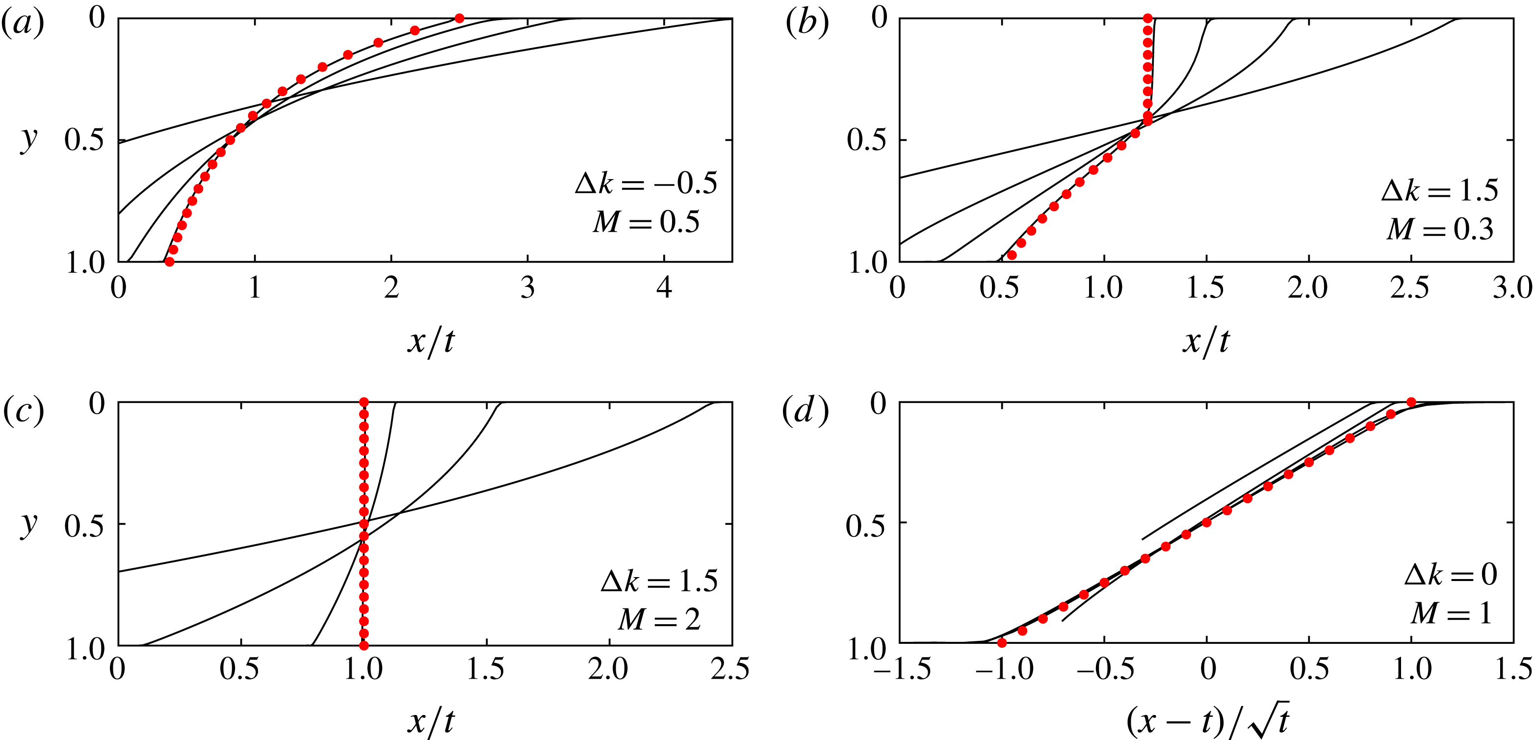
Numerical simulations of the injection of buoyant fluid into a stratified porous medium from early to late times. The interface is shown at
 $t=0.1$
,
 $0.5$
,
 $2.5$
and
 $62.5$
in similarity coordinates for four different sets of parameter values (a–d). The late-time asymptotic solutions found in § 5 are shown as red dots and they agree well with the
 $t=62.5$
numerical solution. Panel (a) shows a rarefaction wave, the asymptotic shape being given by (5.7); (b) is a compound interface with shock and rarefaction regions, the shape of the shock being given by (5.19); (c) is a full shock, with shape given by (5.11); and (d) is the case of uniform permeability and equal viscosities, which leads to a front that grows in proportion to
 $t^{1/2}$
, the shape found by Huppert & Woods (Reference Huppert and Woods1995). These four panels characterise the four possible late-time regimes, shown in parameter space in figure 4.

3 Numerical simulation
We conducted direct numerical simulations of the nonlinear advection–diffusion equation (2.16) with appropriate boundary conditions following the approach of Zheng et al. (Reference Zheng, Guo, Christov, Celia and Stone2015) using the finite difference scheme of Kurganov & Tadmor (Reference Kurganov and Tadmor2000). Whilst the model in § 2 applies for any
 $k(y)$
, we first choose to use a linear stratification,
 $$\begin{eqnarray}\displaystyle & \displaystyle k(y)=1+\unicode[STIX]{x0394}k(y-{\textstyle \frac{1}{2}}). & \displaystyle\end{eqnarray}$$
Here
 $\unicode[STIX]{x0394}k=k(1)-k(0)$
is the dimensionless permeability difference between the top and the base of the aquifer, and has values in the range
 $-2<\unicode[STIX]{x0394}k<2$
.
Figure 2 shows the numerical results at early and late times, illustrating how the interface transitions to the late-time solution (red dots). The long-time solutions are independent of the vertical location of the injection well at
 $x=0$
because the injectate has flooded the aquifer. However, at early times the injection height is critical. For our model, we have assumed the injection well is located at
 $x=0$
,
 $y=0$
. In the early time period, when the current is thin and the interface has not made contact with the lower boundary, we expect that the governing equation (2.16) can be simplified and that the flow resembles that in an unconfined aquifer. This is studied in § 4 in which we develop early-time asymptotic solutions and compare these with our numerical simulations (see figure 3). If the fluid was injected at
 $y=1$
, the initial flow would form a buoyant plume, leading to a different adjustment towards the gravity-driven flow (see Lyu & Woods Reference Lyu and Woods2016). The plume head would develop irregular fingers as it advances towards the top boundary of the aquifer. The injectate subsequently fills the depth of the aquifer in the region near the source and the evolution transitions to the fully flooded late-time regimes described in § 5.
Figure 2 illustrates the four late-time regimes for the interface. Figure 2(a) is a growing rarefaction wave across the whole aquifer, which may be identified since the horizontal coordinate is
 $x/t$
; figure 2(b) shows a compound interface consisting of a vertical interface in the upper region, which travels at a constant speed
 $V$
, and a growing rarefaction wave in the lower region. In figure 2(c), the shock extends across the entire aquifer and travels with unit velocity; figure 2(d) is the special case of uniform permeability and unit viscosity ratio, for which the interface grows proportionally to
 $t^{1/2}$
as found by Pegler, Huppert & Neufeld (Reference Pegler, Huppert and Neufeld2014) and Zheng et al. (Reference Zheng, Guo, Christov, Celia and Stone2015). These numerical results motivate the late-time asymptotic analysis of the four regimes in § 5, which suggests parameter values for which each regime occurs (see figure 4).
4 Early-time asymptotic solutions
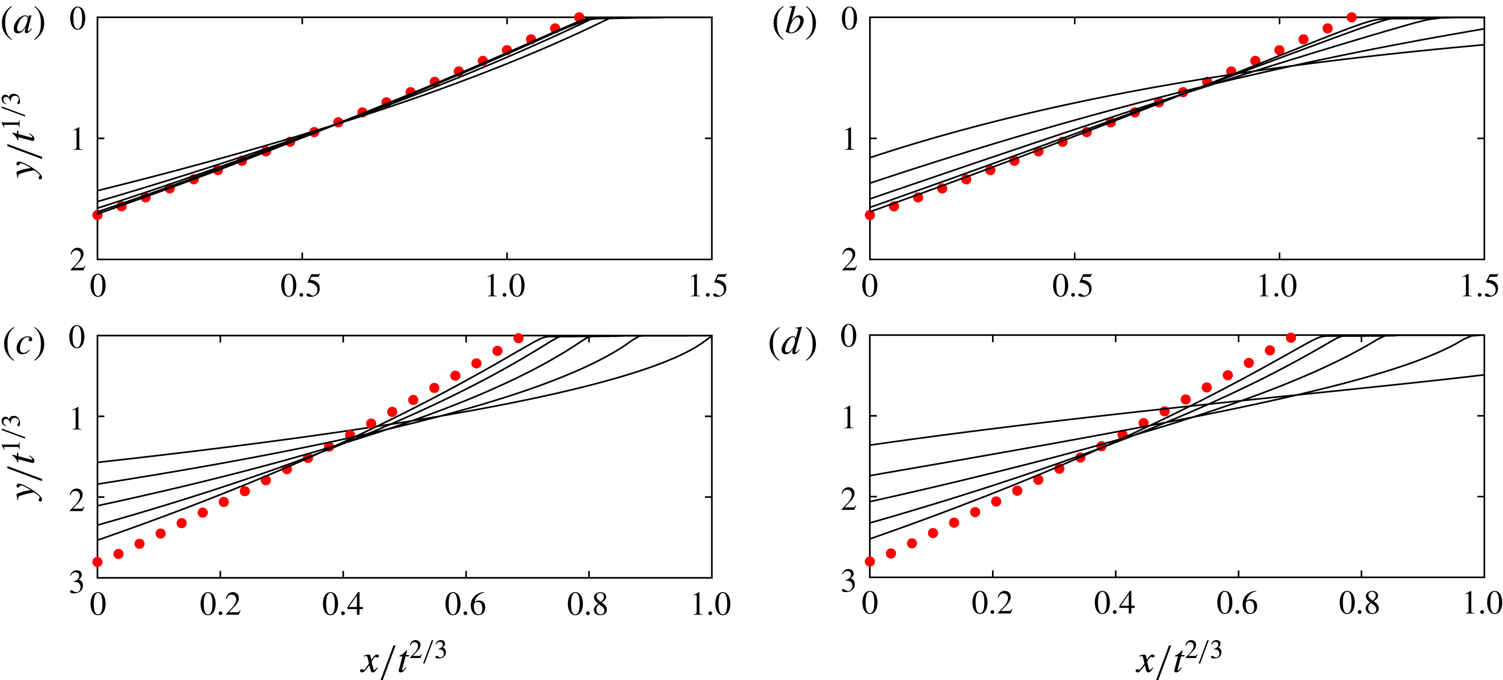
Early evolution of the interface at five times:
 $t=10^{-5}$
to
 $t=10^{-1}$
. The similarity solution found in § 4 is shown in red dots. (a,b) The results for
 $\unicode[STIX]{x0394}k=1$
and
 $M=10$
and
 $0.1$
, demonstrating how the early time period is controlled by
 $M$
. (c,d) The results for
 $\unicode[STIX]{x0394}k=1.8$
and
 $M=10$
and
 $0.1$
, showing similar divergence rates because, when
 $M\geqslant k(0)$
, the early time period is independent of
 $M$
.

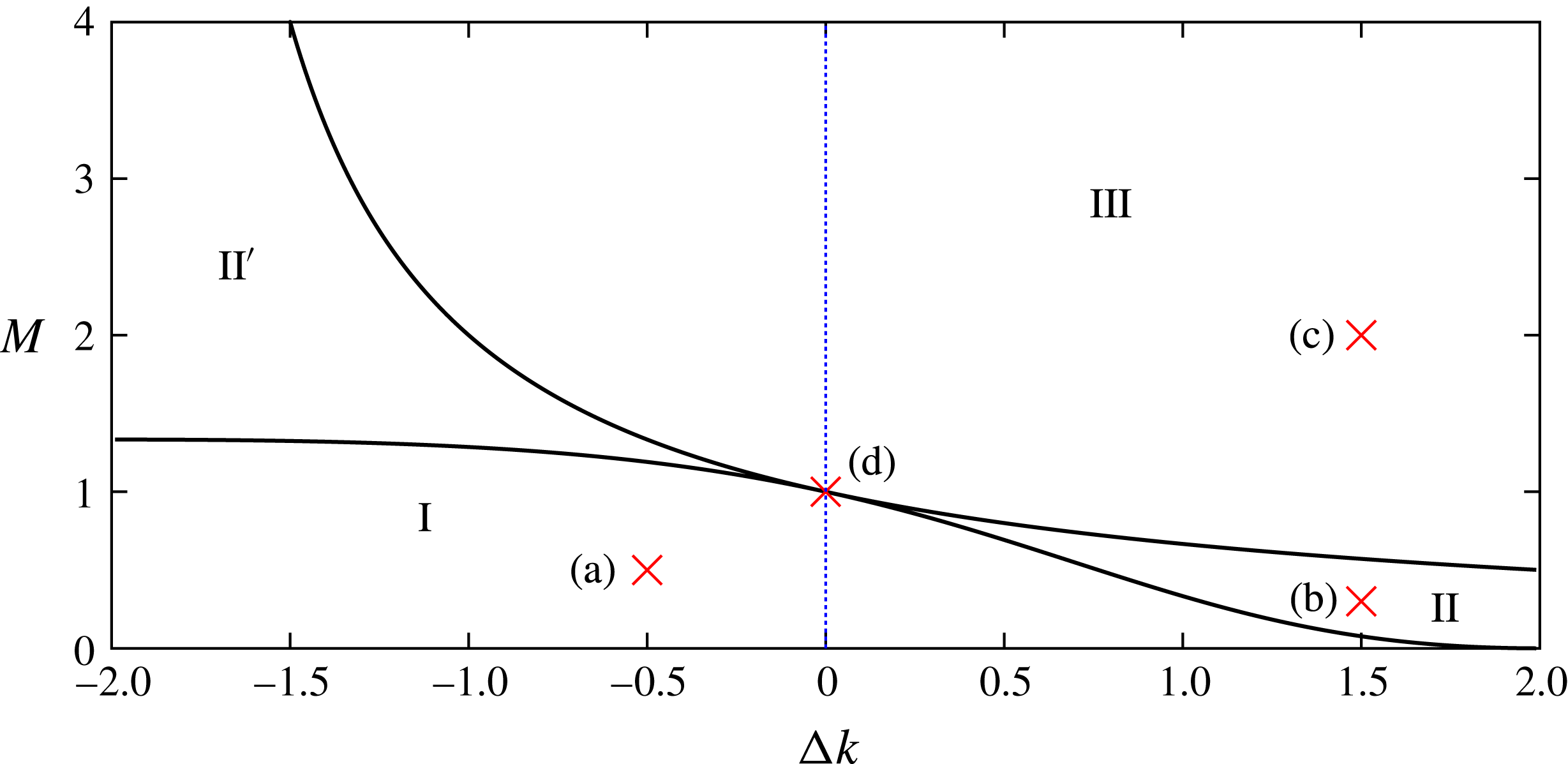
Parameter space for late-time solution for linear
 $k(y)$
. For parameter values in region I, given by (5.6), the interface tends to a rarefaction wave (figure 2
a). In region III, given by (5.9), the interface develops a shock across the entire aquifer (figure 2
c). For regions II and II
 $^{\prime }$
, there is a mixed solution (figure 2
b). The blue dashed line along
 $\unicode[STIX]{x0394}k=0$
is the region of parameter space previously studied by Pegler et al. (Reference Pegler, Huppert and Neufeld2014) and Zheng et al. (Reference Zheng, Guo, Christov, Celia and Stone2015); the solution at
 $\unicode[STIX]{x0394}k=0$
,
 $M=1$
(see figure 2
d) where the interface grows proportional to
 $t^{1/2}$
is shown to be singular by this figure. Moreover, by including heterogeneous permeability, we have found new compound solutions in regions II and II
 $^{\prime }$
which do not occur along the blue dashed line. The labelled red crosses correspond to the parameter values for the interface shapes in the panels (a–d) in figure 2.

In this section, we show that the early-time evolution is controlled primarily by the permeability at the top of the aquifer and the viscosity ratio. The early regime is valid until
 $t=O(0.1)$
, which corresponds to the first few weeks of injection in a typical
 $\text{CO}_{2}$
storage project (see § 7).
At early times, with the injection well located at the origin, the fluid–fluid interface does not touch the lower boundary of the aquifer and
 $h$
is small everywhere. The injectate forms a thin layer at the top of the aquifer and the flow initially resembles an unconfined gravity-driven flow (cf. Huppert & Woods Reference Huppert and Woods1995). The ratio of the buoyancy force to the pressure associated with the net flow is large at early times and hence the advection term can be neglected. Linearising in
 $K(h)$
, the full governing equation (2.16) may be approximated by the equation
 $$\begin{eqnarray}\displaystyle & \displaystyle {\displaystyle \frac{\unicode[STIX]{x2202}h}{\unicode[STIX]{x2202}t}}=k(0){\displaystyle \frac{\unicode[STIX]{x2202}}{\unicode[STIX]{x2202}x}}\left(h{\displaystyle \frac{\unicode[STIX]{x2202}h}{\unicode[STIX]{x2202}x}}\right). & \displaystyle\end{eqnarray}$$
The early-time solution is independent of the viscosity ratio since, in this limit, the displacement of the original fluid in the aquifer is not rate-limiting. The only parameter in (4.1) is
 $k(0)$
. We anticipate that the value of the permeability at only
 $y=0$
is sufficient to describe the early-time regime.
The diffusion equation (4.1) has been well studied by Barenblatt (Reference Barenblatt1952), Hesse et al. (Reference Hesse, Tchelepi, Cantwel and Orr2007) and MacMinn et al. (Reference MacMinn, Neufeld, Hesse and Huppert2012). For injection with a constant flux, it admits a similarity solution with similarity coordinate
 $\unicode[STIX]{x1D702}=x/(\sqrt{3k(0)}\,t^{2/3})$
. The leading contact point at the top of the aquifer propagates as
 $x_{0}=\unicode[STIX]{x1D702}_{0}\sqrt{3k(0)}\,t^{2/3}$
, where
 $\unicode[STIX]{x1D702}_{0}$
is to be determined. If we rescale the system, then
 $s=x/x_{0}=\unicode[STIX]{x1D702}/\unicode[STIX]{x1D702}_{0}$
, so that the contact point is at
 $s=1$
and the depth of the current can be written as
 $$\begin{eqnarray}\displaystyle h=\unicode[STIX]{x1D702}_{0}^{2}t^{1/3}\unicode[STIX]{x1D713}(s). & & \displaystyle\end{eqnarray}$$
Here
 $\unicode[STIX]{x1D713}$
is the shape function, which satisfies
 $$\begin{eqnarray}\displaystyle \left.\begin{array}{@{}c@{}}\unicode[STIX]{x1D713}-2s{\displaystyle \frac{\text{d}\unicode[STIX]{x1D713}}{\text{d}s}}={\displaystyle \frac{\text{d}}{\text{d}s}}\left(\unicode[STIX]{x1D713}{\displaystyle \frac{\text{d}\unicode[STIX]{x1D713}}{\text{d}s}}\right),\\[12.0pt] \unicode[STIX]{x1D713}(1)=0.\end{array}\right\} & & \displaystyle\end{eqnarray}$$
Global mass conservation identifies that the contact point is given by
 $$\begin{eqnarray}\displaystyle & \displaystyle \unicode[STIX]{x1D702}_{0}=\Bigg(\sqrt{3k(0)}\int _{0}^{1}\unicode[STIX]{x1D713}(s)\,\text{d}s\Bigg)^{-1/3}. & \displaystyle\end{eqnarray}$$
To solve the ordinary differential equation (4.3) numerically, a second boundary condition is required. Letting
 $s\rightarrow 1^{-}$
gives
 $\unicode[STIX]{x1D713}(s)\approx 2(1-s)$
, providing the boundary conditions used in the numerical procedure:
 $\unicode[STIX]{x1D713}^{\prime }(1-\unicode[STIX]{x1D716})\approx 2$
,
 $\unicode[STIX]{x1D713}(1-\unicode[STIX]{x1D716})\approx 2\unicode[STIX]{x1D716}$
, where
 $\unicode[STIX]{x1D716}\ll 1$
. Solving for
 $\unicode[STIX]{x1D713}$
gives
 $h(0,t)=1.298(t/k(0))^{1/3}$
. The numerical solutions to (4.3) are shown in figure 3.
The solutions are valid provided both
 $h\ll 1$
and
 $M(\unicode[STIX]{x2202}h/\unicode[STIX]{x2202}x)\gg 1$
(so that buoyancy dominates). The first condition is equivalent to
 $t\ll k(0)$
, whilst the second requires
 $t\ll M^{3}/k(0)^{2}$
. If
 $M=O(k(0))$
then these times are similar. For
 $M\gg k(0)$
, the early time period is controlled by the first condition, and for
 $M\ll k(0)$
, it is controlled by the second (see figure 3). When the aquifer has a much higher permeability at the top than the bottom (i.e.
 $k(0)$
larger), the early-time solution is valid for longer because the injectate can easily migrate along the top of the aquifer driven by the buoyancy, and the influence of the pressure gradient associated with the net flow is less significant in this high-permeability region (figure 3
a,b). Conversely, for a channel with low permeability at the top, the buoyancy forces are less effective at shearing out the flow, and the pressure gradient associated with the net flow becomes important earlier. As a result, the approximation
 $h\ll 1$
breaks down earlier (see figure 3
c,d). Previous studies have shown that the length of the early time period increases strongly with
 $M$
up to
 $M\sim 1$
in a uniform aquifer (MacMinn & Juanes Reference MacMinn and Juanes2009), and our contribution demonstrates that this relationship is valid until
 $M\sim k(0)$
for aquifers with a linear permeability gradient.
After the initial transient in which (4.2) is valid, there is an adjustment regime as the depth of the current increases until it fully floods the aquifer, and the long-time asymptotics apply as explored in § 5.
5 Late-time asymptotic solutions
At long times, the permeability profile across the aquifer has a significant influence on the interface evolution, in contrast to the early-time evolution. We anticipate that the lateral extent of the current is very large compared to the depth of the layer. This implies that the ratio of the buoyancy force to the pressure associated with the net flow is small. In dimensional terms, this is equivalent to
 $$\begin{eqnarray}\displaystyle & \displaystyle {\displaystyle \frac{MH_{0}}{L}}\ll 1, & \displaystyle\end{eqnarray}$$
where
 $L$
is the length of the interface. The diffusive term on the right-hand side of (2.16) can then be neglected. We therefore seek solutions to the equation
 $$\begin{eqnarray}\displaystyle & \displaystyle {\displaystyle \frac{\unicode[STIX]{x2202}h}{\unicode[STIX]{x2202}t}}+{\displaystyle \frac{\unicode[STIX]{x2202}}{\unicode[STIX]{x2202}x}}\left({\displaystyle \frac{K(h)}{K(h)+M(1-K(h))}}\right)=0, & \displaystyle\end{eqnarray}$$
with boundary conditions
 $h(x_{0}(t),t)=0$
and
 $h(0,t)=1$
since the aquifer is fully flooded. This is a scalar first-order linear equation with flux function (see sec. 4 of Juanes et al.
Reference Juanes, MacMinn and Szulczewski2010),
 $$\begin{eqnarray}\displaystyle F(h)={\displaystyle \frac{K(h)}{K(h)+M(1-K(h))}}. & & \displaystyle\end{eqnarray}$$
The characteristics are
 $$\begin{eqnarray}\displaystyle & \displaystyle {\displaystyle \frac{\text{d}x}{\text{d}t}}=F^{\prime }(h_{0}(s))={\displaystyle \frac{Mk(h_{0}(s))}{[K(h_{0}(s))+M(1-K(h_{0}(s)))]^{2}}}, & \displaystyle\end{eqnarray}$$
where
 $h=h_{0}(s)$
is the general initial condition on the line
 $x=s$
,
 $t=0$
in the (
 $x,t$
) plane and
 $h_{0}(s)$
is a decreasing function. The initial conditions develop into either a shock or a rarefaction wave.
5.1 Rarefaction interface
If
 $F^{\prime }(h)$
is monotonically decreasing in
 $(0,1)$
, then the Jacobian is nowhere zero and the method of characteristics can be applied to solve (5.2). For the linear
 $k(y)$
given by (3.1), we wish to find values of the parameters
 $\unicode[STIX]{x0394}k$
and
 $M$
for which this solution method is possible and the interface is a rarefaction. The condition that
 $F^{\prime }(h)$
is monotonically decreasing across the channel is equivalent to requiring
 $$\begin{eqnarray}\displaystyle & \displaystyle F^{\prime \prime }(h)\equiv {\displaystyle \frac{M\unicode[STIX]{x0394}k[K(h)+M(1-K(h))]-2M(1-M)k(h)^{2}}{[K(h)+M(1-K(h))]^{3}}} & \displaystyle\end{eqnarray}$$
to be negative in all of
 $(0,1)$
. The denominator is always positive across the channel and the numerator is a quadratic in
 $h$
since
 $k(h)$
is linear. The condition for the rarefaction solution can now be found in terms of the parameters,
 $$\begin{eqnarray}\displaystyle & \displaystyle M\leqslant {\displaystyle \frac{(\unicode[STIX]{x0394}k-2)^{2}}{\unicode[STIX]{x0394}k^{2}-2\unicode[STIX]{x0394}k+4}}. & \displaystyle\end{eqnarray}$$
Equation (5.2) then has self-similar solutions
 $h(x,t)=h(\unicode[STIX]{x1D709})$
, in terms of the similarity variable
 $\unicode[STIX]{x1D709}=x/t$
. The solution is implicitly given by
 $$\begin{eqnarray}\displaystyle & \displaystyle \unicode[STIX]{x1D709}={\displaystyle \frac{x}{t}}=F^{\prime }(h), & \displaystyle\end{eqnarray}$$
and the contact points satisfy
 $$\begin{eqnarray}\displaystyle & \displaystyle x_{0}(t)={\displaystyle \frac{\left(1-{\textstyle \frac{1}{2}}\unicode[STIX]{x0394}k\right)t}{M}},\quad x_{1}(t)=M(1+{\textstyle \frac{1}{2}}\unicode[STIX]{x0394}k)t, & \displaystyle\end{eqnarray}$$
at
 $h=0$
and
 $h=1$
, respectively. Provided the inequality (5.6) is satisfied,
 $h$
is a decreasing function of
 $x$
and the extent of the interface grows in proportion to time, implying that the diffusive term in the governing equation (2.16) is
 $O(t^{-2})$
whilst the advection term is
 $O(t^{-1})$
. The interface gradient is
 $O(t^{-1})$
and the assumptions made in arriving at (5.2) are self-consistent. This analysis is confirmed by comparing the asymptotic solution (5.7), with numerical simulations of the full governing equation in figure 2(a).
Figure 4 shows the region I in parameter space given by (5.6). If the injectate is sufficiently mobile compared to the ambient fluid (
 $M\ll 1$
), then the current will run along a thin layer at the top, even if the permeability is much lower there (i.e.
 $\unicode[STIX]{x0394}k\approx 2$
). Conversely, when
 $\unicode[STIX]{x0394}k$
is close to
 $-2$
, the resistance to flow is so much higher at the bottom of the aquifer that even an injectate that is slightly more viscous than the ambient fluid will spread out along the top as a rarefaction wave. For values of
 $\unicode[STIX]{x0394}k$
between these two limits, there is a balance between the resistance associated with the low permeability and the resistance associated with the high viscosity. Indeed, the boundary given by the inequality (5.6) has
 $M$
as a decreasing function of
 $\unicode[STIX]{x0394}k$
.
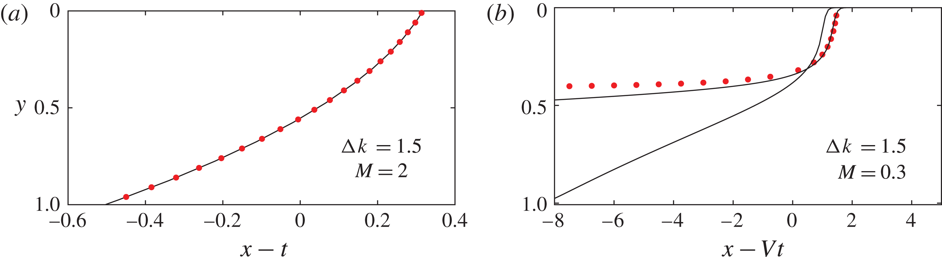
Shocks in travelling-wave coordinates. The solid lines are the numerical results and the red dots show the shape predicted by the steady travelling-wave solutions found in §§ 5.2 and 5.3. (a) The full shock from figure 2(c) shown at
 $t=10$
, which has excellent agreement with the asymptotic shape. (b) The partial shock from figure 2(b) shown at
 $t=10$
and
 $t=100$
in coordinates moving at the speed of the shock, given by (5.18). Convergence to the asymptotic shape is much slower for the partial shock.

5.2 Full shock interface
When the parameter values do not satisfy the inequality (5.6), a shock needs to be introduced to solve (5.2). If
 $F^{\prime }(h)$
is monotonically increasing in
 $(0,1)$
, then all the characteristics of the advection equation (5.2), given by (5.4), cross and a weak solution (with a discontinuity) can be sought; the solution develops a shock that extends across the whole aquifer from
 $h=0$
to
 $h=1$
. The shock requires
 $F^{\prime \prime }(h)$
(5.5) to be positive in
 $(0,1)$
. For the linear variation of permeability (3.1), the condition for the full shock in terms of the parameters is
 $$\begin{eqnarray}\displaystyle & \displaystyle M\geqslant {\displaystyle \frac{1}{1+\unicode[STIX]{x0394}k/2}}. & \displaystyle\end{eqnarray}$$
In the absence of gravity, this shock would not occur; instead, the buoyant injectate would be driven along the base of the aquifer by the combination of higher permeability and the low viscosity of the ambient fluid. Buoyancy forces balance this effect and so the light injectate rises to the top of the aquifer and the interface travels with constant shape and velocity. Mass conservation implies the shock travels with unit velocity (see figure 2 c).
The numerical results in travelling coordinates, shown in figure 5(a), can be used to inspect the approximately vertical interface in figure 2(b). The shock is not in fact a zero-width vertical line; it is smoothed by the buoyancy force. We seek to find the shape of this non-vertical shock.
For parameter values such that the full shock condition given by (5.9) is satisfied, the interface moves with unit velocity, and this motivates our seeking a travelling-wave solution to the full equation (2.16), with
 $h(x,t)=h(\unicode[STIX]{x1D702})$
where
 $\unicode[STIX]{x1D702}=x-t$
. Dropping the time derivative and integrating, we find that the shape satisfies
 $$\begin{eqnarray}\displaystyle & \displaystyle h=1,\quad \unicode[STIX]{x1D702}\leqslant \unicode[STIX]{x1D702}_{1}, & \displaystyle\end{eqnarray}$$
 $$\begin{eqnarray}\displaystyle & \displaystyle {\displaystyle \frac{\text{d}h}{\text{d}\unicode[STIX]{x1D702}}}={\displaystyle \frac{K(h)-Mh+(M-1)hK(h)}{MK(h)(1-K(h))}},\quad \unicode[STIX]{x1D702}_{1}<\unicode[STIX]{x1D702}<\unicode[STIX]{x1D702}_{0}, & \displaystyle\end{eqnarray}$$
 $$\begin{eqnarray}\displaystyle & \displaystyle h=0,\quad \unicode[STIX]{x1D702}\geqslant \unicode[STIX]{x1D702}_{0}. & \displaystyle\end{eqnarray}$$
The constant of integration is set to zero because the gradient is finite as
 $h\rightarrow 0$
. The contact points are constants,
 $\unicode[STIX]{x1D702}_{0}=x_{0}(t)-t$
and
 $\unicode[STIX]{x1D702}_{1}=x_{1}(t)-t$
at the top and base of the aquifer, respectively. Note that
 $\unicode[STIX]{x1D702}_{1}<0$
and
 $\unicode[STIX]{x1D702}_{0}>0$
. The separation of the contact points can be found by numerically integrating equation (5.11) across the aquifer:
 $$\begin{eqnarray}\displaystyle \unicode[STIX]{x1D702}_{0}-\unicode[STIX]{x1D702}_{1}=\int _{h=1}^{h=0}\left({\displaystyle \frac{\text{d}h}{\text{d}\unicode[STIX]{x1D702}}}\right)^{-1}\text{d}h. & & \displaystyle\end{eqnarray}$$
The shape of the travelling-wave interface is independent of the position of the contact points because the right-hand side of (5.11) is independent of
 $\unicode[STIX]{x1D702}$
. We can find the shape by solving (5.11) numerically with an arbitrary choice of
 $\unicode[STIX]{x1D702}_{1}$
. To determine the position of the contact points, we use mass conservation, which is
 $$\begin{eqnarray}\displaystyle \unicode[STIX]{x1D702}_{1}+A=0, & & \displaystyle\end{eqnarray}$$
where
 $A$
is the area under the interface shape in the partially flooded region.
The red dots in figure 5(a) show the travelling-wave solution we have just calculated. There is good agreement with the numerical solution to the full governing equation (2.16) at
 $t=10$
which is plotted as a solid black line.
Our model in § 2 used the hydrostatic pressure assumption and, for this constant wave solution to be consistent, we require that the shape has a shallow gradient so that
 $$\begin{eqnarray}\displaystyle B={\displaystyle \frac{q_{0}}{UH}}\ll 1. & & \displaystyle\end{eqnarray}$$
This is equivalent to requiring that the injection flux is small compared to the natural buoyancy velocity. In contrast to the case of a shock, this condition can be relaxed when the interface spreads as a rarefaction wave since the gradient becomes progressively shallower at late times.
5.3 Compound rarefaction-shock interface
There are regions of
 $(\unicode[STIX]{x0394}k,M)$
parameter space outside that given by the inequalities (5.6) and (5.9) in which
 $F(h)$
is neither concave nor convex. For a linearly varying permeability (3.1),
 $F^{\prime }(h)$
has a single maximum, in
 $(0,1)$
, for those values of
 $M$
and
 $\unicode[STIX]{x0394}k$
. The velocity of the interface is then faster in the middle of the aquifer than at the top and the bottom; the buoyant injectate in the middle would then lie underneath the heavy ambient fluid at the top of the aquifer. We assume that the vertical adjustment due to buoyancy and Rayleigh–Taylor fingering is much faster than the along-channel advection of fluid driven by injection (see Huppert, Neufeld & Strandkvist Reference Huppert, Neufeld and Strandkvist2013). In this limit, we expect a compound solution: a rarefaction wave in
 $h_{s}<h<1$
and a vertical shock across
 $0<h<h_{s}$
, where
 $h_{s}$
is the height of the shock (see figure 2
b).
The partial shock travels with a velocity of at least 1 owing to mass conservation. In the region of parameter space outside the full shock region, the velocity of the trailing contact point
 $M(1+\unicode[STIX]{x0394}k/2)$
is less than 1 (see (5.9)) and hence travels slower than the partial shock. This confirms that, when
 $F^{\prime }(h)$
has a single maximum in
 $(0,1)$
, the shock does not occupy the entire depth of the aquifer.
Assuming the partial shock is approximately vertical at late times, mass conservation implies that the speed
 $V$
of the shock satisfies
 $$\begin{eqnarray}\displaystyle Vh_{s}={\displaystyle \frac{K(h_{s})}{M+(1-M)K(h_{s})}}, & & \displaystyle\end{eqnarray}$$
which is equivalent to a Rankine–Hugoniot condition. The physical requirement that the interface must be continuous at the contact point between the wave and the shock imposes
 $$\begin{eqnarray}\displaystyle V=F^{\prime }(h_{s}). & & \displaystyle\end{eqnarray}$$
For a linear
 $k(y)$
, equations (5.16) and (5.17) can be solved for
 $V$
and
 $h_{s}$
to give
 $$\begin{eqnarray}\displaystyle h_{s}=1-{\displaystyle \frac{2}{\unicode[STIX]{x0394}k}}\pm \sqrt{{\displaystyle \frac{2M}{(1-M)\unicode[STIX]{x0394}k}}},\quad V={\displaystyle \frac{1}{\bigg(1-M\bigg)\bigg(1-{\displaystyle \frac{2}{\unicode[STIX]{x0394}k}}\pm 2\sqrt{{\displaystyle \frac{2M}{(1-M)\unicode[STIX]{x0394}k}}}\bigg)}}, & & \displaystyle \nonumber\\ \displaystyle & & \displaystyle\end{eqnarray}$$
where the positive square root is taken in
 $M<1,~\unicode[STIX]{x0394}k>0$
(II in figure 4) and the negative root in
 $M>1,~\unicode[STIX]{x0394}k<0$
(II
 $^{\prime }$
in figure 4). There are no solutions in the other two quadrants, as a compound solution is not possible there. Although II and II
 $^{\prime }$
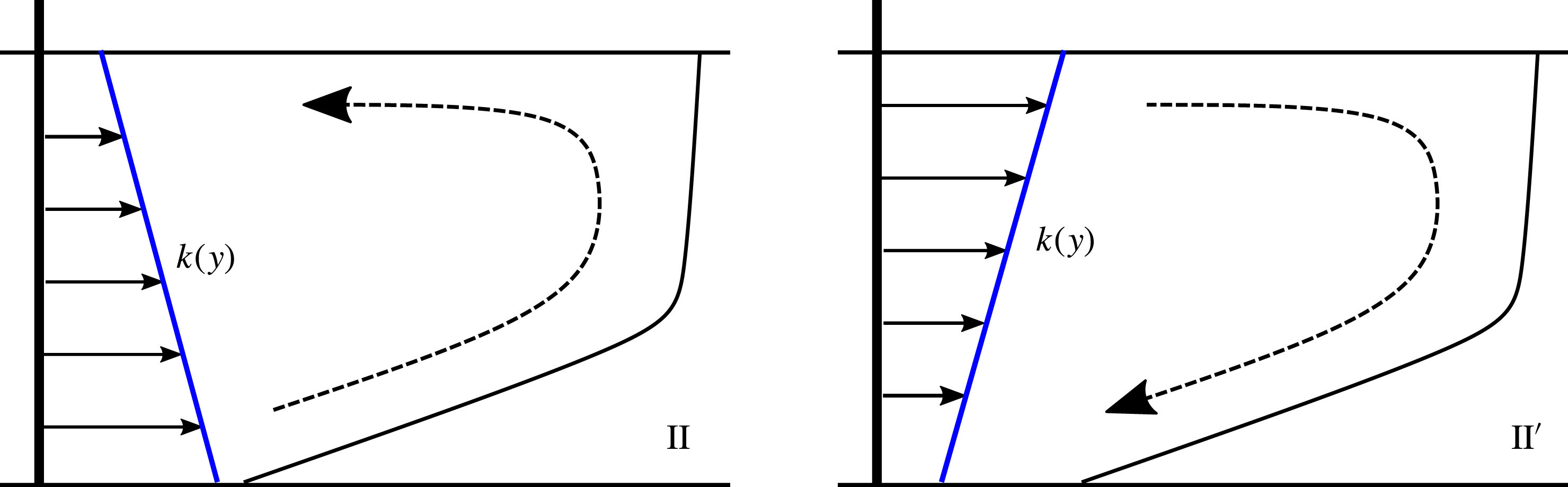
both give rise to compound interface shapes, the flows are physically different, as shown in figure 6. In II, the buoyant injectate migrates along the high-permeability region at the base of the aquifer and then rises in the growing nose into the low-permeability region, but the interface advances more rapidly in this upper region of the system. In II
 $^{\prime }$
,
 $\unicode[STIX]{x0394}k<0$
and the fluid at the top of the aquifer catches the front and is deflected down into the low-permeability region.
The two different flow structures in a compound rarefaction–shock interface. For parameters in region II (
 $\unicode[STIX]{x0394}k>0$
), the shock is at the base of the shear; whilst in region II
 $^{\prime }$
(
 $\unicode[STIX]{x0394}k<0$
), the shock is at the top of the shear. The dashed line shows how fluid enters and then exits the nose region in each regime.

As with the full shock, we expect the shape of the partial shock not to be a zero-width vertical line because buoyancy smoothes the interface. We adopt a similar approach to that of § 5.2 to find the structure of the partial shock. The shock moves with speed
 $V$
, and to capture its dynamics we seek a travelling-wave solution in the shock region (
 $h<h_{s}$
). In the rarefaction region (
 $h>h_{s}$
), the interface has gradient of order
 $t^{-1}$
. Assuming we are at long times, we impose the boundary condition
 $\text{d}h/\text{d}\unicode[STIX]{x1D702}\rightarrow 0$
, as
 $h\rightarrow h_{s}$
, on the shape of the shock. We transform the full governing equation (2.16) using the travelling coordinate
 $\unicode[STIX]{x1D702}=x-Vt$
. We drop the time derivative and integrate to find
 $$\begin{eqnarray}\displaystyle & \displaystyle {\displaystyle \frac{\text{d}h}{\text{d}\unicode[STIX]{x1D702}}}={\displaystyle \frac{K(h)-Vh[K(h)+M(1-K(h))]}{MK(h)(1-K(h))}}\quad \text{in}~h<h_{s}, & \displaystyle\end{eqnarray}$$
where the constant of integration is set to zero to satisfy the condition of zero gradient at
 $h=h_{s}$
. The matching with the rarefaction region leads to the shape having an infinite horizontal extent in the
 $\unicode[STIX]{x1D702}$
coordinates, and the position of the leading contact point cannot be determined using mass conservation.
Instead, we solve (5.19) numerically with initial condition
 $h(0)=0$
and then translate the solution to fit the full numerical solution at some late time. Figure 5(b) shows the
 $t=100$
interface as a black line, and the shape given by (5.19) as red dots. In figure 5(a), the asymptotic shape is compared to the
 $t=10$
interface. We include the
 $t=10$
interface in figure 5(b) to illustrate that convergence to the full shock shape is much faster than convergence to the partial shock shape. Unlike the full shock shape, the partial shock shape (5.19) is only valid in the limit as
 $t\rightarrow \infty$
. This is because we imposed that the gradient at
 $h=h_{s}$
must be zero but the gradient of the rarefaction is
 $O(t^{-1})$
at
 $h=h_{s}$
.
5.4 Singular solution for
 $\unicode[STIX]{x0394}k=0$
,
$M=1$


We have found three different late-time regimes and the values of the viscosity ratio and permeability difference for which they occur (see figure 4). The four regions I, II, II
 $^{\prime }$
and III touch at the point
 $\unicode[STIX]{x0394}k=0$
,
 $M=1$
. The late-time solutions for this special case of injection of an equal viscosity fluid into a uniform aquifer were found by Huppert & Woods (Reference Huppert and Woods1995). The distance between the injection well and the fluid–fluid interface is proportional to
 $t$
and the extent of the front grows proportional to
 $t^{1/2}$
(see figure 2
d), an altogether different result from those found for regions I, II, II
 $^{\prime }$
and III. This is a singular solution, since, if the aquifer is not uniform or the viscosity ratio is not exactly 1, it is invalid. In that case, the late-time regime will move to one of the cases described above.
6 Multiple shock solutions
Thus far in this paper we have restricted our attention to aquifers where the permeability increases or decreases linearly from top to bottom. Reservoir rock is typically more complicated than this. Permeabilities can vary significantly over small vertical distances and we expect that there may be more complex late-time regimes as well as the three described earlier for the relatively simple linear vertical variations in permeability. It is possible to have two or more separate shocks across the aquifer moving at different speeds. In the analogous problem of viscous channel flow, a double shock has been observed (see Taghavi et al.
Reference Taghavi, Seon, Martinez and Frigaard2009) but not in a porous medium. This can have significant implications for reservoir sweep, which is important in both enhanced oil recovery and geologic
 $\text{CO}_{2}$
sequestration. In this section, to demonstrate the phenomenon, we consider a more complex cross-layer permeability in which there is a local minimum and local maximum of the permeability within the layer:
 $$\begin{eqnarray}\displaystyle k(y)=1+15(y-1)(y-{\textstyle \frac{1}{2}})y. & & \displaystyle\end{eqnarray}$$
For simplicity, we take
 $M=1$
so that the advection speeds of constant
 $h$
are given by
 $$\begin{eqnarray}\displaystyle {\displaystyle \frac{\text{d}x}{\text{d}t}}=F^{\prime }(h)=k(h). & & \displaystyle\end{eqnarray}$$
Since there is a local minimum
 $h_{-}$
and a local maximum
 $h_{+}$
in the permeability with
 $h_{-}>h_{+}$
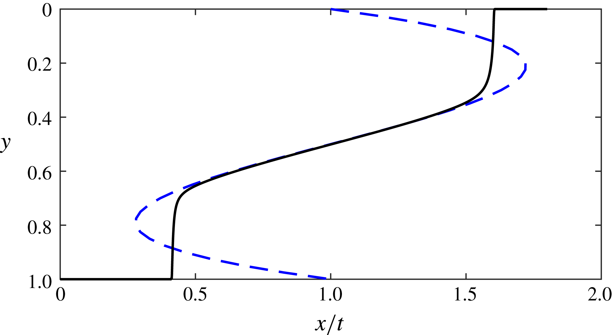
, two shock-like regions develop (see figure 7).
Interface shape for a double shock (solid black line) at
 $t=100$
. The governing equation has been solved numerically for
 $k(y)$
given by (6.1). The blue dashed line illustrates how the permeability varies with height and gives the characteristic speeds
 $F^{\prime }(h)=k(h)$
for the advection equation.

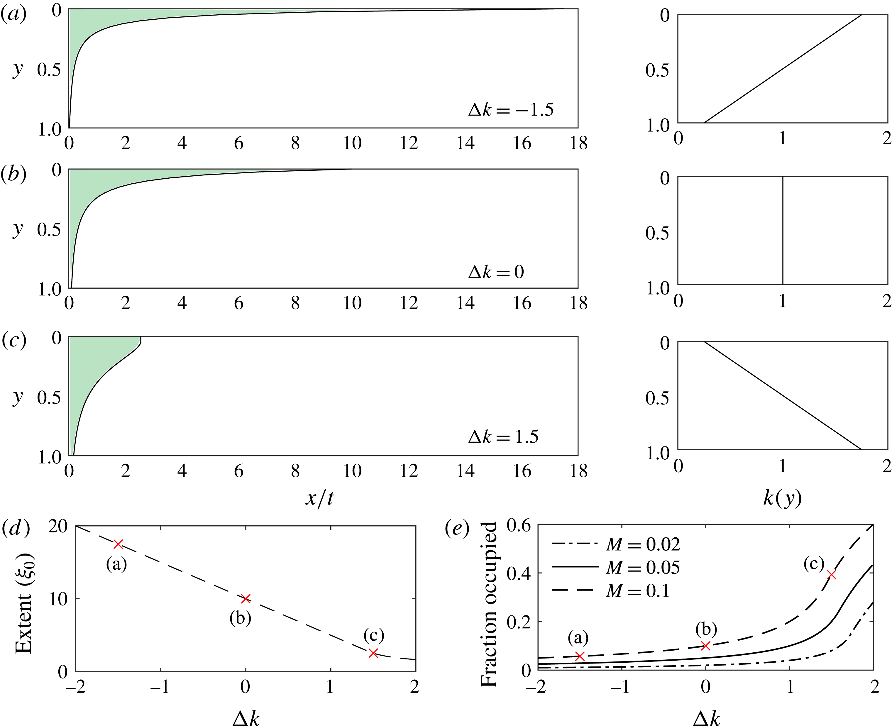
(a–c) Shape of the interface in
 $x/t$
coordinates for
 $M=0.1$
and three different permeability gradients, which are shown in the right-hand column. (d) The position of the leading contact point as a function of
 $\unicode[STIX]{x0394}k$
for
 $M=0.1$
. (e) The fraction of pore space occupied as a function of the permeability gradient for three values of the viscosity ratio typical in carbon sequestration. The red crosses correspond to the interfaces in (a), (b) and (c) showing how a steeper interface leads to a greater fraction of pore space invaded.

7 Implications for
$\text{CO}_{2}$
sequestration

When using geologic formations as a means of storing
 $\text{CO}_{2}$
, it is important to have accurate estimates of the fraction of the pore space into which
 $\text{CO}_{2}$
can be stored. In particular, the critical volume fraction of interest corresponds to the fraction of pore space accessed by the
 $\text{CO}_{2}$
between the injection well and the leading contact point of the
 $\text{CO}_{2}$
plume (Celia et al.
Reference Celia, Bachu, Nordbotten and Bandilla2015). This is because, once the leading edge of the plume reaches a particular distance from the injection well, the injection may need to cease, either for reasons of security of storage if there are faults or fractures downstream of the injection well, or, in a commercial setting, if different organisations have rights to
 $\text{CO}_{2}$
sequestration in adjacent regions of land. The fraction of the pore space accessed by the
 $\text{CO}_{2}$
plume during the injection phase will represent the maximum fraction of the pore space into which the
 $\text{CO}_{2}$
can be sequestered, since the subsequent motion of the
 $\text{CO}_{2}$
is controlled by buoyancy, and hence the plume will subsequently tend to thin and spread. The impact of the plume structure and shape is therefore key for estimating the efficiency of the sequestration (Bachu Reference Bachu2015).
In this paper we have shown that the presence of a vertical permeability gradient across an aquifer plays a key role in the dynamics of the interface. Here we apply our results to illustrate how such a permeability gradient influences the fraction of pore space accessed by the
 $\text{CO}_{2}$
.
We define the available pore space as the product of the position of the leading contact point and the depth of the aquifer. The position of the leading contact point in the
 $\unicode[STIX]{x1D709}=x/t$
coordinates predicted by the long-time asymptotic solutions is a constant,
 $\unicode[STIX]{x1D709}_{0}=x_{0}(t)/t$
. The area invaded equals the amount of fluid injected, which, in dimensionless variables, is
 $t$
. The fraction of pore space invaded is the ratio of these two quantities:
 $$\begin{eqnarray}\displaystyle {\displaystyle \frac{t}{x_{0}(t)}}={\displaystyle \frac{1}{\unicode[STIX]{x1D709}_{0}}}. & & \displaystyle\end{eqnarray}$$
This implies that the fraction of the pore space invaded is independent of time, as found by Guo et al. (Reference Guo, Zheng, Bandilla, Celia and Stone2016b ) for a radial, vertically homogeneous aquifer. Unlike the radial case, however, the fraction invaded is independent of the buoyancy parameter (2.17) because at late times the role of buoyancy can be neglected.
Supercritical carbon dioxide is typically much less viscous than the ambient brine in storage sites and we take the values
 $M=0.1$
,
 $0.05$
and
 $0.02$
in our examples, since
 $M$
varies with the depth of the aquifer. In the classical model with
 $\unicode[STIX]{x0394}k=0$
, these choices of
 $M$
lead to the interface following the shape of a rarefaction wave with the injectate migrating fastest at the top of the aquifer. For
 $\unicode[STIX]{x0394}k<0$
, the
 $\text{CO}_{2}$
migrates even faster at the top of the aquifer owing to the relatively high permeability there, causing the rarefaction to be elongated and the fraction of pore space invaded to be reduced. Conversely, for
 $\unicode[STIX]{x0394}k>0$
, the interface is steeper and the pore space occupied is greater. The interfaces for these three cases are shown in figure 8 for
 $M=0.1$
and
 $\unicode[STIX]{x0394}k=0,~\pm 1.5$
. The right-hand column of figure 8 shows the associated permeability profiles. For sufficiently large
 $\unicode[STIX]{x0394}k$
, the parameters move from region I into region II in figure 4 and there is a shock at the top of the aquifer, which alters the fraction stored (see figure 8
c). The fraction occupied for each of our parameter choices is labelled (a), (b) and (c) in figure 8(e), which illustrates how the fraction of pore space occupied depends on
 $\unicode[STIX]{x0394}k$
for our three choices of
 $M$
.
It is clear that the fraction of pore space invaded is highly dependent on the permeability profile; for example, when
 $M=0.1$
, in an aquifer with
 $\unicode[STIX]{x0394}k=1.5$
, the
 $\text{CO}_{2}$
invades approximately four times the pore space invaded in a uniform aquifer of the same mean permeability. For reference,
 $\unicode[STIX]{x0394}k=1.5$
represents an aquifer in which the permeability varies by a factor of 7. Using the Kozeny–Carman relation that suggests the permeability is proportional to the grain size squared,
 $\unicode[STIX]{x0394}k=1.5$
only requires the grain size to vary by a factor of
 $2.65$
across the aquifer, which is within measured values for many aquifers (Carman Reference Carman1939). Therefore, in making storage estimates there is an important uncertainty associated with vertical heterogeneities. Our results could be applied to find the probability distribution of the fraction of pore space occupied given a large dataset of permeability variations in aquifers.
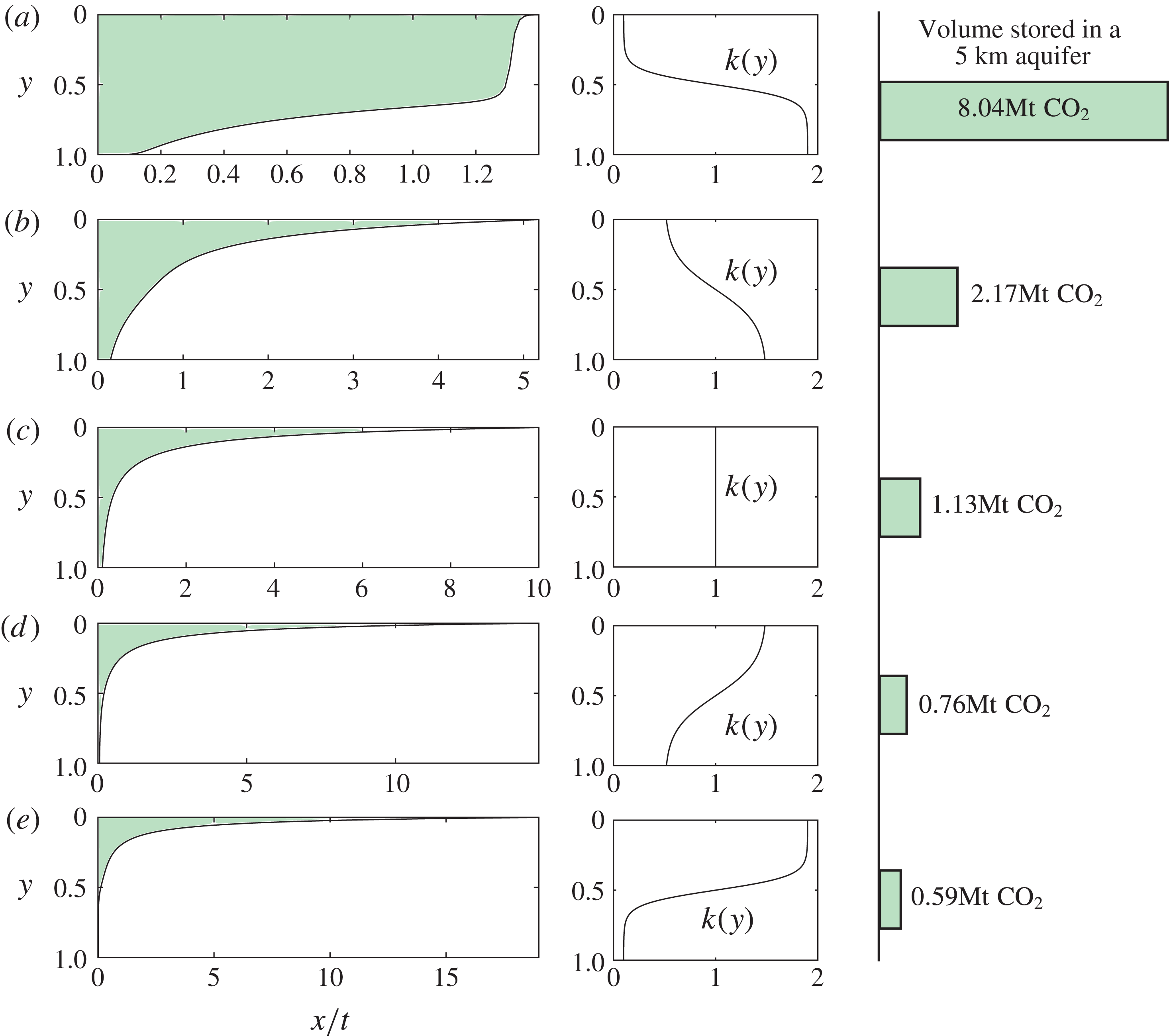
Interface shapes and volume of
 $\text{CO}_{2}$
stored for nonlinear permeability profiles including lenses of high and low permeability. The first column shows the interface shape in
 $x/t$
coordinates, and the corresponding permeability profile is shown in the second column. We calculate the volume of
 $\text{CO}_{2}$
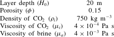
stored for each permeability profile in an aquifer which is 20 m deep and 1000 m wide, assuming injection must stop when the leading edge of the plume has travelled 5000 m from the injection well. The parameter values are given in table 1. The location of the high- and low-permeability lenses has a significant influence on the volume stored.

7.1
$\text{CO}_{2}$
storage in a real aquifer with lenses of high and low permeability

In this subsection, we extend the analysis above to the case of a nonlinear permeability profile and we calculate how the permeability structure influences the volume of
 $\text{CO}_{2}$
stored in a typical project. We compare permeability profiles, each with the same mean permeability, in which there are lenses of high and low permeability. These profiles are shown in figure 9, where the left-hand column shows the interface shape. We assume that the aquifer and the injection well are 1 km wide (in the direction out of the plane in figure 9). We can calculate the mass of
 $\text{CO}_{2}$
stored using the parameter values in table 1. We assume injection is required to stop when the plume reaches a point 5 km from the injection well. These volumes are shown in figure 9 and demonstrate that the volume of
 $\text{CO}_{2}$
stored is heavily dependent on the location of the low- and high-permeability lenses.
Parameter values for a typical aquifer.

8 Conclusion
In this contribution we have analysed the injection of buoyant fluid into an aquifer where the permeability varies vertically. With a permeability that varies linearly with height, we have found four late-time regimes, including a compound rarefaction–shock interface which does not occur in a uniform porous medium. Our parameter space shows that the classic solution for equally viscous fluids in a uniform aquifer is singular and unstable to small changes in the permeability profile. Applying our results to the problem of carbon storage, we have shown that cross-aquifer permeability differences can significantly influence the volume of
 $\text{CO}_{2}$
that can be stored in an aquifer. When the assumption of permeability that varies only linearly with height is relaxed, we have found that it is possible to have two separate shocks that travel at different speeds in a porous medium. Our study has shown that the early time period is dependent not only on the viscosity ratio but also on the permeability at the top of the aquifer.
Acknowledgements
The authors wish to thank T. Espie for his support of this work, and BP and EPSRC for the award of a CASE studentship funding the research.