





1. Introduction
Large language models (LLM) are rapidly becoming a default “second opinion” for everyday economic decisions: from buying insurance to interpreting probabilistic information in medical settings. Investors are also increasingly relying on robo-advisors for portfolio decisions, with the market projected to reach \$33.38 billion by 2030.Footnote 1 As LLM-based recommendations diffuse into daily life, a central question for economics has been raised: how do LLM-based recommendations reshape decision making under uncertainty, and how do they affect risk and ambiguity attitudes, which are key measures for economic modeling?
Our experiments introduce standard, incentivized valuation tasks where individuals state their certainty equivalents for risky and ambiguous lotteries while receiving (or not receiving) an LLM-based recommendation. We also manipulate the complexity of the evaluated lotteries using compound lotteries where deriving the objective reduced-form probabilities might be cognitively costly. Our design links two literatures: attitudes toward risk, ambiguity, and complexity, and how decision makers incorporate recommendations into their choices. We show that LLM-based recommendations shift value distributions and reduce variations in them. This result is robust across environments that vary in uncertainty and cognitive complexity, suggesting that LLM-based recommendations may attenuate behaviors driven by extreme risk and ambiguity attitudes.
Our baseline design follows standard preference-elicitation practice using a standard multiple price list method, and the tasks are based on de Clippel et al. (Reference de Clippel, Moscariello, Ortoleva and Rozen2024). Participants value four prospects that pay \$30 if a “purple” card is drawn from a described deck and \$0 otherwise: (i) a transparent 50/50 lottery; (ii) a compound lottery with two underlying decks that reduces to 50/50; (iii) a more complex compound lottery with four underlying decks that also reduces to 50/50; and (iv) an ambiguous lottery in which the deck composition is unknown. This design varies the informational and computational demands of evaluation while holding fixed the reduced-form probability of winning. Our main intervention randomizes access to LLM-based recommendation generated by ChatGPT (GPT-4o), we call this “AI treatment”. To standardize informational content and rule out a possible impact caused by endogenous prompting, all participants in the AI treatment view the same pre-generated screenshots for each lottery. The Baseline treatment asks participants to perform the same tasks without LLM-based recommendation.
LLM-based recommendations have economically meaningful effects on valuations in our data, but not through the mean. Across all four lotteries, average certainty equivalents are statistically indistinguishable in the Baseline and AI treatments. Instead, the entire distribution shifts: certainty equivalents in AI treatment exhibit second-order stochastic dominance relative to the Baseline treatment. In practical terms, LLM-based recommendations leave mean valuations unchanged while compressing dispersion and hence, reducing heterogeneity. After each compound lottery, we also elicit beliefs about the probability of winning the prize and ask participants how certain they feel about those beliefs. Without LLM-based recommendations, participants are more likely to form incorrect beliefs about their chances of winning in the more complex lottery than in the less complex one. Specifically, their beliefs are more likely to deviate from the 50/50 benchmark in the more complex setting. However, this gap disappears when LLM-based recommendations are provided. We further show that, among participants classified as complexity averse, lower cognitive uncertainty is associated with a smaller magnitude of complexity aversion. Hence, a natural interpretation is that LLM-based recommendations compress valuations by reducing cognitive uncertainty, consistent with Enke and Graeber (Reference Enke and Graeber2023). Additionally, while LLM-based recommendations shift the intensity of risk, complexity, and ambiguity aversion, they do not affect the fractions of participants classified as averse, neutral, or loving.
Motivated by the evidence that people seek expert advice more when the situation is complex, and uncertainty is enhanced, Engelmann et al. (Reference Engelmann, Capra, Noussair and Berns2009) use fMRI scanning of the participants and show that expert advice corrects understanding of probabilities through “offloading” the calculation burden. While this particular study did not vary the level of difficulty or complexity of the uncertainty the decision makers evaluate, the mechanism identified might be particularly relevant in complex environments where computation is costly and where recommendations may affect confidence and perceived understanding rather than correcting probabilistic reasoning. Related to this intuition, de Clippel et al. (Reference de Clippel, Moscariello, Ortoleva and Rozen2024) showed that individuals value risk less when they perceive a lottery as complex and ambiguous. Building on these findings, our design can address whether the impact of LLM-based recommendations is robust to variation in the complexity of uncertainty involved.
We also contribute to the recommendation literature. Previous work shows that recommendations, in the form of direct human advice and broader social interactions, systematically shape economic choice. {The social psychology literature on advice taking identifies environmental complexity, uncertainty, and decision-maker confidence as some of the key determinants of whether advice is followed or ignored (see Bonaccio & Dalal, Reference Bonaccio and Dalal2006; Kämmer et al., Reference Kämmer, Choshen-Hillel, Müller-Trede, Black and Weibler2023; and Rader et al., Reference Rader, Larrick and Soll2017, for surveys). The Judge-Advisor System is a well-established paradigm in this literature for studying how individuals seek, evaluate, and use advice. Our subjective lottery-evaluation setting differs from the Judge-Advisor System in which participants typically infer an objectively true outcome from provided information. Because individuals differ in their risk tolerance, there is no objectively correct answer in our context. Nevertheless, this literature is useful for motivating several aspects of our design and for guiding future research on advice in personal risk evaluation. Rebholz and Hütter (Reference Rebholz and Hütter2022) show that advice receives greater weight if it is expected, so because our instructions tell subjects that recommendations will be provided, we do not expect them to ignore the LLM-based recommendations. In addition, the LLM-based value recommendations in our experiments include detailed explanations of the expected value of the lotteries and of how evaluations of the subjects should relate to their risk and ambiguity tolerance. Based on Rebholz et al. (Reference Rebholz, Koop and Hütter2024), which shows that explanation availability increases advice uptake in the Judge-Advisor System, we expect the detailed content of the LLM-based recommendations to have a significant effect in our experiments.
In laboratory settings, consultation with others compresses dispersion in risk taking (Bougheas et al., Reference Bougheas, Nieboer and Sefton2013), observing a peer take a risky action increases risk taking (Cooper & Rege, Reference Cooper and Rege2011), and group decision making can reduce ambiguity sensitivity relative to individual choice (Keck et al., Reference Keck, Diecidue and Budescu2014). In financial contexts, social interactions affect retirement plans (Duflo & Saez, Reference Duflo and Saez2003; Beshears et al., Reference Beshears, Choi, Laibson, Madrian and Milkman2015), and field evidence highlights the role of social learning in portfolio and asset choice (Bursztyn et al., Reference Bursztyn, Ederer, Ferman and Yuchtman2014). Related work in strategic environments also documents sizable effects of advice in settings such as ultimatum and coordination games (Schotter, Reference Schotter2003; Çelen et al., Reference Celen, Kariv and Schotter2010). Our study builds on these insights: external guidance can change the distribution of choices.
More recently, attention has shifted from human recommendations to algorithmic AI recommendations, and to natural-language AI recommendations in the early 2020s.Footnote 2 Evidence from large-scale experiments suggests that robo-advisors can reduce investor mistakes (Lambrecht et al., Reference Lambrecht, Oechssler and Weidenholzer2024), shift the focus of human investors to sectors where they have advantages over AI (Raymond, Reference Raymond2024), and reduce child hospitalization when the child protective services receive risk scores from algorithms (Grimon & Mills, Reference Grimon and Mills2025). However, the results are mixed in different settings, as Kreitmeir & Raschky (Reference Kreitmeir and Raschky2024) showed that better programmers achieve worse outputs when AI assistance is allowed, highlighting an important tension between algorithm aversion (Dietvorst et al., Reference Dietvorst, Simmons and Massey2015) and algorithm appreciation (Logg et al., Reference Logg, Minson and Moore2019). Rebholz et al. (Reference Rebholz, Koop and Hütter2024) show that both explanation availability and the ability to engage with the AI increase advice uptake independently in the Judge-Advisor System, while there is no evidence that advice weighting differs depending on whether explanations are provided versus requested. Complementary work shows that algorithmic advice may mitigate behavioral biases such as the disposition effect and trend chasing (D’Acunto et al., Reference D’Acunto, Prabhala and Rossi2019), or introduce new biases such as psychological cost of being wrong (Almog et al., Reference Almog, Gauriot, Page and Martin2025). On the theory side, models have begun to formalize how recommendations can enter preferences generating over-responsiveness to recommendations (McLaughlin & Spiess, Reference McLaughlin and Spiess2022).
We contribute to this recent literature by asking a basic question: how do LLM-based recommendations affect measured risk, complexity, and ambiguity attitudes in an environment free from social or strategic interactions, and does it shift valuations in one direction or reshape the distribution of valuations across individuals? Moreover, our decision environment should be minimally impacted by some of the behavioral concerns highlighted by the previous research, such as shame, pride, social image, or confidence, as there is no right or wrong answer in valuing a lottery. Since LLM-based recommendations in decision making are here to stay, understanding their impact on risky choice is central for economic modeling.
2. Experiment design
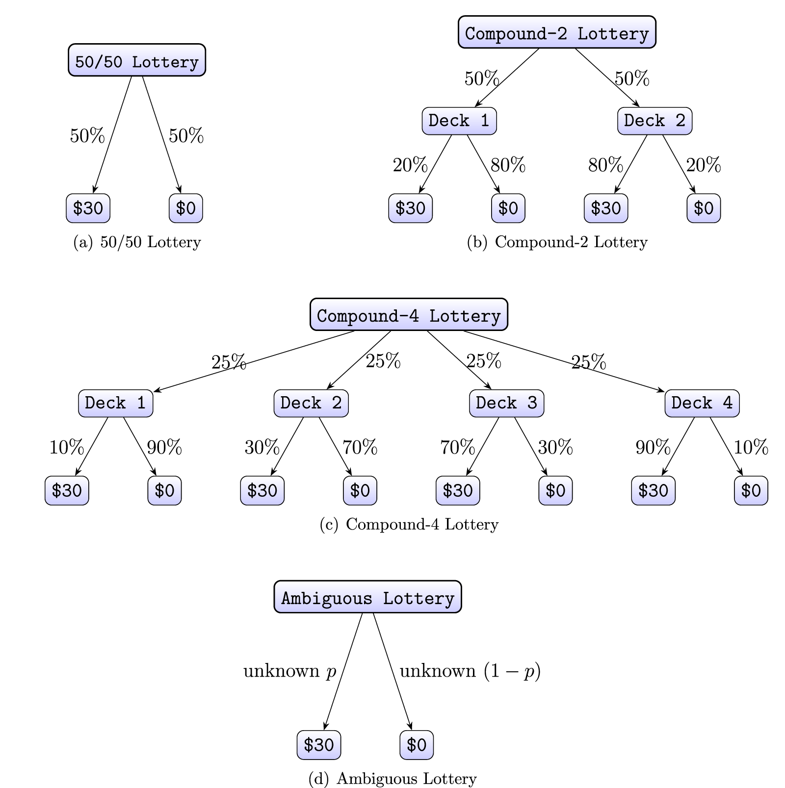
In the experiment, we measure the dollar value that participants assign to multiple lotteries. In each lottery, the computer simulates the draw of a card from a deck of green and purple cards. The bet pays \$30 if the drawn card is purple, and \$0 otherwise. This setting is used in de Clippel et al. (Reference de Clippel, Moscariello, Ortoleva and Rozen2024). We elicit participants’ certainty equivalents for four lotteries using the standard multiple price list (MPL) procedure with enforced single switching (Andersen et al., Reference Andersen, Harrison, Lau and Rutström2006; Holt & Laury, Reference Holt and Laury2002). The MPL varies the sure amounts from \$1 to \$30 with an increment of \$1 at each row. Participants face several scenarios that differ in the complexity of the lotteries (for a graphical interpretation of the below lotteries see Figure 1):Footnote 3
• 50/50 Lottery: The deck contains 50 purple and 50 green cards, making it easy to see that the probability of winning is 50%.
• Compound Lottery, Two Decks (Compound-2): There are two decks of cards, each of which contains 100 purple or green cards. While 20% of the cards are Purple in the first deck, the percentage of the Purple cards is 80% in the second deck. Participants are told that the computer selects one of the two decks at random with equal chance, shuffles the selected deck, and draws a card. Hence, this scenario describes a non-degenerate compound lottery that reduces to a 50/50 probability of drawing a purple card.
• Compound Lottery, Four Decks (Compound-4): There are four decks of cards, each of which contains 100 purple or green cards. The respective percentage of purple cards in each deck is 10%, 30%, 70%, and 90%. Participants are told that the computer selects one of the four decks at random with equal chance, shuffles the selected deck, and draws a card. Similar to the previous lottery, this is also a non-degenerate compound lottery that reduces to a 50/50 probability of drawing a purple card.
• Ambiguous Lottery: Participants are only told that the deck contains 100 purple or green cards, but not the exact composition, and that “they could be all Purple, all Green, or any combination.”
The lotteries asked

Fig. 1 Long description
Four lottery scenarios are illustrated. 1. 50/50 Lottery: A single deck with a 50 percent chance of winning 30 dollars and a 50 percent chance of winning 0 dollars. 2. Compound-2 Lottery: Two decks, each selected with a 50 percent probability. Deck 1 offers a 20 percent chance of winning 30 dollars and an 80 percent chance of winning 0 dollars. Deck 2 offers an 80 percent chance of winning 30 dollars and a 20 percent chance of winning 0 dollars. 3. Compound-4 Lottery: Four decks, each selected with a 25 percent probability. Deck 1 offers a 10 percent chance of winning 30 dollars and a 90 percent chance of winning 0 dollars. Deck 2 offers a 30 percent chance of winning 30 dollars and a 70 percent chance of winning 0 dollars. Deck 3 offers a 70 percent chance of winning 30 dollars and a 30 percent chance of winning 0 dollars. Deck 4 offers a 90 percent chance of winning 30 dollars and a 10 percent chance of winning 0 dollars. 4. Ambiguous Lottery: A single deck with unknown probabilities labeled as p and 1 minus p, offering a chance to win either 30 dollars or 0 dollars.
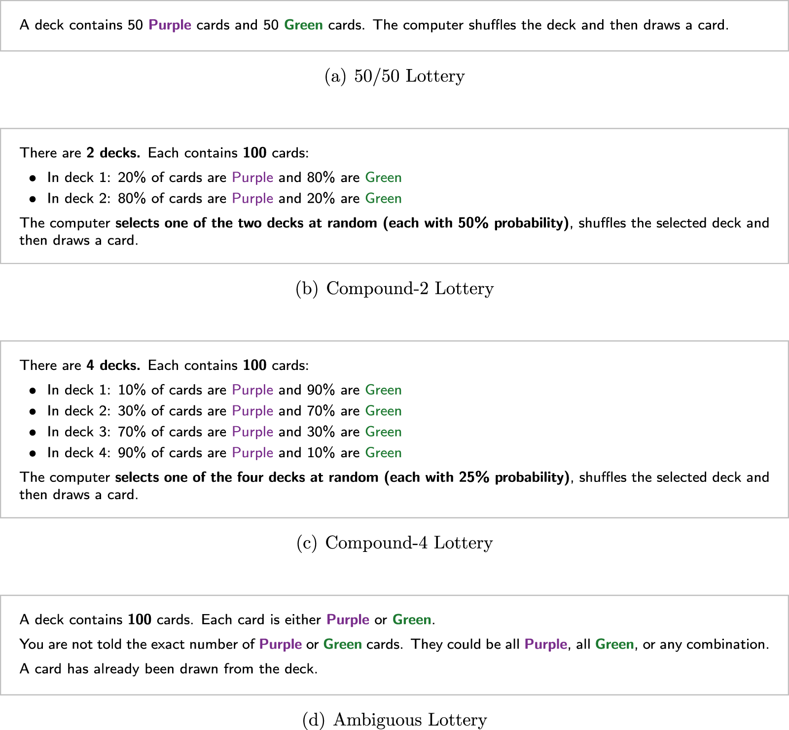
The experiment proceeds as follows. After training about scenarios and MPLs, and after comprehension quizzes, similar to de Clippel et al. (Reference de Clippel, Moscariello, Ortoleva and Rozen2024) participants face a 50/50 lottery, the Compound-2 lottery, the Compound-tfn4 lottery, and, finally, the ambiguous lottery. The information for these lotteries is explained verbally (see Figure 2 for the screenshots used in the experiment). After each compound lottery question, the participants’ belief about drawing a Purple card is elicited in an incentivized way, and they are asked “how certain” they felt about their beliefs.
The scenario of the lotteries

Fig. 2 Long description
A deck contains 50 Purple cards and 50 Green cards. The computer shuffles the deck and then draws a card. There are 2 decks. Each contains 100 cards: In deck 1: 20 percent of cards are Purple and 80 percent are Green In deck 2: 80 percent of cards are Purple and 20 percent are Green The computer selects one of the two decks at random (each with 50 percent probability), shuffles the selected deck and then draws a card. There are 4 decks. Each contains 100 cards: In deck 1: 10 percent of cards are Purple and 90 percent are Green In deck 2: 30 percent of cards are Purple and 70 percent are Green In deck 3: 70 percent of cards are Purple and 30 percent are Green In deck 4: 90 percent of cards are Purple and 10 percent are Green The computer selects one of the four decks at random (each with 25 percent probability), shuffles the selected deck and then draws a card. A deck contains 100 cards. Each card is either Purple or Green. You are not told the exact number of Purple or Green cards. They could be all Purple, all Green, or any combination. A card has already been drawn from the deck.
We randomly assigned participants to either the Baseline or the AI treatment. The Baseline treatment replicates the procedures typically used in the existing literature employing the MPL method in eliciting certainty equivalents of lotteries. In the AI treatment, participants were provided with a lottery-specific recommendation from ChatGPT (Model GPT-4o) before they report their certainty equivalents for each lottery. All participants in the AI treatment were given the same screenshots of recommendations for the corresponding lottery.
Each LLM-based recommendation is generated as follows. Prior to the experiment, we take a screenshot of each lottery exactly as it appears in the Baseline (one lottery at a time), attach the screenshot to ChatGPT, and ask “What do you recommend for someone making these choices?”. Finally, we take screenshots of both our prompt and ChatGPT’s response to this question. We clear ChatGPT’s memory before we inquire about the next lottery. Our design intentionally uses standardized, exogenous advice. For each lottery, we generated the recommendation before the experiment using the same prompt and the corresponding participant-facing lottery screenshot. All participants in the AI treatment then saw the same recommendation for that lottery. This procedure holds fixed the informational content of the recommendation and eliminates endogenous prompting, variation in prompt quality, and variation in follow-up interaction. It therefore allows us to identify the effect of standardized LLM-based recommendations on elicited valuations under uncertainty.
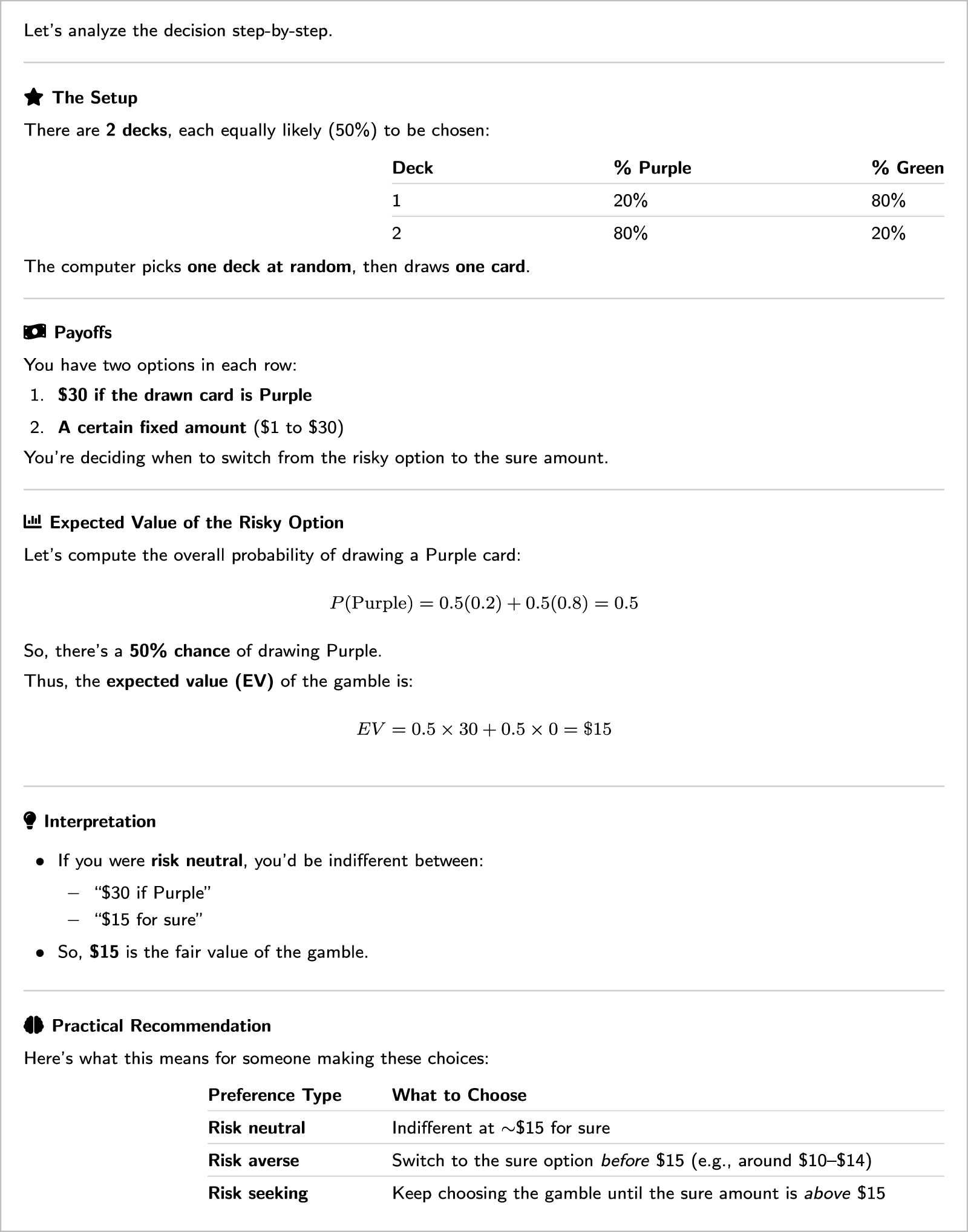
Figure 3 is the LLM-based recommendation for the Compound-2 lottery. Note that it first explains the setup and the task. Then, it explicitly calculates the winning probability and the expected value for this compound lottery. It interprets the expected value as the risk neutral switching point. However, in the practical recommendation it provides a classification of what switching at, before, and after \$15 mean in terms of risk attitudes.
Screenshot of ChatGPT recommendation for the Compound-2 lottery

Fig. 3 Long description
The infographic analyzes a decision step-by-step for a compound lottery. It begins with ′The Setup,′ explaining there are two decks, each equally likely (50 percent) to be chosen. Deck 1 has 20 percent Purple cards and 80 percent Green cards, while Deck 2 has 80 percent Purple cards and 20 percent Green cards. The computer picks one deck at random and then draws one card. ′Payoffs′ section describes two options: 30 dollars if the drawn card is Purple, or a certain fixed amount (1 dollar to 30 dollars). The decision involves choosing when to switch from the risky option to the sure amount. ′Expected Value of the Risky Option′ calculates the overall probability of drawing a Purple card as 0.5, leading to an expected value (EV) of the gamble as 15 dollars. ′Interpretation′ states that if you were risk neutral, you′d be indifferent between 30 dollars if Purple and 15 dollars for sure, making 15 dollars the fair value of the gamble. ′Practical Recommendation′ provides guidance based on preference type: risk neutral individuals are indifferent at approximately 15 dollars for sure, risk averse individuals should switch to the sure option before 15 dollars (around 10 to 14 dollars) and risk seeking individuals should keep choosing the gamble until the sure amount is above 15 dollars.
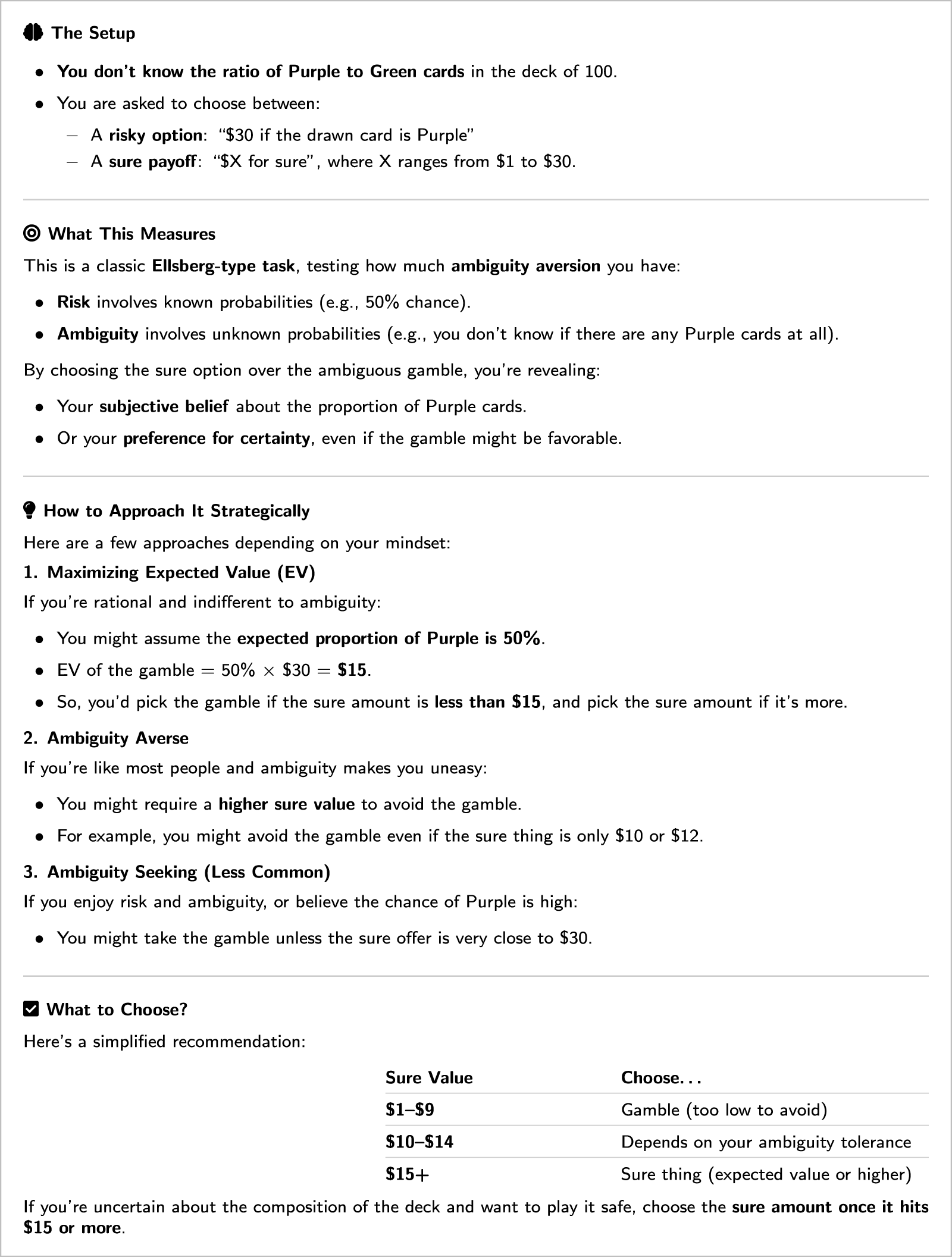
Figure 4 presents the LLM-based recommendation for the ambiguous lottery. As with the risky lotteries, the recommendation includes both technical and practical considerations. It identifies the situation as Ellsberg-type uncertainty and classifies the unknown probabilities as ambiguous. Although it cites \$15 as the expected value under a uniform belief, it emphasizes that the appropriate switching point depends on the decision maker’s tolerance for ambiguity. In Appendix A.1, we provide the screenshots of LLM-based recommendations for all four questions.
Screenshot of ChatGPT recommendation for the ambiguous lottery

Fig. 4 Long description
A formatted instructional handout screenshot with four bold section headings, bullet points and a two-column table at the bottom. The first heading reads ′The Setup′ and states: you don′t know the ratio of Purple to Green cards in the deck of 100. You are asked to choose between a risky option, ′30 dollars if the drawn card is Purple′ and a sure payoff, ′X dollars for sure′, where X ranges from 1 dollar to 30 dollars. The second heading reads ′What This Measures′ and describes the task as a classic Ellsberg-type task testing ambiguity aversion. Two bullet points follow: Risk involves known probabilities (e.g., 50 percent chance). Ambiguity involves unknown probabilities (e.g., you don′t know if there are any Purple cards at all). Two further bullet points state: your subjective belief about the proportion of Purple cards, or your preference for certainty even if the gamble might be favorable. The third heading reads ′How to Approach It Strategically′ with three numbered sub-sections. Sub-section 1, Maximizing Expected Value (EV), lists: you might assume the expected proportion of Purple is 50 percent; EV of the gamble equals 50 percent times 30 dollars equals 15 dollars; so you′d pick the gamble if the sure amount is less than 15 dollars and pick the sure amount if it′s more. Sub-section 2, Ambiguity Averse, lists: you might require a higher sure value to avoid the gamble; you might avoid the gamble even if the sure thing is only 10 dollars or 12 dollars. Sub-section 3, Ambiguity Seeking (Less Common), states: you might take the gamble unless the sure offer is very close to 30 dollars. The fourth heading reads ′What to Choose?′ followed by a two-column table. The left column is headed ′Sure Value′ and the right column is headed ′Choose.′. Row 1: 1 dollar to 9 dollars, Gamble (too low to avoid). Row 2: 10 dollars to 14 dollars, Depends on your ambiguity tolerance. Row 3: 15 dollars plus, Sure thing (expected value or higher). Below the table, bold text states: choose the sure amount once it hits 15 dollars or more.
To check robustness of recommendations with different LLMs, we generated alternative LLM-based recommendations using ChatGPT 5.3, Claude Sonnet 4.6, and Gemini 3.1 Pro (see Appendix A.3).Footnote 4 Both the technical content and the nature of the practical recommendations by all these models were similar. For Q1–Q3, all models explicitly calculate the probability of winning the prize and the expected value of the lotteries, and they explain how risk attitudes should affect the switching point in the list. For Q4, all models refer to Ellsberg-style decision problems and explain how expected value depends on subjective beliefs, together with a recommendation based on the participant’s ambiguity attitude. This robustness in regenerated recommendations confirms that the recommendations used in our experiment are replicable.Footnote 5
We ran the experiment on the Prolific platform in October and November, 2025. The experiment was pre-registered on AsPredicted.org.Footnote 6 Full experimental instructions and screenshots are provided in Appendix A.1. The mean completion time was about 11 minutes. Participants received \$3 for participation, and 10% of participants were eligible for a bonus payment based on their answer to one of the main tasks (drawn at random) following de Clippel et al. (Reference de Clippel, Moscariello, Ortoleva and Rozen2024). The average bonus was \$1.34. In each of the two treatments, there were 300 participants. None of the 600 participants participated in more than one session.
3. Results
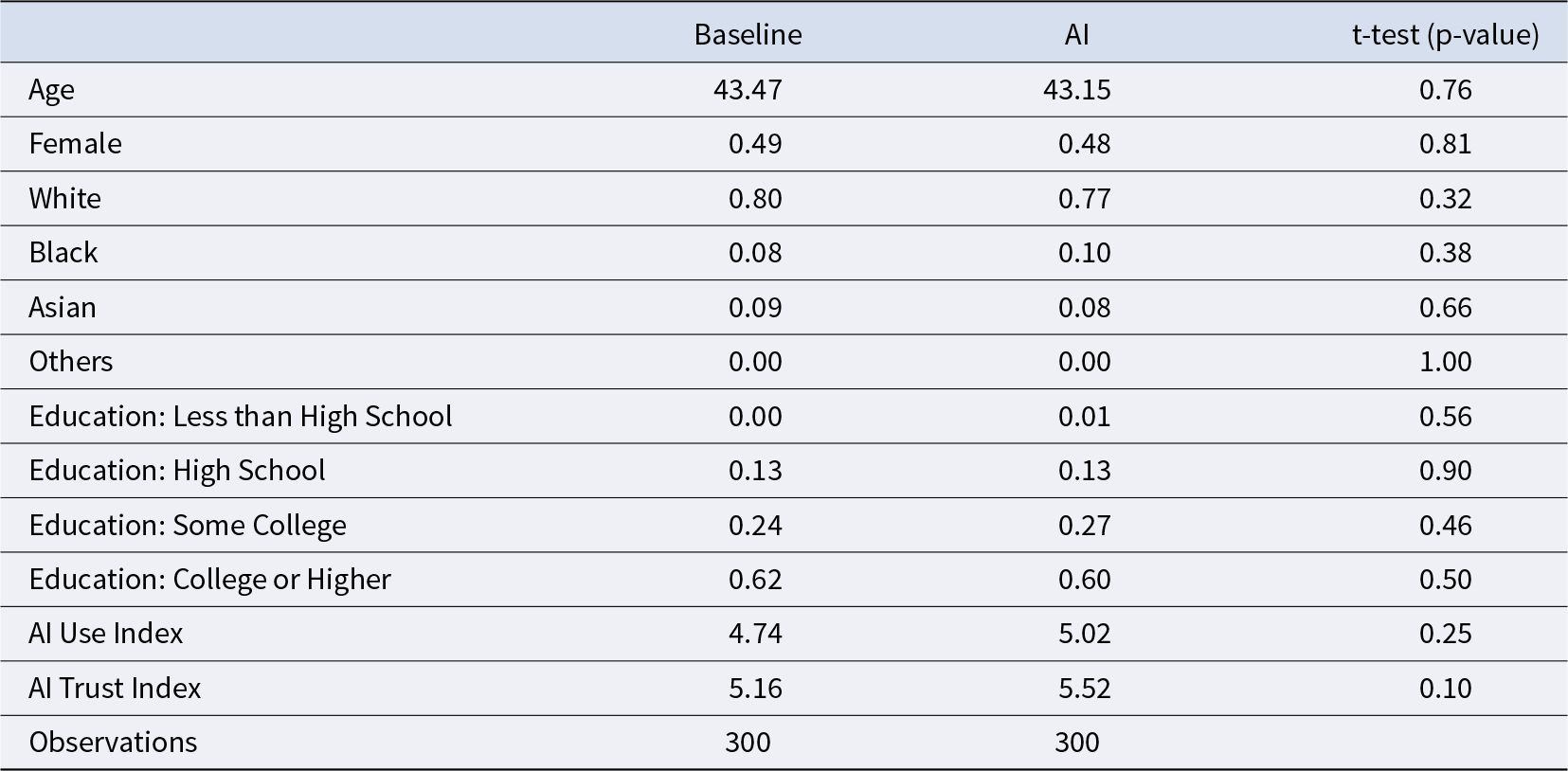
Participants assigned to the Baseline and AI treatments are demographically balanced: gender, race, education distributions and AI use and trust indices are similar across the two treatments (see Table 1). The main body of the paper reports results using all the data. Appendix A.2 repeats the analysis for the participants who pass our comprehension quizzes on the first attempt (82% in the Baseline treatment and 80% in the AI treatment). The results are robust for this filtered subsample.
Demographics

Table 1 Long description
Columns report Baseline, AI, and t-test p-value for each characteristic, with 300 observations in each group. Age is 43.47 in Baseline and 43.15 in AI, with p-value 0.76. Female is 0.49 in Baseline and 0.48 in AI, with p-value 0.81. Race values are White 0.80 versus 0.77 with p-value 0.32, Black 0.08 versus 0.10 with p-value 0.38, Asian 0.09 versus 0.08 with p-value 0.66, and Others 0.00 versus 0.00 with p-value 1.00. Education values are Less than High School 0.00 versus 0.01 with p-value 0.56, High School 0.13 versus 0.13 with p-value 0.90, Some College 0.24 versus 0.27 with p-value 0.46, and College or Higher 0.62 versus 0.60 with p-value 0.50. AI Use Index is 4.74 in Baseline and 5.02 in AI, with p-value 0.25. AI Trust Index is 5.16 in Baseline and 5.52 in AI, with p-value 0.10.
3.1. Treatment effects
Our main objective is to understand how valuations of risky and ambiguous prospects change when decision makers are assisted by AI. To this end, we compare valuations elicited for each lottery across the two treatments. To convert MPL switching points into point valuations on a discrete grid, we define each participant’s valuation as the sure amount at which they switch to the sure option minus one-half of the grid step size as in de Clippel et al. (Reference de Clippel, Moscariello, Ortoleva and Rozen2024). For example, the valuation of a lottery for a participant who chose the uncertain option over a sure payment of \$15 but switched to the sure payment at \$16 is coded as \$15.5.
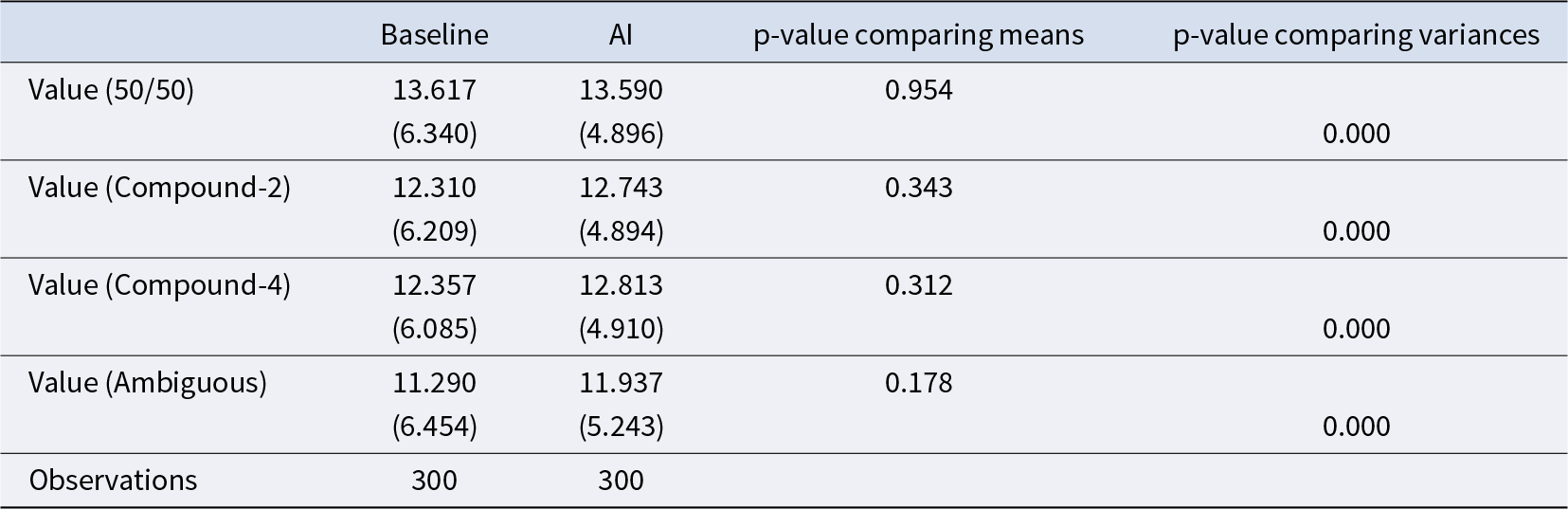
Table 2 summarizes the distribution of valuations by treatment. A clear pattern emerges: mean valuations are unchanged by LLM-based recommendation, while dispersion falls significantly. Mean differences between the Baseline and AI treatments are small and statistically insignificant for every lottery type (t-tests: all 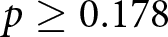 $p \ge 0.178$). In contrast, the equality-of-variance tests reject strongly for every lottery type (pairwise Levene’s tests: all
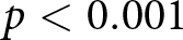 $p \lt 0.001$). Quantitatively, the standard deviation of valuations is about 19–23% lower in the AI-treatment across lotteries (50/50: 6.34 vs. 4.90; Compound-2: 6.21 vs. 4.89; Compound-4: 6.09 vs. 4.91; Ambiguous: 6.45 vs. 5.24), corresponding to a roughly 34–40% reduction in variance with LLM-based recommendation. Thus, LLM-based recommendations primarily compress the cross-participant distribution of valuations rather than shifting average certainty equivalents.
Treatment effect

Table 2 Long description
Mean values and standard deviations are listed for Baseline and AI for four rows labeled Value, followed by a p-value column comparing means and a p-value column comparing variances. For Value 50 slash 50, the Baseline mean is 13.617 with standard deviation 6.340, and the AI mean is 13.590 with standard deviation 4.896; the p-value comparing means is 0.954 and the p-value comparing variances is 0.000. For Value Compound-2, Baseline is 12.310 with 6.209 and AI is 12.743 with 4.894; the p-value comparing means is 0.343 and the p-value comparing variances is 0.000. For Value Compound-4, Baseline is 12.357 with 6.085 and AI is 12.813 with 4.910; the p-value comparing means is 0.312 and the p-value comparing variances is 0.000. For Value Ambiguous, Baseline is 11.290 with 6.454 and AI is 11.937 with 5.243; the p-value comparing means is 0.178 and the p-value comparing variances is 0.000. Observations are 300 for Baseline and 300 for AI.
Notes: In columns 1-2, we report the mean and standard deviation of values participants assign to each lottery in the Baseline and AI treatment, respectively. In columns 3-4, we report the p-values from the t-test for the mean comparisons, and the pairwise Levene’s robust test for the equality of variances, respectively.
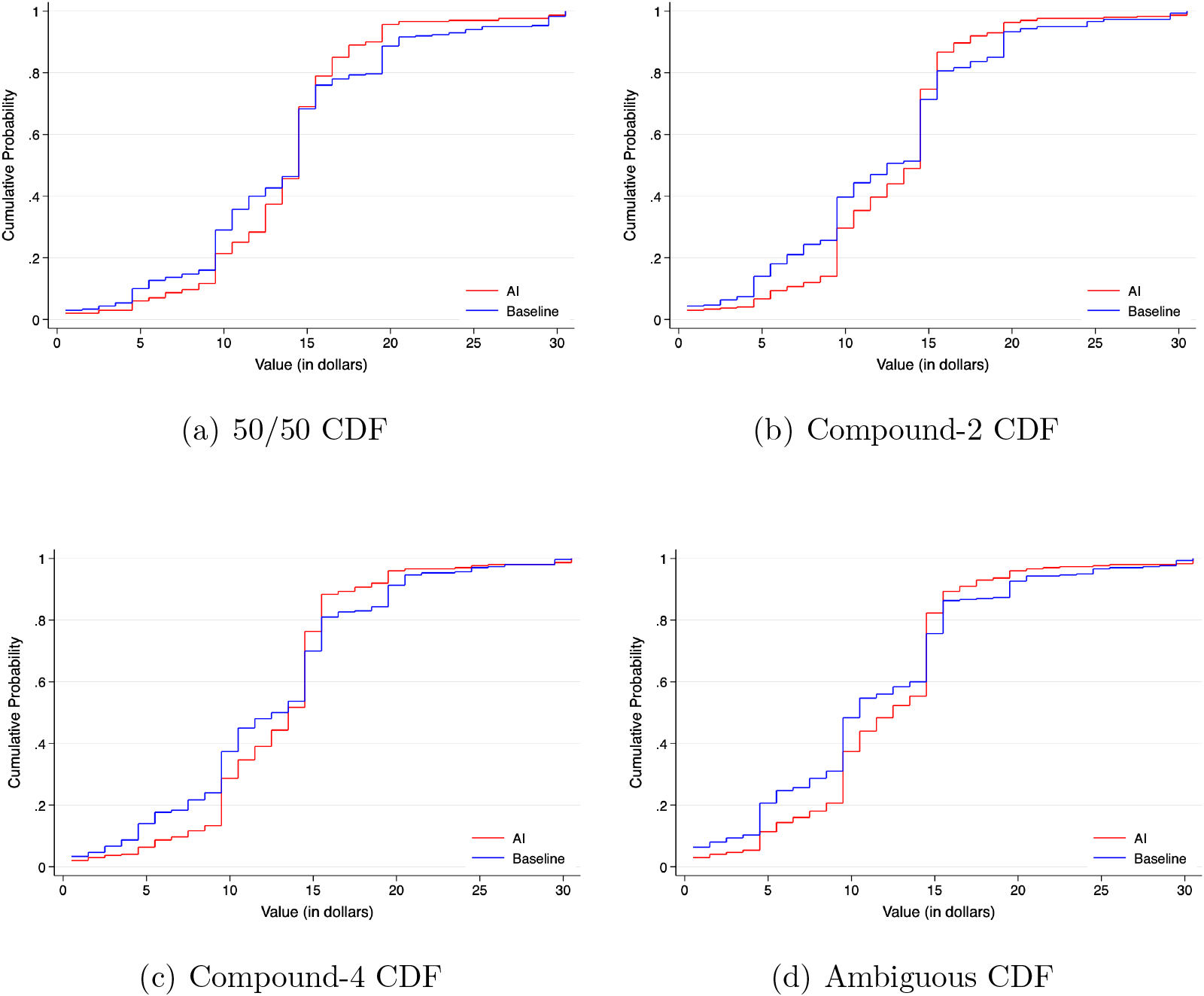
Figure 5 visualizes this compression by plotting the cumulative distribution functions (CDF) of elicited values in the two treatments for each lottery type. Across all lotteries, the CDFs in the AI treatment are steeper in the center and have thinner tails, consistent with fewer extreme valuations and a tighter distribution of risk, complexity, and ambiguity attitudes. In other words, all of the Baseline treatment distributions behave like a mean-preserving spread of the corresponding AI treatment distribution. Applying the Barrett and Donald (Reference Barrett and Donald2003) second-order stochastic dominance test to all CDF comparisons further validates second-order stochastic dominance between the AI and Baseline treatments distributions (using the code from Lee & Whang, Reference Lee and Whang2023).
Baseline vs. AI treatments, CDFs of values

Fig. 5 Long description
A showing a multi-line graph titled 50/50 CDF. The horizontal axis is labeled Value in dollars, ranging from 0 to 25. The vertical axis is labeled Cumulative Probability, ranging from 0 to 1. The AI line generally shows higher cumulative probabilities than the Baseline line, especially around 10 dollars. B showing a multi-line graph titled Compound-2 CDF. The AI line is higher than the Baseline line at lower values, diverging most around 15 dollars. C showing a multi-line graph titled Compound-4 CDF. The AI line shows a steeper increase than the Baseline line, with notable separation around 20 dollars. D showing a multi-line graph titled Ambiguous CDF. The AI line is consistently higher than the Baseline line, with the largest difference around 5 dollars. Each graph uses distinct line styles to differentiate AI and Baseline, as indicated in the legend.
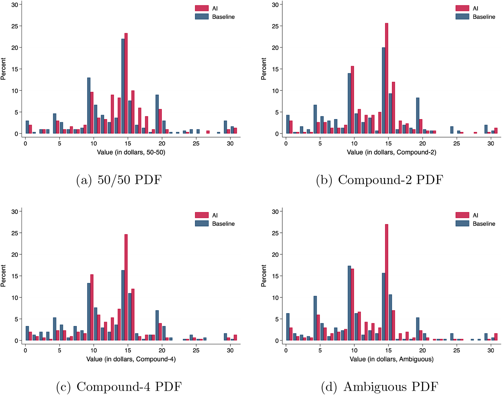
Figure 6 plots corresponding probability distribution functions (PDFs) of the values of each lottery type. Across all lotteries, the PDFs are narrower in the AI treatment complementing the results based on the CDFs.
Baseline vs. AI treatments, PDFs of values

Fig. 6 Long description
Four bar charts comparing AI and Baseline percent distributions for different PDFs. Each chart has the horizontal axis labeled as Value in dollars and the vertical axis labeled as Percent. (a) 50/50 PDF: AI and Baseline distributions with peaks around 15 dollars. AI has a higher peak at this value compared to Baseline. Secondary peaks are visible around 5 and 25 dollars. (b) Compound-2 PDF: A significant peak for AI at 15 dollars, higher than Baseline. Baseline shows a more even distribution with smaller peaks around 10 and 20 dollars. (c) Compound-4 PDF: Both AI and Baseline have peaks at 15 dollars, but AI′s peak is more pronounced. Additional peaks are seen around 10 and 20 dollars, with AI consistently higher. (d) Ambiguous PDF: AI and Baseline both peak at 15 dollars, with AI showing a slightly higher percentage. Smaller peaks occur around 10 and 20 dollars. Across all charts, AI generally shows higher peaks at key values compared to Baseline, indicating a narrower distribution. The legend differentiates AI and Baseline, but specific visual styles are not described. The charts collectively illustrate how AI treatments result in more concentrated value distributions compared to Baseline.
To quantify the reduction in extreme valuations while controlling for participants’ observable characteristics, Table 3 reports four separate regressions, one for each lottery type. In each regression, the dependent variable is the absolute deviation of the participant’s valuation from the midpoint of the elicitation grid,  $|Value-15.5|$. We estimate the regressions separately by lottery type to show that the reduction in distance from the neutral benchmark is not driven by a particular lottery. This presentation mirrors the lottery-specific distributional comparisons in Figures 5 and 6, and the variance comparisons in Table 2. Consistent with the distributional evidence above, LLM-based recommendations significantly reduce absolute deviations from the neutral benchmark for all four lotteries. This indicates that the tightening of valuations reflects a reduction in extreme valuations rather than a uniform shift in stated values.
Regression: Absolute distance to risk-neutrality value

Table 3 Long description
Dependent variable is the absolute distance between each participants valuation and the risk neutral benchmark. Four separate columns report results for lottery types, 50/50, Compound-2, Compound-4, and Ambiguous. In the AI row, coefficients are minus 1.39 with three stars for 50/50, minus 1.36 with three stars for Compound-2, minus 1.23 with three stars for Compound-4, and minus 1.30 with three stars for Ambiguous. Robust standard errors in parentheses are 0.33, 0.34, 0.33, and 0.36, in the same column order. The Demographics row is Yes in all four columns. Observations are 599 in each column.
Notes: Each column reports a separate OLS regression for the corresponding lottery type. The dependent variable is the absolute distance between participant  $i$’s valuation for that lottery and the risk-neutral benchmark,
 $|\text{Value}-15.5|$. One participant with missing demographic information is excluded from the regressions. Robust standard errors are in parentheses. *
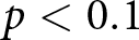 $p \lt 0.1$, **
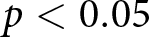
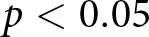 $p \lt 0.05$, ***
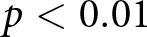
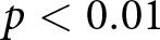 $p \lt 0.01$.
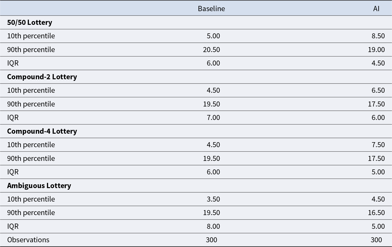
Furthermore, Table 4 reports the 10th and 90th percentile values as well as the interquartile range (IQR), defined as the difference between the 75th and 25th percentiles. In all four lotteries, the 10th percentile is higher in the AI treatment and the 90th percentile is lower in the AI treatment. The IQR is also lower in the AI treatment for all lotteries. These patterns provide additional evidence that LLM-based recommendations compress the valuation distributions.Footnote 7
Extreme percentiles and IQR

Table 4 Long description
Baseline and AI columns report the 10th percentile, 90th percentile, and IQR for four lottery types, plus observations. For 50/50 Lottery, Baseline has 10th percentile 5.00, 90th percentile 20.50, and IQR 6.00; AI has 10th percentile 8.50, 90th percentile 19.00, and IQR 4.50. For Compound-2 Lottery, Baseline is 4.50, 19.50, and 7.00; AI is 6.50, 17.50, and 6.00. For Compound-4 Lottery, Baseline is 4.50, 19.50, and 6.00; AI is 7.50, 17.50, and 5.00. For Ambiguous Lottery, Baseline is 3.50, 19.50, and 8.00; AI is 4.50, 16.50, and 5.00. Observations are 300 for Baseline and 300 for AI.
Hence, the following result is robustly observed in our data:
Result 1: The LLM-based recommendations reduce the heterogeneity in participants’ lottery valuations toward the Baseline mean without shifting the mean.
3.2. Attitudes toward risk, complexity, and ambiguity
Section 3.1 showed that LLM-based recommendations leave average valuations unchanged while compressing the distribution of valuations across participants. A natural next question is whether LLM-based recommendations mitigate risk aversion, complexity aversion, or ambiguity aversion.
Following the literature, we classify participants using the elicited certainty equivalents. A participant is classified as risk-averse if her value for the 50/50 lottery is below the risk-neutral benchmark of 15.5, risk neutral if it equals 15.5, and risk loving if it exceeds 15.5. For complexity attitudes, we compare the value of each compound lottery to the participant’s value for the 50/50 lottery. A participant is classified as complexity averse if the compound-lottery value is lower than the 50/50 value, neutral if the two values are equal, and loving if the compound-lottery value is higher. For ambiguity attitudes, we analogously compare the value of the ambiguous lottery to the value of the 50/50 lottery: lower values indicate ambiguity aversion, equal values indicate ambiguity neutrality, and higher values indicate ambiguity seeking. In the Baseline treatment, the mean valuations for the 50/50, Compound-2, and Compound-4 lotteries reported in Table 2 are all below 15.5, the risk-neutral benchmark (Wilcoxon signed-rank test: all 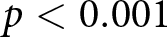 $p \lt 0.001$). The participants are ambiguity averse on average in the Baseline, too: the ambiguous lottery is valued less than the 50/50 lottery (Wilcoxon signed-rank test
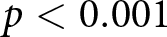 $p \lt 0.001$). Consistent with the evidence in de Clippel et al. (Reference de Clippel, Moscariello, Ortoleva and Rozen2024), we also observe aversion to complexity in the Baseline: The average valuations for both Compound-2 and Compound-4 are significantly lower than the average valuation of the 50/50 lottery (Wilcoxon signed-rank tests
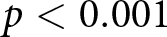 $p \lt 0.001$). We observe the same qualitative pattern in the AI treatment: average valuations remain below \$15.5 for the 50/50 lottery and are further discounted for compound risk and ambiguity relative to the 50/50 benchmark, indicating risk aversion, complexity aversion, and ambiguity aversion (Wilcoxon signed-rank tests all
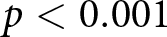 $p \lt 0.001$).
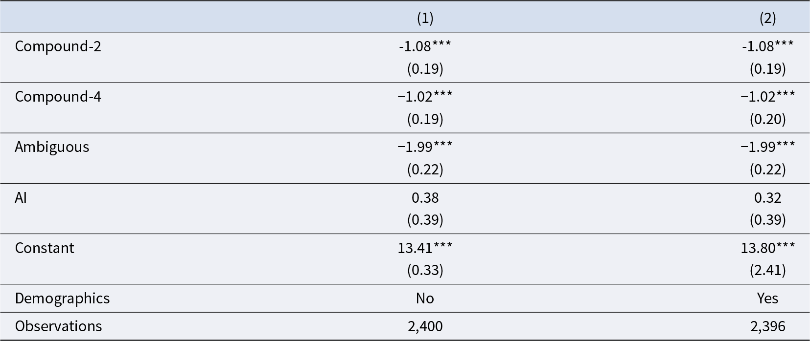
Complexity and ambiguity aversion are robust to controlling for demographics. Table 5 estimates regressions where the 50/50 lottery is the control category. In the Baseline treatment, valuations for Compound-2 and Compound-4 are significantly lower than for the 50/50 lottery, consistent with complexity aversion: holding expected value fixed, participants value compound risk less than simple risk. Valuations for the Ambiguous lottery are also lower than for the 50/50 lottery, consistent with ambiguity aversion on average. The treatment variable (AI treatment dummy variable) is statistically insignificant, consistent with the results of Section 3.1.Footnote 8
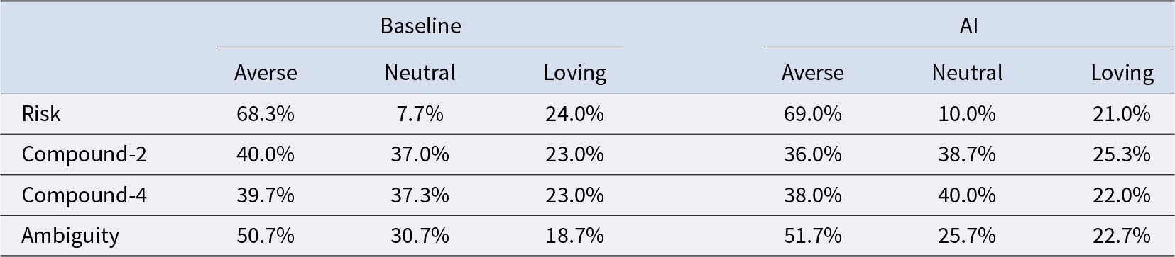
Table 6 classifies participants by their risk, complexity, and ambiguity attitudes in both the Baseline and AI treatments, and the shares in each category are very similar across treatments. For example, 68.3% of participants are classified as risk-averse in the Baseline, compared with 69.0% in the AI treatment. These results indicate that AI assistance does not significantly change attitude classifications toward risk, complexity, or ambiguity (Fisher’s exact tests 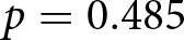 $p=0.485$ in Risk,
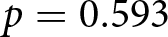 $p=0.593$ in Compound-2,
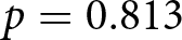 $p=0.813$ in Compound-4,
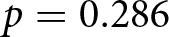 $p=0.286$ in Ambiguity).
Regression: Lottery value

Table 5 Long description
Two regression models labeled, 1 and 2, report coefficients with standard errors in parentheses for Compound 2, Compound 4, Ambiguous, AI, and the Constant. In model 1, Compound 2 is minus 1.08 with three stars and standard error 0.19; Compound 4 is minus 1.02 with three stars and standard error 0.19; Ambiguous is minus 1.99 with three stars and standard error 0.22; AI is 0.38 with standard error 0.39; Constant is 13.41 with three stars and standard error 0.33. In model 2, Compound 2 is minus 1.08 with three stars and standard error 0.19; Compound 4 is minus 1.02 with three stars and standard error 0.20; Ambiguous is minus 1.99 with three stars and standard error 0.22; AI is 0.32 with standard error 0.39; Constant is 13.80 with three stars and standard error 2.41. The Demographics row shows No for model 1 and Yes for model 2. Observations are 2,400 in model 1 and 2,396 in model 2.
Notes: The 50/50 lottery value is the comparison group. One participant with missing demographic information is excluded from the regression. Standard errors are clustered at the subject level. *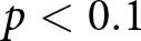 $p \lt 0.1$, **
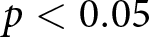 $p \lt 0.05$,
***
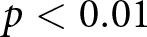 $p \lt 0.01$.
Preference classification, baseline vs. AI

Table 6 Long description
Percentages are reported for three classifications, averse, neutral, and loving, under two conditions labeled Baseline and AI, for four rows: Risk, Compound-2, Compound-4, and Ambiguity. For Risk, Baseline is 68.3% averse, 7.7% neutral, and 24.0% loving; AI is 69.0% averse, 10.0% neutral, and 21.0% loving. For Compound-2, Baseline is 40.0% averse, 37.0% neutral, and 23.0% loving; AI is 36.0% averse, 38.7% neutral, and 25.3% loving. For Compound-4, Baseline is 39.7% averse, 37.3% neutral, and 23.0% loving; AI is 38.0% averse, 40.0% neutral, and 22.0% loving. For Ambiguity, Baseline is 50.7% averse, 30.7% neutral, and 18.7% loving; AI is 51.7% averse, 25.7% neutral, and 22.7% loving.
Notes: Classifications are based on elicited certainty equivalents. Risk attitudes are classified by comparing the value of the 50/50 lottery to the risk-neutral benchmark of 15.5. Complexity attitudes are classified by comparing the value of each compound lottery to the participant’s value for the 50/50 lottery. Ambiguity attitudes are classified by comparing the value of the ambiguous lottery to the participant’s value for the 50/50 lottery. The neutral category is defined by exact equality on the elicited valuation grid.
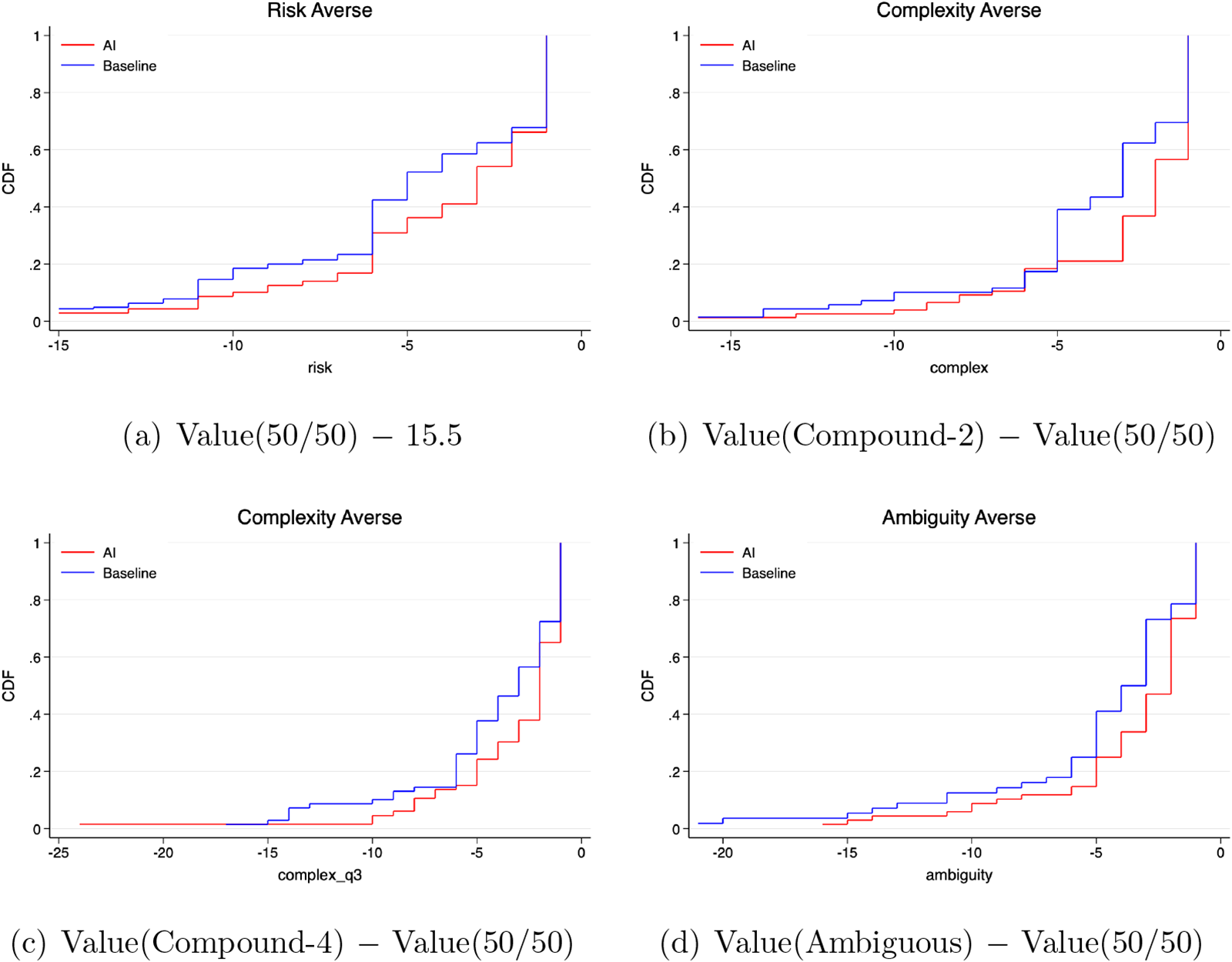
While classifications are stable, the magnitudes of these attitudes shift under LLM-based recommendations. Figures 7a–d plot CDFs of risk, complexity, and ambiguity aversion measures of the participants who are classified as averse, separately. For instance, Figure 7a shows that, among participants classified as risk-averse, the distribution of deviations below the risk neutral benchmark in the AI treatment first-order stochastically dominates the corresponding distribution in the Baseline treatment. In other words, risk-averse participants submit systematically higher valuations under LLM-based recommendations (Mann-Whitney test 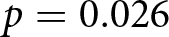 $p=0.026$). The same qualitative pattern appears for complexity averse participants (Figures 7b and 7c; Mann-Whitney tests
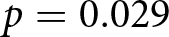 $p=0.029$ and
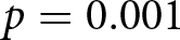 $p=0.001$, respectively), ambiguity averse participants (Figure 7d; Mann-Whitney test
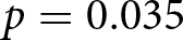 $p=0.035$). Overall, LLM-based recommendations compress the distribution of attitude magnitudes: they make risk-, complexity-, and ambiguity-averse participants less extreme, without changing their classification.
CDFs of the magnitudes of risk, complexity, and ambiguity aversion

Fig. 7 Long description
Four line graphs labeled a, b, c and d, each showing cumulative distribution functions (CDFs) for different aversion measures under AI and Baseline conditions. Graph a, titled ′Risk Averse′, plots risk on the horizontal axis from negative 15 to positive 5, with CDF on the vertical axis. The AI line is generally higher than the Baseline, indicating a shift in distribution. Graph b, titled ′Complexity Averse′, plots complex on the horizontal axis from negative 15 to positive 5. The AI line again tends to be higher, especially around complex equals 0. Graph c, titled ′Complexity Averse′, also plots complex from negative 15 to positive 5, showing a similar pattern with AI dominating Baseline. Graph d, titled ′Ambiguity Averse′, plots ambiguity from negative 15 to positive 5, with the AI line higher, particularly around ambiguity equals 0.5. Each graph includes a legend distinguishing AI and Baseline by line style. The overall purpose is to compare how AI and Baseline conditions shift distributions across different aversion measures, highlighting where AI recommendations lead to higher valuations.
Result 2: The LLM-based recommendations reduce the intensity of risk, complexity, and ambiguity aversion while leaving the distributions of classification as averse/neutral/loving unchanged.
3.3. Discussion: potential mechanisms
Our results show that LLM-based recommendations compress the distribution of elicited valuations without significantly changing the shares of participants classified as risk-, complexity-, or ambiguity-averse. This pattern raises a natural question: what mechanisms would explain the reduction in dispersion?
A first possibility is numerical anchoring or surveyor demand effect. The LLM-based recommendations explicitly highlighted the risk-neutral benchmark. For the risky and compound lotteries, the recommendation explained that the probability of winning is 50% and that the expected value of the lottery is \$15. It also described switching around this value as consistent with risk-neutral behavior. For the ambiguous lottery, the advice similarly discussed a \$15 benchmark under a subjective belief that the expected fraction of purple cards is 50%. These statements could have made the middle of the MPL more salient and pulled extreme valuations toward the center if the subjects interpret this as what they are expected to do.
These anchoring or surveyor demand effect interpretations are consistent with the increase in mass around the neutral switching point in Figure 6. At the same time, the data do not suggest a purely mechanical response in which participants simply copied the benchmark across all questions. Only 13 participants in the AI treatment switched to the sure payment at 15 in all four questions while there were 15 of those participants in the Baseline treatment. Furthermore, participants in the AI treatment often chose different switching points across the four lotteries, indicating that they continued to distinguish among the decision problems rather than applying the same benchmark mechanically. Thus, while benchmark salience may be part of the treatment effect, the evidence suggests partial adjustment toward the benchmark rather than uniform adoption of the LLM-based recommendation. This is also consistent with the Judge-Advisor System literature (see Kämmer et al., Reference Kämmer, Choshen-Hillel, Müller-Trede, Black and Weibler2023 for a survey), which argues that the weight on the advice depends on the complexity of the environment and the engagement of the decision makers with the advice (Rebholz and Hütter, Reference Rebholz and Hütter2022; Rebholz et al., Reference Rebholz, Koop and Hütter2024).
A related possibility is that the recommendations created additional focal points. In several cases, the LLM described switching below \$15, for example in the \$10–\$14 range, as consistent with risk-averse behavior. This may help explain the smaller peak around 10 in the valuation distributions. However, similar round-number peaks also appear in the Baseline treatment and in the data of de Clippel et al. (Reference de Clippel, Moscariello, Ortoleva and Rozen2024), suggesting that part of this pattern may reflect the discrete MPL grid and participants’ general tendency to report round numbers. Again, the response is not fully mechanical: Out of 300 participants, only 11 participants in the AI treatment switched at 10 in all four questions, and this number was 7 in the Baseline treatment.
A second possible mechanism is cognitive offloading. The compound lotteries require participants to reduce a multi-stage lottery to its objective winning probability. The LLM-based recommendations perform this calculation explicitly and explain how the resulting expected-value benchmark should be interpreted. If participants find this reduction cognitively costly, the recommendations may reduce uncertainty about the correct probability calculation and, in turn, attenuate the effect of complexity on valuations. This interpretation is related to Enke and Graeber (Reference Enke and Graeber2023), who argue that biases are less pronounced when cognitive load is lower.
The belief and confidence measures are consistent with this interpretation. Recall that, after each compound lottery, participants reported their belief about the probability of drawing a purple card and how certain they were about that belief on a 0–100% scale. Following de Clippel et al. (Reference de Clippel, Moscariello, Ortoleva and Rozen2024), we define cognitive uncertainty as 100 minus the participant’s certainty score. Table 7 shows that, in the Baseline treatment, participants were less likely to report the correct belief for the more complex Compound-4 lottery than for the Compound-2 lottery (0.70 vs. 0.77, Wilcoxon signed-rank test 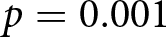 $p=0.001$). They also reported higher cognitive uncertainty for Compound-4 than for Compound-2 (42.10 vs. 37.13, Wilcoxon signed-rank test
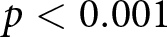 $p \lt 0.001$). Thus, without LLM-based recommendations, participants found the more complex compound lottery harder to evaluate and were less confident in their beliefs.
Belief and cognitive uncertainty

Table 7 Long description
Measures two outcomes, Correct Belief and Cognitive Uncertainty, each reported for Compound-2 and Compound-4, with rows for Baseline and AI. For Baseline, Correct Belief is 0.77 for Compound-2 and 0.70 for Compound-4. For AI, Correct Belief is 0.73 for Compound-2 and 0.75 for Compound-4. For Baseline, Cognitive Uncertainty is 37.13 for Compound-2 and 42.10 for Compound-4. For AI, Cognitive Uncertainty is 36.43 for Compound-2 and 35.80 for Compound-4.
Notes:  $N=300$ in each treatment. Cognitive uncertainty is defined as 100 minus the participant’s reported certainty about their belief.
In the AI treatment, these complexity-related gaps disappear. Correct-belief rates are statistically similar for Compound-2 and Compound-4 (0.73 vs. 0.75, Wilcoxon signed-rank test 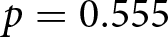 $p=0.555$), and cognitive uncertainty is no longer higher for Compound-4 (36.43 vs. 35.80, Wilcoxon signed-rank test
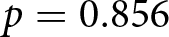 $p=0.856$). This pattern suggests that LLM-based recommendations reduced the additional cognitive burden created by the more complex compound lottery.
For robustness, we compute, for each participant, the difference in cognitive uncertainty between Compound-4 and Compound-2 and regress this difference on the AI treatment indicator. Table 8 shows that the AI coefficient is negative and statistically significant, with or without demographic controls. This indicates that LLM-based recommendations reduce the additional cognitive uncertainty associated with the more complex compound lottery.
Regression: Difference in cognitive uncertainty between Compound-4 and Compound-2

Table 8 Long description
Outcome is cognitive uncertainty for Compound 4 minus cognitive uncertainty for Compound 2, reported for two models labeled column 1 and column 2. Row, AI reports a coefficient of minus 5.60 with three asterisks in column 1 and minus 5.68 with three asterisks in column 2. The standard errors shown beneath AI are 1.51 for column 1 and 1.52 for column 2. Row, Demographics indicates No in column 1 and Yes in column 2. Row, Observations lists 600 in column 1 and 599 in column 2.
Notes: The dependent variable is cognitive uncertainty for Compound-4 minus cognitive uncertainty for Compound-2. One participant with missing demographic information is excluded from column (2). Robust standard errors are in parentheses. *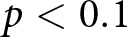 $p \lt 0.1$, **
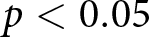 $p \lt 0.05$, ***
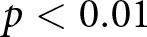 $p \lt 0.01$.
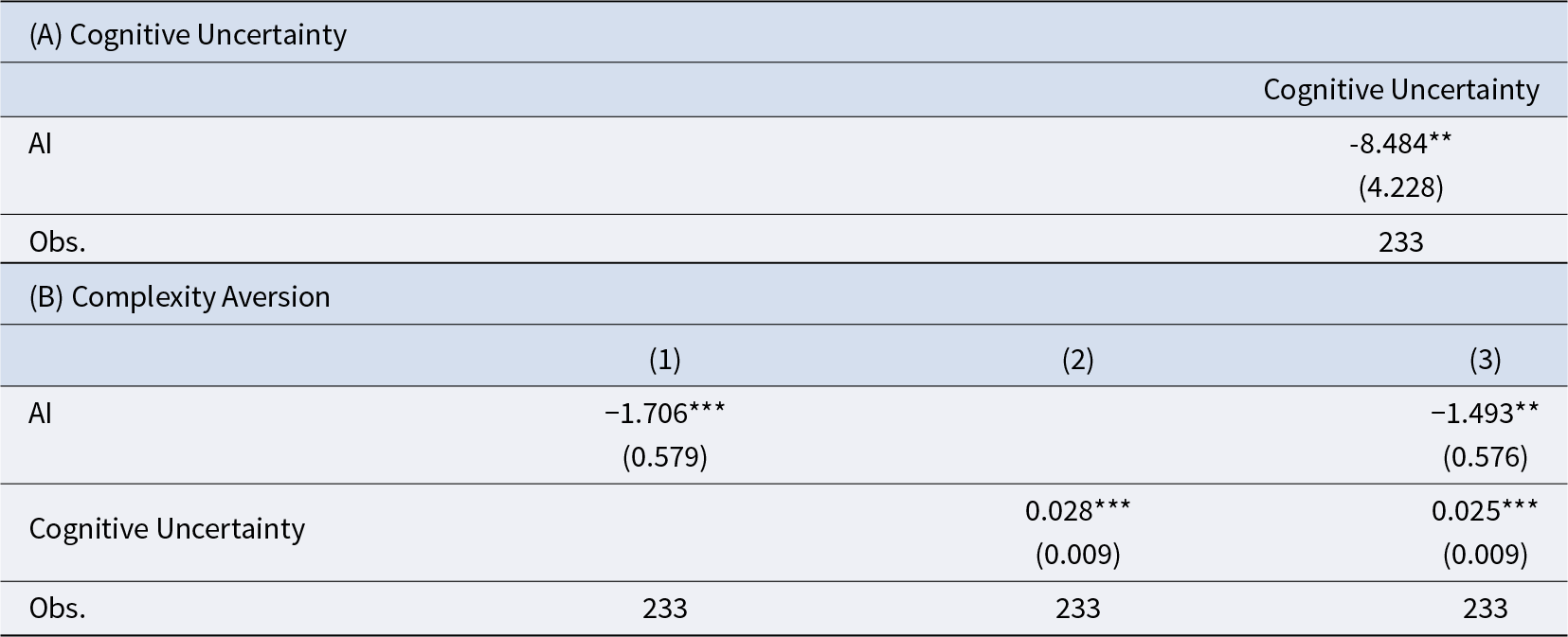
Table 9(A) shows that the relationship between cognitive uncertainty and complexity aversion is also consistent with the cognitive-offloading interpretation for the Compound-4 lottery. Among participants classified as complexity averse based on Compound-4 behavior, Table 9(B) shows that both the AI treatment indicator and lower cognitive uncertainty are associated with a smaller magnitude of complexity aversion. This relationship persists when both variables are included in the same regression. Hence, cognitive offloading is one channel through which LLM-based recommendations attenuate the intensity of complexity aversion as it complements (Enke and Graeber, Reference Enke and Graeber2023).
Complexity aversion and cognitive uncertainty

Table 9 Long description
Cognitive uncertainty is reported with one predictor row labeled, AI, and one row for the number of observations. For AI, the coefficient is minus 8.484 with two asterisks. The standard error shown beneath that coefficient is 4.228 in parentheses. The observations row lists 233.
Notes: Regressions are for the complexity averse subjects, those with the Compound-4 value lower than 50/50 Lottery value. Dependent variable is cognitive uncertainty in panel (A) and the magnitude of complexity aversion in panel (B). Robust standard errors are in parentheses. *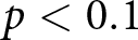 $p \lt 0.1$, **
 $p \lt 0.05$, ***
 $p \lt 0.01$.
4. Conclusion
This paper experimentally studies how LLM-based recommendations affect evaluations of uncertainty. Our main result is that providing participants with lottery-specific recommendations from a large language model changes valuations in a second-order stochastic dominance sense: across lotteries, LLM-based recommendation leaves average certainty equivalents unchanged, but it systematically reduces dispersion.
Our findings have two direct implications for economic research and practice. First, they speak directly to the measurement of preferences. Risk and ambiguity preferences are routinely elicited to discipline models, calibrate welfare, and predict behavior in markets and policy settings. Our evidence indicates that when an economically relevant choice environment includes readily available LLM-based recommendations, as it increasingly does, standard elicitation procedures may recover preferences as expressed with AI mediation. This may directly impact risk profiling procedures, which are frequently used by investment platforms.
Second, these results contribute to the economics of complexity in decision making under uncertainty. We compare lotteries that imply the same objective risk but differ in computational burden, and we also consider lotteries that introduce ambiguity. Across these settings, we find that the first result above continues to hold robustly. Since real-world decision environments are often more complex and complexity itself is one of the key drivers of AI adoption, our finding that LLM-based recommendations reduce heterogeneity in the magnitude of risk and ambiguity attitudes has direct implications for applied contexts, including insurance choice and retirement planning.
Finally, as we implement a tightly controlled LLM-based recommendation treatment in which all participants view the same pre-generated GPT screenshots, produced from a single prompt (“What do you recommend for someone making these choices?”), it strengthens internal validity by eliminating endogenous prompting and heterogeneity in prompt quality. It also enhances replicability by fixing the recommendation content. Importantly, exposure to identical recommendations does not mechanically anchor participants to the same response. Instead, LLM-based recommendation preserves the qualitative structure of heterogeneity in risk, complexity, and ambiguity attitudes, as participants remain meaningfully dispersed and ordered in their preferences while attenuating the magnitudes of these attitudes by compressing the tails of the valuation distribution.
A natural next step is to study less standardized forms of AI advice. Our design fixes the content of the LLM-based recommendation across participants within each lottery. This strengthens internal validity and replicability by eliminating endogenous prompting, variation in prompt quality, and variation in follow-up interactions, but it limits external validity relative to real-world AI use, where recommendations may vary across calls and users may interact with the model in different ways.
Future work could implement intermediate designs between our fixed-advice treatment and fully endogenous AI use. For example, researchers could generate participant-specific recommendations in real time while holding the prompt fixed, or pre-generate multiple recommendations for each lottery using the same prompt and randomize which version participants see. These approaches would preserve control over prompting while allowing recommendation content to vary across observations, thereby testing whether the compression of valuations attenuates, disappears, or persists when advice varies across LLM calls. In less structured decision problems, endogenous AI use may also have different effects because advice uptake can depend on whether advice is expected and how it is explained, as emphasized by Rebholz et al. (Reference Rebholz, Koop and Hütter2024). More broadly, as AI systems become embedded in consumer finance, insurance markets, and medical decision support, understanding how recommendations reshape decisions under uncertainty and what aspects of preferences they change will be essential for both modeling and policy design.
Supplementary material
The supplementary material for this article can be found at https://doi.org/10.1017/eec.2026.10062.
Replication material
The replication materials for this study are available at https://osf.io/we2rg.
Acknowledgements
The authors acknowledge using ChatGPT 5.2. to improve grammar and word choice in the manuscript. AI was not used elsewhere in the writing of the manuscript. The authors take full responsibility for the content. All final wording reflects the authors’ judgment. We would like to thank Bakican Ayna, Quang Pham, and Joseph Tao-yi Wang for helpful comments and discussions. All errors are our own.
Funding statement
We are thankful to the University of Maryland College of Behavioral and Social Sciences for the generous funding used for participant payments.





 Open access

