1 Introduction
Polymer solutions can exhibit a chaotic behaviour, even at low Reynolds numbers, as a result of purely elastic instabilities (Groisman & Steinberg Reference Groisman and Steinberg2000, Reference Groisman and Steinberg2004). This regime of polymer solutions, known as elastic turbulence, finds a natural application in microfluidics, where the typical Reynolds numbers are very low and the addition of polymers to the fluid can be employed to accelerate phenomena such as mixing (Groisman & Steinberg Reference Groisman and Steinberg2001), emulsification (Poole et al. Reference Poole, Budhiraja, Cain and Scott2012) and heat transfer (Traore, Castelain & Burghelea Reference Traore, Castelain and Burghelea2015; Abed et al. Reference Abed, Whalley, Dennis and Poole2016) or to examine the dynamics of microscopic objects in fluctuating flows (Liu & Steinberg Reference Liu and Steinberg2014).
The numerical simulation of elastic turbulence is challenging for at least three reasons. The first two are common to the high-Reynolds-number regime of polymer solutions. Indeed, the available constitutive models of viscoelastic fluids are based on rather crude approximations and disregard several, potentially relevant aspects of polymer dynamics (Bird et al. Reference Bird, Hassager, Armstrong and Curtiss1987). In addition, a high spatial resolution and advanced numerical schemes are needed to resolve the sharp gradients that form in the polymer-stress field (Jin & Collins Reference Jin and Collins2007; Plan et al. Reference Plan, Gupta, Vincenzi and Gibbon2017). The third reason is specific to elastic turbulence and is the requirement that the time step used for the integration of the Navier–Stokes equations be small; this requirement is a consequence of the high viscosity of the fluid (Press et al. Reference Press, Teukolsky, Vetterling and Flannery2007).
Most numerical studies of elastic turbulence have therefore considered simplified flow configurations (e.g. in two dimensions and/or with periodic boundary conditions) and have been restricted to limited ranges of parameters. Notwithstanding, even simple models of viscoelastic fluids in idealized settings have proved successful in capturing the main properties of elastic turbulence. Several experimental observations are reproduced, at least qualitatively, by the Oldroyd-B model, in which only the slowest oscillation mode of the polymer is retained and polymer elasticity is assumed to be linear (Berti et al. Reference Berti, Bistagnino, Boffetta, Celani and Musacchio2008; Thomases & Shelley Reference Thomases and Shelley2009; Berti & Boffetta Reference Berti and Boffetta2010; Thomases, Shelley & Thiffeault Reference Thomases, Shelley and Thiffeault2011; Grilli, Vázquez-Quesada & Ellero Reference Grilli, Vázquez-Quesada and Ellero2013; Plan et al. Reference Plan, Gupta, Vincenzi and Gibbon2017; van Buel, Schaaf & Stark Reference van Buel, Schaaf and Stark2018; Garg et al. Reference Garg, Calzavarini, Mompean and Berti2018). Other studies have used the FENE-P model, which improves on the Oldroyd-B one by taking into account the finite extensibility of polymers (Liu & Khomami Reference Liu and Khomami2013; Gupta & Pandit Reference Gupta and Pandit2017), or have taken a Lagrangian approach and have solved the dynamics of a large number of dumbbell-like polymers (Watanabe & Gotoh Reference Watanabe and Gotoh2013, Reference Watanabe and Gotoh2014). In fact, even a low-dimensional ‘shell model’ of viscoelastic fluid reproduces elastic turbulence qualitatively (Ray & Vincenzi Reference Ray and Vincenzi2016).
Constitutive models such as the Oldroyd-B and the FENE-P ones consist of a coupled system of partial differential equations for the velocity of the solution and for the polymer stress tensor. This latter is by nature positive definite, but numerical errors may lead to the loss of this property and hence to instabilities (Joseph Reference Joseph1990). A standard way to prevent such instabilities is to include global artificial diffusivity in the model, i.e. to add a Laplacian term to the evolution equation for the polymer stress with a space-independent coefficient (Sureshkumar & Beris Reference Sureshkumar and Beris1995). Numerical simulations of turbulent polymer solutions that use artificial diffusivity are in qualitative agreement with experiments (e.g. Graham Reference Graham2014, and references therein). Polymer-stress diffusion in fact has a physical origin, for it results from the diffusion of the centre of mass of polymers due to thermal noise (El-Kareh & Leal Reference El-Kareh and Leal1989). However, the values of diffusivity needed to achieve numerical stability are three to six orders of magnitude greater than those appropriate for real polymers (e.g. Vaithianathan et al. Reference Vaithianathan, Robert, Brasseur and Collins2006). For this reason, numerical schemes have been proposed that avoid using artificial diffusivity. These include, inter alia, schemes that only employ polymer diffusivity at those locations in the fluid where the polymer stress loses its positive-definite character (Min, Yoo & Choi Reference Min, Yoo and Choi2001), methods adapted from hyperbolic solvers (Vaithianathan et al. Reference Vaithianathan, Robert, Brasseur and Collins2006) or schemes based on representations of the polymer stress tensor that guarantee the preservation of its positive definiteness (Fattal & Kupferman Reference Fattal and Kupferman2003; Vaithianathan & Collins Reference Vaithianathan and Collins2003; Balci et al. Reference Balci, Thomases, Renardy and Doering2011; Hameduddin et al. Reference Hameduddin, Meneveau, Zaki and Gayme2018). Such numerical schemes have been compared with simulations using artificial diffusivity at high or moderate Reynolds numbers, and quantitative discrepancies have emerged: for instance, the level of drag reduction is diminished by artificial diffusivity, the velocity and polymer-stress fields are significantly smeared and excessive polymer-stress diffusion leads to relaminarization (Min et al. Reference Min, Yoo and Choi2001; Vaithianathan et al. Reference Vaithianathan, Robert, Brasseur and Collins2006; Sid, Terrapon & Dubief Reference Sid, Terrapon and Dubief2018). Thus a consensus seems to have formed that at high or moderate Reynolds numbers alternative methods should be preferred to the use of artificial diffusivity.
At low Reynolds numbers, several studies of elastic turbulence have employed artificial diffusivity (Berti et al. Reference Berti, Bistagnino, Boffetta, Celani and Musacchio2008; Thomases & Shelley Reference Thomases and Shelley2009; Berti & Boffetta Reference Berti and Boffetta2010; Thomases et al. Reference Thomases, Shelley and Thiffeault2011; Liu & Khomami Reference Liu and Khomami2013; Garg et al. Reference Garg, Calzavarini, Mompean and Berti2018). It was shown in Thomases (Reference Thomases2011) that in viscoelastic creeping flows this has the effect of smoothing the polymer-stress field and keeping it bounded. However, to the best of our knowledge, the effect of artificial diffusivity in the elastic turbulence regime has not been examined yet. This is the object of the present study, in which we compare numerical simulations with and without artificial diffusivity. As a case study, we consider the Oldroyd-B model with a cellular forcing on a periodic square (analogous simulations of the FENE-P model are presented in appendix A). The cellular forcing generates distinct regions of straining and vorticity and thus allows us to describe a flow configuration in which the effect of artificial diffusivity is particularly adverse. Our results demonstrate that the properties of the velocity field are strongly affected, to such an extent that also the large-scale flow may be misrepresented. In particular, we show that some phenomena observed in previous simulations are due to artificial stress diffusion and are not present when alternative integration methods are used.
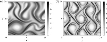
The general effect of artificial diffusivity is to spread high polymer stresses over large regions of the flow, including those where the polymer stress would be weak because vorticity dominates and polymers should not be stretched. We shall see that, in elastic turbulence, this fact leads to a spurious symmetry breaking analogous to that observed in Thomases & Shelley (Reference Thomases and Shelley2009) and Thomases et al. (Reference Thomases, Shelley and Thiffeault2011). Indeed, in low-strain regions polymers are weakly stretched and the external force would naturally impose its spatial structure, but if high polymer stresses artificially diffuse into those regions, they prevail over the force and provoke a strong modification of the large-scale flow. This dynamics is specific to elastic turbulence, because the Reynolds number is low and, in the absence of artificial diffusivity, the original laminar flow is weakly perturbed by the addition of polymers in vorticity-dominated regions. At high Reynolds numbers the effect of artificial diffusivity is less dramatic, since the flow is already chaotic before the addition of polymers and therefore artificial diffusivity does not change the large-scale flow so strongly. Indeed, at high Reynolds numbers, the differences between simulations with and without artificial diffusivity are essentially quantitative (Vaithianathan et al. Reference Vaithianathan, Robert, Brasseur and Collins2006; Sid et al. Reference Sid, Terrapon and Dubief2018). In conclusion, we show that in elastic turbulence artificial diffusivity induces dramatic qualitative modifications of the large-scale flow, which are not observed at high Reynolds numbers. Hence the study of the low-Reynolds-number regime requires a separate study.
2 Viscoelastic model
The Oldroyd-B model (Oldroyd Reference Oldroyd1950) describes the deformation of polymers by means of a space–time-dependent positive-definite tensor: the polymer conformation tensor
 $\unicode[STIX]{x1D63E}(\boldsymbol{x},t)$
. In the limit of vanishing inertia, the coupled evolution of
 $\unicode[STIX]{x1D63E}(\boldsymbol{x},t)$
and the velocity field
 $\boldsymbol{u}(\boldsymbol{x},t)$
that describes the motion of the solution is given by the following equations:
 $$\begin{eqnarray}\displaystyle & \displaystyle \unicode[STIX]{x1D735}p=\unicode[STIX]{x1D708}\unicode[STIX]{x0394}\boldsymbol{u}+{\displaystyle \frac{\unicode[STIX]{x1D707}}{\unicode[STIX]{x1D70F}}}\,\unicode[STIX]{x1D735}\boldsymbol{\cdot }\unicode[STIX]{x1D63E}+\boldsymbol{f},\quad \unicode[STIX]{x1D735}\boldsymbol{\cdot }\boldsymbol{u}=0, & \displaystyle\end{eqnarray}$$
 $$\begin{eqnarray}\displaystyle & \displaystyle \unicode[STIX]{x2202}_{t}\unicode[STIX]{x1D63E}+\boldsymbol{u}\boldsymbol{\cdot }\unicode[STIX]{x1D735}\unicode[STIX]{x1D63E}=(\unicode[STIX]{x1D735}\boldsymbol{u})\boldsymbol{\cdot }\unicode[STIX]{x1D63E}+\unicode[STIX]{x1D63E}\boldsymbol{\cdot }(\unicode[STIX]{x1D735}\boldsymbol{u})^{\top }-{\displaystyle \frac{1}{\unicode[STIX]{x1D70F}}}(\unicode[STIX]{x1D63E}-\unicode[STIX]{x1D644}), & \displaystyle\end{eqnarray}$$
 $p$
is pressure,
 $\unicode[STIX]{x1D708}$
is the kinematic viscosity of the solvent,
 $\unicode[STIX]{x1D70F}$
is the polymer relaxation time, the components of the velocity gradient are defined as
 $(\unicode[STIX]{x1D735}\boldsymbol{u})_{ij}=\unicode[STIX]{x2202}u_{i}/\unicode[STIX]{x2202}x_{j}$
and
 $\unicode[STIX]{x1D644}$
is the identity matrix. The coupling coefficient
 $\unicode[STIX]{x1D707}$
represents the polymer contribution to the total kinematic viscosity of the solution and is proportional to the concentration of polymers. The body force
 $\boldsymbol{f}(\boldsymbol{x})$
that sustains the motion of the solution is such that
 $\unicode[STIX]{x1D735}\boldsymbol{\cdot }\boldsymbol{f}=0$
. In the above equations, the conformation tensor is rescaled with the polymer mean square equilibrium extension in the absence of flow.
In considering the limit of the Oldroyd-B model for vanishing inertia, we follow Fouxon & Lebedev (Reference Fouxon and Lebedev2003), Thomases & Shelley (Reference Thomases and Shelley2009), Thomases et al. (Reference Thomases, Shelley and Thiffeault2011) and Balci et al. (Reference Balci, Thomases, Renardy and Doering2011), who describe the motion of the solution by means of the Stokes equations in lieu of the Navier–Stokes equations. However, as is discussed in § 4, our conclusions on the effect of artificial diffusivity are unchanged if we use the Navier–Stokes equations with a Reynolds number smaller than the critical value for the appearance of inertial instabilities.
Equations (2.1) are studied on the two-dimensional domain
 $V=[0,2\unicode[STIX]{x03C0}]^{2}$
with periodic boundary conditions. We consider the cellular force
 $$\begin{eqnarray}\boldsymbol{f}(\boldsymbol{x})=f_{0}(-\sin Ky,\sin Kx),\end{eqnarray}$$
where
 $f_{0}$
is the amplitude and
 $K$
the spatial frequency. Cellular-like forcings have been widely used in experiments of chaotic mixing in two-dimensional flows (e.g. Cardoso, Marteau & Tabeling Reference Cardoso, Marteau and Tabeling1994; Rothstein, Henry & Gollub Reference Rothstein, Henry and Gollub1999). As is discussed in § 4, the effect of artificial diffusivity for other forcings may not be equally dramatic; however, the cellular forcing allows us to clearly identify the fashion in which artificial diffusivity operates in elastic turbulence and to demonstrate how strong its effect can be in this regime.
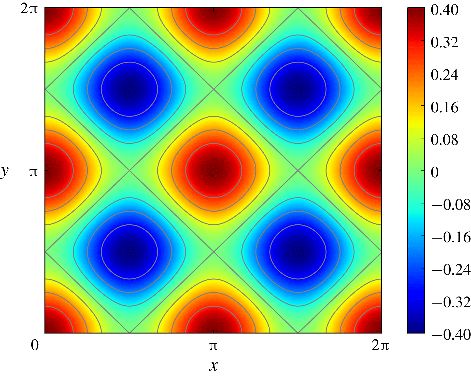
Vorticity field of the laminar solution of (2.1a
) in the absence of polymer feedback,
 $\unicode[STIX]{x1D714}(\boldsymbol{x})=-f_{0}(\cos Kx+\cos Ky)/\unicode[STIX]{x1D708}K$
, for
 $K=2$
,
 $f_{0}=0.02$
and
 $\unicode[STIX]{x1D708}=0.05$
.

In the absence of polymer feedback on the flow (i.e.
 $\unicode[STIX]{x1D707}=0$
), (2.1a
) admits the fixed-point laminar solution:
 $\boldsymbol{u}=-\boldsymbol{f}/\unicode[STIX]{x1D708}K^{2}$
. The corresponding vorticity field
 $\unicode[STIX]{x1D714}(\boldsymbol{x},t)$
, where
 $\unicode[STIX]{x1D714}\hat{\boldsymbol{z}}\equiv \unicode[STIX]{x1D735}\times \boldsymbol{u}$
, is shown in figure 1 and consists of a sequence of vortices of alternate sign separated by lines of pure strain. At time
 $t=0$
,
 $\boldsymbol{u}$
is the fixed-point velocity field and
 $\unicode[STIX]{x1D63E}$
is a perturbation of the identity matrix (we use the same perturbation as in Thomases & Shelley Reference Thomases and Shelley2009; see their equation (3)). By using the length scale
 $1/K$
and the amplitude
 $f_{0}/\unicode[STIX]{x1D708}K^{2}$
of the laminar velocity, we obtain the turnover time
 $T=\unicode[STIX]{x1D708}K/f_{0}$
. This allows us to define the Deborah number
 $\mathit{De}\equiv \unicode[STIX]{x1D70F}/T$
, which quantifies the ability of the flow to deform polymers.
The reason for choosing the cellular force is twofold. On the one hand, it generates a flow structure in which the straining and vortical regions are clearly separated, similarly to the four-roll mill force considered in Thomases & Shelley (Reference Thomases and Shelley2009) and Thomases et al. (Reference Thomases, Shelley and Thiffeault2011) – this feature will turn out to be useful in highlighting the effect of artificial diffusivity on elastic turbulence. On the other hand, the polymer stress generated by the cellular force is less strong than in the case of the four-roll mill force; thus even in the absence of artificial diffusivity a moderate spatial resolution is sufficient to compute the velocity and polymer-stress fields accurately.
In order to preserve the positive definiteness of the conformation tensor, we decompose
 $\unicode[STIX]{x1D63E}$
according to Cholesky, i.e. we write
 $\unicode[STIX]{x1D63E}=\unicode[STIX]{x1D647}\unicode[STIX]{x1D647}^{\top }$
, where
 $\unicode[STIX]{x1D647}$
is a lower triangular matrix and the diagonal elements
 $\unicode[STIX]{x1D613}_{ii}$
represent the eigenvalues of
 $\unicode[STIX]{x1D63E}$
. The positivity of
 $\unicode[STIX]{x1D63E}$
is then ensured by evolving
 $\ln \unicode[STIX]{x1D613}_{ii}$
instead of
 $\unicode[STIX]{x1D613}_{ii}$
(Vaithianathan & Collins Reference Vaithianathan and Collins2003; Perlekar et al.
Reference Perlekar, Mitra and Pandit2006). The evolution equations for
 $\ln \unicode[STIX]{x1D613}_{ii}$
and
 $\unicode[STIX]{x1D613}_{ij}$
if
 $i\neq j$
(see Gupta, Perlekar & Pandit Reference Gupta, Perlekar and Pandit2015) are solved on a regular grid with
 $1024^{2}$
collocation points by using a fourth-order finite-difference scheme for the spatial derivatives and a fourth-order Runge–Kutta scheme with time step
 $\text{d}t=2\times 10^{-3}$
for the temporal integration. The advection terms are treated according to the Kurganov–Tadmor hyperbolic solver (Kurganov & Tadmor Reference Kurganov and Tadmor2000). This solver was first applied to the numerical simulation of polymer solutions by Vaithianathan et al. (Reference Vaithianathan, Robert, Brasseur and Collins2006). At locations where the original finite-difference scheme would yield too large a gradient of
 $\unicode[STIX]{x1D613}_{ij}$
or
 $\ln \unicode[STIX]{x1D613}_{ii}$
, it selects a lower-order scheme that reduces the gradient. Numerical schemes based on the Kurganov–Tadmor solver have been employed in studies of both turbulent polymer solutions (e.g. Vaithianathan et al.
Reference Vaithianathan, Robert, Brasseur and Collins2007; Dallas, Vassilicos & Hewitt Reference Dallas, Vassilicos and Hewitt2010; Robert et al.
Reference Robert, Vaithianathan, Collins and Brasseur2010; Perlekar et al.
Reference Perlekar, Mitra and Pandit2010; Valente, da Silva & Pinho Reference Valente, da Silva and Pinho2014; Gupta et al.
Reference Gupta, Perlekar and Pandit2015; Shekar et al.
Reference Shekar, McMullen, Wang, McKeon and Graham2019) and elastic turbulence (Gupta & Pandit Reference Gupta and Pandit2017; Plan et al.
Reference Plan, Gupta, Vincenzi and Gibbon2017). Finally, the velocity field is obtained by solving the vorticity equation associated with (2.1a
) in Fourier space.
In order to assess the effect of artificial diffusivity, we also performed simulations which still use the Cholesky decomposition and the Kurganov–Tadmor scheme as described above, but in which we add the term
 $\unicode[STIX]{x1D705}\unicode[STIX]{x0394}\unicode[STIX]{x1D63E}$
to the right-hand side of (2.1b
) (or rather the corresponding diffusion terms to the equations for
 $\ln \unicode[STIX]{x1D613}_{ii}$
and
 $\unicode[STIX]{x1D613}_{ij}$
). We set
 $\unicode[STIX]{x1D705}=5\times 10^{-5}$
, so that the Schmidt number
 $\mathit{Sc}\equiv \unicode[STIX]{x1D708}/\unicode[STIX]{x1D705}=10^{3}$
is the same as in previous numerical simulations of elastic turbulence (Thomases & Shelley Reference Thomases and Shelley2009; Thomases et al.
Reference Thomases, Shelley and Thiffeault2011; Garg et al.
Reference Garg, Calzavarini, Mompean and Berti2018). This value of
 $Sc$
is much higher than that used in high-Reynolds-number simulations, where typically
 $Sc=0.5$
(e.g. Graham Reference Graham2014), but is nevertheless three orders of magnitude smaller than it would be in reality (Vaithianathan et al.
Reference Vaithianathan, Robert, Brasseur and Collins2006). However, it is not interesting to consider values of
 $Sc$
much greater than
 $10^{3}$
, because alone they are in general not sufficient to prevent numerical instabilities.
The parameters of the simulations are
 $K=2$
,
 $f_{0}=0.02$
,
 $\unicode[STIX]{x1D707}=0.01$
,
 $\unicode[STIX]{x1D708}=0.05$
,
 $\unicode[STIX]{x1D70F}=50$
and yield a Deborah number
 $\mathit{De}=10$
. In particular, the ratio
 $\unicode[STIX]{x1D707}/\unicode[STIX]{x1D708}$
is comparable to that used in previous simulations of elastic turbulence. Additional simulations with a different choice of parameters are reported in the online supplementary material (available at https://doi.org/10.1017/jfm.2019.224) and support the results presented in the following section.
3 Results
In this section, we compare numerical simulations of (2.1) based on the two approaches described in § 2, i.e. using either artificial diffusivity with
 $\mathit{Sc}=10^{3}$
or the Kurganov–Tadmor scheme, for which
 $\mathit{Sc}=\infty$
. As we shall see, the effect of artificial diffusivity is so great that to describe it, it is sufficient to examine the qualitative properties of the flow.
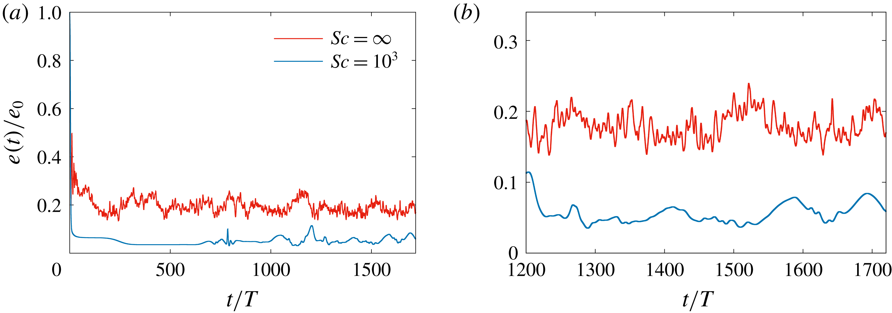
Figure 2 shows the time series of the kinetic energy
 $e(t)\equiv (1/2)\int _{V}|\boldsymbol{u}(\boldsymbol{x},t)|^{2}\,\text{d}\boldsymbol{x}$
. For
 $Sc=10^{3}$
, the system remains in an almost frozen state for a long time, after which it becomes chaotic. If the simulation is not long enough, such an initial frozen state may lead to a wrong interpretation of the dynamics, since the flow regime may be erroneously described as laminar. The behaviour of
 $e(t)$
is analogous to that found in Thomases & Shelley (Reference Thomases and Shelley2009) and Thomases et al. (Reference Thomases, Shelley and Thiffeault2011) for a four-roll mill force and same value of
 $Sc$
. For
 $Sc=\infty$
, in contrast, the motion of the solution becomes chaotic much more rapidly and, in the steady state, the kinetic energy fluctuates at a frequency much higher than when artificial diffusivity is present. Moreover, the mean kinetic energy is greater.
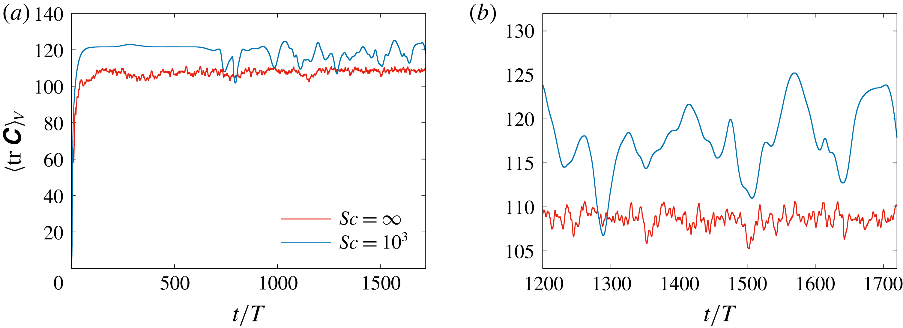
The time series of the trace of
 $\unicode[STIX]{x1D63E}$
averaged over
 $V$
show behaviours analogous to those of
 $e(t)$
, with
 $\langle \operatorname{tr}\unicode[STIX]{x1D63E}\rangle _{V}$
displaying much slower oscillations when
 $\mathit{Sc}=10^{3}$
and this only after a long, initial, almost frozen state (figure 3).
(a) Time series of the kinetic energy of the polymer solution rescaled by the kinetic energy of the fixed-point laminar flow (
 $\unicode[STIX]{x1D707}=0$
), i.e.
 $e_{0}\equiv f_{0}^{2}/2\unicode[STIX]{x1D708}^{2}K^{4}$
, for
 $Sc=\infty$
(red, top curve) and for
 $Sc=10^{3}$
(blue, bottom curve). (b) Zoom of (a) in the steady state.

(a) Time series of the trace of the polymer conformation tensor averaged over the spatial domain
 $V$
for
 $Sc=10^{3}$
(blue, top curve) and
 $Sc=\infty$
(red, bottom curve). (b) Zoom of (a) in the steady state.

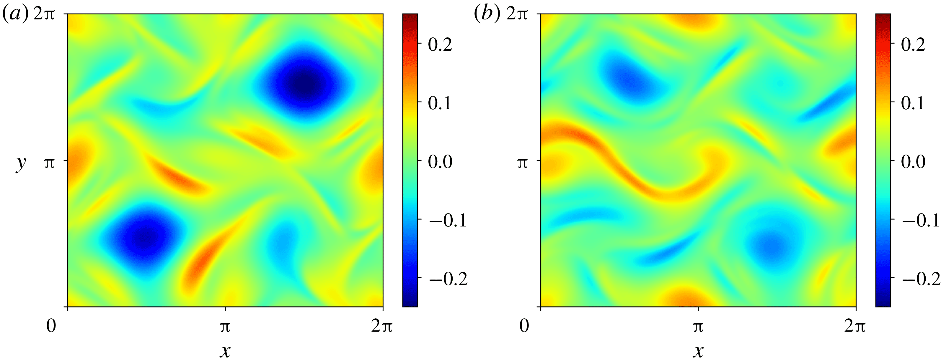
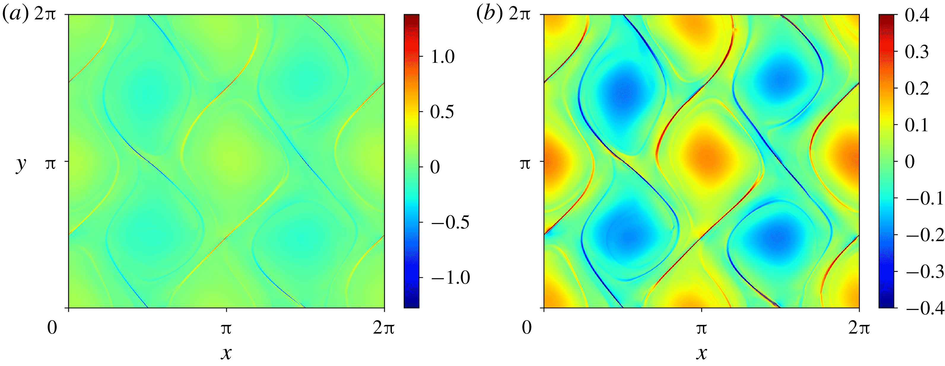
The snapshots of the vorticity field also indicate a striking difference between the two integration methods (figures 4 and 5). With artificial diffusivity, once the system starts fluctuating the spatial structure of the flow departs from that which would be imposed by the force (figure 4). Only some of the vortical cells continue to exist, whilst others break down and patches of vorticity contaminate the cellular structure of the base flow. Furthermore, the number and the location of unbroken vortical cells vary in time (see the snapshots at two different times in figure 4). This dynamics is equivalent to the symmetry-breaking transition observed by Thomases & Shelley (Reference Thomases and Shelley2009) and Thomases et al. (Reference Thomases, Shelley and Thiffeault2011). In contrast, for
 $Sc=\infty$
the vorticity field displays fluctuations which perturb the cellular vortices, but its large-scale structure essentially remains slaved to that of the background force (see figure 5 for a representative snapshot). Large perturbations of the vorticity field are concentrated on thin filaments located in the vicinity of the lines of pure strain which separate the vortical cells. Thus, the symmetry breaking shown in figure 4 is a spurious effect due to artificial diffusivity.
Snapshots of the vorticity field for
 $Sc=10^{3}$
at
 $t/T=1200$
(a) and
 $t/T=2212$
(b).

(a) A representative snapshot of the vorticity field for
 $Sc=\infty$
. (b) The same snapshot as in (a) but with a rescaled colour bar. The purpose of this rescaling is to show the cellular structure of the flow more clearly.

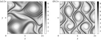
The snapshots of
 $\operatorname{tr}\unicode[STIX]{x1D63E}$
also show a strong qualitative difference in the behaviour of the polymer stress (figure 6). The analysis of these snapshots allows us to understand the effect of artificial diffusivity. Rather than the Schmidt number, here the relevant dimensionless parameter is the Péclet number
 $Pe=f_{0}/\unicode[STIX]{x1D705}\unicode[STIX]{x1D708}K^{3}$
, which is the ratio of the time scale associated with polymer-stress diffusion,
 $(\unicode[STIX]{x1D705}K^{2})^{-1}$
, and the time scale at which the polymer stress is convected,
 $T$
. When
 $\mathit{Sc}=\infty$
,
 $\mathit{Pe}$
is also infinite and the evolution of the polymer stress is dominated by convection. In this case, highly stretched polymers – and hence large polymer stresses – are essentially found in strain-dominated regions of the flow, while the polymer stress is weak in vortical regions, where polymers rapidly contract. Thus, in the cellular flow, the vorticity field is strongly affected by polymer stresses at the boundaries of the cells; inside the cells, the external force dominates and imposes the cellular structure. However, when polymer-stress diffusion becomes relevant (i.e.
 $\mathit{Sc}=10^{3}$
and, with our choice of parameters,
 $\mathit{Pe}=10^{3}$
), large polymer stresses spread far from the straining lines where they are created and reach the interior of the vortices; this destabilizes the cellular structure and generates the symmetry breaking observed at
 $Sc=10^{3}$
. Furthermore, we note that although for
 $Sc=\infty$
polymers can locally be highly stretched (figure 6), the average polymer stretching is generally higher for
 $Sc=10^{3}$
than for
 $Sc=\infty$
(figure 3).
Hameduddin et al. (Reference Hameduddin, Meneveau, Zaki and Gayme2018) recently proposed to quantify the deviation of the polymer configuration from the equilibrium one by considering the geodesic distance between
 $\unicode[STIX]{x1D63E}$
and
 $\unicode[STIX]{x1D644}$
in the space of positive-definite tensors. The snapshots of this distance (see the supplementary material) confirm the behaviours observed in the snapshots of
 $\operatorname{tr}\unicode[STIX]{x1D63E}$
(figure 6).


Figures 4 and 5 also indicate that the vorticity field is much smoother for
 $Sc=10^{3}$
than for
 $Sc=\infty$
. This can be understood by noting that, in elastic turbulence, the small scales of the flow are not activated by a cascade phenomenon but rather by the fluctuations of the polymer feedback at the same scales, and for
 $\mathit{Sc}=10^{3}$
the high-wavenumber fluctuations of the polymer stress are damped by diffusivity. The smoothness of the flow can be quantified by examining the spectrum of the velocity fluctuations,
 $E(k)\equiv \sum _{k-1/2<k^{\prime }\leqslant k+1/2}\langle |\hat{\boldsymbol{v}}(\boldsymbol{k}^{\prime },t)|^{2}\rangle _{t}$
, where
 $\langle \boldsymbol{\cdot }\rangle _{t}$
denotes the time average over the steady state and
 $\hat{\boldsymbol{v}}(\boldsymbol{k},t)$
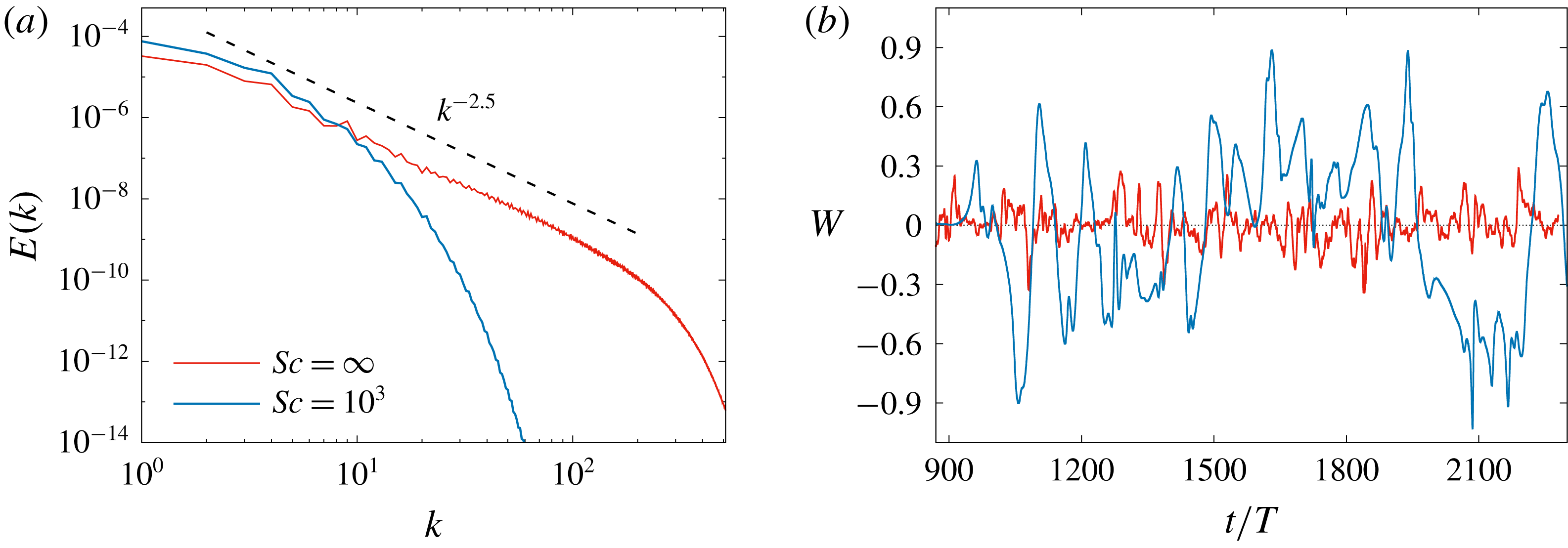
is the Fourier transform of the velocity field minus its time average. We find again that artificial diffusivity has a strong impact on the flow (figure 7
a). For
 $Sc=10^{3}$
,
 $E(k)$
decays very rapidly with the wavenumber, whereas for
 $Sc=\infty$
it behaves as a power law:
 $E(k)\propto k^{-2.5}$
. Thus, fluctuations are sustained at much smaller scales when
 $Sc=\infty$
. The power law is shallower than those found previously in experiments and numerical simulations with different forcings, in which the exponent varied with the set-up but was always smaller than
 $-3$
(Groisman & Steinberg Reference Groisman and Steinberg2000, Reference Groisman and Steinberg2004; Berti et al.
Reference Berti, Bistagnino, Boffetta, Celani and Musacchio2008; Ray & Vincenzi Reference Ray and Vincenzi2016; Watanabe & Gotoh Reference Watanabe and Gotoh2013, Reference Watanabe and Gotoh2014; Gupta & Pandit Reference Gupta and Pandit2017). A kinetic energy spectrum steeper than
 $k^{-3}$
was also predicted by Fouxon & Lebedev (Reference Fouxon and Lebedev2003). This prediction, however, does not necessarily apply to the case under consideration, because it assumes statistical homogeneity and isotropy and our flow does not enjoy these statistical symmetries. (Note that, for the Kolmogorov force, the same integration scheme used here yields the exponent
 $-3.7$
(Plan et al.
Reference Plan, Gupta, Vincenzi and Gibbon2017), which agrees with the results of Berti et al. (Reference Berti, Bistagnino, Boffetta, Celani and Musacchio2008); see also Berti & Boffetta (Reference Berti and Boffetta2010) and Garg et al. (Reference Garg, Calzavarini, Mompean and Berti2018).)
(a) Kinetic energy spectrum for
 $Sc=10^{3}$
and
 $Sc=\infty$
. For
 $Sc=\infty$
the spectrum behaves as the power law
 $k^{-2.5}$
. (b) Time series of
 $W$
. For
 $Sc=10^{3}$
,
 $W$
displays much larger fluctuations than for
 $Sc=\infty$
.

To quantify the breaking of the cellular symmetry, we also consider the ratio
 $$\begin{eqnarray}W={\displaystyle \frac{\unicode[STIX]{x1D714}(0,0)-\unicode[STIX]{x1D714}(\unicode[STIX]{x03C0},0)}{\unicode[STIX]{x1D714}(0,0)+\unicode[STIX]{x1D714}(\unicode[STIX]{x03C0},0)}},\end{eqnarray}$$
which compares the amplitude of vorticity at two positions in the flow,
 $(x,y)=(0,0)$
and
 $(x,y)=(\unicode[STIX]{x03C0},0)$
. For the laminar solution (
 $\unicode[STIX]{x1D707}=0$
), these two positions are the centres of two equal-sign vortices and
 $W=0$
. Non-zero values of
 $W$
therefore correspond to deviations from the cellular symmetry. Figure 7(b) shows that the fluctuations of
 $W$
are much larger for
 $Sc=10^{3}$
than for
 $Sc=\infty$
(analogous results are found for other couples of equal-sign vortices). This confirms that the cellular structure is strongly modified by artificial diffusivity.
4 Conclusions
In numerical simulations of constitutive models of polymer solutions the addition of artificial diffusivity is a well-known strategy for overcoming the numerical instabilities generated by the loss of positive definiteness of the polymer stress tensor. We have studied the accuracy of this approach in elastic turbulence by comparing simulations of the two-dimensional Oldroyd-B model sustained by a cellular external force, with and without artificial diffusivity. Our results show that artificial diffusivity has a strong impact on the qualitative spatial and temporal properties of the flow. In particular, with artificial diffusivity the cellular structure imposed by the external force breaks down, as also found by Thomases & Shelley (Reference Thomases and Shelley2009) and Thomases et al. (Reference Thomases, Shelley and Thiffeault2011) for a four-roll mill force and the same value of
 $Sc$
. Without artificial diffusivity, the flow is mainly perturbed in strain-dominated regions but, albeit chaotic, essentially reproduces the symmetries of the background force.
We have also performed simulations of the FENE-P model in exactly the same setting and found similar results (see appendix A); hence the effect of artificial diffusivity is not modified by the nonlinearity of the elastic force.
To preserve the positive definiteness of the polymer conformation tensor and to accurately resolve its gradient, we have used a combination of the Cholesky decomposition and the Kurganov–Tadmor hyperbolic solver. Adding artificial diffusivity to this scheme produces the migration of high polymer stresses to regions of the flow where in principle polymers would be weakly stretched. This generates strong differences in the large-scale flow. We believe that this effect of artificial diffusivity is not specific to the Kurganov–Tadmor scheme, i.e. the addition of an excessively large polymer-stress diffusion is expected to produce analogous modifications of the large-scale flow also in other integration schemes and, vice versa, if a scheme does not use artificial diffusivity or similar dissipation terms, it should not produce the symmetry breaking discussed above.
We have described the motion of the fluid by means of the Stokes equations, as in some of the previous studies on elastic turbulence. Other studies have used the Navier–Stokes equations. Thus, we have also performed numerical simulations of (2.1b
) coupled with the Navier–Stokes equations with the same cellular force. The Reynolds number
 $Re=f_{0}/\unicode[STIX]{x1D708}^{2}K^{3}$
has been set to unity, which is below the critical value for the appearance of inertial instabilities,
 $Re_{c}=\sqrt{2}$
(Gotoh & Yamada Reference Gotoh and Yamada1984). The conclusions on the effect of artificial diffusivity are exactly the same as when the Stokes equations are used.
In our study, we specifically selected the cellular force in order to illustrate the impact of artificial diffusivity on numerical simulations of elastic turbulence. This force indeed generates a flow in which the straining and vortical regions are distinct. Hence in the absence of artificial diffusivity the polymer stress is chiefly located at the straining regions, whereas in the presence of diffusivity it spreads outside them. For other external forces that mix strain and vorticity, the effect of artificial diffusivity may be less dramatic. This is the case, for instance, of the Kolmogorov force, which in the absence of polymer feedback and at low Reynolds numbers generates a sinusoidal shear. For the Kolmogorov force, the velocity spectrum indeed behaves as a power law even for
 $Sc=10^{3}$
(Garg et al.
Reference Garg, Calzavarini, Mompean and Berti2018), although of course the power law is observed on a smaller range of wavenumbers compared to simulations that do not use artificial diffusivity (Plan et al.
Reference Plan, Gupta, Vincenzi and Gibbon2017).
The effect of artificial diffusivity is more dramatic in elastic turbulence than at high Reynolds numbers or in laminar flows. In these latter cases, indeed, artificial diffusivity produces quantitative changes in the solution of the Oldroyd-B and FENE-P models but does not modify the qualitative behaviour of the velocity and polymer conformation fields, provided of course
 $Sc$
is not excessively small (see, e.g., figures 8–10 in Vaithianathan et al.
Reference Vaithianathan, Robert, Brasseur and Collins2006 and figures 3 and 4 in Sid et al.
Reference Sid, Terrapon and Dubief2018 for the high-Reynolds-number regime and figure 7 in Thomases Reference Thomases2011 for the laminar regime). In elastic turbulence, before the addition of polymers the flow is laminar. Artificial diffusivity thus strongly modifies the large-scale flow by bringing high polymer stresses to regions of the fluid where the polymers would be weakly stretched and hence the flow would be weakly chaotic. This effect is peculiar to the regime of elastic turbulence and can lead to the spurious behaviours described above. Therefore, great caution should be taken in using artificial diffusivity to prevent numerical instabilities in simulations of elastic turbulence.
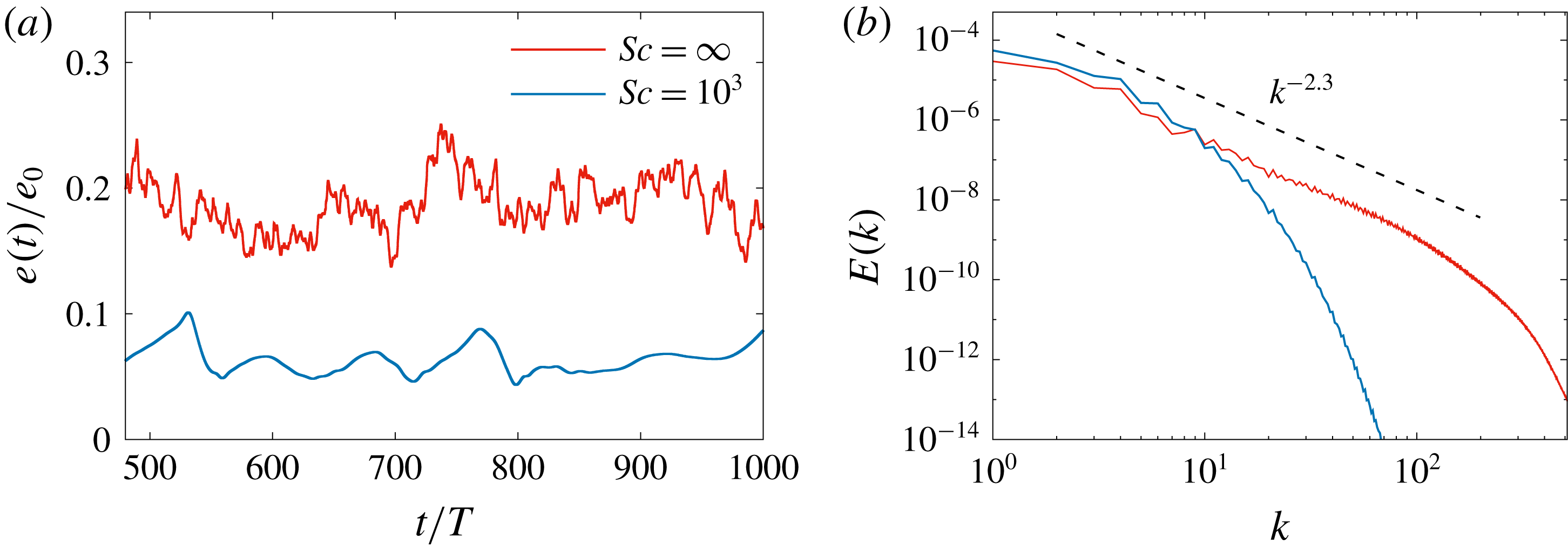
FENE-P model. (a) Time series of the rescaled kinetic energy in the steady state for
 $Sc=\infty$
(red, top curve) and
 $Sc=10^{3}$
(blue, bottom curve). (b) Kinetic energy spectra for
 $Sc=10^{3}$
and
 $Sc=\infty$
. For
 $Sc=\infty$
the spectrum behaves as the power law
 $k^{-2.3}$
.

Acknowledgements
We would like to thank T. Matsumoto for useful discussions. The computations were performed at Centre de Calcul Interactif, Université Nice Sophia Antipolis and Mésocentre SIGAMM, Observatoire de la Côte d’Azur.
Supplementary material
Supplementary material is available at https://doi.org/10.1017/jfm.2019.224.
Appendix A. Effect of artificial diffusivity in the FENE-P model
A drawback of the Oldroyd-B model is that there is not a maximum polymer extension. Infinitely large extensions are in principle allowed, and in certain flow conditions
 $\operatorname{tr}\unicode[STIX]{x1D63E}$
grows indefinitely. In the FENE-P model, a maximum polymer extension
 $\ell _{max}$
is imposed by modifying (2.1) as follows:
 $$\begin{eqnarray}\displaystyle & \displaystyle \unicode[STIX]{x1D735}p=\unicode[STIX]{x1D708}\unicode[STIX]{x0394}\boldsymbol{u}+{\displaystyle \frac{\unicode[STIX]{x1D707}}{\unicode[STIX]{x1D70F}}}\,\unicode[STIX]{x1D735}\boldsymbol{\cdot }[h(\operatorname{tr}\unicode[STIX]{x1D63E})\unicode[STIX]{x1D63E}]+\boldsymbol{f},\qquad \unicode[STIX]{x1D735}\boldsymbol{\cdot }\boldsymbol{u}=0, & \displaystyle\end{eqnarray}$$
 $$\begin{eqnarray}\displaystyle & \displaystyle \unicode[STIX]{x2202}_{t}\unicode[STIX]{x1D63E}+\boldsymbol{u}\boldsymbol{\cdot }\unicode[STIX]{x1D735}\unicode[STIX]{x1D63E}=(\unicode[STIX]{x1D735}\boldsymbol{u})\boldsymbol{\cdot }\unicode[STIX]{x1D63E}+\unicode[STIX]{x1D63E}\boldsymbol{\cdot }(\unicode[STIX]{x1D735}\boldsymbol{u})^{\top }-{\displaystyle \frac{h(\operatorname{tr}\unicode[STIX]{x1D63E})\unicode[STIX]{x1D63E}-\unicode[STIX]{x1D644}}{\unicode[STIX]{x1D70F}}}, & \displaystyle\end{eqnarray}$$
 $$\begin{eqnarray}h(\unicode[STIX]{x1D701})={\displaystyle \frac{\ell _{max}^{2}-2}{\ell _{max}^{2}-\unicode[STIX]{x1D701}}}.\end{eqnarray}$$
The function
 $h(\operatorname{tr}\unicode[STIX]{x1D63E})$
diverges as
 $\operatorname{tr}\unicode[STIX]{x1D63E}$
approaches
 $\ell _{max}^{2}$
and hence causes
 $\operatorname{tr}\unicode[STIX]{x1D63E}$
to stay smaller than
 $\ell _{max}^{2}$
.
In this appendix, we report simulations of the FENE-P model with and without artificial diffusion. The maximum polymer square extension is
 $\ell _{max}^{2}=3\times 10^{3}$
, while the other parameters of the FENE-P model are the same as those used for the Oldroyd-B model in § 3. Equation (A 1b
) is solved by combining the Cholesky decomposition and the Kurganov–Tadmor hyperbolic solver as described in § 2. The effect of artificial diffusivity is once again studied by adding the term
 $\unicode[STIX]{x1D705}\unicode[STIX]{x0394}\unicode[STIX]{x1D63E}$
with
 $\unicode[STIX]{x1D705}=5\times 10^{-5}$
to (A 1b
), so that
 $\mathit{Sc}=10^{3}$
. Figures 8 and 9 are the counterparts for the FENE-P model of figures 2(b), 6(a) and 7(a). The results show that the conclusions on the effects of artificial diffusivity obtained for the Oldroyd-B model hold analogously for the FENE-P model.
FENE-P model: representative snapshots of
 $\ln (\operatorname{tr}\unicode[STIX]{x1D63E})$
in the steady state for
 $Sc=10^{3}$
(a) and
 $Sc=\infty$
(b).