

Introduction
It is well established that increasing socioeconomic status (SES) has a beneficial effect on health and longevity. This is generally true irrespective of how SES is measured. In the Whitehall I study of British civil servants, Marmot and colleagues reported that men of lower employment grades had higher blood pressure, higher glucocorticoids in the bloodstream and less leisure-time physical activity than men of higher employment grades (Marmot et al., 1978a, b; Marmot et al., Reference Marmot, Shipley and Rose1984). The subsequent Whitehall II study supported these findings while providing more information about causal factors (Marmot et al., Reference Marmot, Stansfeld, Patel, North, Head, White and Smith1991). Men of lower employment grades were found to have lower job satisfaction and autonomy at work than their superiors. These variables have been linked to cardiovascular problems in other studies through their contribution to psychosocial stress. Moreover, many other studies have similar findings about socioeconomic status and health. These include The Black Report on the effects of occupation (Black et al., Reference Black, Townsend and Davidson1982), studies on the specific effect of income (Ettner, Reference Ettner1996; Kawachi & Kennedy, Reference Kawachi and Kennedy1999; Lynch et al., Reference Lynch, Smith, Kaplan and House2000; Marmot, Reference Marmot2002), and studies regarding the myriad pathways linking education to health and mortality (Comstock & Tonascia, Reference Comstock and Tonascia1977; Bourne & Walker Jr, Reference Bourne and Walker1991; Kunst & Mackenbach, Reference Kunst and Mackenbach1994; Ross & Wu, Reference Ross and Wu1995; Son et al., Reference Son, Armstrong, Choi and Yoon2002; Mirowsky & Ross, Reference Mirowsky and Ross2003; Malyutina et al., Reference Malyutina, Bobak, Simonova, Gafarov, Nikitin and Marmot2004).
Questions remain, however, about how this association may be attenuated or enhanced based on predisposing susceptibilities or protective factors suggested by an individual's family medical history. An important but generally neglected element in social disparities research is family history of longevity. Numerous studies conducted over the last century by biologists, population geneticists, evolutionists and demographers have examined the familiality of longevity (Beeton et al., Reference Beeton, Yule and Pearson1900; Beeton & Pearson, Reference Beeton and Pearson1901; Pearl, Reference Pearl1931; Williams, Reference Williams1957; Abbott et al., Reference Abbott, Abbey, Bolling, Murphy and Opitz1978; Philippe & Opitz, Reference Philippe and Opitz1978; Wyshak, Reference Wyshak1978; Vaupel, Reference Vaupel1988; Bocquet-Appel & Jakobi, Reference Bocquet-Appel and Jakobi1990; McGue et al., Reference McGue, Vaupel, Holm and Harvald1993; Carmelli et al., Reference Carmelli, Swan and Cardon1995). Reported heritability estimates of age at death vary widely, ranging from nearly zero to 0.33, in part because of differences in the types of paired relationships examined, the time periods and number of generations considered, and the quality of data among source populations. These estimates are normally derived from familial correlations. Accordingly, they may be elevated by shared environmental factors, but that vary within and between populations. Recent studies using the Utah Population Database (UPDB), however, indicate that a strong association exists between mortality and a specific operationalization of family history of longevity that emphasizes genetic relations between blood relatives (Kerber et al., Reference Kerber, O'Brien, Smith and Cawthon2001; Smith et al., Reference Smith, Mineau, Garibotti and Kerber2009).
While there is no dispute that a strong familial predisposition for longer life will enhance an individual's own chances of better survival, not all such individuals benefit equally from this protective influence. The concern here is whether a critical environmental social influence, SES, modifies the survival benefits of a family history of longevity. The nature of this interaction is complex and increasing SES may conceivably work to amplify or attenuate the way in which familial longevity alters individual risks of mortality. What are the possible mechanisms by which these interactions could occur? One possibility is that individuals with a better familial longevity history are more immune to serious health problems suffered disproportionately by those with low SES. In this case, the relative survival benefits of having a beneficial longevity heritage would be greater for people from low SES backgrounds than for those with high SES. However, it is also plausible that mortality among high SES persons is more sensitive to familial excess longevity since many of the health benefits attributable to having long-lived ancestors may be difficult to experience without access to resources (e.g. higher levels of education, knowledge about preventive health behaviours) that promote better survival prospects.
The purpose of this analysis is to address the questions of whether and how SES and familial longevity interact by examining the male mortality risks after age 40 for men born from 1840 to 1909. It uses data from the Utah Population Database (UPDB), which is used to generate measures of family history of longevity and SES, years of life lived past age 40, and additional variables necessary to adjust for potential confounding factors.
Methods
Data
The analyses are based on the UPDB, one of the world's largest and most comprehensive computerized population-based genealogies linked to health and vital records. In the 1970s, approximately 170,000 Utah nuclear families were identified on ‘Family Group Sheets’ from the archives at the Utah Family History Library, each with at least one member having had a vital event (birth, marriage, death) on the Mormon Pioneer Trail or in Utah. These families have been linked across generations; in some instances, the records span twelve generations. The UPDB records provide data on migrants to Utah and their Utah descendants that number more than 1.6 million individuals born from the early 1800s. The UPDB includes individuals who have lived in other states and countries and describes families with and without an affiliation to the Church of Jesus Christ of Latter-day Saints (LDS or Mormons). The UPDB is actively creating family histories: new families and their members are continually added as the UPDB is linked to other sources of data, including birth and death certificates. Additional information on these families comes from sources such as driver license records and the Utah Cancer Registry. Because these records include basic demographic information on parents and their children, fertility and mortality data are extensive with coverage up to 2010.
In this study, data were used from the UPDB that are ideally suited to the research question. First, the analysis was focused on men because, for the time period used and region covered by the data set, men were much more likely to be employed in an occupation and, therefore, would have data available about that occupation and where they would experience its potential health effects most directly. It was necessary to select an extinct cohort because death certificates provided both death dates (as did genealogies within the UPDB) along with occupation and industry information used to derive an SES measure. Men aged 40 or over at the time of death were exclusively studied because younger men would not have generally achieved their full occupational status at younger ages and the mortality risk from stress and resource-related diseases would be less likely to occur before age 40. Married men were used to the exclusion of non-married men since marriage is a necessary condition for an individual to have a measure of spouse excess longevity, a variable that is described in more detail below. Arguably, the restriction to include married men only does not represent a significant bias given that the overwhelming majority of men age 40 and over living in Utah during the study period had been married. Furthermore, while it is plausible that the never-married men that were excluded experienced higher mortality at younger ages than married men, there is no reason to expect that this would substantially influence the relationship between mortality and the predictor variables used in the analysis.
Measures
Mortality
For the hazard rate models, the outcome is the hazard rate for all-cause mortality starting at age 40.
Socioeconomic status (SES)
The measure of SES used here is the Nam and Powers (Nam & Powers, Reference Nam and Powers1983) index of occupational status. They calculate SES as the average of the median income and median educational level of people who work at a specific occupation. The list of occupations used by these authors is the detailed occupational list created for the 1970 US Census, which provides the benefit of grouping occupations so that there is a large degree of homogeneity with regard to occupational characteristics. The procedure they use for calculating the occupational status scores involves (a) arraying the occupations according to the median educational level of those working at them; (b) arraying the same occupations separately according to the median income level of those working at them; (c) by using the number of persons engaged in each occupation, determining the cumulative interval of people in each occupation for each of the two arrays, beginning with the lowest-ranked occupation; and (d) averaging the midpoints of the two cumulative intervals of persons in each occupation and dividing by the number of persons in the workforce to get a status score for the occupation. Using 1970 US Census data, Nam and Powers calculated separate scores for male and female occupants. The resulting occupational status scores span 0 and 100, and a given score indicates the approximate percentage of persons in the workforce in 1970 that were in occupations having combined average levels of median education and income below that for the given occupation.
A dummy variable was introduced for whether or not a subject's Nam–Powers SES represented farming (i.e. a Nam–Power score of 40). This is justified on the basis that a very large proportion of men in the data set were farmers (35.5%), the single largest occupation group in the sample. This is not surprising given the years covered in this sample. Using this dummy variable allows the analysis to control for the effects of being a farmer on survival and examine it separately from the general effects of SES.
The Nam–Powers score adopted here may be subject to a minimal level of measurement error since it was based on the occupational structure in 1970. The median year of death was approximately 1960 so some men who died earlier in time might have occupations that may not optimally map to the 1970 schema. This problem was partially mitigated by the fact that a large fraction (35%) were farmers, an occupation less subject to measurement error. (Nevertheless, even within that occupation a degree of variation probably exists, reflecting changes in the structure of the agriculture industry over the duration included in the data set.)
Familial excess longevity (FEL)
Familial excess longevity is a measure of an individual's history of longevity among his or her blood relatives (Kendler et al., Reference Kendler, Kessler, Walters, MacLean, Neale, Heath and Eaves1995). To construct FEL, the analyses rely on a measure of individual-level excess longevity: the difference between an individual's attained age y and the age that that individual was expected to live based on a model that incorporates two fundamental factors affecting survival, gender and birth year. Expected longevity, y*, is estimated from an accelerated failure time model and excess longevity is y−y*, where y is the attained age either at death or at the time last confirmed the subject was alive. To generate FEL, only persons who reached the age of 65 were included so that the measure is based on those whose death was less likely to arise from external causes. This excess longevity measure is then extended to all blood relatives living to at least age 65 for each man in the sample. Averaging the excess longevities of all such relatives for each man, weighted by their kinship coefficient, generates a point estimate of FEL. The kinship coefficient is the probability that an individual shares a particular allele with another individual identical by descent from a common ancestor. Generally, each man in the sample has hundreds of kin who lived to age 65 on whom their FEL measure was based.
Spousal excess longevity (SEL)
To control indirectly for environmental factors contributing to longevity, the spousal excess longevity (SEL) measure is employed (Kerber et al., Reference Kerber, O'Brien, Smith and Cawthon2001). Spousal excess longevity, like FEL, is the average excess longevity among the spouses of a subject's relatives (again for blood relatives living to age 65), weighted by the kinship coefficient of the relatives. If a man has more than one spouse, only the first is used. Spousal excess longevity is based on the idea that a positive family history of longevity may arise because of an advantageous environment that can be detected by assessing the longevity of those married to an individual's relatives.
Religiosity
For this population, members active in the LDS Church may benefit from their religious participation in terms of longevity as well as SES. The UPDB contains the dates of two significant religious events for Mormons: baptism and endowment. Baptism typically occurs when a Mormon reaches his or her eighth birthday or later if they convert to the faith. Baptisms are treated as an indicator of the faith in which the child was reared. Endowment, on the other hand, normally occurs in early adulthood, requires that a person has already been baptized, signifies a deeper commitment to the Church, and is an explicit pledge on the part of the individual to follow the tenets of the religion. For this study, men who have been baptized (typically by age eight) but not endowed are classified as ‘inactive’, and those who have been endowed as ‘active’. Persons without a baptism or endowment date are categorized as being a non-Mormon. Each of these measures is represented by a dichotomous dummy variable. These measures of religiosity are included to control for health-related behaviour, as Mormons are less likely to use alcohol and tobacco and are more likely to participate in church and religious activities than are non-Mormons.
Urbanicity
Mortality risks are affected by geography and here the role of living in an urban or rural setting is considered. The analysis controls for whether men lived in an urban or rural area using a dichotomous variable for urban versus rural. The UPDB contains data on county of death, which was the basis for classifying the county by their urbanicity. The four counties of Salt Lake, Utah, Weber and Davis are defined as urban counties during the time period covered by the study. While some deceased men in the data set undoubtedly moved between urban and rural areas after retirement, it is unlikely that this represents a substantial bias for this control variable or influenced the relationship between mortality age and the predictor variables.
Age at baseline
The data used include men born between 1840 and 1910, but the authors have death certificates (from which SES information was derived) beginning in 1904. Accordingly, the data set does not include data on men at age 40 for those born from 1840 to 1863. To address this feature of the data in the analysis, the authors control for the earliest age at which death is measured, and for which a male may appear in the data set.
Analysis
All models are based on Cox proportional hazards regression (PHM) or logistic regression. With the Cox PHM, time between age 40 and death is modelled. These models generate estimates of the effects of the independent variables on the hazard rate of all-cause mortality. A general form of the PHM for this analysis is:
 $$h_i ({\alpha})=h_0({\alpha}) {\rm exp} ({\beta}_1 {\rm FEL}+{\beta}_2{\rm SES}+ {\beta}_3 ({\rm FEL} \times {\rm SES}) + \cdots+ {\beta}_k\times X_k$$
where i indexes individuals, a measures age, FEL is familial excess longevity and SES is the Nam–Powers socioeconomic score, FEL×SES is the key interaction variable, the X values are additional covariates described previously (including SEL) and β values are unknown regression parameters. Consistent with the literature, it is expected that higher levels of SES and FEL will be associated with lower mortality hazard rates (i.e. β 1, β 2<0). Importantly, it is also expected that higher levels of both SES and FEL jointly will be associated with an additional protective effect on mortality (i.e. β 3<0).
Three distinct models are estimated. The first Cox PHM estimates the main effects of SES and FEL along with controlling for key potential confounders such as environmental factors and health-related behaviour, as described above. This model makes the distinction between SES across the full range of the Nam–Powers score as well as a dummy variable for whether the individual was a farmer. The second model then includes the interaction between SES and FEL as well as between being a farmer and FEL. The third model trichotomizes SES into whether a male subject attained the top 15th percentile, the middle 70% or the bottom 15th percentile; the latter category is the reference category. The two SES dummy variables are included (in lieu of the interval-level SES) along with the farmer dummy and their interactions with FEL. This operationalization allows us to show how men at the extremes in SES fare and how these large differences in SES affect survival by FEL.
The logistic regression models are used to estimate the effects of the SES, FEL and their interaction on the odds of surviving to the top 5th percentile in life span. These models are expressed as follows:
 $$Ln(Pr{Living to the 95 pct})/(1-Pr{Living to the 95 pct})=\beta_0+\beta_1 {FEL}+\beta_2 {SES}+\beta_2 ({FEL}\times SES)+\cdots+\beta_k X_k$$
where i indexes individuals, β 0 is the intercept, FEL and SES are the main covariates, FEL×SES is the interaction variable, X values are additional covariates and βj are the j regression parameters to be estimated. Comparable to our hypotheses applied in the survival analysis, these variables should be positively associated with the odds of surviving to the top 5th percentile in age (i.e. β 1, β 2, β 3>0).
Results
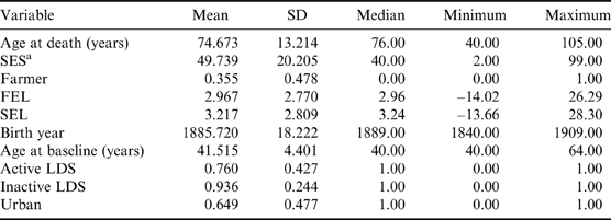
Descriptive statistics for all variables used in the models are shown in Table 1. Several features of the data merit comment. First, the distribution for SES is positively skewed. This is due to the high proportion of farmers with a score of 40, which reduces the mean and the median. Second, the mean for the FEL variable is 2.97 years. This figure indicates that men have blood relatives who live approximately 3 years longer (rather than zero) than expected. For the full UPDB, the mean FEL equals zero. This feature of the data is a function of the survival selection imposed on this sample where all men survived to at least the age of 40.
Descriptive statistics for variables, men born between 1840 and 1909, Utah Population Database

a Nam–Powers index.
N for all variables=90,700.
Cox proportional hazards models
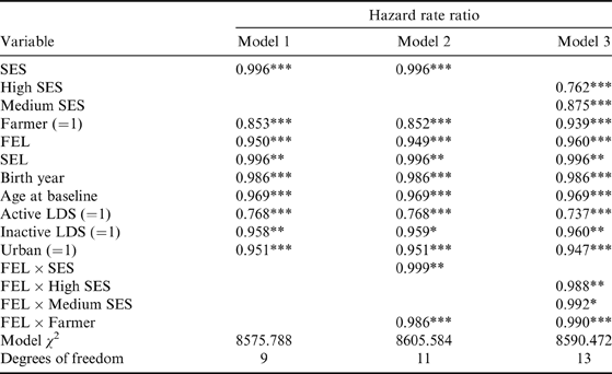
The hazard rate ratios (HRRs) for the Cox PHMs are displayed in Table 2. For Model 1, the HRRs indicate that increasing levels of SES, as well as being a farmer, reduces the risk of mortality. For a ten-unit increase in the Nam–Powers score, men's mortality hazard declines by 4%; and the mortality hazard for farmers is 15% lower than non-farmers. The mortality hazard decreases by 5% for every one-unit (i.e. one year) increase in FEL. The protective effects of increasing values of SEL are also significant though its absolute size is considerably smaller than it is for FEL. These mortality effects are significant after controlling for birth year, region and health-related behaviour.
Hazard rate ratios from Cox proportional hazards models for the hazard of all-cause mortality, with interaction effects between socioeconomic status (SES) and familial excess longevity (FEL)
All model χ2 values are significant at p<0.001.
*p<0.05; **p<0.01; ***p<0.001.
Model 2 shows that the interactions between FEL with SES, as well as the interaction with the farmer dummy variable, are statistically significant. In general, the interaction indicates that the protective effects of increasing SES are enhanced with rising values of familial longevity. In addition, increasing FEL is associated with reduced mortality risks, an association that increases with higher SES values.
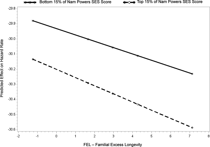
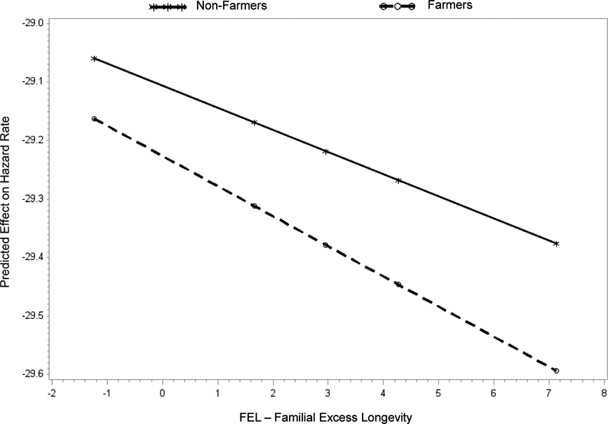
The interaction between SES and FEL, as well as the interaction between the farmer dummy and FEL, can be better represented graphically. Two plots are represented using a categorized SES where the top and bottom 15th percentiles are compared. A representation of these interactions can be seen in Figs 1 and 2. Figure 1, based on Model 3, shows that as FEL increases, the mortality hazard decreases more precipitously for men in the top 15th percentile in SES than for men in the bottom 15th percentile. Specifically, Model 3 indicates that the mortality hazard among men in the top 15th percentile decreases 1.2% more for every one-unit increase in FEL than it does among men in the bottom 15th percentile (p<0.01). Figure 2, based on Model 2, shows that the differential effects of FEL are also present between farmers and non-farmers. The mortality hazard for farmers decreases 1.4% more for every one-unit increase in FEL than it does for non-farmers (p<0.001).
Effect of FEL within categories of SES.
Effect of FEL within categories of Farmer.
Whether the joint beneficial aspects of having a familial longevity history and higher SES may be detectable when examining causes of death with strong familial elements (cardiovascular disease), as opposed to causes lacking this quality (accidents), was also considered. Accordingly, competing risks Cox models were estimated that considered these two broad classes of death. Indeed, the advantageous interaction effects of higher SES/farming with increasing levels of FEL were detected for mortality from cardiovascular disease and not from accidental deaths (results not shown). The effect of SEL, as a marker for adversity in the environment, as a main effect, is significant for accidental mortality risk but not for cardiovascular mortality.
Logistic regression models
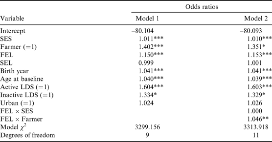
Odds ratios for the logistic regression models are shown in Table 3. Model 1 indicates that SES, being a farmer and FEL are all positively associated with surviving to the top 5th percentile in longevity (93 years of age and above). The odds of living to this advanced age for men increases by 1% for every one-unit increase in SES, 15% for every one-unit increase in FEL and is 40% higher among farmers than among non-farmers. Model 2 shows that no significant interaction exists between SES and FEL in affecting survival to the top 5th percentile. However, this model shows that there is indeed an interaction between being a farmer and one's FEL level. Every one-unit increase in FEL increases the odds that a farmer will survive to the top 5th percentile in longevity by 4.6% more than it does for non-farmers.
Odds ratios from logistic regression models of the log odds of surviving to the top 5th percentile in longevity, with interaction effects between socioeconomic status (SES) and familial excess longevity (FEL)
All model χ2 values are significant at p<0.001.
*p<0.05; **p<0.01; ***p<0.001.
Discussion
The findings of this study are consistent with the literature on the gradient between SES and longevity, FEL and longevity, and other research conducted on the UPDB identifying the protective effects of being a farmer. These results are statistically significant after controlling for environmental factors and health-related behaviour. Most notably, the analysis suggests that high-SES men and farmers benefit from having long-lived relatives more than low SES men and those who are not farmers.
What do farming and occupations reflective of high SES have in common that could explain this? It is likely that common features of these occupations responsible for decreased mortality are (1) the amount of physical activity a person gets, and (2) the amount of autonomy they are allowed. Both of these features are associated with lower rates of cardiovascular disease and mortality and, as noted in the literature on the SES–health gradient, both are characteristics of people with higher-grade occupations (Adler et al., Reference Adler, Boyce, Chesney, Cohen, Folkman, Kahn and Leonard1994; Marmot et al., Reference Marmot, Bosma, Hemingway, Brunner and Stansfeld1997; Hemingway et al., Reference Hemingway, Shipley, Brunner, Britton, Malik and Marmot2005). There is also reason to believe that the occupation of farming has historically imparted the same life-preserving benefits. During the time period examined, most farmers worked on family farms that existed before agglomeration resulted in the large modern farms in the United States presently (Lobao & Meyer, Reference Lobao and Meyer2001). Furthermore, since the data cover men who were farmers during the transition from an agricultural to industrial economy in Utah, it is possible that those whose death certificates listed them as farmers were successful and wealthy ones instead of those who would have found other employment.
But why do high-SES men and farmers benefit more from FEL than others? This question is best explored from the perspective of the literature on gene–environment (GE) interactions. Since the analysis controls for SEL and other environmental factors as much as the historic data allow, FEL is a genetic variable that does not include the benefits of a shared environment. In a review of the GE literature, Shanahan & Hofer (Reference Shanahan and Hofer2005) created a typology of GE interactions, including what they referred to as ‘contextual triggering’, describing a situation in which genotype and social context have an additive effect on the likelihood or intensity of the phenotype. More specifically, the analysis fits within the ‘stress diathesis model’ of contextual triggering, whereby ‘environmental stressors interact with personal predispositions to produce disease states, illness, and decrements of well-being’ (Shanahan & Hofer, Reference Shanahan and Hofer2005, p. 66). Other studies of this type include those on interactions between stressful life events and a genetic predisposition for depression (Kendler et al., Reference Kendler, Kessler, Walters, MacLean, Neale, Heath and Eaves1995; Silberg et al., Reference Silberg, Pickles, Rutter, Hewitt, Simonoff, Maes and Eaves1999; Beck, Reference Beck2008; Belsky & Pluess, Reference Belsky and Pluess2009; El Hage et al., Reference El Hage, Powell and Surguladze2009; Courtet et al., Reference Courtet, Gottesman, Jollant and Gould2011), while some examine adoptees in terms of how environment moderates genetic risk for a variety of psychological and behavioural conditions (Mednick et al., Reference Mednick, Gabrielli and Hutchings1984; Cutrona et al., Reference Cutrona, Cadoret, Suhr, Richards, Troughton, Schutte and Woodworth1994; Tienari et al., Reference Tienari, Wynne, Moring and Lahti1994; Cadoret et al., Reference Cadoret, Yates, Ed, Woodworth and Stewart1995; Hicks et al., Reference Hicks, South, DiRago, Iacono and McGue2009; Beaver, Reference Beaver2011; Wicks et al., Reference Wicks, Hjern and Dalman2010; Hakko et al., Reference Hakko, Wahlberg, Tienari and Räsänen2011).
More research using different data and control variables is needed to clarify the additive GE interaction between SES, farming and FEL, especially given the potential bias in the data used in this article introduced by the exclusion of unmarried men, a control variable for urban or rural habitation measuring location at death only and the use of temporally static socioeconomic status scores (which, perhaps most notably, do not distinguish between types of farmers). Still, the analysis here suggests that the benefits of FEL are indeed more available to those who engage in intense physical activity and have autonomy. Avoiding the excessive levels of glucocorticoids associated with lack of physical activity and autonomy may enable people with long-lived relatives to benefit from their healthy genes by putting off cardiovascular disease or other illnesses until later ages. Among those with lower SES, it appears plausible that the health benefits of having genes associated with long life become suppressed by a lack of physical activity and autonomy.
Acknowledgments
The authors are grateful to the Pedigree and Population Resource (funded by the Huntsman Cancer Foundation) for providing the data and valuable computing support. The study was supported by NIH grant AG022095 (The Utah Study of Fertility, Longevity, and Aging). The following individuals provided helpful comments on earlier drafts of this article: Alexandre Couture Gagnon, Steven Prus and Norm Waitzman.