2. Governing equations and numerical methodology

A set of reference scales are introduced to normalize the variables in compressible turbulence (Wang et al. Reference Wang, Shi, Wang, Xiao, He and Chen2012a,Reference Wang, Shi, Wang, Xiao, He and Chenb; Liang & Li Reference Liang and Li2013, Reference Liang and Li2015). The reference length $L_{\infty }$, free-stream velocity $U_{\infty }$, density $\rho _{\infty }$, pressure $p_{\infty }= \rho _{\infty }U_{\infty }^{2}$, free-stream temperature $T_{\infty }$, energy per unit volume $\rho _{\infty }U_{\infty }^{2}$, viscosity $\mu _{\infty }$ and thermal conductivity $\kappa _{\infty }$ are utilized. Thus, three non-dimensional governing parameters appear: the Reynolds number $Re= \rho _{\infty }U_{\infty }L_{\infty }/\mu _{\infty }$, the Mach number $M= U_{\infty }/c_{\infty }$ and the Prandtl number $Pr= \mu _{\infty } C_{p}/\kappa _{\infty }$. Ratio $\gamma = C_{p}/C_{v}$ is the ratio of specific heat at constant pressure $C_{p}$ to that at constant volume $C_{v}$, which is assumed to be equal to 1.4. The parameter $\alpha$ is defined as $\alpha = PrRe ( \gamma -1 )M^{2}$, where $Pr$ is assumed to be equal to 0.7.

The following dimensionless Navier–Stokes equations in conservation form are solved numerically (Wang et al. Reference Wang, Wan, Chen and Chen2018, Reference Wang, Wan, Chen, Xie, Zheng, Wang and Chen2020):

(2.1)$$\begin{gather} \frac{\partial \rho }{\partial t}+ \frac{\partial(\rho u_{j})}{\partial x_{j}}=0, \end{gather}$$

(2.2)$$\begin{gather}\frac{\partial ( \rho u_{i} )}{\partial t}+\frac{\partial [ \rho u_{i}u_{j}+p\delta _{ij} ]}{\partial x_{j}}=\frac{1}{Re}\frac{\partial \sigma _{ij}}{\partial x_{j}}, \end{gather}$$

(2.3)$$\begin{gather}\frac{\partial E}{\partial t}+\frac{\partial [ ( E+p )u_{j} ]}{\partial x_{j}}=\frac{1}{\alpha }\frac{\partial}{\partial x_{j}} \left( \kappa \frac{\partial T}{\partial x_{j}} \right) +\frac{1}{Re}\frac{\partial ( \sigma _{ij}u_{i} )}{\partial x_{j}}, \end{gather}$$

(2.4)$$\begin{gather}p=\rho T/( \gamma M^{2} ), \end{gather}$$

where $u_{i}$ is the velocity component, $\rho$ is the density, $p$ is the pressure and $T$ is the temperature. Parameter $\sigma _{ij}$ is the viscous stress and is defined as

(2.5)\begin{equation} \sigma _{ij}=\mu \left( \frac{\partial u_{i}}{\partial x_{j}}+\frac{\partial u_{j}}{\partial x_{i}} \right)-\tfrac{2}{3}\mu \theta \delta _{ij}, \end{equation}

where $\theta = {\partial u_{k}}/{\partial x_{k}}$ is the velocity divergence. The total energy per unit volume $E$ is

(2.6)\begin{equation} E=\frac{p}{\gamma -1}+\tfrac{1}{2}\rho ( u_{j}u_{j} ). \end{equation}

The convection terms in the above governing equations are approximated by a seventh-order weighted essentially non-oscillatory scheme (Balsara & Shu Reference Balsara and Shu2000), while the viscous terms are discretized by an eighth-order central difference scheme. A third- order total variation diminishing type of Runge–Kutta method is applied for time advancing (Liang & Li Reference Liang and Li2013).

According to Helmholtz decomposition, the velocity field ($\boldsymbol {u}$) can be decomposed into a solenoidal ($\boldsymbol {u}_{s}$) and a dilatational ($\boldsymbol {u}_{d}$) component ($\boldsymbol {u}=\boldsymbol {u}_{s}+\boldsymbol {u}_{d}$), which respectively satisfy $\boldsymbol {\nabla } \boldsymbol {\cdot } \boldsymbol {u}_{s}=0$ and $\boldsymbol {\nabla } \times \boldsymbol {u}_{d}=0$. The two components can be obtained from the velocity field $\boldsymbol {u}$ by solving Possion equations of the vector potential $\boldsymbol {A}$ and scalar potential $\varphi$:

(2.7a,b)\begin{equation} \nabla^{2}\boldsymbol{A}={-}\boldsymbol{\nabla} \times \boldsymbol{u},\quad \nabla^{2}\varphi =\boldsymbol{\nabla} \boldsymbol{\cdot} \boldsymbol{u}.\end{equation}

Then, the solenoidal and dilatational components can be obtained by

(2.8a,b)\begin{equation} \boldsymbol{u}_{s}=\boldsymbol{\nabla} \times \boldsymbol{A},\quad \boldsymbol{u}_{d}=\boldsymbol{\nabla} \varphi. \end{equation}

According to Hirasaki & Hellums (Reference Hirasaki and Hellums1970), with the wall boundary conditions

(2.9a–c)\begin{equation} \frac{\partial \varphi }{\partial y}=0,\quad \frac{\partial A_{y}}{\partial y}=0, \quad A_{x}=A_{z}=0, \end{equation}

the vector potential $\boldsymbol {A}$ is unique (Hirasaki & Hellums Reference Hirasaki and Hellums1970; Pirozzoli et al. Reference Pirozzoli, Bernardini and Grasso2010; Yu et al. Reference Yu, Xu and Pirozzoli2019). A mirror symmetry is applied to the data in a large streamwise window of $[ x_{a}-4\delta,x_{a}+4\delta ]$ to generate an artificial periodic condition in the streamwise direction. Then, the Poisson equations (2.7a,b) are discretized spectrally in the streamwise ($x$) and spanwise ($z$) directions, and by a sixth-order central difference in the wall-normal ($y$) direction. It is worth noting that the artificial periodic condition has no effect on the flow statistics of the data in a small streamwise window of $[ x_{a}-0.5\delta,x_{a}+0.5\delta ]$. If the streamwise window is further increased to $[ x_{a}-8\delta,x_{a}+8\delta ]$, the flow statistics of the data in $[ x_{a}-0.5\delta,x_{a}+0.5\delta ]$ are unchanged. Here $x_{a}$ is the streamwise location in the hypersonic turbulent boundary layer and $\delta$ is the boundary layer thickness. The values of $x_{a}$ and $\delta$ are listed in table 1. It should be noted that the Helmholtz decomposition has been validated in Xu et al. (Reference Xu, Wang, Wan, Yu, Li and Chen2021).

Table 1.

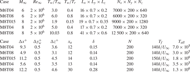
Summary of computational parameters for the DNS study. The computational domains $L_{x}, L_{y}$ and $L_{z}$ are non-dimensionalized by 1 inch (Pirozzoli et al. Reference Pirozzoli, Grasso and Gatski2004).

In this study, ${f}_{ra}$ represents the Reynolds average (spanwise and time average) of $f$, and the fluctuating counterpart of the Reynolds average is defined as ${f}'=f-{f}_{ra}$. Moreover, ${f}_{fa}={(\rho f)}_{ra}/{\rho }_{ra}$ denotes the Favre average (spanwise and time average) of $f$. The fluctuating counterpart is ${f}''=f-{f}_{fa}$.

The governing equation of kinetic energy is given by (Wang et al. Reference Wang, Wan, Chen and Chen2018, Reference Wang, Wan, Chen, Xie, Zheng, Wang and Chen2020)

(2.10)\begin{equation} \frac{\partial }{\partial t}\left( \tfrac{1}{2}\rho u_{i}^{2} \right)={-}J-\varPhi -D, \end{equation}

where $J$ is the spatial convection term, $\varPhi$ is the pressure dilatation term and $D$ is the viscous dissipation term. These terms can be written as

(2.11)$$\begin{gather} J= \frac{\partial }{\partial x_{j}}\left( \tfrac{1}{2}\rho u_{i}^{2}u_{j}+pu_{j}-\frac{u_{i}\sigma _{ij}}{Re} \right), \end{gather}$$

(2.12)$$\begin{gather}\varPhi ={-}p\frac{\partial u_{i}}{\partial x_{i}}={-}p\theta , \end{gather}$$

(2.13)$$\begin{gather}D= \frac{\sigma _{ij}}{Re}\frac{\partial u_{i}}{\partial x_{j}}=\frac{\sigma _{ij}S_{ij}}{Re}, \end{gather}$$

where $\theta$ is the velocity divergence and $S_{ij}= ( 1/2 ) ( \partial u_{i}/\partial x_{j}+\partial u_{j}/\partial x_{i} )$ is the strain-rate tensor.

The average of kinetic energy can be derived as

(2.14)\begin{equation} \frac{\partial }{\partial t} \left\langle \tfrac{1}{2}\rho u_{i}^{2} \right\rangle ={-}\langle J \rangle-\langle \varPhi \rangle -\langle D \rangle. \end{equation}

Here $\langle \,f \rangle$ represents the average of variable $f$ in streamwise, wall-normal and spanwise directions and time. Also, $\varepsilon \equiv \langle D \rangle$ is the average of viscous dissipation.

3. Dynamic equations of the filtered kinetic energy

In the following sections, the filtered method is used to investigate the effects of compressibility and wall temperature on the inter-scale transfer of kinetic energy.

The filtered field for a variable $f$ can be defined as

(3.1)\begin{equation} \bar{f}( \boldsymbol{x} )=\int d^{3}\boldsymbol{r}G_{l} ( \boldsymbol{r} )f( \boldsymbol{x}+\boldsymbol{r} ), \end{equation}

where $G_{l} ( \boldsymbol {r} )\equiv l^{-3}G ( \boldsymbol {r}/l )$ is the filter function, and $G ( \boldsymbol {r} )$ is a normalized window function. Here, $l$ is the filter width associated with the wavelength of the smallest scale retained by the filtering operation. The symbol $\tilde {f}=\bar {\rho f}/\bar {\rho }$ represents the Favre filtered field. In the present study, the top-hat filter is used, which can be calculated in one dimension by (Martin et al. Reference Martin, Piomelli, Candler and Hussaini2000; Wang et al. Reference Wang, Wan, Chen and Chen2018)

(3.2)\begin{equation} \bar{f}=\frac{1}{4n}\left( \,f_{i-n}+2\sum_{j=i-n+1}^{i+n-1}f_{j}+\,f_{i+n} \right), \end{equation}

where the filter width is $l=2n{\rm \Delta} x$. It should be noted that in order to precisely investigate the properties of the inter-scale transfer of kinetic energy along the wall-normal direction, the filtering technique is only applied on the streamwise and spanwise directions, that is, no filter is employed for the wall-normal direction.

The filtered equations for the density and momentum are (Wang et al. Reference Wang, Wan, Chen and Chen2018, Reference Wang, Wan, Chen, Xie, Zheng, Wang and Chen2020)

(3.3)$$\begin{gather} \frac{\partial \bar{\rho }}{\partial t}+\frac{\partial ( \bar{\rho }\tilde{u}_{j} )}{\partial x_{j}}=0, \end{gather}$$

(3.4)$$\begin{gather}\frac{\partial ( \bar{\rho }\tilde{u}_{i} )}{\partial t}+\frac{\partial [ \bar{\rho }\tilde{u}_{i}\tilde{u}_{j}+\bar{p}\delta _{ij} ]}{\partial x_{j}}={-}\frac{\partial ( \bar{\rho }\tilde{\tau }_{ij} )}{\partial x_{j}}+\frac{1}{Re}\frac{\partial \bar{\sigma}_{ij}}{\partial x_{j}}, \end{gather}$$

where the SGS stress is $\bar {\rho }\tilde {\tau }_{ij}=\bar {\rho } ( \widetilde {u_{i}u_{j}}-\tilde {u}_{i}\tilde {u}_{j} )$. Thus, it is straightforward to derive the filtered equation for the filtered kinetic energy $(1/2)\bar {\rho }\tilde {u}_{i}^{2}$ (Aluie Reference Aluie2011, Reference Aluie2013; Wang et al. Reference Wang, Wan, Chen and Chen2018):

(3.5)\begin{equation} \frac{\partial }{\partial t}\left( \tfrac{1}{2}\bar{\rho }\tilde{u}_{i}^{2} \right)={-}J_{l}-\varPhi _{l}-\varPi _{l}-D_{l}. \end{equation}

Here $J_{l}$ is the filtered spatial convection term, $\varPhi _{l}$ is the filtered pressure dilatation term, $\varPi _{l}$ is the SGS kinetic energy flux term and $D_{l}$ is the filtered viscous dissipation term. These terms can be written as

(3.6)$$\begin{gather} J_{l}= \frac{\partial }{\partial x_{j}}\left( \tfrac{1}{2}\bar{\rho }\tilde{u}_{i}^{2}\tilde{u}_{j}+\bar{p}\tilde{u}_{j}+\bar{\rho }\tilde{\tau }_{ij}\tilde{u}_{i}-\frac{\tilde{u}_{i}\bar{\sigma}_{ij}}{Re} \right), \end{gather}$$

(3.7)$$\begin{gather}\varPhi _{l}={-}\bar{p}\frac{\partial \tilde{u}_{i}}{\partial x_{i}}, \end{gather}$$

(3.8)$$\begin{gather}\varPi _{l}={-}\bar{\rho }\tilde{\tau }_{ij}\frac{\partial \tilde{u}_{i}}{\partial x_{j}}={-}\bar{\rho} \tilde{\tau}_{ij}\tilde{S}_{ij}, \end{gather}$$

(3.9)$$\begin{gather}D_{l}= \frac{\bar{\sigma}_{ij}}{Re}\frac{\partial \tilde{u}_{i}}{\partial x_{j}}=\frac{\bar{\sigma}_{ij} \tilde{S}_{ij}}{Re}, \end{gather}$$

where the filtered strain-rate tensor $\tilde {S}_{ij}$ is defined as $\tilde {S}_{ij}= ( 1/2 ) ( \partial \tilde {u}_{i}/\partial x_{j}+\partial \tilde {u}_{j}/\partial x_{i} )$.

To determine the properties of inter-scale transfer of kinetic energy along the wall-normal direction, the streamwise–spanwise average of the filtered kinetic energy can be written as

(3.10)\begin{equation} \frac{\partial }{\partial t}\left \langle \tfrac{1}{2}\bar{\rho }\tilde{u}_{i}^{2}\right \rangle _{xz} ={-}\langle J_{l}\rangle _{xz}-\langle \varPhi _{l} \rangle _{xz}-\langle \varPi _{l}\rangle _{xz}-\langle D_{l}\rangle _{xz}.\end{equation}

Here $\langle \,f \rangle _{xz}$ represents the average of variable $f$ in streamwise and spanwise directions and time.

4. Numerical results for kinetic energy transfer along wall-normal direction

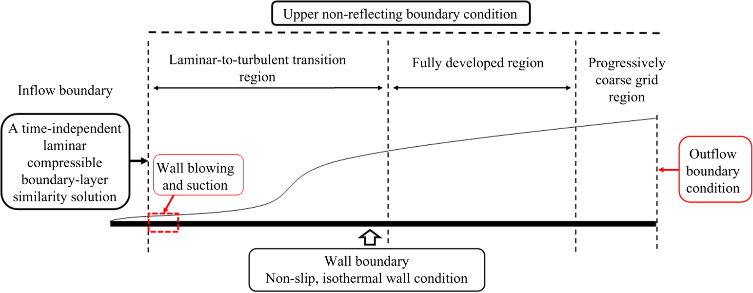
The DNS is performed using the OPENCFD code, which has been widely used and validated for compressible transitional and turbulent wall-bounded flows (Li, Fu & Ma Reference Li, Fu and Ma2008; Liang & Li Reference Liang and Li2013, Reference Liang and Li2015; Zhang et al. Reference Zhang, Bi, Hussain and She2014; She et al. Reference She, Zou, Xiao, Chen and Hussain2018; Li et al. Reference Li, Tong, Yu and Li2019; Zheng et al. Reference Zheng, Ruan, Yang, He and Chen2019). A schematic for the spatially developing turbulent boundary layer is shown in figure 1. The boundary conditions of the hypersonic turbulent boundary layer are listed as follows: inflow and outflow boundary conditions, a wall boundary condition, an upper far-field boundary condition as well as the periodic boundary condition in the spanwise direction. To be specific, a time-independent laminar compressible boundary layer similarity solution is applied at the inflow boundary. A region of wall blowing and suction (Pirozzoli et al. Reference Pirozzoli, Grasso and Gatski2004) is implemented at $4.5\leq x\leq 5$ to lead to the laminar-to-turbulent transition. Moreover, all the flow fields are extrapolated from the interior points to the outflow boundary points except the pressure in the subsonic region of the turbulent boundary layer at the outflow condition. The pressure in the subsonic region is set equal to the value of the first grid point where the flow is supersonic. In order to prevent the reflection of disturbance due to the numerical treatment of the outflow boundary condition, a progressively coarse grid is implemented in the streamwise direction near the outflow boundary condition (Pirozzoli et al. Reference Pirozzoli, Grasso and Gatski2004). Furthermore, the non-slip and isothermal conditions are applied for the wall, and the non-reflecting boundary condition is imposed for the upper boundary (Pirozzoli et al. Reference Pirozzoli, Grasso and Gatski2004). The flow initially undergoes a transition in the laminar-to-turbulent transition region, and then achieves the fully developed state in the fully developed region. Progressively coarse grid is implemented in the progressively coarse grid region in figure 1.

Figure 1.

A schematic of the computational domain.

Several hypersonic turbulent boundary layers at Mach numbers 6 and 8 with different wall temperatures are analysed numerically in the present study. The fundamental parameters of the database are listed in table 1. Here $M_{\infty }= U_{\infty }/c_{\infty }$ and $Re_{\infty }= \rho _{\infty }U_{\infty }L_{\infty }/\mu _{\infty }$ are the free-stream Mach number and Reynolds number respectively. Temperature $T_{w}$ is the wall temperature and $T_{\infty }$ is the free-stream temperature and considered to be $T_{\infty }=169.44$ K. The recovery temperature $T_{r}$ is defined as$T_{r}=T_{\infty } ( 1+r ( ( \gamma -1 )/2 )M_{\infty }^{2} )$ with recovery factor $r=0.9$ (Duan et al. Reference Duan, Beekman and Martin2010). The computational domains $L_{x}, L_{y}$ and $L_{z}$ are non-dimensionalized by $L_{\infty }=1$ inch (Pirozzoli et al. Reference Pirozzoli, Grasso and Gatski2004). Directions $x, y$ and $z$ are the streamwise, wall-normal and spanwise directions respectively; ${\rm \Delta} x^{+}={\rm \Delta} x /\delta _{\nu }$ is the normalized spacing of the streamwise direction; ${\rm \Delta} y_{w}^{+}={\rm \Delta} y_{w} /\delta _{\nu }$ is the normalized spacing of the first point off the wall; ${\rm \Delta} z^{+}={\rm \Delta} z /\delta _{\nu }$ is the normalized spacing of the spanwise direction; $\delta _{\nu }= \langle \mu _{w} \rangle _{zt}/( \langle \rho _{w} \rangle _{zt}u_{\tau })$ is the viscous length scale; $u_{\tau }=\sqrt {\tau _{w}/\rho _{w}}$ is the friction velocity; $\tau _{w}= (\mu ({\partial \langle u \rangle _{zt}}/{\partial y})) _{y=0}$ is the wall shear stress; $\rho _{w}$ is the density on the wall; and $\langle \mu _{w} \rangle _{zt}$ and $\langle \rho _{w} \rangle _{zt}$ are the spanwise and time average of viscosity and density on the wall respectively, where $\langle \,f \rangle _{zt}$ represents the spanwise and time average of variable $f$.

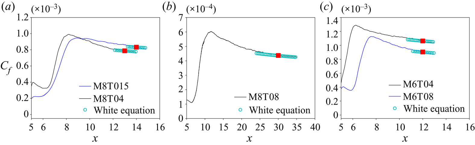
The skin-friction coefficient $c_{f}\equiv \tau _{w}/ ( \rho _{\infty }U_{\infty }^{2}/2 )$ along the streamwise direction $x$ after the region of wall blowing and suction ($x>5$) is shown in figure 2. A theoretical formula for the compressible turbulent skin friction is

(4.1)\begin{equation} C_{f}( x )=\frac{0.455}{S^{2}}\left[ \ln \left( \frac{0.06}{S}Re_{x}\frac{1}{\mu _{w}}\sqrt{\frac{1}{T_{w}}} \right) \right]^{{-}2}, \end{equation}

with $Re_{x}\equiv Re_{\infty }x$, $S=\sqrt {T_{w}-1}/\mathrm {sin}^{-1}A$ and $A= ( r_{c} ( ( \gamma -1 )/2 )Ma_{\infty }^{2} ( 1/T_{w} ) )^{1/2}$ (White Reference White2006; Zheng et al. Reference Zheng, Ruan, Yang, He and Chen2019). Equation (4.1) is represented as ‘White equation’ shown by open circles in figure 2. It is seen that the numerical simulations show a good agreement with (4.1) in the fully developed region.

Figure 2.

The skin-friction coefficient $c_{f}$ along the streamwise direction $x$ after the region of wall blowing and suction ($x>5$). The red square represents the streamwise location $x_{a}$ of the data extracted from the fully developed region of the hypersonic turbulent boundary layer. The label ‘White equation’ represents equation (4.1).

Data in a small streamwise window of $[ x_{a}-0.5\delta,x_{a}+0.5\delta ]$ extracted from the fully developed region of the hypersonic turbulent boundary layer are used for the following analysis. A number of $N$ flow-field snapshots spanning a time interval $T_{f}$ are used for analysis. The values of $x_{a}$, $\delta$, $N$ and $T_{f}$ are listed in table 1. It is noted that the red square in figure 2 represents the streamwise location $x_{a}$ of the data extracted from the hypersonic turbulent boundary layer. The streamwise location $x_{a}$ is far from the transition peak and located in the fully developed region of the hypersonic turbulent boundary layer. For the computational cost, each case takes approximately $T_{all}$ CPU hours on a 2.40 GHz Intel CPU and the values of $T_{all}$ are listed in table 1.

It should be pointed out that the present DNS database neglects the non-equilibrium and radiative effects. The reasons are as follows. The free-stream temperature is considered to be $T_{\infty }=169.44$ K. Even for the highest wall temperature case, M8T08, the greatest temperature is approximately $1700$ K, where the non-equilibrium and heat radiative effects are fairly weak in this state (Anderson Reference Anderson2006; Duan et al. Reference Duan, Beekman and Martin2011; Lagha et al. Reference Lagha, Kim, Eldredge and Zhong2011; Zhang et al. Reference Zhang, Bi, Hussain and She2014; Josyula Reference Josyula2015; She et al. Reference She, Zou, Xiao, Chen and Hussain2018) and can be neglected in the present simulation. Moreover, the greatest temperatures of cases ‘M7’, ‘M8’ and ‘M12’ in Duan et al. (Reference Duan, Beekman and Martin2011) and $M_{\infty }=7.5,10,15,20$ in Lagha et al. (Reference Lagha, Kim, Eldredge and Zhong2011) are much larger (approximately 6400 K in ‘M12’ in Duan et al. (Reference Duan, Beekman and Martin2011)) than that of the present case M8T08, and the non-equilibrium and heat radiative effects were also neglected in their study. It is worth noting that Zheng et al. (Reference Zheng, Wang, Noack, Li, Wan and Chen2020) concluded that vibrational relaxation has a negligible effect on the compression and expansion motions for both weakly and highly compressible turbulence with thermal non-equilibrium. The main purpose of this article is to investigate the effect of compressibility on the inter-scale transfer of kinetic energy. Accordingly, the neglect of non-equilibrium and heat radiative effects is a reasonable simplification for the present study of the hypersonic turbulent boundary layer.

The two-point autocorrelation coefficient $R_{\alpha \alpha }$ can be defined as

(4.2)\begin{equation} R_{\alpha \alpha }=\frac{\langle\alpha ( x,y,{z}'+z )\alpha ( x,y,{z}' ) \rangle_{zt}}{\langle\alpha ( x,y,{z}')^{2}\rangle_{zt}}. \end{equation}

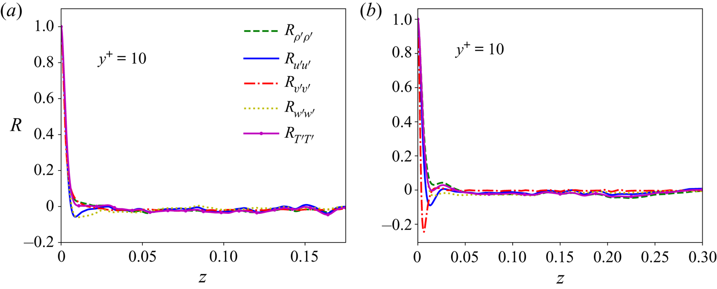
The two-point correlations of fluctuating density, velocity and temperature of M8T015 and M8T08 at $y^{+}=10$ at the streamwise location $x_{a}$ are depicted in figure 3. The $x$ axis of figure 3 represents half the size of the spanwise domain. It is shown in figure 3 that the autocorrelations drop to nearly zero at the centre of the spanwise domain, which indicates that the present computational domain in the spanwise direction is sufficiently wide. The adequacy of the computational domain size in the spanwise direction in the other three databases is also confirmed and not shown here for brevity.

Figure 3.

Distribution of the two-point correlations of fluctuating variables along the spanwise direction at $y^{+}=10$ at the streamwise location $x_{a}$ in (a) M8T015 and (b) M8T08.

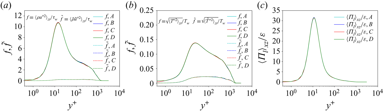
The grid resolutions of the present numerical simulations can be assessed by conducting grid convergence studies. Figure 4 shows the normalized streamwise Reynolds stress ${\langle \rho {u^{\prime \prime }}^{2} \rangle _{zt}}/{\tau _{w}}$ and the normalized filtered streamwise Reynolds stress ${\langle \bar {\rho } {{\tilde {u}}^{\prime \prime 2}} \rangle _{zt}}/{\tau _{w}}$, the normalized root-mean-square (r.m.s.) values of fluctuating temperature ${\sqrt { \langle {T^{\prime \prime }}^{2} \rangle _{zt}}}/{T_{w}}$ and the normalized r.m.s. 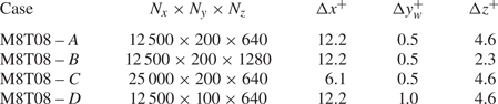values of the filtered fluctuating temperature ${\sqrt { \langle {\tilde {T}^{\prime \prime 2}} \rangle _{zt}}}/{T_{w}}$, as well as the normalized streamwise–spanwise average of the SGS flux of kinetic energy transfer at different grid resolutions listed in table 2 in M8T08. Here, the filter width is $l/\delta _{\nu }=900$. It is found that all the curves collapse indistinguishably, indicating that the grid is fine enough for the convergence of the DNS field as well as the filtered DNS field. Grid convergence of velocity and temperature fields indicates that the present grid resolution is sufficient to resolve both the turbulent and thermal boundary layers in M8T08. Moreover, grid convergence is also examined for the SGS transfer of kinetic energy as shown in figure 4(c). According to the above investigations, all the curves are coincident for different resolutions, indicating that grid resolution ‘$A$’ is sufficient to resolve the flow fields and can be used for further analysis. It is noted that the grid resolution in M8T08 is finer than that in Pirozzoli et al. (Reference Pirozzoli, Grasso and Gatski2004), where grid convergence was also checked in their study. The grid resolution in M8T08 is coarser than those in the other four cases. Moreover, the grid convergence was also checked in the other cases and the details are not shown here for brevity.

Figure 4.

Grid convergence study for M8T08. (a) The normalized streamwise Reynolds stress ${\langle \rho {u^{\prime \prime }}^{2} \rangle _{zt}}/{\tau _{w}}$ and the normalized filtered streamwise Reynolds stress ${\langle \bar {\rho } {{\tilde {u}}^{\prime \prime 2}} \rangle _{zt}}/{\tau _{w}}$ with filter width $l/\delta _{\nu }=900$. (b) The normalized r.m.s. values of fluctuating temperature ${\sqrt { \langle {T^{\prime \prime }}^{2} \rangle _{zt}}}/{T_{w}}$ and the normalized r.m.s. values of the filtered fluctuating temperature ${\sqrt { \langle {\tilde {T}^{\prime \prime 2}} \rangle _{zt}}}/{T_{w}}$ with filter width $l/\delta _{\nu }=900$. (c) The normalized streamwise–spanwise average of the SGS flux of kinetic energy transfer with filter width $l/\delta _{\nu }=900$. The symbols ‘$A$’, ‘$B$’, ‘$C$’ and ‘$D$’ represent four different grid resolutions and are listed in table 2. Grid resolution ‘$A$’ is used for further analysis.

Table 2.

Four different grid resolutions used for the grid convergence studies in M8T08.

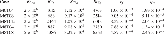
Several relevant Reynolds numbers can be defined for a compressible turbulent boundary layer. The friction Reynolds number $Re_{\tau }= \langle \rho _{w} \rangle _{zt}u_{\tau }\delta / \langle \mu _{w} \rangle _{zt}$ is defined as the ratio of the boundary layer thickness and the viscous length scale. The Reynolds number based on the momentum thickness $\theta _{th}$ and the wall viscosity, $Re_{\delta _{2}}=\rho _{\infty }u_{\infty }\theta _{th}/ \langle \mu _{w} \rangle _{zt}$, is defined as the ratio of the highest momentum to the wall shear stress. Here the momentum thickness $\theta _{th}$ is defined as

(4.3)\begin{equation} \theta _{th}=\int_{0}^{\delta }\frac{\langle \rho \rangle_{zt} \langle u\rangle_{zt}}{\rho _{\infty}u_{\infty}}\left( 1-\frac{\langle u\rangle_{zt}}{u_{\infty}} \right)\,{\textrm{d} y}, \end{equation}

where $\rho _{\infty }$ and $u_{\infty }$ are the free-stream density and streamwise velocity, and $\delta$ is the boundary layer thickness. Reynolds number $Re_{\theta _{th}}=\rho _{\infty }u_{\infty }\theta _{th}/\mu _{\infty }$ is the Reynolds number based on the momentum thickness $\theta _{th}$. Moreover, the skin-friction coefficient $c_{f}$ and wall heat flux $q_{w}\equiv (({\kappa }/{\alpha })({\partial T}/{\partial y}))|_{y=0}$ are of great importance to both practical engineering and fundamental fluid physics in a compressible turbulent boundary layer. The above global flow properties are listed in table 3.

Table 3.

Global flow properties for the DNS.

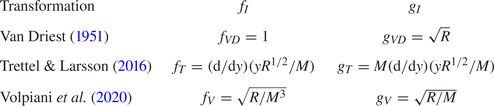
It has been shown that the Van Driest transformation (Van Driest Reference Van Driest1951) can successfully make the mean velocity profiles of adiabatic compressible wall-bounded flows consistent with those of incompressible turbulence (Duan et al. Reference Duan, Beekman and Martin2011; Pirozzoli & Bernardini Reference Pirozzoli and Bernardini2011). However, for non-adiabatic compressible wall-bounded flows, previous investigations indicate that the Van Driest transformation is no longer appropriate (Trettel & Larsson Reference Trettel and Larsson2016; Volpiani et al. Reference Volpiani, Iyer, Pirozzoli and Larsson2020). Better transformations for non-adiabatic wall turbulence have been widely investigated, which can be expressed in a general form (Modesti & Pirozzoli Reference Modesti and Pirozzoli2016) as

(4.4a,b)\begin{equation} y_{I}=\int_{0}^{y}f_{I}\,{\textrm{d} y}, \quad u_{I}=\int_{0}^{u}g_{I}\, \textrm{d} u, \end{equation}

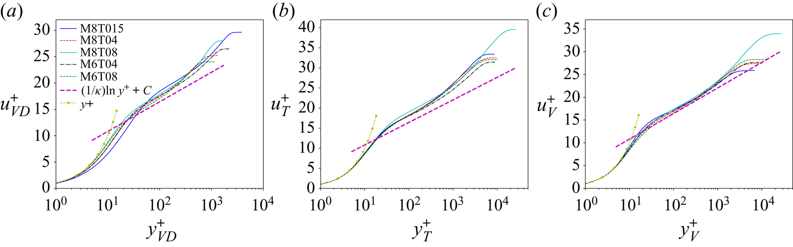
where $y_{I}$ and $u_{I}$ represent the ‘incompressible’ values obtained from different transformations. Three typical transformations are listed in table 4, namely the transformations of Van Driest (Reference Van Driest1951), Trettel & Larsson (Reference Trettel and Larsson2016) and Volpiani et al. (Reference Volpiani, Iyer, Pirozzoli and Larsson2020). Mean velocity profiles with the three transformations are shown in figure 5. It is found that the Van Driest transformation (Van Driest Reference Van Driest1951) shows the worst results, and obeys neither the linear law in the viscous sublayer nor the log law in the logarithmic region as in incompressible wall-bounded flows. This observation is consistent with previous reports in the cases with strong wall temperature gradient (Duan et al. Reference Duan, Beekman and Martin2010; Trettel & Larsson Reference Trettel and Larsson2016). The transformation of Trettel & Larsson (Reference Trettel and Larsson2016) is derived based on the mean momentum equation, and obeys the linear law in the viscous sublayer. However, a deviation from the standard log law ($u^{+}=({1}/{\kappa }) \ln y^{+}+C$) of the incompressible turbulent channel flows is observed for the transformation of Trettel & Larsson (Reference Trettel and Larsson2016). The above findings are consistent with previous observations in hypersonic turbulent boundary layers with cold wall condition (Zhang, Duan & Choudhari Reference Zhang, Duan and Choudhari2018; Volpiani et al. Reference Volpiani, Iyer, Pirozzoli and Larsson2020). The transformation of Volpiani et al. (Reference Volpiani, Iyer, Pirozzoli and Larsson2020) enforces the universality of the viscous sublayer and Morkovin-scaled shear stress, and then determines the free parameters with a data-driven method to make the mean velocity profiles of the hypersonic turbulent boundary layer consistent with the same log law as that of the incompressible wall-bounded flows. It is found that the transformation of Volpiani et al. (Reference Volpiani, Iyer, Pirozzoli and Larsson2020) gives the best results, and obeys both the linear law and log law as in incompressible wall-bounded flows.

Figure 5.

Mean velocity profiles with the transformations of (a) Van Driest (Reference Van Driest1951), (b) Trettel & Larsson (Reference Trettel and Larsson2016) and (c) Volpiani et al. (Reference Volpiani, Iyer, Pirozzoli and Larsson2020), as defined in table 4. Here $\kappa \approx 0.41$ and $C \approx 5.2$, which refer to the incompressible turbulent channel flows (Bradshaw Reference Bradshaw1977).

Table 4.

Expressions of $f_{I}$ and $g_{I}$ for various transformations in (4.4a,b), where $R= \langle \rho \rangle _{zt}/\rho _{w}$ and $M= \langle \mu \rangle _{zt}/\mu _{w}$.

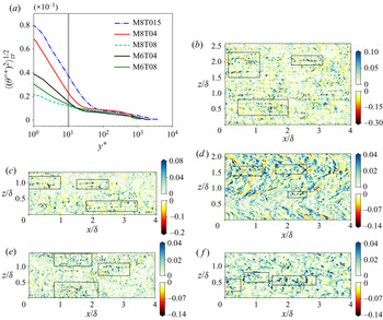
The r.m.s. values of the normalized dilatation fluctuation $\langle {({\theta }^{\prime \prime +})}^{2} \rangle _{zt}^{1/2}$ along the wall-normal direction are plotted in figure 6(a). It is found that the case with a higher Mach number and a lower wall temperature results in a much larger r.m.s. value of the normalized dilatation fluctuation $\langle {({\theta }^{\prime \prime +})}^{2} \rangle _{zt}^{1/2}$, which indicates a stronger compressibility effect in the near-wall region. Accordingly, it is observed that a colder wall temperature gives rise to a higher compressibility near the wall, which is consistent with previous observations of Duan et al. (Reference Duan, Beekman and Martin2010) and Zhang et al. (Reference Zhang, Duan and Choudhari2018). The intrinsic rationale can be explained as follows. The colder wall temperature results in a stronger temperature gradient near the wall, and the stronger temperature gradient leads to a stronger wall heat flux $q_{w}$ (listed in table 3). It is shown in table 3 that the colder wall temperature case has a larger wall heat flux $q_{w}$, which further results in a stronger compressibility effect near thewall.

Figure 6.

(a) The r.m.s. values of the normalized dilatation fluctuation $\langle {({\theta }^{\prime \prime +})}^{2} \rangle _{zt}^{1/2}$ along the wall-normal direction. Here ${\theta }''\equiv \partial {u}''_{k}/\partial x_{k}$ is the dilatation fluctuation. The grey vertical line represents the wall-normal location $y^{+}=10$. Instantaneous fields of the normalized dilatation fluctuation ${\theta }^{\prime \prime +}$ in a wall-parallel plane at $y^{+}=10$ in (b) M8T015, (c) M8T04, (d) M8T08, (e) M6T04 and (f) M6T08. Some typical alternating positive and negative patterns have been highlighted with black rectangles.

Instantaneous fields of the normalized dilatation fluctuation ${\theta }^{\prime \prime +}$ in a wall-parallel plane at $y^{+}=10$ are shown in figure 6(b–f). Specifically, negative and positive ${\theta }^{\prime \prime +}$ values form spatial spots that are well arranged as wavelike alternating patterns along the streamwise direction. The case with a higher Mach number and a lower wall temperature (particularly M8T015) exhibits much more intense alternating positive and negative structures of ${\theta }^{\prime \prime +}$, indicating a stronger compressibility. Moreover, the alternating positive and negative structures of ${\theta }^{\prime \prime +}$ are consistent with the behaviour of the dilatational velocities, which exhibit spanwise ripples travelling like streamwise wave packets from left to right shown by the instantaneous fields of the dilatational velocities in Xu et al. (Reference Xu, Wang, Wan, Yu, Li and Chen2021). The instantaneous fields of streamwise and vertical velocities as well as their solenoidal and dilatational components at $y^{+}=10$ are shown in Xu et al. (Reference Xu, Wang, Wan, Yu, Li and Chen2021).

The Lamb vector acts as a vortex force, while the Lamb vector divergence represents the dynamical mechanisms of the momentum and vorticity transport and captures the self-sustaining interactions between coherent motions in a flow field (Hamman, Klewicki & Kirby Reference Hamman, Klewicki and Kirby2008; Chen, Xu & Lu Reference Chen, Xu and Lu2010). The Lamb vector is defined as $\boldsymbol {L}\equiv \boldsymbol {\omega }\times \boldsymbol {u}$. The solenoidal and dilatational components of the Lamb vector are $\boldsymbol {L}_{s}\equiv \boldsymbol {\omega }\times \boldsymbol {u}_{s}$ and $\boldsymbol {L}_{d}\equiv \boldsymbol {\omega }\times \boldsymbol {u}_{d}$ respectively. Therefore, the Lamb vector divergence and its solenoidal and dilatational components are

(4.5)$$\begin{gather} \boldsymbol{\nabla} \boldsymbol{\cdot} \boldsymbol{L}=\boldsymbol{u}\boldsymbol{\cdot} \boldsymbol{\nabla} \times \boldsymbol{\omega }-\boldsymbol{\omega }\boldsymbol{\cdot} \boldsymbol{\omega }, \end{gather}$$

(4.6)$$\begin{gather}\boldsymbol{\nabla} \boldsymbol{\cdot} \boldsymbol{L}_{s}=\boldsymbol{u}_{s}\boldsymbol{\cdot} \boldsymbol{\nabla} \times \boldsymbol{\omega }-\boldsymbol{\omega }\boldsymbol{\cdot} \boldsymbol{\omega }, \end{gather}$$

(4.7)$$\begin{gather}\boldsymbol{\nabla} \boldsymbol{\cdot} \boldsymbol{L}_{d}=\boldsymbol{u}_{d}\boldsymbol{\cdot} \boldsymbol{\nabla} \times \boldsymbol{\omega }. \end{gather}$$

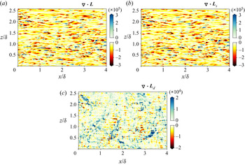
The solenoidal components are similar to the incompressible Lamb vector and Lamb vector divergence, while the dilatational components are due to the compressible effect. The instantaneous fields of the Lamb vector divergence and its solenoidal and dilatational components in a wall-parallel plane at $y^{+}=10$ in M8T015 are shown in figure 7. Based on the analysis of the Lamb vector divergence (Hamman et al. Reference Hamman, Klewicki and Kirby2008), the negative and positive values represent vorticity-bearing motions and straining motions respectively. It is shown in figure 7(a) that most of regions are occupied by the negative values of the Lamb vector divergence, indicating that the vorticity-bearing motions are dominant in the flow field. The strong positive values are always accompanied by strong negative values, indicating that the interaction between the strong straining motions and the strong vorticity-bearing motions undergoes a momentum exchange (Hamman et al. Reference Hamman, Klewicki and Kirby2008). Moreover, the instantaneous field of $\boldsymbol {\nabla } \boldsymbol {\cdot } \boldsymbol {L}_{s}$ is similar to that of $\boldsymbol {\nabla } \boldsymbol {\cdot } \boldsymbol {L}$, implying that the solenoidal component plays a dominant role in the Lamb vector divergence. The dilatational component is much smaller than the solenoidal component, and exhibits special alternating positive and negative structures, which are consistent with the behaviour of ${\theta }^{\prime \prime +}$ shown in figure 6(b–f). It is noted that the Lamb vector divergence appears as an acoustic source term in Lighthill's wave equation (Lighthill Reference Lighthill1952; Howe Reference Howe1975). Accordingly, the negative and positive structures of $\boldsymbol {\nabla } \boldsymbol {\cdot } \boldsymbol {L}_{d}$ arranged as wavelike alternating patterns are consistent with the acoustic character.

Figure 7.

The instantaneous fields of (a) the Lamb vector divergence and its (b) solenoidal and (c) dilatational components in a wall-parallel plane at $y^{+}=10$ in M8T015.

In this section, we investigate the inter-scale transfer of kinetic energy along the wall-normal direction in a hypersonic turbulent boundary layer. The effects of wall temperature as well as local compressibility on the SGS kinetic energy flux are discussed.

4.1. Statistics of kinetic energy transfer across scales along wall-normal direction

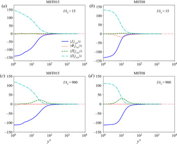
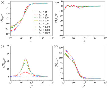
Figure 8 depicts the normalized streamwise–spanwise averages of inter-scale kinetic energy transfer terms of (3.6)–(3.9) along the wall-normal direction at filter widths $l/\delta _{\nu }=15$ and 900 in M8T015 and M8T08. It is shown that the filtered pressure dilatation term $\langle \varPhi _{l} \rangle _{xz}/\varepsilon$ is negligibly small along the wall-normal direction, while the filtered spatial convection term $\langle J _{l} \rangle _{xz}/\varepsilon$ and filtered viscous dissipation term $\langle D _{l} \rangle _{xz}/\varepsilon$ are dominant in the near-wall region and decrease rapidly away from wall. The SGS flux term $\langle \varPi _{l} \rangle _{xz}/\varepsilon$ achieves its peak value in the buffer layer at large filter width $l/\delta _{\nu }=900$.

Figure 8.

The normalized streamwise–spanwise averages of inter-scale kinetic energy transfer terms of (3.6)–(3.9) along the wall-normal direction at filter widths $l/\delta _{\nu }=15$ and 900 in M8T015 and M8T08. All the inter-scale kinetic energy transfer terms are normalized by the viscous dissipation $\varepsilon \equiv \langle D \rangle$.

The normalized streamwise–spanwise averages of inter-scale kinetic energy transfer terms of (3.6)–(3.9) along the wall-normal direction at different filter widths in M8T015 are shown in figure 9. It is shown that the normalized streamwise–spanwise averages of inter-scale kinetic energy transfer terms along the wall-normal direction are coincident for different filter widths at large scales. The behaviours of inter-scale kinetic energy transfer terms at different filter widths are qualitatively consistent with the energy-cascade hypothesis in the statistical sense: kinetic energy is generated at large scales, transferred gradually to smaller scales and finally dissipated by viscosity at small scales. The filtered viscous dissipation term $\langle D_{l} \rangle _{xz}/\varepsilon$ decays rapidly as the filter width $l/\delta _{\nu }$ increases, indicating that the kinetic energy is dissipated by viscosity at the Kolmogorov scale and is consistent with previous theoretical (Aluie Reference Aluie2011, Reference Aluie2013) and numerical (Wang et al. Reference Wang, Wan, Chen and Chen2018) analyses of the filtered viscous dissipation in isotropic compressible flows. However, the filtered viscous dissipation $\langle D_{l} \rangle _{xz}/\varepsilon$ cannot decay to zero at large scales near the wall, which will be explained later. The SGS flux $\langle \varPi _{l} \rangle _{xz}/\varepsilon$ increases from zero as the filter width $l/\delta _{\nu }$ increases from the Kolmogorov scale to the inertial range. Moreover, the average values of the SGS flux $\langle \varPi _{l} \rangle _{xz}/\varepsilon$ along the wall-normal direction at large filter widths are coincident for different filter widths, which implies the nearly statistically invariant property of kinetic energy transfer across scales in the inertial range. Accordingly, the inertial range is nearly $l/\delta _{\nu }=900\text {--}1350$. It is also worth noting that the filtered spatial convection term $\langle J_{l} \rangle _{xz}/\varepsilon$ is dominant in the near-wall region even at the largest filter width $l/\delta _{\nu }=1350$. Moreover, the filtered pressure dilatation $\langle \varPhi _{l} \rangle /\varepsilon$ decays to almost zero quickly in the buffer layer as the scale $l/\delta _{\nu }$ increases, indicating that the net contribution of pressure dilatation to the average kinetic energy is negligibly small at large scales. Similar observations have also been reported for previous studies of isotropic compressible turbulence (Aluie et al. Reference Aluie, Li and Li2012; Wang et al. Reference Wang, Shi, Wang, Xiao, He and Chen2012a, Reference Wang, Wan, Chen and Chen2018; Jagannathan & Donzis Reference Jagannathan and Donzis2016).

Figure 9.

The normalized streamwise–spanwise averages of inter-scale kinetic energy transfer terms of (3.6)–(3.9) along the wall-normal direction at different filter widths in M8T015.

It has been noted that the filtered viscous dissipation $\langle D_{l} \rangle _{xz}/\varepsilon$ cannot decay to zero at large scales near the wall. The values of $\langle D_{l} \rangle _{xz}/\varepsilon$ along with different filter widths at $y^{+}=10$, 20, 50 and 100 in M8T015 are shown in figure 10(a). It is found that $\langle D_{l} \rangle _{xz}/\varepsilon$ cannot decay to zero at large scales in the near-wall region, while at the far-wall region ($y^{+}=100$), $\langle D_{l} \rangle _{xz}/\varepsilon$ decays to almost zero in the inertial range, which is the same as the results for compressible isotropic turbulence (Wang et al. Reference Wang, Wan, Chen and Chen2018).

Figure 10.

(a) The values of $\langle D_{l} \rangle _{xz}/\varepsilon$ along with different filter widths at $y^{+}=10$, 20, 50 and 100 in M8T015. The normalized streamwise–spanwise averages of $J_{l,m}$, $J_{l,f}$, $D_{l,m}$ and $D_{l,f}$ along the wall-normal direction at filter widths (b) $l/\delta _{\nu }=15$ and (c) 900 in M8T015. The vertical dash-dotted lines from left to right represent position $y^{+}=10$, 20, 50 and 100, respectively.

The above observations can be explained as follows. A simple decomposition is applied to identify the influence of the mean flow velocities $( u_{i} )_{fa}$ (Favre average of velocities $u_{i}$), which is expressed as follows:

(4.8)$$\begin{gather} J_{l}=J_{l,m}+J_{l,f}, \end{gather}$$

(4.9)$$\begin{gather}D_{l}=D_{l,m}+D_{l,f}, \end{gather}$$

where $J_{l,m}$ and $D_{l,m}$ are the filtered spatial convection term and filtered viscous dissipation term based on the mean flow velocities $( u_{i} )_{fa}$, while $J_{l,f}$ and $D_{l,f}$ are the filtered spatial convection term and filtered viscous dissipation term resulting from the interaction between mean flow velocities $( u_{i} )_{fa}$ and fluctuating velocities ${u}_{i}''$, as well as the interaction among the fluctuating velocities ${u}_{i}''$. These terms can be written as

(4.10)$$\begin{gather} J_{l,m}=\frac{\partial }{\partial x_{j}}\left( \frac{1}{2}\bar{\rho }\widetilde{(u_{i} )_{fa}}^{2}\widetilde{(u_{j} )_{fa}}+\bar{p}\widetilde{(u_{j})_{fa}}+\bar{\rho}\widetilde{(\tau _{ij})_{fa}} \widetilde{(u_{i})_{fa}}-\frac{\widetilde{(u_{i})_{fa}} \overline{(\sigma _{ij} )_{ra}}}{Re} \right), \end{gather}$$

(4.11)$$\begin{gather}J_{l,f}=J_{l}-J_{l,m}, \end{gather}$$

(4.12)$$\begin{gather}D_{l,m}= \frac{\overline{(\sigma _{ij} )_{ra}}}{Re}\frac{\partial \widetilde{(u_{i} )_{fa}}}{\partial x_{j}}=\frac{\overline{(\sigma _{ij} )_{ra}}\widetilde{(S_{ij} )_{fa}}}{Re}, \end{gather}$$

(4.13)$$\begin{gather}D_{l,f}=D_{l}-D_{l,m}. \end{gather}$$

Here $(\sigma _{ij} )_{ra}$ is the Reynolds average of viscous stress $\sigma _{ij}$, $\widetilde { (\tau _{ij} )_{fa}}$ and $(S_{ij} )_{fa}$ are the mean SGS stress and the mean strain-rate tensor calculated by the mean velocities $( u_{i} )_{fa}$, which are defined as

(4.14)$$\begin{gather} \widetilde{(\tau _{ij} )_{fa}}=\widetilde{(u_{i} )_{fa}(u_{j} )_{fa}}-\widetilde{(u_{i} )_{fa}}\widetilde{(u_{j} )_{fa}}, \end{gather}$$

(4.15)$$\begin{gather}(S_{ij} )_{fa}=\frac{1}{2}\left( \frac{\partial (u_{i} )_{fa}}{\partial x_{j}}+\frac{\partial (u_{j} )_{fa}}{\partial x_{i}} \right). \end{gather}$$

The normalized streamwise–spanwise averages of $J_{l,m}$, $J_{l,f}$, $D_{l,m}$ and $D_{l,f}$ along the wall-normal direction at filter widths $l/\delta _{\nu }=15$ and 900 in M8T015 are depicted in figures 10(b) and 10(c). It is found that at small filter width $l/\delta _{\nu }=15, \langle D_{l,m} \rangle _{xz}/\varepsilon$ and $\langle D_{l,f} \rangle _{xz}/\varepsilon$ exhibit their peak values near the wall and drop quickly away from the wall. Moreover, $\langle D_{l,f} \rangle _{xz}/\varepsilon \ll \langle D_{l,m} \rangle _{xz}/\varepsilon$. As the filter width increases to the inertial range ($l/\delta _{\nu }=900$), $\langle D_{l,f} \rangle _{xz}/\varepsilon$ decays to almost zero along the wall-normal direction, while $\langle D_{l,m} \rangle _{xz}/\varepsilon$ is nearly unchanged along the wall-normal direction. Accordingly, the non-zero $\langle D_{l} \rangle _{xz}/\varepsilon$ in the near-wall region at large filter width is mainly due to the mean filtered viscous dissipation term $\langle D_{l,m} \rangle _{xz}/\varepsilon$. At the far-wall region (such as $y^{+}=100$ in figure 10a), $\langle D_{l,m} \rangle _{xz}/\varepsilon$ decays to almost zero, which results in the negligibly small $\langle D_{l} \rangle _{xz}/\varepsilon$ at large scales.

It is shown that $\langle J_{l,m} \rangle _{xz}/\varepsilon$ achieves its peak value near the wall, which results in the domination of the filtered spatial convection term $\langle J_{l } \rangle _{xz}/\varepsilon$ in the near-wall region; $\langle J_{l,f} \rangle _{xz}/\varepsilon$ attains its peak value in the buffer layer. As filter width increases, $\langle J_{l,m} \rangle _{xz}/\varepsilon$ is nearly unchanged along the wall-normal direction, while the magnitude of $\langle J_{l,f} \rangle _{xz}/\varepsilon$ decreases near the wall, and increases in the buffer layer.

An interesting phenomenon is found that the wall temperature has a significant influence on the kinetic energy transfer, especially on the filtered pressure dilatation term $\varPhi _{l}$ and the SGS flux term $\varPi _{l}$. The normalized streamwise–spanwise average of the filtered pressure dilatation $\langle \varPhi _{l} \rangle _{xz}/\varepsilon$ and the r.m.s. values of the filtered pressure dilatation $\varPhi _{l,rms}/\varepsilon$ along the wall-normal direction at filter widths $l/\delta _{\nu }=15$, 300 and 900 in M8T015 and M8T08 are shown in figure 11. The r.m.s. value of the filtered pressure dilatation $\varPhi _{l,rms}$ is defined as $\varPhi _{l,rms}=\sqrt { \langle ( \varPhi _{l} )^{2} \rangle _{xz}}$. It is shown that $\langle \varPhi _{l} \rangle _{xz}/\varepsilon$ and $\varPhi _{l,rms}/\varepsilon$ decrease quickly as filter width increases, indicating that the net contribution of pressure dilatation to the average kinetic energy is prominent only at small scales, and the pressure dilatation has a significant effect on the local conversion between kinetic energy and internal energy. The fact that $\varPhi _{l,rms}/\varepsilon \gg \langle \varPhi _{l} \rangle _{xz}/\varepsilon$ indicates the significant cancellation between positive and negative values of filtered pressure dilatation. Moreover, $\varPhi _{l,rms}/\varepsilon$ attains its peak value near the wall, and is much larger in M8T015 than in M8T08, which indicates that the cold wall temperature induces a much stronger compressibility in the near-wall region.

Figure 11.

The normalized streamwise–spanwise average of the filtered pressure dilatation $\langle \varPhi _{l} \rangle _{xz}/\varepsilon$ and the r.m.s. values of the filtered pressure dilatation $\varPhi _{l,rms}/\varepsilon$ along the wall-normal direction at filter widths $l/\delta _{\nu }=15$, 300 and 900 in (a) M8T015 and (b) M8T08.

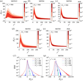
The probability density function (PDF) of the normalized SGS flux $\varPi _{l} /\varepsilon$ along the wall-normal direction in the inertial range $l/\delta _{\nu }=900$ is shown in figure 12(a–e). It is found that the negative values of the normalized SGS flux $\varPi _{l} /\varepsilon$ appear in some flow regions as indicated by the negative side of the PDF, especially in M8T015. The negative value of SGS flux can be interpreted as the SGS backscatter of kinetic energy, i.e. the reverse transfer of kinetic energy from small scales to large scales. The PDF of the SGS flux exhibits a strong positive skewness in the inertial range, especially in M6T04, M6T08, M8T04 and M8T08, where almost all values of the SGS flux are larger than zero. It is also found that the degree of the positive skewness becomes weaker as the wall temperature decreases, indicating that the cold wall temperature enhances the local reverse transfer of kinetic energy from small scales to large scales. The above observation indicates that the kinetic energy transfer has a tendency to be from large scales to small scales, and the cold wall temperature suppresses this local direct transfer of kinetic energy. The PDF of the normalized SGS flux $\varPi _{l} /\varepsilon$ at $y^{+}=10$ at different filter widths in M8T015 and M8T08 is depicted in figure 12(f,g). It is illustrated that local reverse transfer of kinetic energy appears frequently at small scales. As filter width increases, local reverse transfer of kinetic energy is markedly suppressed. It is also found that the peak values of the PDF of the SGS flux increase as filter width increases, indicating that more positive SGS flux appears at large scales. The two tails of the PDF of the SGS flux become longer as filter width decreases, due to the fact that local energy transfer is more intermittent at small scales than at large scales. The differences of PDFs in M8T015 and M8T08 are more significant at small scales than at large scales, implying that the effect of wall temperature is more prominent at small scales.

Figure 12.

The PDF of the normalized SGS flux $\varPi _{l} /\varepsilon$ along the wall-normal direction in the inertial range $l/\delta _{\nu }=900$ in (a) M8T015, (b) M8T04, (c) M8T08, (d) M6T04 and (e) M6T08. The PDF of the normalized SGS flux $\varPi _{l} /\varepsilon$ at $y^{+}=10$ at different filter widths in (f) M8T015 and (g) M8T08.

4.2. Effect of fluctuating velocity divergence on SGS flux of kinetic energy

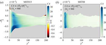
The filtered fluctuating velocity divergence is denoted by ${\theta }''_{l}={\partial \tilde {u}_{i}^{''}}/{\partial x_{i}}$, representing the strength of local compression and expansion motions. Figure 13 shows the conditional streamwise–spanwise average of normalized SGS flux $\langle \varPi _{l}/\varepsilon \mid {{\theta }^{\prime \prime }_{l}}^{+} \rangle _{xz}$ along the wall-normal direction in the inertial range $l/\delta _{\nu }=900$ in M8T015 and M8T08. It is found that $\langle \varPi _{l}/\varepsilon \mid {{\theta }^{\prime \prime }_{l}}^{+} \rangle _{xz}$ is positive almost everywhere, except for some strong expansion regions in M8T015, indicating that the direct transfer of kinetic energy from large scales to small scales is dominant in the hypersonic turbulent boundary layer. It is also found that $\langle \varPi _{l}/\varepsilon \mid {{\theta }^{\prime \prime }_{l}}^{+} \rangle _{xz}$ decreases as the normalized filtered fluctuating velocity divergence ${\theta ^{\prime \prime }_{l}}^{+}$ increases from negative to positive, indicating that the local reverse transfer of kinetic energy is mainly concentrated in the expansion region. Wall temperature has a significant effect on $\langle \varPi _{l}/\varepsilon \mid {{\theta }^{\prime \prime }_{l}}^{+} \rangle _{xz}$. It is shown that negative values of $\langle \varPi _{l}/\varepsilon \mid {{\theta }^{\prime \prime }_{l}}^{+} \rangle _{xz}$ appear in some strong expansion regions in M8T015, and the values of $\langle \varPi _{l}/\varepsilon \mid {{\theta }^{\prime \prime }_{l}}^{+} \rangle _{xz}$ in M8T015 are smaller than those in M8T08, indicating that the cold wall temperature enhances the reverse transfer of kinetic energy.

Figure 13.

The streamwise–spanwise average of the normalized SGS flux $\varPi _{l}/\varepsilon$ conditioned on the normalized filtered fluctuating velocity divergence ${\theta ^{\prime \prime }_{l}}^{+}$ along the wall-normal direction at filter width $l/\delta _{\nu }=900$ in (a) M8T015 and (b) M8T08.

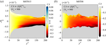
A variable $\beta _{l}$ is introduced to investigate the relation between the filtered strain-rate tensor and the SGS stress, which is defined as (Wang et al. Reference Wang, Wan, Chen and Chen2018)

(4.16)\begin{equation} \beta _{l}=\frac{\tilde{\tau }_{ij}\tilde{S}_{ij}}{| \tilde{\tau } || \tilde{S} |}, \end{equation}

where $| \tilde {\tau } |=\sqrt {\tilde {\tau }_{ij}\tilde {\tau }_{ij}}$ and $| \tilde {S} |=\sqrt {\tilde {S}_{ij}\tilde {S}_{ij}}$. Figure 14 shows the streamwise–spanwise average of $\beta _{l}$ conditioned on the normalized filtered fluctuating velocity divergence ${\theta ^{\prime \prime }_{l}}^{+}$ along the wall-normal direction at filter width $l/\delta _{\nu }=900$ in M8T015 and M8T08. A negative $\langle \beta _{l}\mid {{\theta }^{\prime \prime }_{l}}^{+} \rangle _{xz}$ represents the direct transfer of kinetic energy from large scales to small scales, while a positive $\langle \beta _{l}\mid {{\theta }^{\prime \prime }_{l}}^{+} \rangle _{xz}$ represents the reverse transfer of kinetic energy from small scales to large scales (Wang et al. Reference Wang, Wan, Chen and Chen2018). It is shown that $\langle \beta _{l}\mid {{\theta }^{\prime \prime }_{l}}^{+} \rangle _{xz}$ is almost zero near the wall, implying the nearly perpendicular relation between the filtered strain-rate tensor and the SGS stress in the near-wall region. As wall-normal distance increases, the magnitudes of $\langle \beta _{l}\mid {{\theta }^{\prime \prime }_{l}}^{+} \rangle _{xz}$ increase, demonstrating the high efficiency of inter-scale kinetic energy transfer far from the wall. Accordingly, the wall suppresses the efficiency of the inter-scale kinetic energy transfer. Moreover, $\langle \beta _{l}\mid {{\theta }^{\prime \prime }_{l}}^{+} \rangle _{xz}$ exhibits more negative values in strong compression regions, demonstrating the higher efficiency of direct inter-scale kinetic energy transfer induced by compression motions. The magnitude of $\langle \beta _{l}\mid {{\theta }^{\prime \prime }_{l}}^{+} \rangle _{xz}$ is smaller in M8T015 than in M8T08, indicating that the cold wall temperature weakens the efficiency of the inter-scale kinetic energy transfer.

Figure 14.

The streamwise–spanwise average of $\beta _{l}$ conditioned on the normalized filtered fluctuating velocity divergence ${\theta ^{\prime \prime }_{l}}^{+}$ along the wall-normal direction at filter width $l/\delta _{\nu }=900$ in (a) M8T015 and (b) M8T08.

5. Mean-fluctuating decomposition and Helmholtz decomposition on SGS flux of kinetic energy

In this section, mean-fluctuating decomposition is applied to identify the influence of mean flow velocities. Moreover, Helmholtz decomposition of the velocity fields is also introduced to explore the compressibility effect in an isothermal hypersonic turbulent boundary layer.

The velocity field can be divided into $\boldsymbol {u}= (\boldsymbol {u})_{fa}+{\boldsymbol {u}}''$. Furthermore, the fluctuating velocities ${\boldsymbol {u}}''$ can be decomposed into a solenoidal (${\boldsymbol {u}}''_{s}$) and a dilatational (${\boldsymbol {u}}''_{d}$) component.

Accordingly, the SGS stress $\bar {\rho }\tilde {\tau }_{ij}$ can be divided into

(5.1)\begin{equation} \bar{\rho }\tilde{\tau }_{ij}=\tilde{\tau }_{m,ij}+\tilde{\tau }_{f,ij}+\tilde{\tau }_{in,ij}, \end{equation}

where $\tilde {\tau }_{m,ij}$ is the mean SGS stress term based on the mean velocities $(\boldsymbol {u})_{fa}, \tilde {\tau }_{f,ij}$ is the fluctuating SGS stress resulting from the fluctuating velocities ${\boldsymbol {u}}''$ and $\tilde {\tau }_{in,ij}$ is the SGS stress due to the interaction between the mean velocities $(\boldsymbol {u})_{fa}$ and fluctuating velocities ${\boldsymbol {u}}''$. These terms can be written as

(5.2)$$\begin{gather} \tilde{\tau }_{m,ij}\equiv\bar{\rho }(\widetilde{(u_{i} )_{fa}(u_{j} )_{fa}}-\widetilde{(u_{i} )_{fa}}\widetilde{(u_{j} )_{fa}} ), \end{gather}$$

(5.3)$$\begin{gather}\tilde{\tau }_{f,ij}\equiv\bar{\rho }(\widetilde{{u}''_{i} {u}''_{j} }-\widetilde{{u}}''_{i}\widetilde{{u}}''_{j} ), \end{gather}$$

(5.4)$$\begin{gather}\tilde{\tau }_{in,ij}\equiv \bar{\rho }\tilde{\tau }_{ij}-\tilde{\tau }_{m,ij}-\tilde{\tau }_{f,ij}. \end{gather}$$

Therefore, the SGS flux of kinetic energy $\varPi _{l}$ can be decomposed by

(5.5)\begin{align} \varPi _{l} &={-}\tilde{\tau }_{m,ij}\widetilde{( S_{ij} )_{fa}}-\tilde{\tau }_{m,ij}\widetilde{ {S}}''_{ij}-\tilde{\tau }_{f,ij}\widetilde{( S_{ij} )_{fa}}\nonumber\\ &\quad -\tilde{\tau }_{f,ij}\widetilde{ {S}}''_{ij}-\tilde{\tau }_{in,ij}\widetilde{( S_{ij} )_{fa}}-\tilde{\tau }_{in,ij}\widetilde{ {S}}''_{ij}\nonumber\\ &\equiv \varPi _{mm,l}+\varPi _{mf,l}+\varPi _{fm,l}+\varPi _{ff,l}+\varPi _{inm,l}+\varPi _{inf,l}. \end{align}

Here ${S}''_{ij}$ is the strain-rate tensor in terms of the fluctuating velocities ${\boldsymbol {u}}''$, which is defined as ${S}''_{ij}=(\partial {u}''_{i}/\partial x_{j}+\partial {u}''_{j}/\partial x_{i})/2$.

On the basis of Helmholtz decomposition, $\tilde {\tau }_{f,ij}$ and ${S}''_{ij}$ can be further decomposed into

(5.6)\begin{equation} \tilde{\tau }_{f,ij}=\tilde{\tau }_{fs,ij}+\tilde{\tau }_{fd,ij}+\tilde{\tau }_{fsd,ij}, {S}''_{ij}={S}''_{s,ij}+{S}''_{d,ij}, \end{equation}

where

(5.7)$$\begin{gather} \tilde{\tau }_{fs,ij}\equiv\bar{\rho }(\widetilde{{u}''_{s,i} {u}''_{s,j} }-\widetilde{{u}}''_{s,i}\widetilde{{u}}''_{s,j}), \end{gather}$$

(5.8)$$\begin{gather}\tilde{\tau }_{fd,ij}\equiv\bar{\rho }(\widetilde{{u}''_{d,i} {u}''_{d,j} }-\widetilde{{u}}''_{d,i}\widetilde{{u}}''_{d,j}), \end{gather}$$

(5.9)$$\begin{gather}\tilde{\tau }_{fsd,ij}\equiv\tilde{\tau }_{f,ij}-\tilde{\tau }_{fs,ij}-\tilde{\tau }_{fd,ij}, \end{gather}$$

(5.10)$$\begin{gather}{S}''_{s,ij}\equiv (\partial {u}''_{s,i}/\partial x_{j}+\partial {u}''_{s,j}/\partial x_{i})/2, \end{gather}$$

(5.11)$$\begin{gather}{S}''_{d,ij}\equiv (\partial {u}''_{d,i}/\partial x_{j}+\partial {u}''_{d,j}/\partial x_{i})/2. \end{gather}$$

Thus, two dominant components $\varPi _{fm,l} \equiv -\tilde {\tau }_{f,ij}\widetilde { ( S_{ij} )_{fa}}$ and $\varPi _{ff,l} \equiv -\tilde {\tau }_{f,ij}\widetilde { {S}}''_{ij}$ of the SGS flux of kinetic energy $\varPi _{l}$ can be decomposed by

(5.12)\begin{align} \varPi _{fm,l}&={-}\tilde{\tau }_{fs,ij}\widetilde{( S_{ij} )_{fa}}-\tilde{\tau }_{fd,ij}\widetilde{( S_{ij} )_{fa}}-\tilde{\tau }_{fsd,ij}\widetilde{( S_{ij} )_{fa}}\nonumber\\ &\equiv \varPi _{fsm,l}+\varPi _{fdm,l}+\varPi _{fsdm,l}, \end{align}

(5.13)\begin{align} \varPi _{ff,l}&={-}\tilde{\tau }_{fs,ij}\widetilde{{S}}''_{s,ij}-\tilde{\tau }_{fs,ij}\widetilde{{S}}''_{d,ij}-\tilde{\tau }_{fd,ij}\widetilde{{S}}''_{s,ij} \nonumber\\ &\quad -\tilde{\tau }_{fd,ij}\widetilde{{S}}''_{d,ij}-\tilde{\tau }_{fsd,ij}\widetilde{{S}}''_{s,ij}-\tilde{\tau }_{fsd,ij}\widetilde{{S}}''_{d,ij}\nonumber\\ &\equiv \varPi _{fsfs,l}+\varPi _{fsfd,l}+\varPi _{fdfs,l}+\varPi _{fdfd,l}+\varPi _{fsdfs,l}+\varPi _{fsdfd,l}. \end{align}

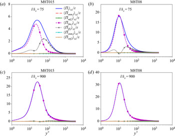
The normalized streamwise–spanwise averages of the SGS flux of kinetic energy $\varPi _{l}$ and its decomposed components in (5.5) along the wall-normal direction at filter widths $l/\delta _{\nu }=75$ and 900 in M8T015 and M8T08 are depicted in figure 15. It is shown that at small scales $l/\delta _{\nu }=75$, the component $\langle \varPi _{fm,l} \rangle _{xz}$ dominates in $\langle \varPi _{l} \rangle _{xz}$ and the component $\langle \varPi _{ff,l} \rangle _{xz}$ also plays a significant role in $\langle \varPi _{l} \rangle _{xz}$, while other components are negligible. Accordingly, $\langle \varPi _{l} \rangle _{xz}$ is mainly determined by the interaction between the fluctuating SGS stress $\tilde {\tau }_{f,ij}$ and the filtered strain-rate tensor $\widetilde { S}_{ij}$ at small scales. However, as the inertial range increases to $l/\delta _{\nu }=900, \langle \varPi _{l} \rangle _{xz}$ is mainly dominated by the component $\langle \varPi _{fm,l} \rangle _{xz}$. The component $\langle \varPi _{ff,l} \rangle _{xz}$ is relatively small and other components are negligible. Thus, $\langle \varPi _{l} \rangle _{xz}$ is mainly dominated by the interaction between the fluctuating SGS stress $\tilde {\tau }_{f,ij}$ and the mean filtered strain-rate tensor $\widetilde { ( S_{ij} )_{fa}}$ in the inertial range. Moreover, $\langle \varPi _{fm,l} \rangle _{xz}$ attains its peak value in the buffer layer. The value of $\langle \varPi _{fm,l} \rangle _{xz}$ is positive, indicating that the interaction between the fluctuating SGS stress $\tilde {\tau }_{f,ij}$ and the mean filtered strain-rate tensor $\widetilde { ( S_{ij} )_{fa}}$ mainly leads to the direct transfer of kinetic energy from large scales to small scales. Moreover, it is shown that the magnitude of $\langle \varPi _{ff,l} \rangle _{xz}$ decreases as filter width increases, indicating that the positive and negative values of $\varPi _{ff,l}$ are largely cancelled in the inertial range.

Figure 15.

The normalized streamwise–spanwise averages of the SGS flux of kinetic energy $\varPi _{l}$ and its decomposed components in (5.5) along the wall-normal direction at filter widths $l/\delta _{\nu }=75$ and $900$ in M8T015 and M8T08.

According to the above observations, only $\varPi _{fm,l} /\varepsilon$ and $\varPi _{ff,l} /\varepsilon$ play significant roles in $\varPi _{l} /\varepsilon$. Therefore, we focus on $\varPi _{fm,l} /\varepsilon$ and $\varPi _{ff,l} /\varepsilon$ in further discussion.

The normalized streamwise–spanwise averages of $\varPi _{fm,l}$ and its decomposed components in (5.12) along the wall-normal direction at filter width $l/\delta _{\nu }=900$ in M8T015 and M8T08 are shown in figure 16(a,b). It is found that $\langle \varPi _{fm,l} \rangle _{xz}$ is mainly dominated by its solenoidal component $\langle \varPi _{fsm,l} \rangle _{xz}$. Here $\langle \varPi _{fsm,l} \rangle _{xz}$ achieves its peak value in the buffer layer, indicating a strong intensity of fluctuating solenoidal kinetic energy transfer in this region. In the inertial range $l/\delta _{\nu }=900, \langle \varPi _{fsm,l} \rangle _{xz}$ is even larger than $\langle \varPi _{fm,l} \rangle _{xz}$, and $\langle \varPi _{fsdm,l} \rangle _{xz}$ counteracts the contribution of the solenoidal component $\langle \varPi _{fsm,l} \rangle _{xz}$. The component $\langle \varPi _{fsdm,l} \rangle _{xz}$ achieves its peak value in the buffer layer, and its peak location is similar to that of $\langle \varPi _{fsm,l} \rangle _{xz}$. The dilatational component $\langle \varPi _{fdm,l} \rangle _{xz}$ is larger in M8T015 than in M8T08, indicating that the cold wall temperature enhances the compressibility effect. Also, $\langle \varPi _{fm,l} \rangle _{xz}$ in M8T015 is mainly dominated by the dilatational component $\langle \varPi _{fdm,l} \rangle _{xz}$ near the wall, while the solenoidal component $\langle \varPi _{fsm,l} \rangle _{xz}$ plays a predominant role far from the wall, implying that the cold wall temperature enhances the compressibility mainly in the near-wall region. Both $\langle \varPi _{fsm,l} \rangle _{xz}$ and $\langle \varPi _{fdm,l} \rangle _{xz}$ are positive, while $\langle \varPi _{fsdm,l} \rangle _{xz}$ is negative, indicating that the interaction between the fluctuating solenoidal SGS stress $\tilde {\tau }_{fs,ij}$ and the mean filtered strain-rate tensor $\widetilde { ( S_{ij} )_{fa}}$ as well as the interaction between the fluctuating dilatational SGS stress $\tilde {\tau }_{fd,ij}$ and the mean filtered strain-rate tensor $\widetilde { ( S_{ij} )_{fa}}$ mainly lead to the direct transfer of kinetic energy, while the interaction between $\tilde {\tau }_{fsd,ij}$ and $\widetilde { ( S_{ij} )_{fa}}$ mainly leads to the reverse transfer of kinetic energy.

Figure 16.

The normalized streamwise–spanwise averages of $\varPi _{fm,l}$ and its decomposed components in (5.12) along the wall-normal direction at filter widths $l/\delta _{\nu }=900$ in (a) M8T015 and (b) M8T08. (c) The normalized streamwise–spanwise averages of $\varPi _{ff,l}$ and its decomposed components in (5.13) along the wall-normal direction at filter width $l/\delta _{\nu }=900$ in M8T015.

The normalized streamwise–spanwise averages of $\varPi _{ff,l}$ and its decomposed components in (5.13) along the wall-normal direction at filter width $l/\delta _{\nu }=900$ in M8T015 are shown in figure 16(c). It is found that the solenoidal component $\langle \varPi _{fsfs,l} \rangle _{xz}$ dominates in $\langle \varPi _{ff,l} \rangle _{xz}$. Other components have small contributions to $\langle \varPi _{ff,l} \rangle _{xz}$. In the inertial range $l/\delta _{\nu }=900$, a strong local reverse fluctuating solenoidal kinetic energy transfer appears in the buffer layer.

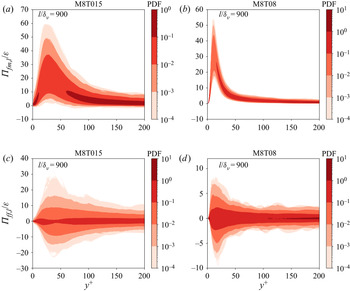
The PDFs of the components $\varPi _{fm,l} /\varepsilon$ and $\varPi _{ff,l} /\varepsilon$ along the wall-normal direction in the inertial range $l/\delta _{\nu }=900$ in M8T015 and M8T08 are shown in figure 17. The PDF of the component $\varPi _{fm,l} /\varepsilon$ is similar to that of $\varPi _{l} /\varepsilon$, and exhibits a strong positive skewness. Negative values of $\varPi _{fm,l} /\varepsilon$ only appear in M8T015, implying that the cold wall temperature enhances the local reverse kinetic energy transfer due to the interaction between the fluctuating SGS stress $\tilde {\tau }_{f,ij}$ and the mean filtered strain-rate tensor $\widetilde { ( S_{ij} )_{fa}}$. However, the PDF of $\varPi _{ff,l} /\varepsilon$ is slightly positively skewed and totally different from the PDFs of $\varPi _{fm,l} /\varepsilon$ and $\varPi _{l} /\varepsilon$, where strong intensities of negative values of $\varPi _{ff,l} /\varepsilon$ appear in both M8T015 and M8T08.

Figure 17.

The PDFs of the components $\varPi _{fm,l} /\varepsilon$ and $\varPi _{ff,l} /\varepsilon$ along the wall-normal direction in the inertial range $l/\delta _{\nu }=900$ in M8T015 and M8T08.

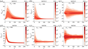
The PDFs of the components $\varPi _{fsm,l} /\varepsilon$, $\varPi _{fdm,l} /\varepsilon$ and $\varPi _{fsfs,l} /\varepsilon$ along the wall-normal direction in the inertial range $l/\delta _{\nu }=900$ in M8T015 and M8T08 are shown in figure 18. The PDF of the component $\varPi _{fsm,l} /\varepsilon$ is similar to that of $\varPi _{fm,l} /\varepsilon$, and exhibits a strong positive skewness. Negative values of $\varPi _{fsm,l} /\varepsilon$ only exist in M8T015, implying that the cold wall temperature enhances the local reverse kinetic energy transfer due to the interaction between the fluctuating solenoidal SGS stress $\tilde {\tau }_{fs,ij}$ and the mean filtered strain-rate tensor $\widetilde { ( S_{ij} )_{fa}}$. Moreover, $\varPi _{fdm,l} /\varepsilon$ is positively skewed. The widest PDF of $\varPi _{fdm,l} /\varepsilon$ appears near the wall, indicating that the local transfer of fluctuating dilatational kinetic energy is concentrated in the near-wall region. The PDF of $\varPi _{fsfs,l} /\varepsilon$ is similar to that of $\varPi _{ff,l} /\varepsilon$. It is seen that $\varPi _{fsfs,l} /\varepsilon$ is slightly positively skewed, and strong intensities of negative values of $\varPi _{fsfs,l} /\varepsilon$ appear in the buffer layer, indicating the strong local reverse transfer of fluctuating solenoidal kinetic energy in this region.

Figure 18.

The PDFs of the components $\varPi _{fsm,l} /\varepsilon$, $\varPi _{fdm,l} /\varepsilon$ and $\varPi _{fsfs,l} /\varepsilon$ along the wall-normal direction in the inertial range $l/\delta _{\nu }=900$ in M8T015 and M8T08.

Figures 19(a) and 19(b) show the conditional streamwise–spanwise average $\langle \varPi _{fm,l}/\varepsilon \mid {{\theta }^{\prime \prime }_{l}}^{+} \rangle _{xz}$ and $\langle \varPi _{ff,l}/\varepsilon \mid {{\theta }^{\prime \prime }_{l}}^{+} \rangle _{xz}$ along the wall-normal direction in the inertial range $l/\delta _{\nu }=900$ in M8T015. The value of $\langle \varPi _{fm,l}/\varepsilon \mid {{\theta }^{\prime \prime }_{l}}^{+} \rangle _{xz}$ is positive and increases as the magnitude of ${{\theta }^{\prime \prime }_{l}}^{+}$ increases, indicating that strong direct transfer caused by $\varPi _{fm,l}$ mainly appears in strong expansion and compression regions. Figure 19(c) shows the conditional streamwise–spanwise average $\langle \varPi _{ff,l}/\varepsilon \mid {{\theta }^{\prime \prime }_{l}}^{+} \rangle _{xz}$ at $y^{+}=20$ for different filter widths $l/\delta _{\nu }=750$, 900, 1050 and 1200 in M8T015. It is found that the conditional average $\langle \varPi _{ff,l}/\varepsilon \mid {{\theta }^{\prime \prime }_{l}}^{+} \rangle _{xz}$ is nearly independent of filter width $l/\delta _{\nu }$, especially in the weak compression and expansion regions at filter widths $l/\delta _{\nu }=900$, 1050 and 1200 in the inertial range, which is similar to previous observations for compressible isotropic turbulence (Wang et al. Reference Wang, Wan, Chen and Chen2018). However, in strong compression and expansion regions where the magnitude of the normalized fluctuating velocity divergence ${\theta ^{\prime \prime }_{l}}^{+}$ is large, the values of $\langle \varPi _{ff,l}/\varepsilon \mid {{\theta }^{\prime \prime }_{l}}^{+} \rangle _{xz}$ are quite scattered mainly due to the lack of samples. The observation of the scale-invariant property of the conditional average $\langle \varPi _{ff,l}/\varepsilon \mid {{\theta }^{\prime \prime }_{l}}^{+} \rangle _{xz}$ is consistent with the well-known energy cascade hypothesis (Meneveau & Katz Reference Meneveau and Katz2000; Pope Reference Pope2000). In the inertial range, the inter-scale transfer of kinetic energy as well as the conditional average of normalized SGS flux are nearly scale-invariant. It is shown that positive values of $\langle \varPi _{ff,l}/\varepsilon \mid {{\theta }^{\prime \prime }_{l}}^{+} \rangle _{xz}$ often appear in compression regions, while negative values of $\langle \varPi _{ff,l}/\varepsilon \mid {{\theta }^{\prime \prime }_{l}}^{+} \rangle _{xz}$ often exist in expansion regions, which implies that compression motions have a major contribution to the direct transfer of fluctuating kinetic energy, while expansion motions play a significant role in the reverse transfer of fluctuating kinetic energy. This observation is consistent with the phenomenon in compressible isotropic turbulence (Wang et al. Reference Wang, Wan, Chen and Chen2018).

Figure 19.

The streamwise–spanwise average of the component (a) $\varPi _{fm,l}/\varepsilon$ and (b) $\varPi _{ff,l}/\varepsilon$ conditioned on the normalized filtered fluctuating velocity divergence ${\theta ^{\prime \prime }_{l}}^{+}$ along the wall-normal direction at filter width $l/\delta _{\nu }=900$ in M8T015. (c) The streamwise–spanwise average of the component $\varPi _{ff,l}/\varepsilon$ conditioned on the normalized filtered fluctuating velocity divergence ${\theta ^{\prime \prime }_{l}}^{+}$ at $y^{+}=20$ for different filter widths $l/\delta _{\nu }=750$, 900, 1050 and 1200 in M8T015.

6. Summary and conclusion

In this paper, the filtering method is applied to investigate the kinetic energy transfer in a hypersonic turbulent boundary layer for different Mach numbers and wall temperature ratios. The effects of compressibility and wall temperature on the kinetic energy transfer and the SGS flux of kinetic energy are systematically discussed. Among three typical transformations of mean velocity profiles, the transformation of Volpiani et al. (Reference Volpiani, Iyer, Pirozzoli and Larsson2020) exhibits the best results, and obeys both the same linear law and log law as in incompressible wall-bounded flows. A colder wall temperature with a stronger wall temperature gradient results in a stronger wall heat flux, which further gives rise to a stronger compressibility effect near the wall.

The streamwise–spanwise average values of inter-scale kinetic energy transfer terms are discussed. The average filtered spatial convection term $\langle J _{l} \rangle _{xz}/\varepsilon$ and average filtered viscous dissipation term $\langle D _{l} \rangle _{xz}/\varepsilon$ are dominant in the near-wall region, and decrease rapidly away from wall. However, the average filtered pressure dilatation term $\langle \varPhi _{l} \rangle _{xz}/\varepsilon$ is negligibly small along the wall-normal direction at large scales, indicating that the net contribution of pressure dilatation to the average kinetic energy is negligibly small at large scales. The average SGS flux of kinetic energy $\langle \varPi _{l} \rangle _{xz}/\varepsilon$ increases from zero as the filter width $l/\delta _{\nu }$ increases from the Kolmogorov scale to the inertial range, and achieves its peak value in the buffer layer. The behaviours of inter-scale kinetic energy transfer terms are consistent with the kinetic energy cascade scenario.

The PDF of the normalized SGS flux $\varPi _{l}/\varepsilon$ exhibits a strong positive skewness. It is found that a cold wall temperature enhances the local reverse transfer of kinetic energy from small scales to large scales, and suppresses the local direct transfer of kinetic energy from large scales to small scales. It is also shown that the effect of wall temperature is more prominent at small scales.

The effect of local compressibility is further examined by the conditional average of normalized SGS flux with respect to the filtered velocity divergence. It is found that the direct transfer of kinetic energy is dominant in the hypersonic turbulent boundary layer, and the local reverse transfer of kinetic energy is mainly concentrated in the expansion region. Moreover, the wall, especially with cold wall temperature, can suppress the efficiency of inter-scale kinetic energy transfer.

Mean-fluctuating decomposition and Helmholtz decomposition on SGS flux of kinetic energy are introduced. The streamwise–spanwise average of the SGS flux of kinetic energy $\langle \varPi _{l} \rangle _{xz}$ is mainly determined by the interaction between the fluctuating SGS stress $\tilde {\tau }_{f,ij}$ and the filtered strain-rate tensor $\widetilde { S_{ij} }$ at small scales, while only $\langle \varPi _{fm,l} \rangle _{xz}$ is dominant in $\langle \varPi _{l} \rangle _{xz}$ in the inertial range. The value of $\langle \varPi _{fm,l} \rangle _{xz}$ is positive along the wall-normal direction and mainly dominated by its solenoidal component $\langle \varPi _{fsm,l} \rangle _{xz}$. A strong transfer of the solenoidal component of fluctuating kinetic energy due to $\varPi _{fsm,l}$ is identified in the buffer layer, while a significant transfer of the dilatational component of fluctuating kinetic energy due to $\varPi _{fdm,l}$ is observed in the near-wall region. In the inertial range, $\langle \varPi _{ff,l} \rangle _{xz}$ is dominated by its solenoidal component $\langle \varPi _{fsfs,l} \rangle _{xz}$, and exhibits a negative peak value in the buffer layer, indicating a strong local reverse transfer of fluctuating kinetic energy in this region. Conditional streamwise–spanwise average $\langle \varPi _{ff,l}/\varepsilon \mid {{\theta }^{\prime \prime }_{l}}^{+} \rangle _{xz}$ illustrates that compression motions have a major contribution to the direct transfer of fluctuating kinetic energy, while expansion motions play a significant role in the reverse transfer of fluctuating kinetic energy.

In conclusion, the various effects of the wall temperature and compressibility on the SGS flux of kinetic energy in a hypersonic turbulent boundary layer are revealed. The cold wall temperature significantly enhances the compressibility in the near-wall region and a local reverse SGS flux of kinetic energy in the strong expansion region, which should be considered in the LES modelling of hypersonic turbulent boundary layers.