1. INTRODUCTION
Airy wave packets were originally introduced as a solution of the Schrodinger equation for a particle in free fall (Berry & Balazs, Reference Berry and Balazs1979). Although it was demonstrated that the Airy wave packet can remain a uniform profile and transverse acceleration during propagation in free space, the Airy wave packet is not square integrable and it contains an infinite energy. Experimentally, optical Airy beams can be generated by introducing a finite-energy Airy beam (Siviloglou & Christodoulides, Reference Siviloglou and Christodoulides2007; Siviloglou et al., Reference Siviloglou, Brokly, Dogariu and Christodoulides2007). Recently, the study of Airy beam has attracted immense attention due to its fascinating behaviors such as limited-diffraction, transverse acceleration, and self-healing, as well as their potential applications in optics (Bandres & Gutierrez-Vega, Reference Bandres and Gutierrez-Vega2007; Broky et al., Reference Broky, Siviloglou, Dogariu and Christodoulides2008). Many works have been performed to investigate both theoretically and experimentally the underlying physics and the application of the Airy beam. Kasparian and Wolf (Reference Kasparian and Wolf2009) elaborated that the transverse complex energy fluxes of the Airy beam cause the beam to curve when it propagates. Based on the characteristic intensity pattern and the parabolic curve propagation of the beam, a new feature in optical micromanipulation was reported using the Airy beam that drags particles into the main intensity maximum of the beam and guides the particles vertically along the trajectory. This interesting property of Airy beam leads to the removal of particles and cells from a section of a sample chamber (Baumgartl et al., Reference Baumgartl, Mazilu and Dholakia2008). The evanescent waves of nonparaxial Airy beams (Novitsky & Novitsky, Reference Novitsky and Novitsky2009), the form of the Poynting vector, linear and angular momenta of an Airy beam (Sztul & Alfano, Reference Sztul and Alfano2008), and nonlinear generation and manipulation of the Airy beam (Ellenbogen et al., Reference Ellenbogen, Voloch-Bloch, Ganany-Padowicz and Arie2009), have also been demonstrated. The effect of Kerr nonlinearity on an Airy beam has been recently elaborated (Chen et al., Reference Chen, Yin, Chu and Wang2010). The evolution characteristics of an Airy beam in nonlinear medium including the laser filamentation (Polynkin et al., Reference Polynkin, Kolesik and Moloney2009a), curved plasma channel generation (Polynkin et al. Reference Polynkin, Kolesik, Moloney, Siviloglou and Christodoulides2009b), supercontinuum (Ament et al., Reference Ament, Polynkin and Moloney2011), and solitary wave generation (Kaminer et al., Reference Kaminer, Segev and Christodoulides2011) have been examined. The experimental realization of a plasmonic Airy beam on a silver surface (Li et al., Reference Li, Li, Wang, Zhang and Zhu2011) and the generation and the near-field imaging of nondiffracting plasmonic Airy beams (Minovich et al., Reference Minovich, Klein, Janunts, Pertsch, Neshev and Kivshar2011) have been reported. The Wigner distribution function was used to study the Airy beam by Chen et al. (Reference Chen, Zheng and Dai2011) to analyze these novel properties of an Airy beam. The results showed that these novel properties of an Airy beam are attributed to the continuum of sideways contributions to the field. The phenomenon was also analyzed using the method of geometrical optics and the Kirchhoff-Huygens integral to explain the novel features of Airy beam by Kaganovsky and Heyman (Reference Kaganovsky and Heyman2010).
Vortices have been the subject of many studies and appear in many branches of physics (Pismen, Reference Pismen1999; Mellado et al., Reference Mellado, Hacyan and Jauregui2006; Desai & Pant, Reference Desai and Pant2000). Optical vortices have been applied in a variety of fields due to its intriguing properties such as stimulated emission depletion microscopy, particle manipulation, and laser processing. Recently, Mazilu et al. (Reference Mazilu, Baumgartl, Cizmar and Dholakia2009) reported the accelerating vortices embedded in Airy beams by employing a spiral phase on a cubic phase pattern. Dai et al. (Reference Dai, Liu, Luo and Sun2010; Reference Dai, Liu, Luo and Sun2011) studied the propagation dynamics of Airy beams carrying an optical vortex that can be generated by a phase spatial light modulator. More recently, Chen and Ooi (Reference Chen and Ooi2011) studied the Wigner distribution function of a vortex Airy beam. Their analytical study indicates that the destructive interference of certain classical waves resembles the nonclassical lights such as those due to quantum effects.
Another interesting feature of vortex Airy beam is its vector structure. Recently, the vector structure of electromagnetic waves with different spatial distribution have attracted the interest of many researchers (Luo & Lü, Reference Luo and Lü2010; Guo et al., Reference Guo, Chen and Zhuang2006; Zhou, Reference Zhou2006). Any arbitrary polarized electromagnetic beam can be decomposed into transverse electric mode (TE) term and transverse electric magnetic mode (TM) term in term of its vector angular spectrum (Mart'ınez-Herrero et al., Reference Mart'ınez-Herrero, Mejas, Bosch and Carnicer2001; Zhou et al., Reference Zhou, Ni and Zhang2007; Wu et al., Reference Wu, Lou and Zhou2008). The vector angular spectrum method is also an effective method to derive exact solutions of Maxwell's equations. In this work, we studied the vector structure of vortex Airy beams analytically in the far-field. The analytical vectorial structure of vortex Airy beams in the far-field is obtained using the vector angular spectrum and the method of stationary phase. An analytical expression of the TE and TM terms for the nth-order vortex Airy beam is computed in Section 2. The numerical results of energy flux distributions of vortex Airy beams in far-field are analyzed. In Section 3, the effects of different modulation parameters on the energy flux distributions of vortex Airy beam and its TE and TM terms in far-field are discussed.
2. ANALYTICAL VECTORIAL STRUCTURE
In the Cartesian coordinate system, the z-axis is taken to be the propagation axis. The field function of an nth-order vortex centered at (x d, y d) in the initial finite energy Airy beam, which is polarized in the x-direction, can be expressed as (Mazilu et al., Reference Mazilu, Baumgartl, Cizmar and Dholakia2009; Dai et al., Reference Dai, Liu, Luo and Sun2010; Reference Dai, Liu, Luo and Sun2011)
 $$\eqalign{& \left({\matrix{ {E_x \lpar x\comma \; y\semicolon \; z=0\rpar } \cr {E_y \lpar x\comma \; y\semicolon \; z=0\rpar } \cr } } \right) \cr & \quad = \left({\matrix{ {Ai\lpar s_x \rpar \exp \lpar as_x \rpar Ai\lpar s_y \rpar \exp \lpar as_y \rpar [ \lpar x - x_d \rpar + i \lpar y - y_d \rpar ] ^n } \cr 0 } } \right)\comma \;}$$
where A 0 is the amplitude of the complex amplitude E(x,y,z = 0). s x = x/x 0, and s y = y/y 0 represent the dimensionless transverse coordinates. x 0 and y 0 are arbitrary transverse scales. a is a positive parameter to ensure the containment of the infinite Airy tail. The time dependent factor exp(−iωt) is omitted in Eq. (1), and ω is the circular frequency. The transverse components of the vector angular spectrum A x(u,v) and A y(u,v) are given by the Fourier transform of the initial field as (Mart'ınez-Herrero et al., Reference Mart'ınez-Herrero, Mejas, Bosch and Carnicer2001; Guo et al., Reference Guo, Chen and Zhuang2006; Zhou, Reference Zhou2006)
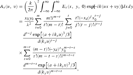 $$\eqalign{A_x \lpar u\comma \; v \rpar &= \mathop{\left({\displaystyle{k \over {2{\rm \pi} }}} \right)}\nolimits^2 \int_{ - \infty }^\infty \, \int_{ - \infty }^\infty \, E_x \lpar x\comma \; y\comma \; 0\rpar \exp[ \!\!- ik\lpar ux+vy\rpar ] dxdy \cr & =\displaystyle{{x_0 y_0 } \over {{\rm \lambda} ^2 }}\sum\limits_{t=0}^m \, \displaystyle{{m!i^{m - t} } \over {t!\lpar m - t\rpar !}}\sum\limits_{\,j=0}^t \, \displaystyle{{t!\lpar \!- x_d \rpar ^j x_0^{t - j} } \over {\,j!\lpar t - j\rpar !i^{t - j} }} \cr & \quad\displaystyle{{d^{t - j} \exp\left[{\lpar a+ik_x u\rpar ^3 /3} \right]} \over {d\lpar k_x u\rpar ^{t - j} }} \cr & \times \sum\limits_{s=0}^{m - t} \, \displaystyle{{\lpar m - t\rpar !\lpar \!\!- y_d \rpar ^s y_0^{m - t - s} } \over {s!\lpar m - t - s\rpar !i^{m - t - s} }} \cr & \quad\displaystyle{{d^{m - t - s} \exp\left[{\lpar a+ik_y v\rpar ^3 /3} \right]} \over {d\lpar k_y v\rpar ^{m - t - s} }}\comma \;}$$
 $$A_y \lpar u\comma \; v\rpar =0\comma \;$$
where k x = kx 0 , k y = ky 0, and k denotes wavenumber. u, v, and m represent the directional cosines of x,y, and z-components of the transverse wave vector, respectively. The propagating electromagnetic field of a vortex Airy beam can be decomposed accordingly into the TE and TM terms as
 $$E\lpar r\rpar =E_{TE} \lpar r\rpar +E_{TM} \lpar r\rpar \comma \;$$
 $$H\lpar r\rpar =H_{TE} \lpar r\rpar +H_{TM} \lpar r\rpar \comma \;$$
where the TE and TM terms of the propagating electromagnetic field for a vortex Airy beam can be written in the following forms (Luo & Lü, Reference Luo and Lü2010; Guo et al., Reference Guo, Chen and Zhuang2006; Zhou, Reference Zhou2006):
 $$\eqalign{E_{TE} \lpar r\rpar & =\int_{ - \infty }^\infty \, \int_{ - \infty }^\infty \, \displaystyle{v \over {u^2+v^2 }}\left({ve_x - ue_y } \right)A_x \lpar u\comma \; v\rpar \cr & \quad \exp\left[{ik\lpar ux+vy+mz\rpar } \right]dudv\comma \; }$$
 $$\eqalign{E_{TM} \lpar r\rpar & =\int_{ - \infty }^\infty \, \int_{ - \infty }^\infty \, \displaystyle{u \over {\lpar u^2+v^2 \rpar m}}\left[{ume_x+vme_y - \lpar u^2+v^2 \rpar e_z } \right]\cr & \quad A_x \lpar u\comma \; v\rpar \exp\left[{ik\lpar ux+vy+mz\rpar } \right]dudv\comma \; }$$
 $$\eqalign{H_{TE} \lpar r\rpar & =\sqrt {\displaystyle{{{\rm \varepsilon} _0 } \over {{\rm \mu} _0 }}} \int_{ - \infty }^\infty \, \int_{ - \infty }^\infty \, \displaystyle{v \over {\lpar u^2+v^2 \rpar }}\left[{ume_x+vme_y - \lpar u^2+v^2 \rpar e_z } \right]\cr & \quad A_x \lpar u\comma \; v\rpar \exp\left[{ik\lpar ux+vy+mz\rpar } \right]dudv\comma \; }$$
 $$\eqalign{H_{TM} \lpar r\rpar & =- \sqrt {\displaystyle{{{\rm \varepsilon} _0 } \over {{\rm \mu} _0 }}} \int_{ - \infty }^\infty \, \int_{ - \infty }^\infty \, \displaystyle{u \over {\lpar u^2+v^2 \rpar m}}\left({ve_x - ue_y } \right)\cr & \quad A_x \lpar u\comma \; v\rpar \exp\left[{ik\lpar ux+vy+mz\rpar } \right]dudv\comma \; }$$
where e x, e y, and e z are the unit vectors in x, y, and z-direction, respectively. According to the stationary-phase approach (Zhou, Reference Zhou2006; Stamnes, Reference Stamnes1983; Mandel, & Wolf, Reference Mandel and Wolf1995), the double integrals of Eq. (6) have an asymptotic value as kr → ∞ (Stamnes, Reference Stamnes1983; Mandel, & Wolf, Reference Mandel and Wolf1995)
 $$\eqalign{E_{TE} & =\displaystyle{{i{\rm \lambda} } \over r}\sum\limits_{{\rm \alpha}=1}^w \, \displaystyle{{{\rm \sigma} _{\rm \alpha} } \over {\lpar {\rm \mu} _{\rm \alpha} {\rm \nu} _{\rm \alpha} - {\rm \gamma} _{\rm \alpha} ^2 \rpar ^{1/2} }}F\lpar u_{\rm \alpha}\comma \; v_{\rm \alpha} \rpar \cr & \quad \exp [ ikrG\lpar u_{\rm \alpha}\comma \; v_{\rm \alpha}\comma \; x\comma \; y\rpar ] \comma \; }$$
where w is the number of stationary points, and
 $$F\lpar u_{\rm \alpha}\comma \; v_{\rm \alpha} \rpar =\displaystyle{{v_{\rm \alpha} } \over {u_{\rm \alpha} ^2+v_{\rm \alpha} ^2 }}\left({v_{\rm \alpha} e_x - u_{\rm \alpha} e_y } \right)A_x \lpar u_{\rm \alpha}\comma \; v_{\rm \alpha} \rpar \comma \;$$
and
 $$G\lpar u_{\rm \alpha}\comma \; v_{\rm \alpha}\comma \; x\comma \; y\rpar =\left[{u_{\rm \alpha} x+v_{\rm \alpha} y+\lpar 1 - u_{\rm \alpha} ^2 - v_{\rm \alpha} ^2 \rpar ^{1/2} z} \right]/r.$$
The stationary points (u α, v α) are solutions of the equations
 $$\displaystyle{{\partial G\lpar u_{\rm \alpha}\comma \; v_{\rm \alpha}\comma \; x\comma \; y\rpar } \over {\partial u_{\rm \alpha} }}=\displaystyle{1 \over r}\left({x - \displaystyle{{zu_{\rm \alpha} } \over {\lpar 1 - u_{\rm \alpha} ^2 - v_{\rm \alpha} ^2 \rpar ^{1/2} }}} \right)=0\comma \;$$
 $$\displaystyle{{\partial G\lpar u_{\rm \alpha}\comma \; v_{\rm \alpha}\comma \; x\comma \; y\rpar } \over {\partial v_{\rm \alpha} }}=\displaystyle{1 \over r}\left({y - \displaystyle{{zv_{\rm \alpha} } \over {\lpar 1 - u_{\rm \alpha} ^2 - v_{\rm \alpha} ^2 \rpar ^{1/2} }}} \right)=0.$$
The solutions can be obtained by solving Eqs. (13) and (14),
 $$u_1=x/r\comma \; v_1=y/r.$$
There is only one stationary point, which means w = 1. The parameters μ1, ν1 , γ1, and σ1 thus can be obtained by
 $${\rm \mu} _1=\displaystyle{{\partial ^2 G\lpar u_1\comma \; v_1\comma \; x\comma \; y\rpar } \over {\partial u_1^2 }}=- \left({1+\displaystyle{{x^2 } \over {z^2 }}} \right)\comma \;$$
 $${\rm \nu} _1=\displaystyle{{\partial ^2 G\lpar u_1\comma \; v_1\comma \; x\comma \; y\rpar } \over {\partial v_1^2 }}=- \left({1+\displaystyle{{y^2 } \over {z^2 }}} \right)\comma \;$$
 $${\rm \gamma} _1=\displaystyle{{\partial ^2 F\lpar u_1\comma \; v_1\comma \; x\comma \; y\rpar } \over {\partial u_1 \partial v_1 }}=- \displaystyle{{xy} \over {z^2 }}\comma \;$$
 $${\rm \sigma} _1=- 1.$$
Substituting Eqs. (15)–(19) into Eq. (10), the analytical electric field of the TE term in the far-field is found to be
 $$\eqalign{ E_{TE} \lpar r\rpar &=- \displaystyle{{ix_0 y_0 yz} \over {r^2 {\rm \lambda} \lpar x^2+y^2 \rpar }}\left({ye_x - xe_y } \right)\cr & \quad \times \sum\limits_{t=0}^m \, \displaystyle{{m!i^{m - t} } \over {t!\lpar m - t\rpar !}}\sum\limits_{\,j=0}^t \, \displaystyle{{t!\lpar \!\!- x_d \rpar ^j x_0^{t - j} } \over {\,j!\lpar t - j\rpar !i^{t - j} }}\cr & \quad \displaystyle{{d^{t - j} \exp\left[{\lpar a+ik_x x/r\rpar ^3 /3} \right]} \over {d\lpar k_x x/r\rpar ^{t - j} }} \cr & \quad \times \sum\limits_{s=0}^{m - t} \, \displaystyle{{\lpar m - t\rpar !\lpar \!\!- y_d \rpar ^s y_0^{m - t - s} } \over {s!\lpar m - t - s\rpar !i^{m - t - s} }}\cr & \quad \displaystyle{{d^{m - t - s} \exp\left[{\lpar a+ik_y y/r\rpar ^3 /3} \right]} \over {d\lpar k_y y/r\rpar ^{m - t - s} }}\exp\lpar ikr\rpar .}$$
The corresponding magnetic field of the TE term is
 $$\eqalign{ H_{TE} \lpar r\rpar &=- \displaystyle{{ix_0 y_0 yz} \over {r^3 {\rm \lambda} \lpar x^2+y^2 \rpar }}\sqrt {\displaystyle{{{\rm \varepsilon} _0 } \over {{\rm \mu} _0 }}} \left[{xze_x+yze_y - \lpar x^2+y^2 \rpar e_z } \right]\cr & \quad \times \sum\limits_{t=0}^m \, \displaystyle{{m!i^{m - t} } \over {t!\lpar m - t\rpar !}}\sum\limits_{\,j=0}^t \, \displaystyle{{t!\lpar \!\!- x_d \rpar ^j x_0^{t - j} } \over {\,j!\lpar t - j\rpar !i^{t - j} }}\cr & \quad \displaystyle{{d^{t - j} \exp\left[{\lpar a+ik_x x/r\rpar ^3 /3} \right]} \over {d\lpar k_x x/r\rpar ^{t - j} }} \cr & \quad \times \sum\limits_{s=0}^{m - t} \, \displaystyle{{\lpar m - t\rpar !\lpar \!\!- y_d \rpar ^s y_0^{m - t - s} } \over {s!\lpar m - t - s\rpar !i^{m - t - s} }}\cr & \quad \displaystyle{{d^{m - t - s} \exp\left[{\lpar a+ik_y y/r\rpar ^3 /3} \right]} \over {d\lpar k_y y/r\rpar ^{m - t - s} }}\exp\lpar ikr\rpar \comma \; }$$
Similarly, the analytical TM term can be obtained as
 $$\eqalign{ E_{TM} \lpar r\rpar& =- \displaystyle{{ix_0 y_0 x} \over {r^2 {\rm \lambda} \lpar x^2+y^2 \rpar }}\left[{xze_x+yze_y - \lpar x^2+y^2 \rpar e_z } \right]\cr & \quad \times \sum\limits_{t=0}^m \, \displaystyle{{m!i^{m - t} } \over {t!\lpar m - t\rpar !}}\sum\limits_{\,j=0}^t \, \displaystyle{{t!\lpar \!\!- x_d \rpar ^j x_0^{t - j} } \over {\,j!\lpar t - j\rpar !i^{t - j} }}\displaystyle{{d^{t - j} \exp\left[{\lpar a+ik_x x/r\rpar ^3 /3} \right]} \over {d\lpar k_x x/r\rpar ^{t - j} }} \cr & \quad \times \sum\limits_{s=0}^{m - t} \, \displaystyle{{\lpar m - t\rpar !\lpar \!\!- y_d \rpar ^s y_0^{m - t - s} } \over {s!\lpar m - t - s\rpar !i^{m - t - s} }}\cr & \quad \displaystyle{{d^{m - t - s} \exp\left[{\lpar a+ik_y y/r\rpar ^3 /3} \right]} \over {d\lpar k_y y/r\rpar ^{m - t - s} }}\exp\lpar ikr\rpar \comma \; }$$
 $$\eqalign{ H_{TM} \lpar r\rpar &=\displaystyle{{ix_0 y_0 x} \over {r{\rm \lambda} \lpar x^2+y^2 \rpar }}\sqrt {\displaystyle{{{\rm \varepsilon} _0 } \over {{\rm \mu} _0 }}} \left({ye_x - xe_y } \right)\cr & \quad \times \sum\limits_{t=0}^m \, \displaystyle{{m!i^{m - t} } \over {t!\lpar m - t\rpar !}}\sum\limits_{\,j=0}^t \, \displaystyle{{t!\lpar \!\!- x_d \rpar ^j x_0^{t - j} } \over {\,j!\lpar t - j\rpar !i^{t - j} }}\displaystyle{{d^{t - j} \exp\left[{\lpar a+ik_x x/r\rpar ^3 /3} \right]} \over {d\lpar k_x x/r\rpar ^{t - j} }} \cr & \quad \times \sum\limits_{s=0}^{m - t} \, \displaystyle{{\lpar m - t\rpar !\lpar \!\!- y_d \rpar ^s y_0^{m - t - s} } \over {s!\lpar m - t - s\rpar !i^{m - t - s} }}\cr & \quad \displaystyle{{d^{m - t - s} \exp\left[{\lpar a+ik_y y/r\rpar ^3 /3} \right]} \over {d\lpar k_y y/r\rpar ^{m - t - s} }}\exp\lpar ikr\rpar .}$$
The analytical TE and TM terms of the n = first-order vortex Airy mode in the far-field can be expressed as
 $$E_{TE} \lpar r\rpar =- \displaystyle{{ix_0 y_0 yz} \over {r^2 {\rm \lambda} \lpar x^2+y^2 \rpar }}\left({ye_x - xe_y } \right){\rm \beta}\comma \;$$
 $$H_{TE} \lpar r\rpar =- \displaystyle{{ix_0 y_0 yz} \over {r^3 {\rm \lambda} \lpar x^2+y^2 \rpar }}\sqrt {\displaystyle{{{\rm \varepsilon} _0 } \over {{\rm \mu} _0 }}} \left[{xze_x+yze_y - \lpar x^2+y^2 \rpar e_z } \right]{\rm \beta}\comma \;$$
 $$E_{TM} \lpar r\rpar =- \displaystyle{{ix_0 y_0 x} \over {r^2 {\rm \lambda} \lpar x^2+y^2 \rpar }}\left[{xze_x+yze_y - \lpar x^2+y^2 \rpar e_z } \right]{\rm \beta}\comma \;$$
 $$H_{TM} \lpar r\rpar =\displaystyle{{ix_0 y_0 x} \over {r{\rm \lambda} \lpar x^2+y^2 \rpar }}\sqrt {\displaystyle{{{\rm \varepsilon} _0 } \over {{\rm \mu} _0 }}} \left({ye_x - xe_y } \right){\rm \beta}\comma \;$$
with
 $$\eqalign{{\rm \beta} &=\left[{ix_0 \lpar a+ik_x x/r\rpar ^2 - y_0 \lpar a+ik_y y/r\rpar ^2 - x_d - iy_d } \right]\cr &\quad \times \exp\left[{\lpar a+ik_x x/r\rpar ^3 /3+\lpar a+ik_y y/r\rpar ^3 /3+ikr} \right].}$$
For the n = 2nd-order vortex Airy mode, the TE and TM terms in the far-field are
 $$E_{TE} \lpar r\rpar =- \displaystyle{{ix_0 y_0 yz} \over {r^2 {\rm \lambda} \lpar x^2+y^2 \rpar }}\left({ye_x - xe_y } \right)\Gamma\comma \;$$
 $$H_{TE} \lpar r\rpar =- \displaystyle{{ix_0 y_0 yz} \over {r^3 {\rm \lambda} \lpar x^2+y^2 \rpar }}\sqrt {\displaystyle{{{\rm \varepsilon} _0 } \over {{\rm \mu} _0 }}} \left[{xze_x+yze_y - \lpar x^2+y^2 \rpar e_z } \right]\Gamma\comma \;$$
 $$E_{TM} \lpar r\rpar =- \displaystyle{{ix_0 y_0 x} \over {r^2 {\rm \lambda} \lpar x^2+y^2 \rpar }}\left[{xze_x+yze_y - \lpar x^2+y^2 \rpar e_z } \right]\Gamma\comma \;$$
 $$H_{TM} \lpar r\rpar =\displaystyle{{ix_0 y_0 x} \over {r{\rm \lambda} \lpar x^2+y^2 \rpar }}\sqrt {\displaystyle{{{\rm \varepsilon} _0 } \over {{\rm \mu} _0 }}} \left({ye_x - xe_y } \right)\Gamma\comma \;$$
with
 $$\eqalign{& \Gamma = \exp[ \lpar a+ik_x x/r\rpar ^3 /3+\lpar a+ik_y y/r\rpar ^3 /3+ikr ] \cr & \quad \times \Big[\!\! - \lpar a+ik_x x/r \rpar \lpar 2+\lpar a+ik_x x/r \rpar ^3 \rpar x_0^2+\lpar x_d+iy_d \rpar ^2 \cr & \quad - 2i\lpar a+ik_x x/r \rpar ^2 \lpar a+ik_y y/r \rpar ^2 x_0 y_0 \cr &\quad +\lpar a+ik_x x/r \rpar \lpar 2+\lpar a+ik_y y/r \rpar ^3 \rpar y_0^2 \cr & \quad - 2ix_0 \lpar a+ik_x x/r \rpar ^2 \lpar x_d+iy_d \rpar \cr & \quad - 2y_0\lpar a+ik_y y/r \rpar ^2 \lpar ix_d+y_d \rpar \Big] .}$$
3. ENERGY FLUX DISTRIBUTIONS IN THE FAR-FIELD
We can now analyze the energy flux distributions of the vortex Airy beam in far-field by the z component of the time-average Poynting vector, as follows:
 $$\left\langle {S_z } \right\rangle=\displaystyle{1 \over 2}{\rm Re}[ E\lpar r\rpar \times H^ {\ast} \lpar r\rpar ] _z\comma \;$$
where Re[.] means the real part, and the asterisk denotes complex conjugation. The z-component of energy flux distributions of the TE and TM terms of n = first order vortex Airy mode in the far-field can be expressed as:
 $$\mathop {\left\langle {S_z } \right\rangle }\nolimits_{TE}=\displaystyle{1 \over 2}\sqrt {\displaystyle{{{\rm \varepsilon} _0 } \over {{\rm \mu} _0 }}} \displaystyle{{x_0^2 y_0^2 y^2 z^3 } \over {r^5 {\rm \lambda} ^2 \lpar x^2+y^2 \rpar }}\Phi\comma \;$$
 $$\mathop {\left\langle {S_z } \right\rangle }\nolimits_{TM}=\displaystyle{1 \over 2}\sqrt {\displaystyle{{{\rm \varepsilon} _0 } \over {{\rm \mu} _0 }}} \displaystyle{{x_0^2 y_0^2 x^2 z} \over {r^3 {\rm \lambda} ^2 \lpar x^2+y^2 \rpar }}\Phi\comma \;$$
with
 $$\eqalign {\Phi &=\left[{\lpar 2akrx_0^2 x - 2akrx_0 y_0 y+r^2 x_d \rpar ^2 } \right. \cr & \quad\left. {+\lpar k^2 x^2 x_0^3 - k^2 x_0 y^2 y_0^2+r^2 y_d \rpar ^2 } \right]\cr & \quad\times \exp\left[{4a^3 /3 - 2ak_x^2 x^2 /r^2 - 2ak_y^2 y^2 /r^2 } \right].}$$
Since the TE and TM terms are orthogonal to each other in the far-field, the energy flux distribution of a vortex Airy beam yields
 $$\left\langle {S_z } \right\rangle=\mathop {\left\langle {S_z } \right\rangle }\nolimits_{TE}+\mathop {\left\langle {S_z } \right\rangle }\nolimits_{TM}.$$
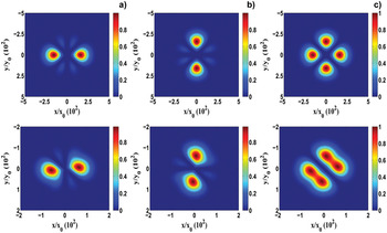
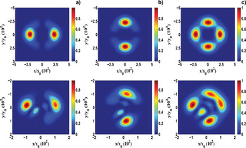
The z-component of the Poynting vector of a higher order vortex Airy beam is not presented here because of its length. According to the condition of the method of stationary phase kr = k( x 2+y 2+z 2)1/2→ ∞, we take z > 106λ in the far-field to ensure the validity of the calculated results. In the following numerical calculations, we take λ = 0.53 µm, x 0 = y 0 = 100 μm, z 0 = kx 02 = 12 cm, and x d = y d = 0. The normalized energy flux distributions of the order n = 1 and 2 vortex Airy beams (a) TE term, (b) TM term, (c) whole beam at the plane z = 50z 0 are depicted in Figures 1 and 2, respectively. Figure 1 shows the energy flux distributions on the order n = 1 vortex Airy beam with the modulation parameter a = 0.1 and 0.5, whereas Figure 2 corresponds to n = second order vortex Airy beam.
Normalized energy flux distribution of n = first order vortex Airy beam at the plane z = 50z 0 (a) TE term, (b) TM term, and (c) whole beam. Upper row, a = 0.1; lower, a = 0.5

Normalized energy flux distribution of n = second order vortex Airy beam at the plane z = 50z 0 (a) TE term, (b) TM term, and (c) whole beam. Upper row, a = 0.1; lower, a = 0.5

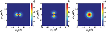
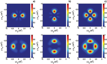
For comparison, the energy flux distributions of an Airy beam, its TE and TM terms are also depicted in Figure 3. Obviously, the TE and TM terms of the vortex Airy beam are orthogonal to each other in the far-field. As shown in the upper rows in Figures 1 and 2 for a = 0.1, the superimposition of the two lobes of energy flux distributions of TE term with that of the TM term results in the appearance of four lobes in the energy flux distributions of the whole beam. The distribution energy flux of in central parts of n = second mode in Figure 2 is weaker than that of n = first mode in Figure 1. In order to further understand how the properties of the vortex Airy beams are controlled by an Airy function, the modulation parameter, and vortex, the plots with the less value of the modulation parameter a = 0.01 for n = first and second modes are shown in Figure 4. The profile of the energy flux distribution in Figure 4 is almost similar to that of a = 0.1 in the upper rows in Figures 1 and 2. It is seen that changing the modulation parameter does not have much impacts on the vortex Airy beam for the two cases and the vortex function is the dominant part of the vortex Airy beams. When a = 0.5, the energy flux distributions of vortex Airy beams becomes distorted and asymmetrical because of the large exponential factor, as shown in the lower rows in Figures 1 and 2. The results show that the far-field properties of a vortex Airy beam can be controlled and manipulated by the Airy function, the modulation parameter, and vortex. In far-field, however, the effect of Airy function on the vortex Airy beam decreases with the increase of the propagation distance, compared to the impact of the modulation parameter and vortex (Siviloglou & Christodoulides, Reference Siviloglou and Christodoulides2007; Siviloglou et al., Reference Siviloglou, Brokly, Dogariu and Christodoulides2007). The energy flux distribution in central parts of the vortex Airy beam becomes weaker as the vortex order increases. The vortex Airy beam is distorted because of the impact of the large modulation parameters.
Normalized energy flux distribution of Airy beam at the plane z = 50z 0 with a = 0.1 (a) TE term, (b) TM term, and (c) whole beam.

Normalized energy flux distribution of vortex Airy beam with a = 0.001 at the plane z = 50z 0 (a) TE term, (b) TM term, and (c) whole beam. Upper row, n = 1; lower, n = 2

4. CONCLUSIONS
In conclusion, we have studied the far-field properties of the vortex Airy beam. The analytical TE and TM terms of a vortex Airy beam in far-field have been presented according to the vectorial structure of an electromagnetic beam. The energy flux distributions of a vortex Airy beam, the TE term and the TM term are illustrated in the far-field reference plane, which provide an intuitive picture to reveal the vectorial composition of the vortex Airy beams. The coupling between the vortex and Airy beam strongly affects the properties of the vortex and Airy beam in the far-field. The energy flux distribution in central parts of the vortex Airy beam becomes weaker with increasing vortex order. The influences of the exponential modulation factor on the energy flux distributions of a vortex Airy beam and its TE and TM terms are investigated and discussed. The vectorial structure of a vortex Airy beam is also compared with that of an Airy beam. This work provides useful information on how to spatially manipulate the properties of a vortex Airy beam in far-field by changing the vortex order and the modulation parameter. This study suggests a mechanism for the possibility of controlling the properties of a vortex Airy beam for specific applications.
ACKNOWLEDGMENTS
This work is partially supported by the State Key Program for Basic Research of China under Grant No. 2006CB921805 and the Key Project of the Education Commission of Zhejiang Province of China No. Z201120128.