1. Introduction
Compared with the natural atmospheric inflow environment, the Laval nozzle of high-speed wind tunnels normally generates acoustic disturbances that are one to two orders of magnitude higher, with amplitudes proportional to the fourth power of the Mach number (Luafer Reference Laufer1961; Beckwith & Miller Reference Beckwith and Miller1990; Schneider Reference Schneider2008). Such disparities can significantly impact the outcomes of hypersonic wind tunnel experiments, affecting phenomena such as the hypersonic boundary layer transition (Fedorov Reference Fedorov2011) and shock boundary layer interactions (Dolling Reference Dolling2001). As a result, considerable efforts have been directed towards understanding the mechanisms underlying the generation and radiation of high-speed boundary layer noise. This is essential not only for developing theoretical models based on acoustic analogy (Lighthill Reference Lighthill1954), but also for advancing modern hypersonic engineering research (Schneider Reference Schneider2008).
Experimental investigations of hypersonic turbulence statistics were initially carried out by Kovasznay (Reference Kovasznay1953), who identified vortex, entropy and acoustic disturbance sub-modes within the boundary layer using modal decomposition techniques. Later, Luafer (Reference Laufer1961) demonstrated that conventional blow-down supersonic wind tunnels exhibit free-stream noise environments dominated by acoustic radiation from turbulent boundary layers along the facility walls, especially at Mach numbers exceeding 2.5. Further research reinforced the significance of acoustic disturbances in the inflow environment (Bushnell Reference Bushnell1990; Stetson Reference Stetson1992), and pressure fluctuations caused by high-speed boundary layers have been quantitatively analysed using free-stream (Laufer Reference Laufer1964) and surface-mounted pressure sensors (Beresh et al. Reference Beresh, Henfling, Spillers and Pruett2011). While the dominance of acoustic disturbances is evident in these measurement data, the challenges of correlating them with the development of theoretical acoustic radiation models are also acknowledged (Laufer Reference Laufer1964; Duan, Choudhari & Wu Reference Duan, Choudhari and Wu2014).
Theoretical models of acoustic radiation developed by Phillips (Reference Phillips1960), Ffowcs Williams & Lighthill (Reference Ffowcs Williams and Lighthill1963) and Ffowcs Williams & Maidanik (Reference Ffowcs Williams and Maidanik1965) identify the generation of eddy Mach waves convecting supersonically relative to the free stream as the primary mechanism of acoustic radiation in boundary layer turbulence. These models emphasise the strong connection between near-wall turbulent motions, the generation of acoustic noise and the spatial evolution of these phenomena. Recent advancements in direct numerical simulation (DNS) have enabled detailed investigations of the spatial evolution of pressure fluctuations across various high-speed flow regimes, offering deeper insight into these complex interactions. For example, Duan et al. (Reference Duan, Choudhari and Wu2014) investigated the spatial structure of pressure fluctuations generated by fully developed turbulence in a Mach 2.5 turbulent boundary layer, focusing on the acoustic fluctuations radiated into the free stream. Building on this, Duan, Choudhari & Zhang (Reference Duan, Choudhari and Zhang2016) extended the study to a hypersonic boundary layer at Mach 5.86, identifying the dominant contribution of fluctuating Reynolds stress terms within the buffer layer of the boundary layer. Notably, they demonstrated a clear match in structural scales and convection velocity between the free-stream pressure structures and those near the wall, supporting the ‘eddy Mach waves’ hypothesis that free-stream acoustic radiation primarily originates from the near-wall region. Based on DNS of a quasi-two-dimensional nozzle of a wind tunnel at Mach 6, Hildebrand et al. (Reference Hildebrand, Choudhari, Deegan, Huang and Duan2022) described the spatio-temporal pressure structures of the boundary layer in a geometrically confined environment, showing that the vertical profile of pressure fluctuations scaled by mean shear stress remained consistent with that of a flat-plate case. To explore the mechanisms of noise generation, Zhang et al. (Reference Zhang, Wan, Liu, Sun and Lu2022) decomposed pressure fluctuations into fast, slow, viscous-induced and compressibility-induced components for subsonic, supersonic and hypersonic boundary layers. This decomposition linked pressure terms with other flow variables, revealing that wall cooling significantly increased pressure fluctuations near the wall, while having negligible impact on the outer boundary layer or free-stream flow.
To elucidate the mechanisms of acoustic generation and radiation, the vertical coherence of pressure structures and their relationship with near-wall velocity fields remains to be investigated. For incompressible flows, Baars, Hutchins & Marusic (Reference Baars, Hutchins and Marusic2017) identified geometrically self-similar eddy motions through linear coherence analysis between turbulence at a near-wall reference position and a travelled position in the logarithmic region, supporting the attached-eddy hypothesis proposed by Townsend (Reference Townsend1976). Additionally, their results describe the self-similarity with a streamwise/wall-normal aspect ratio of approximately 14 : 1. Baidya et al. (Reference Baidya2019) expanded this analysis to three-dimensional aspect ratios, reporting a 14 : 1 : 1 ratio in the streamwise, spanwise and wall-normal directions. For supersonic turbulent boundary layers, the streamwise/wall-normal aspect ratio of coherent structures increases to approximately 15.5, indicating a larger aspect ratio compared with lower-speed flows (Cheng & Fu Reference Cheng and Fu2022). This trend seems to suggest that higher-speed flows tend to generate more elongated structures in the streamwise direction. Further research has reinforced the presence of self-similar structures for both velocity and thermodynamic variables. For instance, Li et al. (Reference Li, Hutchins, Zheng, Marusic and Baars2022) used coherence spectrum analysis on flow variables such as the heat flux in atmospheric surface layers, confirmed the self-similarity of attached vortex structures for heat flux fields and revealed the influence of stability effects on the geometric characteristics of these structures. For the supersonic turbulent boundary layer at Mach 1.5, Cheng & Fu (Reference Cheng and Fu2022) observed that self-similar structures existed in the velocity, heat flux fields and the pressure fields. More recently, linear coherence analysis has been extended to analyse the interaction between the velocity fields and other flow variables. For example, Cheng & Fu (Reference Cheng and Fu2023) showed the velocity and temperature fields are strongly coupled at very-large-scale motions in compressible boundary layers. Regarding the velocity–pressure coupling, Baars, Dacome & Lee (Reference Baars, Dacome and Lee2024) revealed that the interactions mainly follow the structures of velocity fields for incompressible flows, regardless of Reynolds number. However, in hypersonic boundary layers, the role of compressibility in potentially modifying the mechanisms of velocity–pressure coupling remains to be investigated.
In this study, we examine the vertical coherence of velocity and pressure structures and their interactions within the hypersonic boundary layer at Mach 6, considering various wall temperatures. The linear coherence spectrum is calculated to investigate the self-similar coherent structures in the velocity and pressure fields, along with their geometric characteristics. Given that the surface temperature of hypersonic vehicles is frequently lower than the adiabatic wall temperature, wall-cooling effects can significantly modify flow characteristics (Duan, Beekman & Martin Reference Duan, Beekman and Martin2010; Liu, Huang & Wu Reference Liu, Huang and Wu2023). Therefore, we assess these effects by examining the geometric properties of coherent turbulent structures, including their inclination angles and three-dimensional aspect ratios. To reveal the underlying physics of compressible turbulence, and specifically the characteristics of local compressibility, the velocity field is decomposed into solenoidal and dilatational components following Helmholtz decomposition (Yu, Xu & Pirozzoli Reference Yu, Xu and Pirozzoli2019). Additionally, the scale dependence of the pressurevelocity coupling is investigated. Using linear stochastic estimation (LSE), the pressure signal across the boundary layer is predicted based on near-wall flow variables and their corresponding transfer kernels.
The dataset of interest is reviewed in § 2, and the methodology is illustrated in § 3. The spatial evolutions of velocity and pressure fields are investigated in § 4, and the interaction between them is discussed in § 5. The prediction of pressure field is quantified in § 6. The concluding remarks are highlighted in § 7.
Sketch of the computational domain in the
 $x$
,
 $y$
and
 $z$
directions.

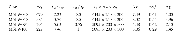
Summary of computational domain and wall parameters for the DNS database.

2. Dataset
In this study, the numerical dataset of the hypersonic boundary layer at Mach 6 is investigated at various wall temperatures, which has been described in our previous work (Liu et al. Reference Liu, Huang and Wu2023). The governing equations include the mass, momentum and total energy conservation equations which are solved by DNS using the OpenCFD code, which is widely used for supersonic (Tong et al. Reference Tong, Dong, Lai, Yuan and Li2022; Dong et al. Reference Dong, Tong, Yu, Chen, Yuan and Wang2022) and hypersonic boundary layers (Li et al. Reference Li, Tong, Yu and Li2019; Xu et al. Reference Xu, Wang, Wan, Yu, Li and Chen2021a
,Reference Xu, Wang, Wan, Yu, Li and Chen
b
, Reference Xu, Wang, Yu, Li and Chen2022a
,Reference Xu, Wang, Yu, Yu, Li and Chen
b
; Yu et al. Reference Yu, Zhou, Dong, Yuan and Xu2024). The working fluid is assumed to be a perfect gas, and the standard constitutive relations for a Newtonian fluid are employed, consistent with previous research on hypersonic pressure structures (Duan et al. Reference Duan, Choudhari and Wu2014, Reference Duan, Choudhari and Zhang2016; Zhang et al. Reference Zhang, Wan, Liu, Sun and Lu2022). Figure 1 shows the computational domain, containing the transition region, the turbulent region and the buffer region. The dataset is collected within the fully developed turbulent region. Table 1 summarises the four analysed cases with wall-to-recovery temperatures
 $T_w/T_r$
= 0.3, 0.5, 0.76 and 1 based on a recovery factor of 0.89, where the superscript
 $+$
denotes normalisation based on the inner scale. The unit Reynolds number based on free-stream quantities is set to be
 $1.08\times 10^7/m$
for all cases. The friction Reynolds number is defined as
 $Re_{\tau }=u_{\tau }\delta /\nu$
, where
 $u_{\tau }$
refers to the friction velocity,
 $\nu$
is the kinematic viscosity and
 $\delta$
denotes the boundary layer thickness. The computational domains
 $L_x$
,
 $L_y$
and
 $L_z$
are
 $1134\times 50\times 30$
mm for cases M6TW030 and M6TW050 and
 $1334\times 50\times 30$
mm for the others. For different wall-temperature cases, we will focus on the coherent structures of the hypersonic boundary layer with an adiabatic wall, and the wall-cooling effects will be accessed using the geometrical characteristics of the self-similar structures, including the inclination angle and the aspect ratio.
In our previous work, Liu et al. (Reference Liu, Huang and Wu2023) validated the mean and turbulent velocity fields and indicated good collapse with Duan et al. (Reference Duan, Choudhari and Zhang2016) for the hypersonic boundary layer at Mach 5.86 and
 $T_w/T_r=0.76$
. For the pressure fields, figure 2 compares the normalised frequency spectrum with the previous DNS dataset (Duan et al. Reference Duan, Choudhari and Zhang2016), as well as the experimental data (Huang et al. Reference Huang, Liu, Cheng and Wu2023). The comparison indicates that the current DNS captures Kolmogorov’s −7/3 scaling in the overlap region in the mediate frequencies and
 $\omega ^{-5}$
(
 $\omega$
is the frequency) scaling at high frequencies, which are consistent with the theoretical prediction (Blake Reference Blake1986) and previous experiments (Masutti et al. Reference Masutti, Spinosa, Chazot and Carbonaro2012; Huang et al. Reference Huang, Liu, Cheng and Wu2023). Besides, figure 17 (Appendix A) shows that the convection velocity of pressure fluctuations broadly agrees with the previous DNS results, showing the wall temperature exerts limited influence on the convection velocity.
Normalised frequency spectrum of pressure fields from the current DNS, compared with measured surface pressure signals (Huang et al. Reference Huang, Liu, Cheng and Wu2023) and the previous DNS simulation at Mach 5.86 (Duan et al. Reference Duan, Choudhari and Zhang2016): (a) wall; (b) free stream (
 $z/\delta =2.63$
).
 $U_{\infty}$
is the free-stream velocity and p is the pressure.

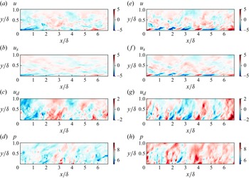
The instantaneous streamwise velocity and pressure fluctuations in the streamwise/wall-normal plane for the cases M6TW030 and M6TW100: (a, e) the original streamwise velocity field; (b, f) the solenoidal component (
 $u_s$
); (c, g) the dilatational component (
 $u_d$
); (d, h) the pressure fluctuation. Panels (a–d) refer to the case M6TW030, while (e–h) are calculated for the case M6TW100.

Throughout this paper, the Favre-averaged velocity
 $\tilde {u_i}$
, density
 $\rho$
and velocity fluctuations
 $u'_i$
will be used for the analysis and are defined as
 \begin{align} \tilde {u_i}=\frac {\overline {\rho u_i}}{\overline {\rho }}, \end{align}
 \begin{align} u'_i=u_i-\tilde {u_i}. \end{align}
We use
 $u$
,
 $v$
and
 $w$
to refer to the fluctuating velocities based on the Favre average in the streamwise (
 $x$
), wall-normal (
 $y$
) and spanwise (
 $z$
) directions, respectively. Compared with incompressible flows, a crucial aspect that complicates the modelling and prediction of hypersonic turbulence is the compressibility effects (Smits & Dussauge Reference Smits and Dussauge2006). To reveal the underlying physics of velocity–pressure couplings in the compressible turbulence and to specify the characteristic of local compressibility, the velocity field is decomposed into the solenoidal component (
 $u_s$
) and dilatational component (
 $u_d$
) according to the Helmholtz decomposition (Xu et al. Reference Xu, Wang, Wan, Yu, Li and Chen2021a
,Reference Xu, Wang, Wan, Yu, Li and Chen
b
)
 \begin{equation} u=u_s+u_d ,\end{equation}
where
 $u_s$
and
 $u_d$
satisfy
 \begin{align} \nabla \cdot u_s =0, \end{align}
 \begin{align} \nabla \times u_d =0. \end{align}
The decomposition is processed in the spectral space after the velocity field is interpolated in uniform grids. For wall-to-recovery temperature
 $T_w/T_r$
= 0.3 and 1, figures 3(a)–3(c) and 3(e–g) compare the instantaneous streamwise velocity fields with their solenoidal and dilatational components in the streamwise/wall-normal plane. The results indicate the dilatation components are organised as streamwise positive and negative alternating structures close to the wall, as previously observed in hypersonic turbulent channel flows (Yu et al. Reference Yu, Xu and Pirozzoli2019) and wall-boundary layers (Xu et al. Reference Xu, Wang, Wan, Yu, Li and Chen2021a
). By contrast, the solenoidal part roughly recovers the turbulent structures of the original velocity field, especially in the near-wall region. With the increase of wall temperatures, the turbulent structures of the streamwise velocity and its solenoidal part show rapid decrease of streamwise scale, while its dilatational streamwise velocity is less sensitive to the wall temperature. Similar to the dilatational component, figure 3(d,h) demonstrates the pressure field extends in the wall-normal direction , and its streamwise scales remain less sensitive to the wall temperature than the streamwise velocity.
3. Methodology
Recent turbulent boundary layer research has shown evidence that wall-attached vortices are self-similar in a wide range of flow configurations, including the atmospheric boundary layer (Zhang, Hu & Zheng Reference Zhang, Hu and Zheng2018; Wang, Gu & Zheng Reference Wang, Gu and Zheng2020), incompressible turbulent boundary layer (Jiménez Reference Jiménez2012; Hwang Reference Hwang2015; Baars et al. Reference Baars, Hutchins and Marusic2017; Baidya et al. Reference Baidya2019; Duan et al. Reference Duan, Zhang, Zhong, Zhu and Li2020) and compressible turbulent channel flow (Cheng & Fu Reference Cheng and Fu2022, Reference Cheng and Fu2023; Chen et al. Reference Chen, Cheng, Gan and Fu2023). Alongside the velocity components, these self-similar structures are also observed for the thermodynamic variable, particles and pressure fields (Krug et al. Reference Krug, Baars, Hutchins and Marusic2019; Cheng & Fu Reference Cheng and Fu2022; Li et al. Reference Li, Hutchins, Zheng, Marusic and Baars2022). Based on a near-wall reference position
 $y_R$
, the self-similarity of coherent structures at a travelled position
 $y$
is identified by linear coherence analysis as a function of the streamwise wavelength (
 $\lambda _x$
)
 \begin{equation} \gamma _{u}^{2}(y,y_{R};\lambda _{x})\equiv \frac {\left|\langle {\widetilde {U}(y;\lambda _{x})\widetilde {U}^{*}(y_{R};\lambda _{x})}\rangle \right|^{2}}{\left\langle {|\widetilde {U}(y;\lambda _{x})|^{2}}\right\rangle \left\langle {|\widetilde {U}(y_{R};\lambda _{x})|^{2}}\right\rangle }. \end{equation}
where
 $\widetilde {U}(y;\lambda _{x})=\mathcal {F}[u(y)]$
is the Fourier transform of
 $u(y)$
in
 $x$
(linear coherence spectrum [LCS]). The asterisk
 $*$
indicates the complex conjugate,
 $||$
designates the modulus,
 $\langle \rangle$
denotes the temporal average and the ergodic hypothesis is assumed. The statistics of the correlation map are obtained from more than 1500 snapshots of the dataset, which corresponds to
 $900 \delta / U_{\infty }$
in terms of time. Throughout the study, the reference position
 $y_R$
for the linear coherence analysis is chosen at
 $y^+ = 4$
in the near-wall region, and the choice of
 $y_R$
is found to exert negligible influence as long as
 $y_R \leqslant 15$
(Baars et al. Reference Baars, Hutchins and Marusic2017; Duan et al. Reference Duan, Zhang, Zhong, Zhu and Li2020).
While (3.1) only illustrates the linear coherence spectrum for the streamwise velocity components, the analysis will be extended to the Helmholtz-decomposed streamwise velocity and the pressure field. Baars et al. (Reference Baars, Hutchins and Marusic2017) indicated that these coherent structures within a self-similar region follow the scaling
 \begin{equation} \gamma ^{2}=C_{1}{\ln }\left ( \frac {\lambda _{x}}{\Delta y} \right ) +C_{2}, \end{equation}
where
 $\Delta y=|y-y_R|$
is the wall-normal offset, and
 $C_1\approx 0.302$
and
 $C_2\approx -0.796$
. Such constants lead to the stochastic streamwise/wall-normal aspect ratio of the flow variable
 \begin{equation} AR_{xy}=\frac {\lambda _x}{y} \bigg \rvert _{\gamma _L^2=0}=\exp {\frac {-C2}{C1}}. \end{equation}
By replacing the streamwise wavelength to spanwise scale in (3.1), the self-similar structures within the spanwise/wall-normal plane and the corresponding aspect ratio,
 $AR_{zy}$
, will be assessed.
According to the eddy Mach waves model developed by Phillips (Reference Phillips1960) and Ffowcs Williams & Lighthill (Reference Ffowcs Williams and Lighthill1963), the generation and radiation of acoustic noise are closely related to the coupling between the velocity and pressure fields. To investigate the intrinsic correlation between the near-wall velocity fields and the pressure fluctuations above, the scale dependence of their interactions is investigated by the linear coherence spectrum
 \begin{equation} \gamma _{u_i, p}^{2}(y,y_{R};\lambda _{x})\equiv \frac {\left|\langle {\widetilde {U}(y_{R};\lambda _{x})\widetilde {p}^{*}(y;\lambda _{x})}\rangle \right|^{2}}{\left\langle {|\widetilde {U}(y_{R};\lambda _{x})|^{2}}\right\rangle \left\langle {|\widetilde {p}(y;\lambda _{x})|^{2}}\right\rangle }, \end{equation}
where the velocity field
 $U(y_{R})$
is chosen at the fixed reference height in the near-wall region, while the pressure signal travels along the vertical direction.
Linear stochastic estimation provides a framework to estimate unmeasured components of a turbulent flow field using available measured quantities (Adrian Reference Adrian1979). Expanding LSE into the spectral domain, Tinney et al. (Reference Tinney, Coiffet, Delville, Hall, Jordan and Glauser2006) demonstrated its effectiveness in capturing large-scale turbulent features in the velocity and pressure fields of high-speed jets. Building on the spectral linear stochastic estimation, the present study aims to predict the pressure field across the boundary layer using near-wall pressure and velocity signals. Given the input variable near-wall pressure field,
 $p_{in}$
, the predicted off-wall pressure signal,
 $\hat {p_o}$
, is constructed from a convolution of the input signal with a first-order transfer kernel,
 $H(\lambda _{x})$
, in Fourier space
 \begin{equation} \hat {p_o}(\lambda _{x})=H(\lambda _{x})p_{in}(\lambda _{x}) ,\end{equation}
where the linear transfer kernel is defined as
 \begin{equation} H(\lambda _{x})=\frac {\phi _{p_o p_{in}}^{\prime }(\lambda _{x})}{\phi _{p_{in}p_{in}}(\lambda _{x})}. \end{equation}
where
 $\phi _{xy}^{\prime }$
is the cross-spectrum,
 $\phi _{xx}$
and
 $\phi _{yy}$
are the auto-spectral densities of signals
 $x$
and
 $y$
, respectively. For each input variable
 $x$
from the near-wall flow field, the transfer gain is intuitively scaled by the ratio of input-to-output energies (Bendat & Piersol Reference Bendat and Piersol2000; Baars, Hutchins & Marusic Reference Baars, Hutchins and Marusic2016)
 \begin{equation} |H^2(\lambda _{x})|=\gamma ^{2}(\lambda _{x})\frac {\phi _{yy}(\lambda _{x})}{\phi _{xx}(\lambda _{x})}. \end{equation}
The magnitudes of the kernel
 $ H(\lambda _{x})$
depend on the relationships between the input and output. After the kernel is computed from synchronised two-point data, a conditional estimate of the spectral output,
 $ \hat {p}_x$
, is obtained from the unconditional input. In the physical space, the conditional estimate of the off-wall pressure field correlated with the near-wall input signal is obtained by the inverse Fourier transform based on the input variable
 $x$
and the corresponding transfer kernel
 \begin{align} & \hat {p}_x=\mathcal {F}^{-1}(H \mathcal {F}[x] ). \end{align}
4. Spatial evolution of pressure fluctuations
Two-point correlation map of the streamwise velocity and pressure fields for case M6TW100, where the reference point is located at
 $y/\delta =0.05$
: (a) streamwise velocity; (b) pressure fields. The dashed lines refer to the reference inclination angles of
 $14^{\circ }$
and
 $80^{\circ }$
, respectively.

To explore the coherent structure of velocity and pressure fields, their spatial two-point correlations are examined for the adiabatic wall case as shown in figure 4. The reference height is selected in the near-wall region at
 $y/\delta =0.05$
, since the near-wall location is of primary interest for investigating the coherent structures related to wall-attached eddies. Additionally, this height corresponds to the region where turbulent kinetic energy reaches its maximum (Liu et al. Reference Liu, Huang and Wu2023). Specifically, the two-point correlation of the streamwise velocity component,
 $R_{uu}$
, is defined as
 \begin{equation} R_{uu}(\Delta {x},\Delta {y})=\frac {\left\langle u(x,y)u(x+\Delta {x},y+\Delta {y})\right\rangle }{\sigma _{u(x,y)}\sigma _{u(x+\Delta {x},y+\Delta {y})}}, \end{equation}
where
 $\Delta {x}$
and
 $\Delta {y}$
are the relative length and width from the reference point, and
 $\sigma$
indicates the temporal standard deviation. Similar analysis is extended to the pressure fields to calculate its spatial correlation
 $R_{pp}$
. Compared with the correlation maps in incompressible flows (e.g. Kim & Adrian Reference Kim and Adrian1999; Del A. et al. Reference Del Alamo, Jimnez, Zandonade and Moser2004; Hutchins & Marusic Reference Hutchins and Marusic2007), the streamwise velocity has coherent structures that have a narrower wall-normal extension of less than half of the boundary layer thickness. By contrast, figure 4(b) indicates that pressure fluctuations have a smaller streamwise structure but stronger vertical coherence. Specifically, the non-negligible positive correlation (
 $R_{pp}\gt 0.4$
) persists until the boundary layer edge. Notice that the streamwise correlation field has a larger width with increasing height, indicating that the pressure field is correlated with larger-scale structures in the free-stream flow. The increase in the streamwise length scale with height has been observed both in supersonic boundary layers at Mach 2 (Duan et al. Reference Duan, Choudhari and Wu2014) and hypersonic boundary layers at Mach 5.86 (Duan et al. Reference Duan, Choudhari and Zhang2016).
Spatial correlation of the streamwise velocity and pressure fields for case M6TW100 and the corresponding inclination angles for all cases: (a)
 $R_{uu}$
; (b)
 $R_{pp}$
; (c)
 $\alpha _{u}$
; (d)
 $\alpha _{p}$
. The streamwise shifts are identified as markers, the lighter colour and thicker line indicate the higher travelled position
 $y/ \delta \in \{0.12, 0.135, 0.15, 0.165, 0.18, 0.195, 0.21, 0.225\}$
. In (c,d), the inclination angle as a function of relative height is compared for the wall-to-recovery temperatures
 $T_w/T_r$
= 0.3, 0.5, 0.76 and 1 and the dashed lines denotes
 $14^{\circ }$
and
 $80^{\circ }$
, respectively.

To investigate the wall-temperature effects on the evolution of velocity and pressure structures, the inclination angles of coherent structures are compared for all cases. Based on the two-point correlations maps with a fixed reference point (
 $y/\delta =0.05$
), the streamwise shift that maximises
 $R_{uu}$
is identified as
 $\Delta {x^{*}}$
, and the inclination angle at each relative height
 $\Delta {y}$
is calculated as
 \begin{align} \alpha = \arctan \left(\left \langle \Delta y / \Delta x^{*} \right \rangle \right). \end{align}
Figure 5(a,b) plots the spatial correlation of the velocity and pressure fields with increasing relative heights, respectively. Accordingly, the inclination angle is calculated in figure 5(c,d). For the incompressible flows, Marusic et al. (Reference Marusic, Monty, Hultmark and Smits2013) showed that the variation of
 $\Delta {x^{*}}$
with
 $\Delta {y}$
is found to be linear, which suggests a fixed inclination angle of
 $14^{\circ }$
for the coherent structures. Comparable inclination angle is also observed for the supersonic (
 $Ma = 2$
) flows (Bross, Scharnowski & Kähler Reference Bross, Scharnowski and Kähler2021). For the hypersonic boundary layer, figure 5(c,d) indicates a roughly fixed inclination angle larger than
 $14^{\circ }$
for the adiabatic case, while it decreases to less than
 $14^{\circ }$
with decreasing wall temperature. By contrast, the inclination angle of coherent pressure structures increases with height and is less sensitive to the wall temperatures. An inclination angle around
 $80^{\circ }$
is also observed in Duan et al. (Reference Duan, Choudhari and Zhang2016).
Linear coherence spectrum at the selected heights relative to the reference height of streamwise velocity fluctuations for case M6TW100, the lighter colour and thicker and line indicate the higher travelled position for
 $20 \leqslant y^+ \leqslant 0.2Re_{\tau }$
(
 $y^+ \in \{21.63, 25.64, 32.75, 45.4\}$
): (a,d)
 $u$
; (b,e)
 $u_d$
; (c,f)
 $u_s$
. Panels (a–c) refer to the streamwise/wall-normal plane, while (d–f) are calculated in the spanwise/wall-normal plane. The lines refer to the linear fit for regions where
 $\gamma ^{2}\gt 0.1$
and
 $\lambda /\delta \lt 1$
.

Linear coherence spectrum at the selected heights relative to the reference height of pressure fluctuations for case M6TW100, the lighter colour and thicker line indicate the higher travelled position for
 $ 20\leqslant y^+ \leqslant 0.6Re_{\tau }$
(
 $y^+ \in \{24.87, 34.49, 51.61, 82.06, 136.2\}$
) in (a) and
 $ 20\leqslant y^+ \leqslant 0.4Re_{\tau }$
(
 $y^+ \in \{29.71, 39.99, 58.28, 90.8\}$
) in (b):(a) streamwise/wall-normal plane; (b) spanwise/wall-normal plane. The dashed lines are fits based on the regions where
 $\gamma ^{2}\gt 0.1$
and
 $\lambda /\delta \lt 1$
.

To further investigate the vertical coherence of these turbulent structures, the linear coherence spectra of streamwise velocity and pressure fluctuations are plotted as functions of
 $\lambda _x/\Delta y$
in figures 6 and 7, respectively. Specifically, the flow fields, including Helmholtz-decomposed velocity fields, are analysed in both streamwise/wall-normal and spanwise/wall-normal planes to investigate their three-dimensional structural aspect ratios. The near-wall reference position is chosen as
 $y^+=4$
as in Baars et al. (Reference Baars, Hutchins and Marusic2017), while the travelled positions are logarithmically spaced within the vertical range
 $ 20\leqslant y^+\leqslant 0.2Re_{\tau }$
for the streamwise velocity and a wider vertical region,
 $ 20\leqslant y^+ \leqslant 0.6Re_{\tau }$
in the streamwise/wall-normal plane and
 $ 20\leqslant y^+ \leqslant 0.4Re_{\tau }$
in the spanwise/wall-normal plane, for the pressure field. For the streamwise velocity itself, the linear coherence spectrum (LCS) collapses on one common curve that can be fitted by (3.2) in both streamwise/wall-normal and spanwise/wall-normal planes. The agreement among linear coherence spectra
 $\gamma _{u}^{2}$
suggests self-similar turbulent structures of
 $u$
. For Helmholtz-decomposed velocity fields, the LCS reveals that the dilatational component has strong vertical coherence for the entire log layer in the streamwise/wall-normal plane but much weaker vertical coherence in the spanwise/wall-normal plane. The strong vertical coherence in the
 $x{-}y$
plane is also observed in the instantaneous plot (figure 3). By contrast, the solenoidal part has a larger vertical coherent in the spanwise plane and exhibits a local peak at
 $\lambda _x/\Delta y =10$
. Notice that the rapid decrease of
 $\gamma _{u}^{2}$
with height is related to the hypersonic flow exhibiting a considerably thinner boundary layer than incompressible flows (Liu et al. Reference Liu, Huang and Wu2023). For the pressure fluctuations, figure 7 shows that the LCS collapses over a broader vertical range, particularly in the streamwise/wall-normal plane (
 $20 \leqslant y^+ \leqslant 0.6Re_{\tau }$
). Notably, the linear coherence spectrum for pressure remains larger than 0.3 at the upper edge of this region (
 $y^+ \approx 0.6Re_{\tau }$
), indicating stronger vertical coherence compared with the streamwise velocity fields.
The aspect ratios of coherent structures are assessed by fitting (3.2) based on selected regions where
 $\gamma ^{2}\gt 0.1$
and
 $\lambda /\delta \lt 1$
. The results show that the streamwise/wall-normal aspect ratio (
 $AR^{u}_{xy}\approx 16.5$
) for the streamwise velocity is relatively larger than for a range of incompressible flows (Baars et al. Reference Baars, Hutchins and Marusic2017; Baidya et al. Reference Baidya2019; Krug et al. Reference Krug, Baars, Hutchins and Marusic2019; Duan et al. Reference Duan, Zhang, Zhong, Zhu and Li2020; Li et al. Reference Li, Hutchins, Zheng, Marusic and Baars2022). A slightly larger aspect ratio than 14 is also observed for a supersonic boundary layer by Cheng & Fu (Reference Cheng and Fu2022). As for the pressure structures, a stronger wall-normal dependence is also observed in the streamwise/wall-normal aspect ratio (
 $AR^{p}_{xy}=1.6$
), which is close to
 $AR^{p}_{xy}=1.8$
for the supersonic boundary layer (Cheng & Fu Reference Cheng and Fu2022). By investigating the streamwise–spanwise LCS, Baidya et al. (Reference Baidya2019) reported that the self-similar wall-attached structures follow a three-dimensional aspect ratio of 14 : 1 : 1 in the streamwise, spanwise and wall-normal directions in high Reynolds number pipe and boundary layer flows. For the hypersonic boundary layer, figure 6(d) plots the wall-normal–spanwise linear coherence spectrum and indicates the aspect ratio as
 $AR_{zy}=1.65:1$
. The relatively larger structure in the spanwise direction thanfor incompressible flows is also observed by Bross et al. (Reference Bross, Scharnowski and Kähler2021) for the supersonic boundary layer at Mach 2 by analysing the two-point correlation and spectral calculations of the streamwise velocity fluctuations.
The aspect ratio of coherent velocity and pressure structures as a function of wall-to-recovery temperatures: (a) streamwise/wall-normal aspect ratio; (b) spanwise/wall-normal aspect ratio. The lines refer to the corresponding linear fitting.

The structural aspect ratios for the streamwise velocity and pressure coherent structures, derived from all selected datasets spanning a range of wall-to-recovery temperature ratios (
 $0.3 \leqslant T_w/T_r \leqslant 1$
), are compared in the streamwise/wall-normal and spanwise/wall-normal planes, as shown in figure 8(a,b), respectively. To analyse the variation of structural aspect ratios for the streamwise velocity and pressure coherent structures with respect to the wall temperature, the structural aspect ratio
 $AR^{i}$
is fitted using
 \begin{align} {AR^{i}= k_{i} (T_w/T_r)+b_{i}} ,\end{align}
where the subscript
 $i$
indicates the streamwise velocity component (
 $u$
), solenoidal component (
 $u_s$
), dilatational component (
 $u_d$
), slope (k), intercept (b) and pressure (
 $p$
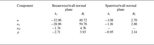
). Similar analysis is extended to the spanwise/wall-normal planes, and the key parameters are summarised in table 2. Compared with the aspect ratio that tends to hold log-linear dependence with the stability parameter for incompressible flows (Krug et al. Reference Krug, Baars, Hutchins and Marusic2019; Li et al. Reference Li, Hutchins, Zheng, Marusic and Baars2022), a linear dependence between the aspect ratio and the wall-to-recovery temperature emerges in both streamwise/wall-normal and spanwise/wall-normal planes. This relationship quantitatively supports the well-known observation that wall cooling introduces longer streamwise turbulent structures for the streamwise velocity by Duan et al. (Reference Duan, Beekman and Martin2010), who proposed the wall cooling is a sink of energy, which weakens the energy redistribution among velocity components and leads to kinetic energy accumulation in the streamwise direction. As illustrated by the instantaneous snapshots in figure 3, the streamwise velocity and its solenoidal component both show a rapid decrease in
 $k_i$
and
 $b_i$
with decreasing wall temperature, while the dilatational streamwise velocity and pressure fields exhibit much smaller streamwise/wall-normal structures. In contrast, the fitting slope and intercept have comparable magnitudes among all variable of interest in the spanwise/wall-normal plane, suggesting more similar structures in the spanwise/wall-normal plane than the streamwise/wall-normal plane.
Fitting parameters
 $k_{i}$
and
 $B_{i}$
for the streamwise (
 $u$
) velocity, solenoidal component (
 $u_s$
), dilatational component (
 $u_d$
) and pressure (
 $p$
) as a function of the wall-to-recovery temperature
 $T_w/T_r$
in streamwise/wall-normal and spanwise/wall-normal planes.

5. Coupling between the velocity and pressure fields
The previous section demonstrated that velocity and pressure fields exhibit self-similar coherent structures extending from the near-wall region to higher positions. In this section, the linear coherence spectrum is used to investigate the scale dependence of the interactions between the near-wall streamwise velocity and the pressure fields across the boundary layer. Similarly, the near-wall reference position is chosen as
 $y^+=4$
and the travelled positions are logarithmically spaced within
 $ 20\leqslant y^+\leqslant 0.2Re_{\tau }$
.
The two-point correlation map between the near-wall streamwise velocity at
 $y/\delta =0.05$
and pressure fluctuation field for case M6TW100. The dashed lines refer to the inclination angles of
 $14^{\circ }$
and
 $80^{\circ }$
for the streamwise and pressure structures, respectively. The triangle marker denotes the reference point.

Figure 9 plots the two-point correlation contour between the streamwise velocity at the reference height
 $y/\delta =0.05$
and the pressure fields above. For clarity, the inclination angles of the streamwise velocity and pressure structures are indicated. Regarding the streamwise velocity–pressure interactions, figure 9 shows that the strongest correlation aligns with the inclination angle of the streamwise velocity structures in the near-wall region. It is interesting to note that, with the increase of height to
 $y/\delta =0.5$
, the correlation begins to align more closely with the inclination angle of pressure structures and extends beyond the boundary layer thickness. The similar inclination angle highlights the increasing importance of pressure in their interactions at greater heights.
Linear coherence spectra between the pressure field and the streamwise/wall-normal velocities at the reference height
 $y^+=4$
for case M6TW100, the lighter colour line indicates the higher travelled position for
 $20 \leqslant y^+ \leqslant 0.2Re_{\tau }$
(
 $y^+ \in \{21.63, 25.64, 32.75, 45.4\}$
): (a,c) streamwise velocity; (b,d) wall-normal velocity.

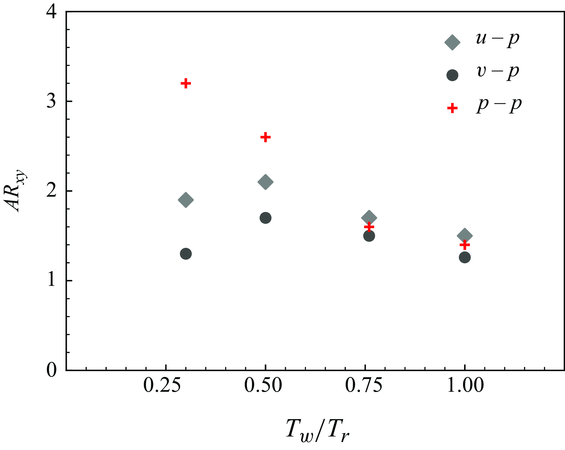
The streamwise/wall-normal aspect ratio of velocity–pressure coupling structures as a function of wall-to-recovery temperatures.

For incompressible flows, the interactions between the wall pressure and velocity fields were analysed by Baars et al. (Reference Baars, Dacome and Lee2024). They revealed that the streamwise and spanwise velocity components are coupled with the wall pressure, following the self-similar structures of the velocity fields. Specifically, the interactions emerge at a streamwise/wall-normal ratio of approximately 3 and are maximised at
 $\lambda _x/y=14$
, regardless of Reynolds number (
 $Re_\tau \approx 550-5200$
). This aspect ratio corresponds to the structural aspect ratio of wall-attached streamwise velocity, indicating that the velocity–pressure interactions follow the structures of streamwise velocity in incompressible flows. However, in compressible flows, the role of the pressure field becomes more complex due to compressibility effects. These effects result in pressure gradients being the primary driver of dilatational structures, particularly at small scales in the near-wall region (Xu, Wang & Chen Reference Xu, Wang and Chen2023).
Henceforth, the scale dependence between the near-wall velocity and the pressure fields is investigated based on the linear coherence spectrum and Helmholtz decomposition. Coherence spectra between the near-wall velocity and the pressure fields are plotted corresponding to a relatively coarse grid of
 $y$
positions that are logarithmically spaced within the logarithmic region (
 $20 \leqslant y^+ \leqslant 0.2Re_{\tau }$
). Figure 10(a) shows the interactions between the streamwise velocity and the pressure fields starting from
 $\lambda _x/ \Delta y\gt 1$
and are maximised at scales decreasing with increasing height. This reduction in interaction scale is potentially linked to the increasing influence of smaller-scale pressure structures as height increases. Notice that the interactions between streamwise velocity and pressure fields almost collapse at the aspect ratio of wall-attached streamwise velocity
 $\lambda _x/ \Delta y=16.5$
, implying that streamwise energy does not dominate the coupling. Similarly, for wall-normal velocity, the LCS in figure 10(b) shows that the interaction with pressure fields differs from that in incompressible flow, where the maximum interaction occurs at
 $\lambda _x/\Delta _y=8$
(Baars et al. Reference Baars, Dacome and Lee2024). As with streamwise velocity, the scale maximising the wall-normal velocity–pressure coupling decreases with increasing height. Based on Helmholtz decomposition, LCS is also calculated to investigate the scale dependence of interactions between the dilatational/solenoidal components and pressure term in figure 10(c,d). Notably, while the dilatational streamwise velocity shares a similar structural aspect ratio to the pressure structures, figure 10(c) shows that the solenoidal component exhibits stronger interactions with the pressure fields at small-scale motions (
 $\lambda _x/\Delta y \lt 10$
). In contrast, at larger scales, the dilatational component demonstrates stronger interactions with the pressure field, with coherence increasing with height. For the wall-normal velocity, both dilatational and solenoidal components exhibit greater coherence with the pressure field at large scales, although the solenoidal component also shows local peaks at smaller scales.
In the hypersonic boundary layer at different wall temperatures, wall-cooling effects on velocity–pressure coupling are analysed by examining the structures’ streamwise/wall-normal aspect ratio. As shown in figure 11, the velocity–pressure coupling exhibits a decreasing aspect ratio (
 $AR_{xy}$
) as wall temperature increases, except for case M6TW030. Notably, in the M6TW076 and M6TW100 cases, both streamwise and wall-normal velocity components coupled with the pressure at an aspect ratio close to that of the pressure structures, highlighting the critical role of pressure fields. However, in the M6TW030 and M6TW050 cases, the observed discrepancies in structural aspect ratios between the pressure and velocity–pressure coupling indicate that wall cooling can significantly influence the dominance of pressure in the coupling process.
6. Estimation of off-wall pressure fields
(a) Contour plots of the transfer kernel
 $H_p^2$
for the pressure signal for case M6TW100, with decreasing values represented by lighter shades of dashed grey lines. Contour line levels range from 0.1 to 1 with an increment of 0.1. (b) Same as (a), but at selected heights.

In hypersonic wind tunnel facilities, acoustic noise is a primary contributor to free-stream disturbances, making its evaluation critical for experimental studies. Previous findings indicate that the pressure field remains self-correlated throughout the boundary layer, while its correlation with velocity fields is strongest at smaller scales. Based on near-wall pressure and velocity signals, this section applies LSE to predict the pressure field across the boundary layer.
Figure 12 plots the kernel of linear gain that takes the near-wall pressure signal to predict the pressure field above,
 $H_p^2$
, as a function of relative heights. The reference point is located in the near-wall region (
 $y^+ =4$
). As suggested by Baars et al. (Reference Baars, Hutchins and Marusic2016), the gain function can be interpreted as an experimentally calculated scale filter such that scaling the transfer kernel gain allows for the prediction of a filter that retains only the coherent scales of the acquired input. As demonstrated in the linear kernel analysis of flow variables for incompressible and compressible flows (Cheng & Fu Reference Cheng and Fu2022; Li et al. Reference Li, Hutchins, Zheng, Marusic and Baars2022), the transfer kennel of the pressure term also presents higher values at larger wavelengths and lower wall-normal offsets present higher values. As suggested by the linear coherence spectrum, figure 12(a) shows a slow decay of the linear kernel, indicating a strong vertical coherence of the pressure fields. Specifically, the linear gain at large scales remains greater than 0.5 above half of the boundary layer thickness. At the selected heights (
 $z/\delta = 0.1, 0.5, 1$
), figure 12(b) presents line plots of the transfer kernel, illustrating a decreasing range of coherent scales with increasing height. Nonetheless, the transfer kernel retains non-negligible values for
 $\lambda _x / \delta \gt 1$
at
 $y / \delta = 1$
.
By contrast, figure 13 reveals that the linear gain between near-wall velocity components and pressure fields does not increase at larger wavelengths, indicating that the estimations are confined to small-scale motions. Specifically, the linear gain kernel
 $H_u^2$
shows that the transfer from the near-wall streamwise velocity to the pressure field above is primarily concentrated at scales smaller than the boundary layer thickness (
 $\lambda _x / \delta$
) and decreases to less than 0.1 at
 $y / \delta \gt 0.3$
. Similarly, while the wall-normal component exhibits transfer across a slightly broader range of scales, its transfer kernel,
 $H_v^2$
, also decays rapidly with height.
Contour plots of
 $H_{u_i}^2$
for the pressure signal based on near-wall velocity fields for case M6TW100, with decreasing values represented by lighter shades of dashed grey lines.

The observed (grey), large-scale filtered (black) and LSE-predicted pressure field at selected heights for case M6TW100: (a)
 $y/\delta = 0.1$
; (b)
 $y/\delta = 0.5$
; (c)
 $y/\delta = 1$
.

At three selected heights along the boundary layer (
 $y/\delta = 0.1, 0.5, 1$
), figure 14 compares the instantaneous pressure signals and their linear stochastic predictions (
 $\hat {p}$
). The predicted pressure fields are obtained by applying LSE based on inputs of near-wall pressure (
 $\hat {p}_p$
), streamwise velocity (
 $\hat {p}_u$
) and wall-normal velocities (
 $\hat {p}_v$
) at
 $y^+=4$
. The low-pass filter filters the original pressure field with the cutoff scale equal to the boundary layer thickness, which is denoted as
 $\tilde {p}$
. As suggested by the kernel of linear gain, only the predicted pressure fields based on the near-wall pressure and its kernel capture the large-scale motions of the original signal. Specifically, the LSE based on near-wall pressure signal inputs can capture majority fluctuations at
 $y/\delta = 0.1$
, showing the predicted pressure roughly overlaps with the filtered original field. With the height increase to
 $y/\delta = 0.5$
and 1, the predicted pressure only recovers the large-scale trends, as the transfer kernel is limited on large scales. By contrast, figure 14 shows the predicted pressure with the velocity fields as input variables fails to follow the large-scale motions of the original field, only the small-scale fluctuations are partially recovered at
 $y/\delta = 0.1$
. To better compare the spectral distribution of the observed and predicted pressure fields, the premultiplied energy spectra of the conditional estimate at the selected heights (
 $y/\delta = 0.1, 0.5, 1$
) are shown in figure 15. The energy spectra are time averaged for the entire dataset to ensure the convergence. As shown in the instantaneous pressure fields (figure 14), the LSE based on the near-wall pressure field,
 $\hat {p}_p$
, closely resembles the pressure field at
 $y/\delta =0.1$
while the other predictions underestimate the energy magnitude. With increase of height, only the LSE predictions based on near-wall pressure signal are able to capture the large-scale energy at the same magnitude, while for the other predictions the linearly estimated spectrum constitutes less energy due to the lack of perfect coherence (the visual implication of (3.6)).
The observed and linear stochastic estimation-predicted premultiplied spectra of the pressure field normalised by the square of shear stress
 $\tau _w$
at selected heights for case M6TW100: (a)
 $y/\delta = 0.1$
; (b)
 $y/\delta = 0.5$
; (c)
 $y/\delta = 1$
.

Spatial correlation between the original fields filtered by large-scale filter with the LSE-predicted signal based on different input variables and the corresponding transfer kernel for case M6TW100.

In figure 16, the spatial correlation between the large-scale filtered and LSE-predicted pressure fields is calculated across the boundary layer as a function of height. The LSE fields are derived based on near-wall pressure, velocity and Helmholtz-decomposed velocity fields. Among all the input variables, the near-wall pressure yields the strongest LSE, with the correlation coefficient
 $C_{p,\hat{p}}$
approaching 0.8 at the first reference point and gradually decreasing to 0.4 at the boundary layer edge. This result indicates that large-scale off-wall pressures are reasonably well represented by the near-wall pressure signal, which can be captured by wall-mounted pressure sensors. When using velocity fields as input, the dilatational wall-normal velocity exhibits the spatial correlation of 0.4 with the original pressure field in the near-wall region, but this correlation diminishes to near zero with increasing height. The relatively stronger correlation between the LSE-predicted pressure based on the dilatational velocity component
 $u_d$
and the original pressure fields is likely related to the significant role that dilatational components play in near-wall self-sustaining cycles (Yu et al. Reference Yu, Zhou, Dong, Yuan and Xu2024).
7. Summary and conclusions
This project aims to investigate the vertical coherence of the pressure field and its coupling with velocity components in turbulent hypersonic boundary layers at various wall-to-recovery temperatures. The study first confirms the presence of self-similar coherent structures in the streamwise velocity, Helmholtz-decomposed streamwise velocity and pressure fields, examining both the streamwise/wall-normal and spanwise/wall-normal planes. Main findings are summarised as follows.
-
(i) For the hypersonic boundary layer with an adiabatic wall, the streamwise velocity exhibits coherent structures with streamwise/wall-normal/spanwise aspect ratios of 16.5 : 1 : 1.65. This streamwise/wall-normal aspect ratio exceeds the 15.5 : 1 ratio observed for supersonic cases (Cheng & Fu Reference Cheng and Fu2022) and the 14:1 ratio seen in incompressible cases (Baars et al. Reference Baars, Dacome and Lee2024), indicating that the aspect ratio largely increases with Mach number.
-
(ii) Based on Helmholtz decomposition, the results show the dilatational component has a much smaller streamwise/wall-normal aspect ratio than, and comparable spanwise/wall-normal aspect ratio to, the solenoidal component.
-
(iii) In comparison with the velocity fields, the linear coherence spectra indicate that pressure fields exhibit linear coherence spectra larger than 0.4 until
 $y\approx 0.6 Re_{\tau }$
. The collapse of the linear coherence spectra suggests a three-dimensional structural aspect ratio of 1.6 : 1 : 1.2.
-
(iv) Regarding wall-cooling effects, both velocity and pressure fields exhibit a linear increase of the streamwise/wall-normal and spanwise/wall-normal aspect ratios as wall temperatures decrease, providing a quantitative description of the elongation of streamwise structures caused by a cooled wall (Duan et al. Reference Duan, Beekman and Martin2010).

These findings suggest the validity of the attached-eddy hypothesis for the high-speed turbulent boundary layer and highlights the modified geometrical characteristics from incompressible to hypersonic boundary layers in the context of varying wall temperatures in high-speed flows.
This study examines the coupling between near-wall velocity and pressure signals and the pressure field across the boundary layer, identifying two major distinctions from incompressible flow velocity–pressure coupling. First, the solenoidal component exhibits stronger interactions with the pressure fields in the near-wall region, while the dilatational component has stronger interactions with the pressure field at large scales with the increase of height. Second, in hypersonic flow regimes, pressure fields play a more dominant role. For instance, two-point correlation maps indicate that the strongest interactions occur along the inclination angle of coherent pressure structures. Furthermore, spectral analysis demonstrates that velocity–pressure coupling generally adheres to the pressure field’s distance-from-the-wall scaling, except in scenarios involving cooled walls. Furthermore, spectral LSE and linear transfer gain analysis reveal a pronounced vertical coherence in the pressure field at large scales, whereas the transfer gain with velocity components remains confined to smaller scales. This strong vertical coherence indicates that pressure input data are particularly effective for reconstructing off-wall pressure fields, outperforming other near-wall input variables. These findings demonstrate that off-wall pressure structures, which are coherent with near-wall fields, can be estimated using near-wall signals measurable via wall-mounted pressure sensors. These results provide a valuable foundation for assessing off-wall flow properties using wall-mounted sensors, with potential applications in future wind tunnel experiments. Future analyses can explore the relationship between the vertical coherence of pressure structures and their convection velocity in high-speed flows at different Mach numbers, where variations in convection speed arise from changes in compressibility effects.
Declaration of interests.
The authors declare that they have no conflict of interest.
Appendix A. Convection velocity
The convection velocity for a range of wall-to-recovery temperatures at selected heights, compared with the previous DNS study at Mach 5.86 (Duan et al. Reference Duan, Choudhari and Zhang2016): (a) wall; (b)
 $y/\delta = 0.158$
; (c)
 $y/\delta =0.734$
; (d)
 $y/\delta =1.571$
.

Following the calculation in Kim (Reference Kim1989) and Duan et al. (Reference Duan, Choudhari and Zhang2016)of the propagation speed of pressure fluctuations, figure 17 shows
 $U_c$
calculated based on a spatial and temporal decay (
 $\Delta x$
and
 $\Delta t$
) that satisfies
 \begin{equation} \frac {\partial R_{pp}(r_x, \Delta t)}{\partial r_x }\Big |_{ \ r_x = \Delta x } = 0, \end{equation}
where the space–time correlation of the pressure field,
 $R_{pp} (\Delta x, \Delta t)$
, is defined as
 \begin{equation} R_{pp}(\Delta {x},\Delta {t})=\frac {\left\langle u(x,y)u(x+\Delta {x},y+\Delta {y})\right\rangle }{\sigma _{u(x,y)}\sigma _{u(x+\Delta {x},y+\Delta {y})}} ,\end{equation}
where
 $\sigma$
indicates the temporal standard deviation.