





1. Introduction
Low-frequency instabilities driven by various sources of energetic particles (EPs), such as auxiliary heating and fusion-born alpha particles, have been widely observed in previous experiments (McGuire et al. Reference McGuire1983; Heidbrink et al. Reference Heidbrink, Strait, Doyle, Sager and Snider1991, Reference Heidbrink, Strait, Chu and Turnbull1993; Wong et al. Reference Wong1991; Kimura et al. Reference Kimura1998; Sharapov et al. Reference Sharapov2002; Nazikian et al. Reference Nazikian2008; Breizman & Sharapov Reference Breizman and Sharapov2011) and theoretically investigated (Chen, White & Rosenbluth Reference Chen, White and Rosenbluth1984; Berk et al. Reference Berk, Dam, Borba, Candy, Huysmans and Sharapov1995; Zonca, Chen & Santoro Reference Zonca, Chen and Santoro1996; Fu et al. Reference Fu, Nazikian, Budny and Chang1998; Heidbrink et al. Reference Heidbrink, Ruskov, Carolipio, Fang, Zeeland and James1999; Berk et al. Reference Berk, Borba, Breizman, Pinches and Sharapov2001; Gorelenkov, Pinches & Toi Reference Gorelenkov, Pinches and Toi2014; Chen & Zonca Reference Chen and Zonca2016). These instabilities can lead to the degradation of EP confinement and potential damage to the first wall of devices. In particular, as we approach the realisation of fusion ignition, the instabilities in the presence of fusion product–alpha particles under burning plasma conditions have become a primary concern. Some basic alpha physics and alpha-driven Alfvén instabilities have been generally introduced by Heidbrink (Reference Heidbrink2002, Reference Heidbrink2008). Furthermore, analytical investigations or numerical simulations of linear Alfvén eigenmode (AE) stability and their parameter dependences have been done by evaluating wave–particle resonant drives and principal damping mechanisms (Gorelenkov et al. Reference Gorelenkov, Berk, Budny, Cheng, Fu, Heidbrink, Kramer, Meade and Nazikian2003; Rodrigues et al. Reference Rodrigues, Figueiredo, Ferreira, Coelho, Nabais, Borba, Loureiro, Oliver and Sharapov2015; Tolman et al. Reference Tolman, Loureiro, Rodrigues, Hughes and Marmar2019).
The toroidal Alfvén eigenmodes (TAEs) were first predicted by Cheng et al. in the last century (Cheng, Chen & Chance Reference Cheng, Chen and Chance1985; Cheng & Chance Reference Cheng and Chance1986), then TAEs were identified in the Tokamak Fusion Test Reactor (TFTR) during neutral beam injection (Wong et al. Reference Wong1991), and subsequent experimental observations and numerical simulations have demonstrated its capability to induce significant EP transport and losses (Hsu & Sigmar Reference Hsu and Sigmar1992; Sigmar et al. Reference Sigmar, Hsu, White and Cheng1992; Todo & Sato Reference Todo and Sato1998). The analytical formulations of contributions from EPs to the perturbative kinetic energy – accordingly, the growth rate of TAE instabilities – were derived (Fu, Cheng & Wong Reference Fu, Cheng and Wong1993; Breizman & Sharapov Reference Breizman and Sharapov1995; Fülöp et al. Reference Fülöp, Lisak, Kolesnichenko and Anderson1996). Motivated by these findings, we use a simplified perturbative physical model to derive an energy exchange formula via wave–particle resonances to numerically calculate the kinetic drive or damping, and therefore to investigate the linear stability of TAEs in burning plasmas. This approach can significantly circumvent the constraints of time and computing resources imposed by global simulations when exploring large ranges of parameter space, while the study of parameter dependences is important for experimental design and modelling to identify key parameters and instability trends for later more detailed analyses.
With advancements in auxiliary heating systems and enhancements of plasma confinement, plasma temperatures can exceed tens of
 $\mathrm{keV}$
for sustaining the thermonuclear fusion (Shimada et al. Reference Shimada2007). Simultaneously, high magnetic field operation scenarios have been proposed in response to the recent advancements of high-temperature superconducting technology and the pursuit of compact, cost-effective devices. By keeping the plasma beta or fusion triple product constants, the dependences of TAE linear instability on bulk temperature and magnetic field strength will be studied in this work.
The remainder of this paper is organised as follows. Section 2 presents a detailed derivation of the numerical formulae employed in this study. The linear stability of core-localised TAEs and global TAEs, along with their dependences on key parameters such as plasma temperature and magnetic field, are investigated in §§ 3 and 4, respectively. Finally, the summary and further discussions are presented in § 5.
2. Physical model
In this section, after calculations of TAE mode structures by solving the ideal magnetohydrodynamics (MHD) shear Alfvén wave (SAW) equations, we use the quadratic form of the momentum equation to evaluate the growth rate contributions from both EPs and thermal ions. Combined with the radiative damping (Berk, Mett & Lindberg Reference Berk, Mett and Lindberg1993; Fu et al. Reference Fu, Cheng, Budny, Chang, Darrow, Fredrickson, Mazzucato, Nazikian, Wong and Zweben1996; Breizman & Sharapov Reference Breizman and Sharapov2025) and trapped electron collisional damping (Fu & Cheng Reference Fu and Cheng1992; Gorelenkov & Sharapov Reference Gorelenkov and Sharapov1992; Gorelenkov et al. Reference Gorelenkov, Berk, Budny, Cheng, Fu, Heidbrink, Kramer, Meade and Nazikian2003) rates from analytical formulae, we directly assess the linear stability of TAEs and their parameter dependences.
2.1. Calculation of TAE mode structures
Starting from the ideal SAW equations, by considering coupling between
 $m$
and
 $m+1$
poloidal harmonics for a fixed toroidal mode number
 $n$
due to toroidal effects (Berk et al. Reference Berk, Dam, Guo and Lindberg1992), the following equations were derived under the approximations of circular flux surfaces and large aspect ratio (Berk et al. Reference Berk, Dam, Borba, Candy, Huysmans and Sharapov1995):
 \begin{align} \frac {\mathrm{d}}{\mathrm{d}y}\left [(y+1/2)^2-\varOmega ^2\right ]\frac {\mathrm{d}\delta \varPhi _m}{\mathrm{d}y}&-\frac {1}{s^2}\left [(y+1/2)^2-\varOmega ^2\right ]\delta \varPhi _m-\left (\varOmega ^2(2\epsilon +\varDelta ^{\prime })+\frac {\varDelta ^{\prime }}{4}\right )\frac {\mathrm{d}^2\delta \varPhi _{m+1}}{\mathrm{d}y^2} \nonumber\\[4pt] &+\frac {1}{s^2}\left [\varOmega ^2(\epsilon -\varDelta ^{\prime })-\frac {1}{4}(\epsilon +\varDelta ^{\prime })+\alpha /2\right ]\delta \varPhi _{m+1}=0,\nonumber\\[4pt] \frac {\mathrm{d}}{\mathrm{d}y}\left [(y-1/2)^2-\varOmega ^2\right ]\frac {\mathrm{d}\delta \varPhi _{m+1}}{\mathrm{d}y}&-\frac {1}{s^2}\left [(y-1/2)^2-\varOmega ^2\right ]\delta \varPhi _{m+1}-\left (\varOmega ^2(2\epsilon +\varDelta ^{\prime })+\frac {\varDelta ^{\prime }}{4}\right )\frac {\mathrm{d}^2\delta \varPhi _m}{\mathrm{d}y^2} \nonumber\\[4pt] &+\frac {1}{s^2}\left [\varOmega ^2(\epsilon -\varDelta ^{\prime })-\frac {1}{4}(\epsilon +\varDelta ^{\prime })+\alpha /2\right ]\delta \varPhi _m=0,\nonumber\\[-4pt] \end{align}
where
 $\delta \varPhi _m,\,\delta \varPhi _{m+1}$
are the perturbed electrostatic potentials with poloidal mode number
 $m$
and
 $m+1$
, respectively. The radial coordinate is defined as
 $y\equiv n[q-q(r_m)]$
, with
 $r_m$
being the radius of the TAE gap location and
 $\varOmega \equiv \omega /2\omega _0$
is the frequency normalised to
 $\omega _0=v_A(r_m)/2q(r_m)R_a$
. The equilibrium parameters include the magnetic shear
 $s\equiv \mathrm{d}(\ln q)/\mathrm{d}(\ln r)$
, the normalised pressure gradient
 $\alpha \equiv -R_aq^2\mathrm{d}\beta /\mathrm{d}r$
, the inverse aspect ratio
 $\epsilon \equiv r/R_a$
and the radial derivative of Shafranov shift
 $\varDelta ^\prime =\mathrm{d}\Delta /\mathrm{d}r$
. Here,
 $R_a$
is the major radius at magnetic axis. All these parameters are evaluated at
 $r=r_m$
, where
 $q(r_m)=(2m+1)/2n$
, based on the assumption that these two harmonics are localised near the TAE gap location.
To solve this eigenequation for the TAE eigenvalues and eigenfunctions, we discretise the radial variable
 $y$
and perturbed potential
 $\delta \varPhi$
to transform the coupled equations into the standard matrix eigenvalue problem
 $[\textsf{A}_{2N\times 2N}+\omega ^2\textsf{B}_{2N\times 2N}] \boldsymbol{\varPhi }_{2N}=0$
. In this formulation, the block band matrices
 $\textsf{A}$
and
 $\textsf{B}$
both have the diagonal blocks and non-diagonal blocks. The diagonal blocks represent the terms related with each poloidal
 $\delta \varPhi _m$
, while the non-diagonal blocks account for the coupling with
 $\delta \varPhi _{m+1}$
and
 $\delta \varPhi _{m-1}$
. To investigate the global TAE structures, we generalise these coupled equations with two harmonics to a multi-
 $m$
coupling system, so the matrix
 $\textsf{A}$
or
 $\textsf{B}$
can be written as
 \begin{align} \left ( \begin{array}{c@{\quad}c@{\quad}c@{\quad}c@{\quad}c} \textsf{S}_{\boldsymbol{{m-2}}} & \textsf{C} & 0 & 0 & 0 \\[3pt] \textsf{C} & \textsf{S}_{\boldsymbol{{m-1}}} & \textsf{C} & 0 & 0\\[3pt] 0 & \textsf{C} & \textsf{S}_{\boldsymbol{m}} & \textsf{C} & 0 \\[3pt] 0 & 0 & \textsf{C} & \textsf{S}_{\boldsymbol{{m+1}}} & \textsf{C} \\[3pt] 0 & 0 & 0 & \textsf{C} & \textsf{S}_{\boldsymbol{{m+2}}} \end{array} \right ) \left ( \begin{array}{c} \boldsymbol{\varPhi ^{m-2}} \\[2pt] \boldsymbol{\varPhi ^{m-1}} \\[2pt] \boldsymbol{\varPhi ^{m}} \\[2pt] \boldsymbol{\varPhi ^{m+1}} \\[2pt] \boldsymbol{\varPhi ^{m+2}} \end{array} \right ) . \end{align}
Here,
 $\textsf{S}$
and
 $\textsf{C}$
are both
 $N\times N$
band matrices. We use the MATLAB function eigs to numerically solve the eigenfrequency
 $\omega$
and the radial mode structure
 $\delta \varPhi (y)$
with the eigenfrequency limited to TAE gap accumulation points, as given analytically by
 \begin{align} \omega _{-}=\sqrt {\frac {1}{1+\hat {\epsilon }}}\frac {v_A(r_m)}{2q(r_m)R_a}\leqslant \omega \leqslant \omega _{+}=\sqrt {\frac {1}{1-\hat {\epsilon }}}\frac {v_A(r_m)}{2q(r_m)R_a}, \end{align}
where
 $\hat {\epsilon }\approx 2(\epsilon +\varDelta ^\prime )$
denotes the toroidal coupling factor and zero-boundary conditions are assumed. Among two-
 $m$
coupled core-localised TAE solutions, two distinct types of modes are identified (Berk et al. Reference Berk, Dam, Borba, Candy, Huysmans and Sharapov1995; Fu Reference Fu1995; Candy et al. Reference Candy, Breizman, Dam and Ozeki1996): even TAEs, those with frequencies just above the lower accumulation points (
 $\omega _-$
) and even-symmetric mode structures
 $\delta \varPhi _m\approx \delta \varPhi _{m+1}$
; and odd TAEs, with frequencies just below the upper accumulation points (
 $\omega _+$
) and odd-symmetric mode structures
 $\delta \varPhi _m\approx -\delta \varPhi _{m+1}$
.
2.2. Hybrid model
In this framework, the total perturbed pressure tensor in the momentum equation is decomposed into a fluid part, arising from the summation of the fluid-described species and the adiabatic responses of the perturbed distribution function
 $\delta f$
for kinetic-described species, and a kinetic part from the non-adiabatic responses:
 $\delta {\textsf{ P}}=\delta {\textsf{ P}}_f{\textsf{ I}}+\delta {\textsf{ P}}_k$
. Consequently, the linearised momentum equation is expressed as
 \begin{align} \rho \frac {\mathrm{d}^2\boldsymbol{\xi }}{\mathrm{d}t^2} = -\boldsymbol{\boldsymbol{\nabla }}\delta {\textsf{ P}}_f-\boldsymbol{\boldsymbol{\nabla }}\boldsymbol{\cdot }\delta {\textsf{ P}}_k-\frac {1}{4\pi }(\delta \boldsymbol{B}\times \boldsymbol{\boldsymbol{\nabla }}\times \boldsymbol{B}+\boldsymbol{B}\times \boldsymbol{\boldsymbol{\nabla }}\times \delta \boldsymbol{B}), \end{align}
where the perturbed electromagnetic fields satisfy the following relations:
 \begin{align} &\delta \boldsymbol{B} = \boldsymbol{\boldsymbol{\nabla }}\times (\boldsymbol{\xi }\times \boldsymbol{B}), \nonumber\\[5pt] &\delta \boldsymbol{E}_\perp = \mathrm{i}\omega \boldsymbol{\xi }\times \boldsymbol{B}/\mathrm{c}, \end{align}
where
 $\boldsymbol{\xi }$
is the plasma displacement. The perturbed distribution function is separated into adiabatic and non-adiabatic components:
 $\delta f=\delta f_{ad}+\delta g$
, where
 $\delta g$
is governed by the linearised gyro-kinetic equation:
 \begin{align} (\partial _t+v_\parallel \partial _\parallel +\boldsymbol{v}_d\boldsymbol{\cdot }\boldsymbol{\boldsymbol{\nabla }})\delta g=\mathrm{i}e\boldsymbol{Q}F_0\mathrm{J_0}\delta L. \end{align}
The operator
 $\boldsymbol{Q}F_0\equiv (\omega -\omega _*)\partial _EF_0$
represents the phase-space gradients of the equilibrium distribution function
 $F_0$
;
 $\mathrm{J_0}(k_\perp \rho )$
is the zero-order Bessel function and
 $\delta L$
represents the effective perturbed potential
 \begin{align} \delta \boldsymbol{E} = -\boldsymbol{\boldsymbol{\nabla }}\delta L = -\boldsymbol{\boldsymbol{\nabla }}(\delta \varPhi -v_\parallel \delta A_\parallel /\mathrm{c}). \end{align}
The perturbed parallel electromagnetic fields,
 $\delta E_\parallel = -\boldsymbol{\nabla} _\parallel \delta L$
and
 $\delta B_\parallel$
, are neglected for SAW instabilities. In calculating the kinetic response, the wave–particle energy exchange comes from primarily the particles’ magnetic drift motion. So, we could rewrite the
 $\delta L$
term as below in the following equation:
 \begin{align} \delta L = \frac {\mathrm{i}}{\omega }\boldsymbol{v}_d\boldsymbol{\cdot }\delta \boldsymbol{E}_\perp . \end{align}
Here,
 $\boldsymbol{v}_d$
and
 $\omega _*$
denote the magnetic drift velocity and the diamagnetic drift frequency, respectively, which are defined as
 \begin{align} \boldsymbol{v}_d&\equiv \boldsymbol{b}\times \frac {\left (({1}/{2})v_\perp ^2\boldsymbol{\boldsymbol{\nabla }}\ln B+v_\parallel ^2\boldsymbol{\kappa }\right )}{\varOmega _c} ,\nonumber\\[4pt] \omega _*&\equiv -n\partial _{P_\phi }F_0/\partial _EF_0. \end{align}
2.3. Quadratic formula
Here, we take an inner product of (2.4) with the adjoint vector of the perturbed displacement
 $\boldsymbol{\xi ^\dagger }$
and integrate all over the plasma volume to obtain a quadratic form:
 \begin{align} \delta W_f+\delta W_k-\omega ^2\delta I = 0, \end{align}
where the Fourier expression
 $\boldsymbol{\xi }=\boldsymbol{\xi }(\boldsymbol{x})\mathrm{e}^{-\mathrm{i}\omega t}$
is used. We have the detailed expressions for the potential terms:
 \begin{align} \delta I &=\int \mathrm{d}^3\boldsymbol{x}\rho |\boldsymbol{\xi }|^2, \nonumber\\[3pt] \delta W_f &=\int \mathrm{d}^3\boldsymbol{x}\boldsymbol{\xi }^\dagger \boldsymbol{\cdot }\left (\boldsymbol{\boldsymbol{\nabla }}\delta P_f+\frac {1}{4\pi }(\delta \boldsymbol{B}\times \boldsymbol{\boldsymbol{\nabla }}\times \boldsymbol{B}+\boldsymbol{B}\times \boldsymbol{\boldsymbol{\nabla }}\times \delta \boldsymbol{B})\right ), \nonumber\\[3pt] \delta W_k &=\int \mathrm{d}^3\boldsymbol{x}\boldsymbol{\xi }^\dagger \boldsymbol{\cdot }(\boldsymbol{\boldsymbol{\nabla }}\boldsymbol{\cdot }\delta \mathcal{P}_k). \end{align}
Apparently,
 $\delta I$
and
 $\delta W_f$
are from the ideal MHD equation, while the latter includes the fluid responses from particles;
 $\delta W_k$
represents the kinetic responses from particles.
With the assumption of perturbative kinetic effects, we expand the eigenfrequency and the eigenfunction in terms of a small parameter order by order:
 $\omega =\omega _0+\omega _1,\,\boldsymbol{\xi }=\boldsymbol{\xi _0}+\boldsymbol{\xi _1}$
. So, the zero-order equation of (2.10) is
 \begin{align} \delta W_f(\boldsymbol{\xi}_{\boldsymbol{0}}^\dagger ,\boldsymbol{\xi _0})-\omega _0^2\delta I(\boldsymbol{\xi}_{\boldsymbol{0}}^\dagger ,\boldsymbol{\xi _0})=0, \end{align}
which is the expression of the ideal MHD energy principle and can be used to find the eigenfrequency and eigenfunction. The first-order equation is
 \begin{align} \delta W_f(\boldsymbol{\xi}_{\boldsymbol{0}}^\dagger ,\boldsymbol{\xi _1})-\omega _0^2\delta I(\boldsymbol{\xi}_{\boldsymbol{0}}^\dagger ,\boldsymbol{\xi _1})-2\omega _0\omega _1\delta I(\boldsymbol{\xi}_{\boldsymbol{0}}^\dagger ,\boldsymbol{\xi _0})+\delta W_k(\boldsymbol{\xi}_{\boldsymbol{0}}^\dagger ,\boldsymbol{\xi _0})=0. \end{align}
The former two terms are cancelled due to the self-adjointness of the ideal MHD operators:
 $\delta W_f(\boldsymbol{\xi}_{\boldsymbol{0}}^\dagger ,\boldsymbol{\xi _1})-\omega _0^2\delta I(\boldsymbol{\xi}_{\boldsymbol{0}}^\dagger ,\boldsymbol{\xi _1})=\delta W_f(\boldsymbol{\xi}_{\boldsymbol{1}}^\dagger ,\boldsymbol{\xi _0})-\omega _0^2\delta I(\boldsymbol{\xi}_{\boldsymbol{1}}^\dagger ,\boldsymbol{\xi _0})=0$
, the last two terms give the modification of the eigenfrequency due to kinetic effects:
 \begin{align} \omega _1=\frac {\delta W_k(\boldsymbol{\xi}_{\boldsymbol{0}}^\dagger ,\boldsymbol{\xi _0})}{2\omega _0\delta I(\boldsymbol{\xi}_{\boldsymbol{0}}^\dagger ,\boldsymbol{\xi _0})}. \end{align}
Furthermore, we give the explicit expression for
 $\delta W_k$
 \begin{align} \delta W_k &= -\int \mathrm{d}^3\boldsymbol{x}\int \mathrm{d}^3\boldsymbol{v}(\delta E_k)^\dagger \delta g \nonumber\\[3pt] &= -e\int \mathrm{d}^3\boldsymbol{x}\int \mathrm{d}^3\boldsymbol{v}\left (\frac {\mathrm{i}}{\omega }\mathrm{J_0}\boldsymbol{v}_d\boldsymbol{\cdot }\delta \boldsymbol{E}_\perp \right )^{\!\dagger} \delta g, \end{align}
with
 $\delta E_k$
being the energy exchanged between wave and particles. The
 $\delta g$
can be calculated through the gyro-kinetic equation (2.6):
 $\delta g=\mathrm{i}e\boldsymbol{Q}F_0(\partial _t+v_\parallel \partial _\parallel +\boldsymbol{v}_d\boldsymbol{\cdot }\boldsymbol{\boldsymbol{\nabla }})^{-1}(({\mathrm{i}}/{\omega })\mathrm{J_0}\boldsymbol{v}_d\boldsymbol{\cdot }\delta \boldsymbol{E}_\perp )\equiv \mathrm{i}e\boldsymbol{Q}F_0\boldsymbol{P}^{-1}(({\mathrm{i}}/{\omega })\mathrm{J_0}\boldsymbol{v}_d\boldsymbol{\cdot }\delta \boldsymbol{E}_\perp )$
, with
 $\boldsymbol{P^{-1}}$
being the inverse propagator. For the dimensionless definition of
 $G\equiv ({e}/{2E\omega })\mathrm{J_0}\boldsymbol{v}_d\boldsymbol{\cdot }\delta \boldsymbol{E}_\perp$
and the corresponding Fourier expansion
 $G=\hat {G}(r,\,\theta )\mathrm{e}^{\mathrm{i}(n\phi -\omega t)}$
, we have
 \begin{align} \delta W_k &= -e\int \mathrm{d}^3\boldsymbol{x}\int \mathrm{d}^3\boldsymbol{v}\left (\frac {\mathrm{i}}{\omega }\mathrm{J_0}\boldsymbol{v}_d\boldsymbol{\cdot }\delta \boldsymbol{E}_\perp \right )^\dagger \boldsymbol{P}^{-1}\mathrm{i}e\boldsymbol{Q}F_0\left (\frac {\mathrm{i}}{\omega }\mathrm{J_0}\boldsymbol{v}_d\boldsymbol{\cdot }\delta \boldsymbol{E}_\perp \right ) \nonumber\\ &= -4\mathrm{i}\int \mathrm{d}^3\boldsymbol{x}\int \mathrm{d}^3\boldsymbol{v}E^2\boldsymbol{Q}F_0G^\dagger \boldsymbol{P}^{-1}G. \end{align}
We employ the integration along the unperturbed particle orbit to solve the
 $\boldsymbol{P^{-1}}$
. The toroidal angle can be divide into a secular term and a periodic function of particle orbit
 $\phi (t)=\langle \dot {\phi }\rangle t+\tilde {\phi }(t)\equiv \omega _\phi t+\tilde {\phi }(t)$
with
 $\omega _\phi$
being the averaged toroidal frequency, and we carry out the Fourier transformation
 $\hat {G}(r,\,\theta )\mathrm{e}^{\mathrm{i}n\tilde {\phi }}=\sum _p \hat {G_p}(r)\mathrm{e}^{-\mathrm{i}p\omega _\theta t},$
 $\hat {G_p}(r)=({1}/{\tau _b})\int \hat {G}(r,\,\theta )\mathrm{e}^{\mathrm{i}(p\omega _\theta t+n\tilde {\phi })}\mathrm{d}t$
with the orbit-averaged poloidal frequency
 $\omega _\theta =\langle \dot {\theta }\rangle$
and the transit or bounce period in the poloidal direction
 $\tau _b=2\pi /\omega _\theta$
. Then,
 $\boldsymbol{P^{-1}}G$
is given by
 \begin{align} \boldsymbol{P}^{-1}G &= \int _{-\infty }^{t}\mathrm{d}t^{\prime }G \nonumber\\[3pt] &= \int _{-\infty }^{t}\mathrm{d}t^{\prime }\sum _p\hat {G_p}(r)\mathrm{e}^{\mathrm{i}(n\omega _\phi - p\omega _\theta -\omega )t^{\prime }} \nonumber\\[3pt] &= \sum _p\hat {G_p}(\bar {r})\frac {\mathrm{e}^{\mathrm{i}(n\omega _\phi - p\omega _\theta -\omega )t}}{\mathrm{i}(n\omega _\phi - p\omega _\theta -\omega )}. \end{align}
The transformation of the phase space variables to the constants of motion and magnetic surface coordinates is
 \begin{align} \int \mathrm{d}^3\boldsymbol{x}\int \mathrm{d}^3\boldsymbol{v} &= \int J_r(\psi _p,\theta,\phi )\mathrm{d}\psi _p\mathrm{d}\theta \mathrm{d}\phi \sum _{\sigma _\parallel }\int J_E(E,\varLambda,\phi )\mathrm{d}E\mathrm{d}\varLambda \mathrm{d}\phi \nonumber\\[3pt] &= \sum _{\sigma _\parallel }\frac {4\pi ^2}{m^2}\int E\frac {r}{q}\mathrm{d}r\mathrm{d}t\mathrm{d}E\mathrm{d}\varLambda . \end{align}
We have the velocity-space Jacobian
 $J_E(E,\,\varLambda ,\,\phi )=BE/(m^2B_av_\parallel )$
with the pitch angle parameter
 $\varLambda \equiv \mu B_a/E$
and the magnetic field at the magnetic axis
 $B_a$
. Here, we use the relation
 $({\mathrm{d}\theta }/{\mathrm{d}l_\parallel })=({(\boldsymbol{B}\boldsymbol{\cdot }{\boldsymbol{\nabla }}\theta )}/{B})=({(1/J_r)}/{B})$
and
 $({J_rB\mathrm{d}\theta}/{v_\parallel })=({\mathrm{d}l_\parallel }/{v_\parallel })=\mathrm{d}t$
to transform to the time integral. By taking (2.18) and (2.17) back to (2.16) and (2.14), and the perturbative assumption
 $\omega _1\sim \omega _i\ll \omega _0\sim \omega _r$
, the kinetic contributions to the TAE linear growth rate from particles are finally written as
 \begin{align} \gamma =\omega _1 &= \frac {\mathrm{Im}(\delta W_k)}{2\omega _0\delta I} \nonumber\\[3pt] &= \frac {1}{2\omega _0\delta I}\frac {16\pi ^3}{m^2}\sum _{\sigma _\parallel ,\,p}\int \left . \frac {r}{q}E^3\partial _EF_0(\omega -\omega _*)\tau _b|\hat {G_p}|^2(p\,{\rm d}pE)^{-1}\mathrm{d}r\mathrm{d}\varLambda \right |_{E=E_{resonance}} \end{align}
with the definition that
 $E_{resonance}$
is the particle energy satisfying the wave–particle resonant conditions and
 $p{\rm d}pE\equiv |\partial (n\omega _\phi -p\omega _\theta -\omega )/\partial E|$
. This formula is similar to the one derived by Fu et al. (Reference Fu, Cheng and Wong1993) except for the inclusion of finite Larmor radius (FLR) effects through the Bessel function
 $\mathrm{J_0}$
in
 $G_p$
, and is the same with the one of Fülöp et al. (Reference Fülöp, Lisak, Kolesnichenko and Anderson1996) except for the formal differences.
For calculating the orbit harmonic term
 $G_p$
in the aforementioned integration, with a given resonance order
 $p$
and characteristic particle values: radial location
 $r$
and pitch angle parameter
 $\varLambda$
; we can calculate the resonant energy
 $E_{resonance}$
from the resonant condition
 $\omega =n\omega _\phi -p\omega _\theta$
. Particles are categorised into passing particles and trapped particles with different assumptions used to calculate
 $\omega _\phi$
and
 $\omega _\theta$
, and the separatrix pitch angle value is chosen as
 $\hat {\varLambda }\equiv B_a/B_{max}(r)$
to distinguish them:
 $0\to \hat {\varLambda }$
representing the passing particles, while
 $\hat {\varLambda }\to \varLambda _{max}\equiv B_a/B_{min}(r)$
representing the trapped particles.
When the triplet
 $(r, \varLambda , E)$
are ascertained (for passings,
 $\mathrm{sign}(v_\parallel )$
should be also taken into consideration), we perform orbit-following until they complete a full poloidal circuit:
 \begin{align} \frac {\mathrm{d}r}{\rm{d}t} &= -v_d\sin \theta, \nonumber\\[3pt]\frac {\mathrm{d}\theta }{\rm{d}t} &= \left (\frac {v_\parallel }{qR}-\frac {v_d\cos \theta }{r}\right ), \nonumber\\[3pt] \frac {\mathrm{d}\phi }{\rm{d}t} &= \frac {v_\parallel }{R} ,\nonumber\\[3pt] \frac {\mathrm{d}v_\parallel }{\rm{d}t} &=-\frac {\mu \boldsymbol{b}\boldsymbol{\cdot }\boldsymbol{\boldsymbol{\nabla }}B}{m}\approx -\frac {\varLambda E}{m}\frac {r\sin \theta }{qR^2}. \end{align}
Then,
 $G_p$
can be expressed with a more explicit formation:
 \begin{align} G_p=\frac {1}{\tau _b}\int _t\sum _m\left (v_d\sin \theta \delta \varPhi _m^\prime -\frac {\mathrm{i}m}{r}v_d\cos \theta \delta \varPhi _m\right )\mathrm{J_0}(k_\perp \rho )\mathrm{e}^{\mathrm{i}(p\omega _\theta t+n\tilde {\phi }-m\theta )}\mathrm{d}t, \end{align}
where each value can be calculated through (2.20) and then can be averaged. The resolutions are
 $n_r=200$
with radial ranges based on the mode widths and
 $n_l=32$
with the pitch angle having the range:
 $0\to \varLambda _{max}$
. Finite Larmor radius (FLR) and finite Orbit width (FOW) effects are included.
2.4. Benchmark with the ITPA n = 6 TAE case
In this subsection, we choose the ITPA
 $n=6$
core-localised TAE case as the benchmark (Könies et al. Reference Könies2018). It is a hydrogen background plasma with deuterium as EP under concentric circular magnetic surfaces. The basic parameters are as follows: the major radius
 $R_0=10\,\mathrm{m}$
, the minor radius
 $a=1\,\mathrm{m}$
and magnetic field
 $B_a=3\,\mathrm{T}$
. All the densities and temperatures of the particle species are assumed to be constants with Maxwellian distribution functions:
 $n_e=n_i=2\times 10^{19}\,\mathrm{m^{-3}},\:T_e=T_i=1\,\mathrm{keV}$
, except for the EP density profile that is given by
 \begin{align} n_h(r)=7.5135\times 10^{16}\exp \big({-}0.6664\tanh \big(\big(\sqrt {r/a}-0.49123\big) /0.198739\big)\big)\,\mathrm{m^{-3}}. \end{align}
The safety factor profile is
 $q(r)=1.71+0.16(r/a)^2$
, where
 $r$
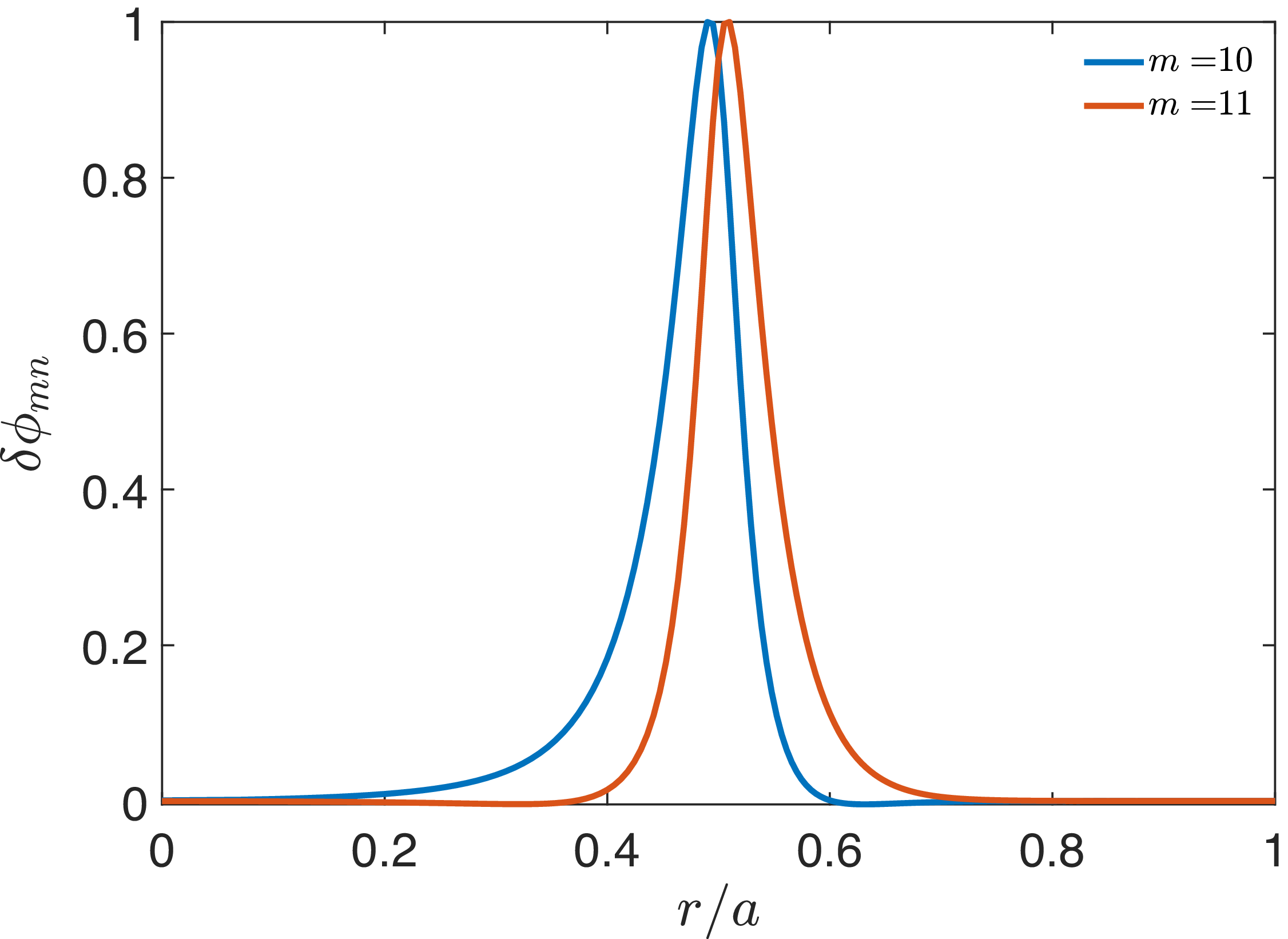
represents the square root of the toroidal magnetic flux. Our numerical solution yields the eigenfrequency
 $\omega _0=4.05\times 10^5\,\mathrm{rad\,s^{-1}}$
and eigenfunction as shown in figure 1, both of which are in great agreement with those results of Könies et al. (Reference Könies2018)
ITPA
 $n=6$
TAE mode structure calculated from (2.1).

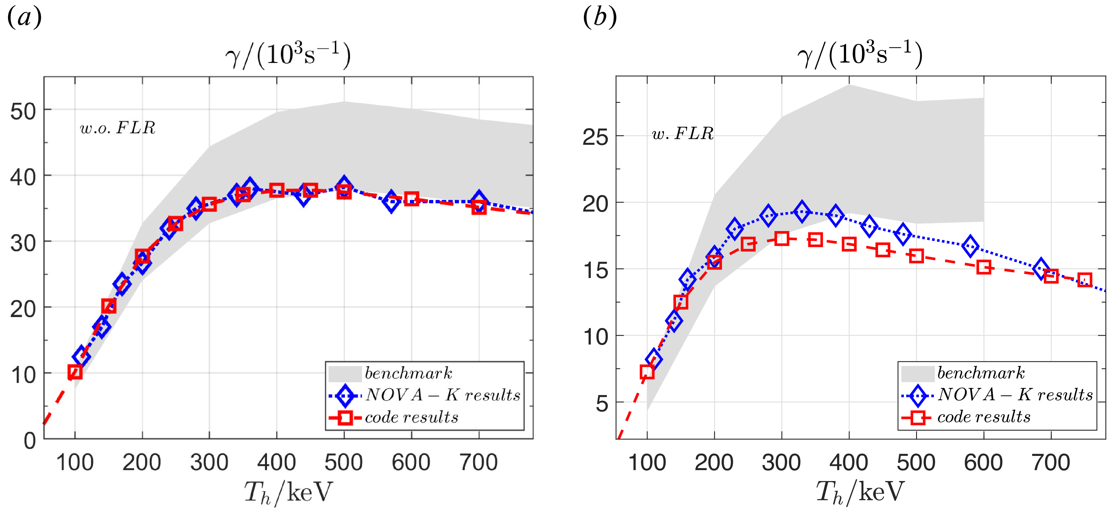
According to the integral formula prescribed in last subsection, we calculate the drives from EPs under different EP temperatures with and without the FLR effect. The results are shown in figure 2. The
 $v_\parallel =\pm v_A/3$
and
 $v_\parallel =\pm v_A/5$
resonances are identified to be the major contributions to destabilise the TAE, which is consistent with the results from HMGC and MEGA codes (Könies et al. Reference Könies2018). In the absence of FLR effects, our results show high consistency with the NOVA-K code, reflecting the similarity in our underlying physical models. NOVA-K is an eigenvalue code based on a hybrid model with perturbative EP kinetic effects. The quantitative discrepancies between our results and those from other codes stem from the distinction between perturbative and non-perturbative models. When FLR effects are included, the small differences with NOVA-K results at higher EP temperatures may arise from the different calculation methods of the Bessel function
 $\mathrm{J_0}$
as FLR effects become more important.
Growth rates from EPs (a) without and (b) with FLR effects: red lines for our results, blue lines for NOVA-K and grey zones for all the other codes of Könies et al. (Reference Könies2018).

3. Linear stability of core-localised TAEs in ITER
In this section, we consider the ITER baseline scenario, which originates from Shimada et al. (Reference Shimada2007), to investigate the linear stability of core-localised TAEs with circular surfaces assumption. The basic parameters are given by
 $R_0=6\,\mathrm{m},\, a=2\,\mathrm{m},$
 $B_a=5\,\mathrm{T},\,\beta _b(0)=6.4\,\%,\,n_i(r)=10^{20}\,\mathrm{m^{-3}},\,n_e=n_i+e_hn_h$
. Electron temperature has the same profile with bulk plasma pressure
 $P(r)=P(0)[1-(r/a)^2]$
,
 $T_e(r)=T_e(0)[1-(r/a)^2]$
and
 $T_e(0)=20\,\mathrm{keV}$
, so the ion temperature is given by
 $T_i=(P-n_eT_e)/n_i$
. The effective bulk ion mass is
 $m_i=2.5m_p$
. Alpha particles are the only EP species with birth energy
 $E_{\alpha ,0}=3.5\,\mathrm{MeV}$
and density profile
 \begin{align} n_\alpha (r)=n_\alpha (0)\left (\frac {P(r)}{P(0)}\right )^{7/2}. \end{align}
Here,
 $n_\alpha (0)$
is calculated by
 $n_\alpha = n_Dn_T\langle \sigma v\rangle \tau _s = n_i^2\langle \sigma v\rangle \tau _s/4$
with slowing-down time
 $\tau _{s,\,\alpha }=3.704[\mathrm{s}](T_e[\mathrm{10\,keV}])^{({3}/{2})}/n_e[10^{19}\,\mathrm{m^{-3}}]$
(Cordey Reference Cordey1976) and reactivity rate (Atzeni & ter Vehn Reference Atzeni and ter Vehn2004)
 \begin{align} \langle \sigma v\rangle _{DT} = 9.1\times 10^{-22}\exp \left (-0.572\left |\ln \frac {T[\mathrm{keV}]}{64.2}\right |^{2.13}\right )\,\mathrm{m^3}\,\mathrm{s}^{-1}. \end{align}
The effective alpha beta is therefore written as
 $\beta _{\alpha 0}=n_{\alpha 0}T_{\alpha 0}$
with
 $T_{\alpha 0}$
representing the effective averaged kinetic energy. The slowing-down distribution function is chosen for alpha particles
 \begin{align} f_\alpha =\frac {n_\alpha (r)}{c\big(v^3+v_c^3\big)} \end{align}
with critical velocity
 \begin{align} v_c=\left (\frac {3\sqrt {\mathrm{\pi }}m_e}{4m_i}\right )^{1/3}\left (\frac {2T_e}{m_e}\right )^{1/2}. \end{align}
This formula is derived from Gaffey (Reference Gaffey1976) with the parameter simplification
 $Z_1=\sum _i({n_iZ_i^2m_b}/{n_em_i})=({n_iZ_i^2m_b}/{n_em_i})\approx ({m_b}/{m_i})$
; here, we consider the mixed deuterium–tritium plasma with
 $Z_i=1$
and use the quasi-neutral approximation
 $n_i\approx n_e$
. Maximum velocity is defined as
 $v_{\alpha ,0}=\sqrt {2E_{\alpha ,0}/m_\alpha }$
and
 $c$
is the normalisation constant.
In burning plasma regimes, the primary damping mechanisms for SAW instabilities are Landau damping (Fu & Dam Reference Fu and Dam1989; Betti & Freidberg Reference Betti and Freidberg1992; Zonca Reference Zonca1993) from bulk ions, trapped electron collisional damping (Fu & Cheng Reference Fu and Cheng1992; Gorelenkov et al. Reference Gorelenkov, Berk, Budny, Cheng, Fu, Heidbrink, Kramer, Meade and Nazikian2003) and radiative damping (Berk et al. Reference Berk, Mett and Lindberg1993; Fu et al. Reference Fu, Cheng, Budny, Chang, Darrow, Fredrickson, Mazzucato, Nazikian, Wong and Zweben1996; Breizman & Sharapov Reference Breizman and Sharapov2025) arising from coupling with kinetic shear Alfvén waves (KSAW). The electron Landau damping is neglected since the electron thermal velocity exceeds the Alfvén velocity by an order of magnitude and, from the numerical calculations, we find that it is negligible with the value several orders of magnitude smaller than the ion Landau damping. In the subsequent numerical investigations of linear TAEs stability, the Landau damping is calculated through (2.19) while the radiative damping is determined via the following analytical formulation (Fu et al. Reference Fu, Cheng, Budny, Chang, Darrow, Fredrickson, Mazzucato, Nazikian, Wong and Zweben1996; Breizman & Sharapov Reference Breizman and Sharapov2025):
 \begin{align} \gamma _{rad}=-\frac {1}{3}\hat {\epsilon }\frac {\omega _{TAE}^3}{\omega ^2}\big(1-h_m^2\big)\exp \left (-\frac {2}{\sqrt {\eta _m}}I_1(h_m)\right ), \end{align}
where
 \begin{align} h_m &= 2(\omega ^2-\omega _{-}^2)/(\omega _{+}^2-\omega _{-}^2)-1, \nonumber\\ I_1(h_m)&=\int _{0}^{\sqrt {1+h_m}}\mathrm{d}x\sqrt {(1-(h_m-x^2)^2)}, \nonumber\\ \eta _m &=8n^2s^2q_m^2\frac {\rho _s^2}{\hat {\epsilon }^3r_m^2}. \end{align}
Here,
 $\rho _s^2=({T_i}/{m_i\varOmega _c^2})(({3}/{4})+({T_e}/{T_i}))$
is related to the ion gyroradius and sound gyroradius;
 $\omega _{TAE}\equiv v_A(r_m)/2q_m R_a$
and
 $\omega$
are the analytical TAE frequency and the calculated frequency, respectively. Additionally,
 $\omega _\pm$
are the upper/lower accumulation points with definitions in (2.3),
 $h_m$
represents the relative location of TAE in the continuum gap and
 $h_m=\pm 1$
corresponds respectively to the upper and lower tip of the gap. Furthermore, the trapped electron collisional damping is directly calculated by using (2.5)–(2.6) of Gorelenkov et al. (Reference Gorelenkov, Berk, Budny, Cheng, Fu, Heidbrink, Kramer, Meade and Nazikian2003). The net growth rate is determined by the summation of alpha drive and dampings:
 $\gamma =\gamma _\alpha +\gamma _{lan,i}+\gamma _{rad}+\gamma _{col}$
.
3.1. Mode structures
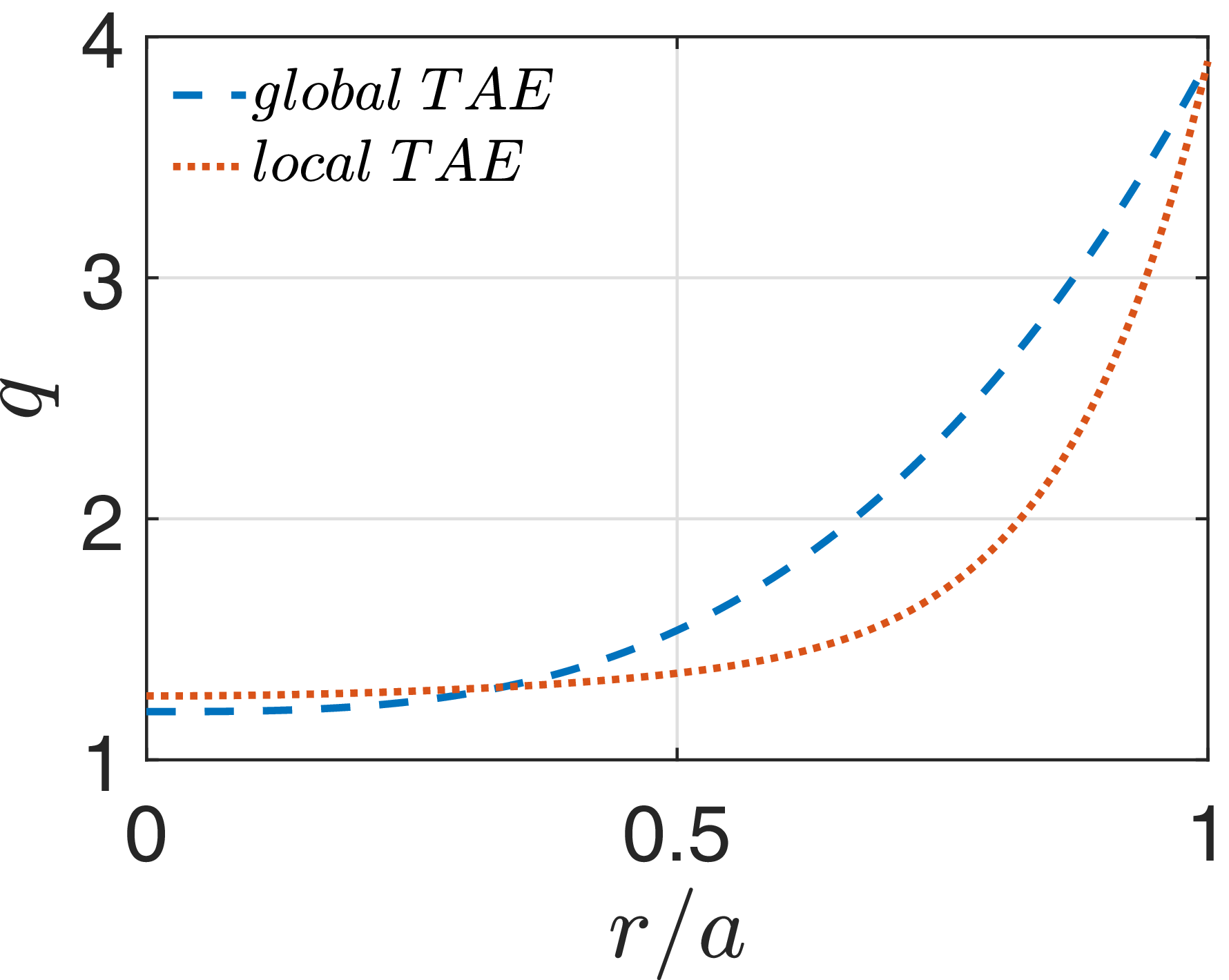
A slightly flattened
 $q$
-profile near the core is adopted to facilitate the investigations of core-localised TAEs, with the comparison illustrated in figure 3. The plasma densities are reduced from the ITER values listed earlier to give a lower plasma beta
 $\beta _{b}=5.44\,\%$
for core-localised TAEs, thereby preventing TAE frequencies from merging into the Alfvén continuum at higher plasma betas. The corresponding parameters for alpha particles are the slowing-down time
 $\tau _{\alpha ,s}\approx 1.5\,\mathrm{s}$
, the core density
 $n_{\alpha 0}\approx 7.5\times 10^{17}\,\mathrm{m^{-3}}$
and the effective alpha particle beta
 $\beta _{\alpha }=1.16\,\%$
.
Two safety factor profiles used for core-localised and global TAE calculations.

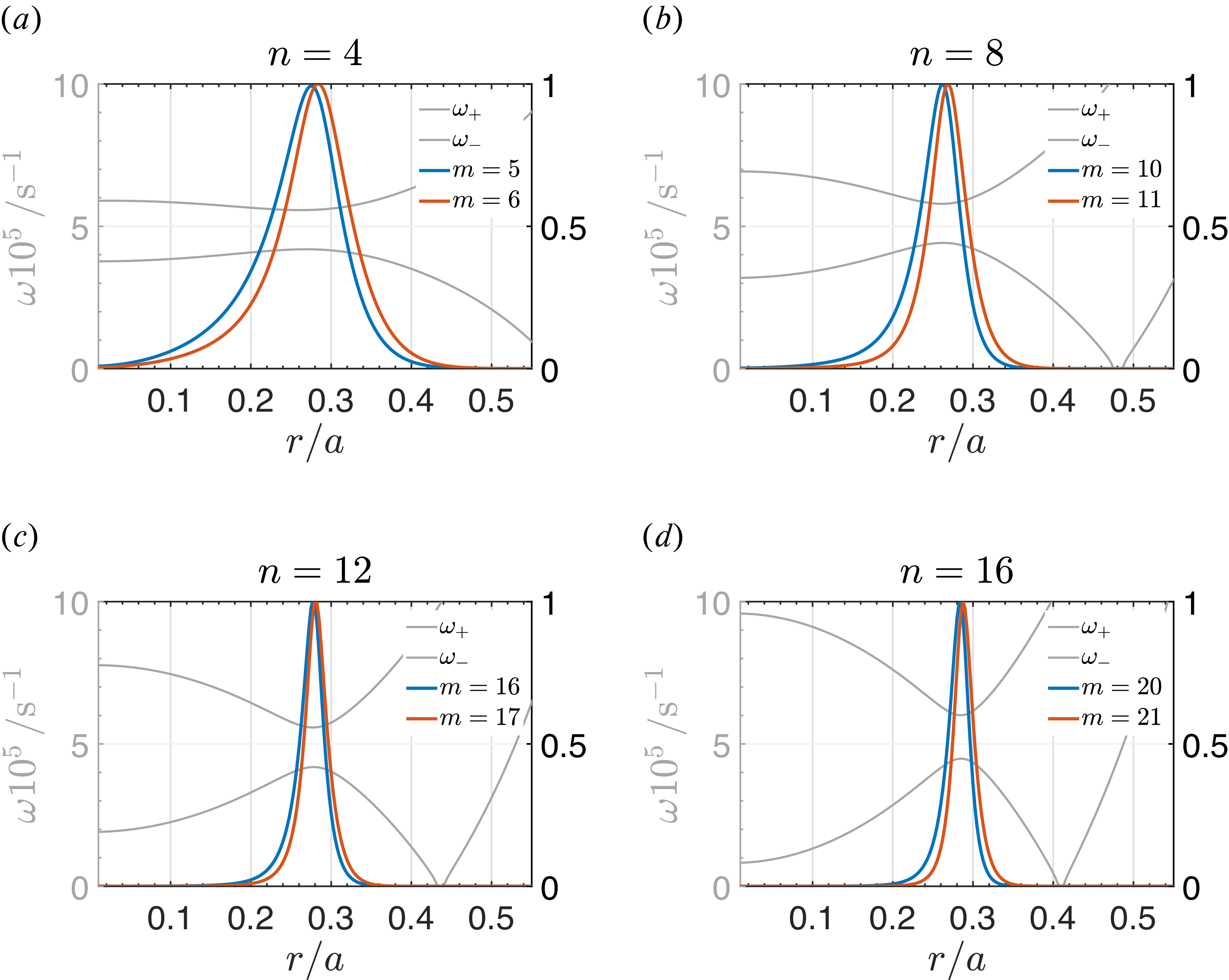
Even core-localised TAEs with mode number
 $n = (a)$
4, (b) 8, (c) 12 and (d) 16.

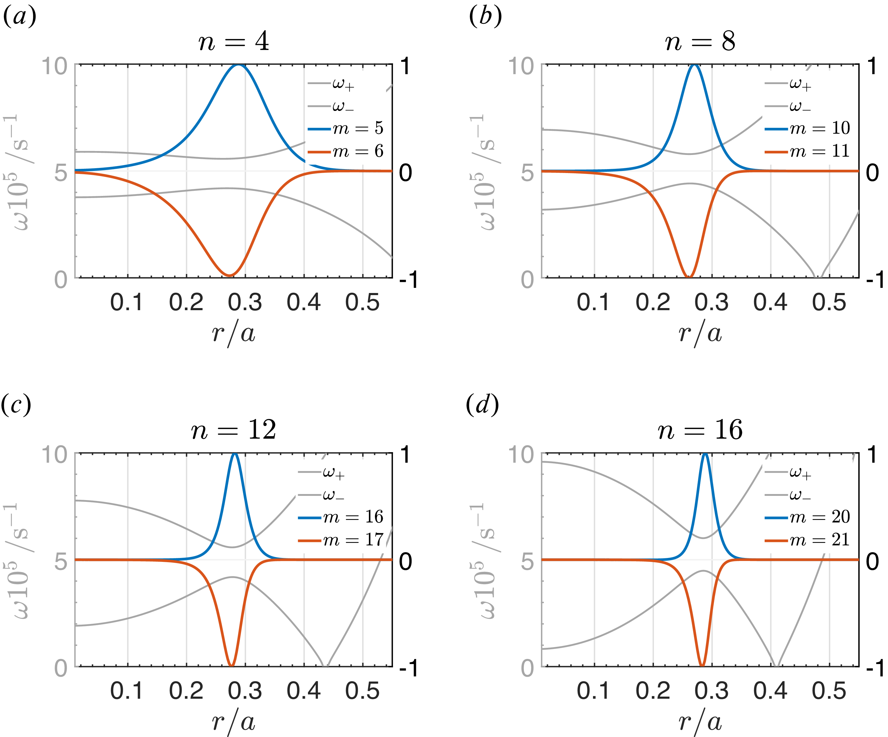
Odd core-localised TAEs with mode number
 $n = (a)$
4, (b) 8, (c) 12 and (d) 16.

Figure 5. Long description
Panel A: A line graph shows the frequency (omega) as a function of the normalized radial position (r/a) for mode numbers n = 4. The vertical axis represents the frequency in units of 10^5 s^-1, and the horizontal axis represents the normalized radial position. The graph includes lines for different mode numbers (m = 5 and m = 6) and shows the behavior of omega+ and omega-. Panel B: A line graph shows the frequency (omega) as a function of the normalized radial position (r/a) for mode numbers n = 8. The vertical axis represents the frequency in units of 10^5 s^-1, and the horizontal axis represents the normalized radial position. The graph includes lines for different mode numbers (m = 10 and m = 11) and shows the behavior of omega+ and omega-. Panel C: A line graph shows the frequency (omega) as a function of the normalized radial position (r/a) for mode numbers n = 12. The vertical axis represents the frequency in units of 10^5 s^-1, and the horizontal axis represents the normalized radial position. The graph includes lines for different mode numbers (m = 16 and m = 17) and shows the behavior of omega+ and omega-. Panel D: A line graph shows the frequency (omega) as a function of the normalized radial position (r/a) for mode numbers n = 16. The vertical axis represents the frequency in units of 10^5 s^-1, and the horizontal axis represents the normalized radial position. The graph includes lines for different mode numbers (m = 20 and m = 21) and shows the behavior of omega+ and omega-.
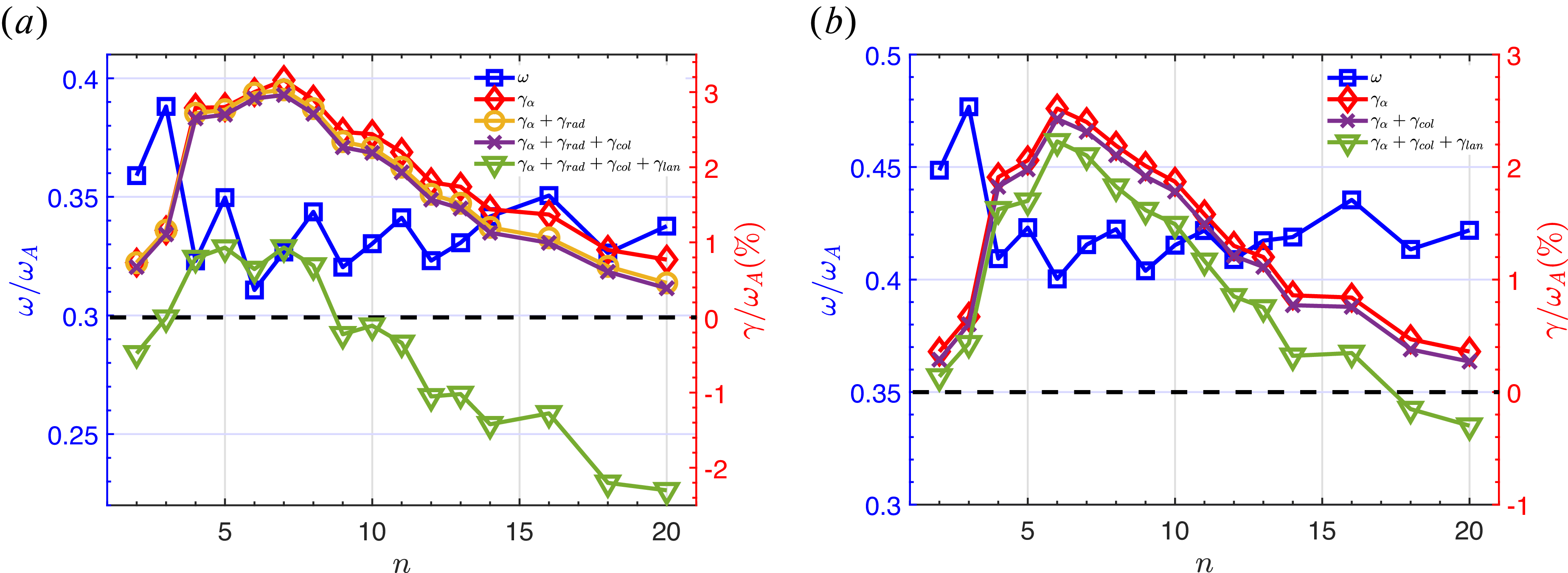
Mode structures with different toroidal mode numbers are shown in figures 4 and 5 for even TAEs and odd TAEs. The corresponding growth rates and frequencies are plotted in figure 6. As
 $n$
varies, the relative scale between the radial mode width and the particle orbit width changes, which results in the increase or decrease of the growth rate with increasing mode number. Most unstable mode numbers are around
 $n=6$
. From the nearly linear fitting of EP drive versus EP beta (finding
 $\beta _{\alpha ,c}(\gamma _\alpha =\gamma _d)$
), we determine that the corresponding beta thresholds for these unstable TAEs are
 $\beta _{\alpha ,c}\approx 0.74\,\%$
for even TAE and
 $0.09\,\%$
for odd TAE. When considering the radiative damping arising from coupling to the KSAWs, there is an apparent difference between even TAEs and odd TAEs. In contrast to even TAEs with ballooning-type mode structures of which two non-overlapping KSAWs propagate radially away from each other, KSAWs associated with odd TAEs propagate radially towards each other and form an overlapping pattern within the TAE localisation region. This results in a negligibly small energy flux loss and significantly lower damping rate (Nyqvist & Sharapov Reference Nyqvist and Sharapov2012), for which we neglect the
 $\gamma _{rad}$
for the odd TAE cases. At a fixed background beta, the Landau damping is highly sensitive to the resonant velocity, which is directly determined by the mode frequency. The odd TAEs exhibit higher mode frequencies, shifting their resonances into a velocity space region with lower damping contributions. Consequently, this leads to a significantly smaller Landau damping rate compared with the even TAEs, resulting in a more stable mode under these ITER baseline parameters.
Growth rates and frequencies varing with
 $n$
for (a) even TAEs and (b) odd TAEs.

3.2. Dependence of bulk temperature
Burning plasmas require the plasma temperatures to reach at least
 $10\,\mathrm{keV}$
. In the designed scenarios of large-scale tokamak fusion devices such as the International Thermonuclear Experimental Reactor (ITER) and China Fusion Engineering Test Reactor (CFETR), the background ion temperatures reach
 $20{-}40\,\mathrm{keV}$
. Consequently, we perform a parameter scan for the
 $n=5$
core-localised TAE across the temperature range of
 $10{-}40\,\mathrm{keV}$
. To exclude the influence of varying plasma beta, the background ion density is adjusted inversely to maintain a constant beta. Consequently, the mode structure and the normalised mode frequency remain the same, indicating that the variations in the absolute frequency stem entirely from the changes of the Alfvén frequency
 $\omega _A$
. Similarly, the values of the Alfvén continua increase with
 $T_i$
because the calculations are based on absolute frequencies.
Since the Alfvén frequency varies across different temperatures,
 $\omega _A\propto n^{-1/2}\propto T^{1/2}$
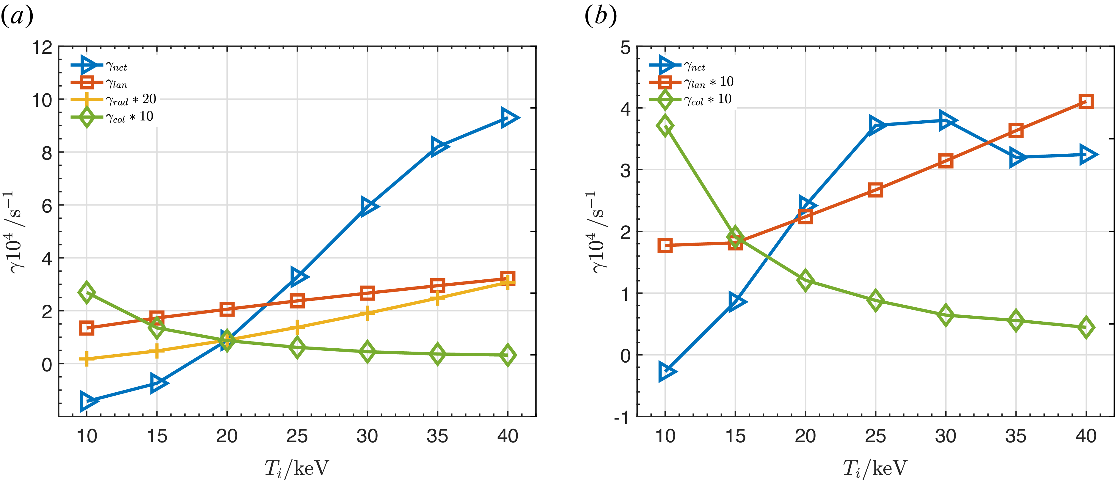
, we show the absolute values of drive and damping rates in figure 7. It is observed that the background ion temperature significantly affects the instability when the self-consistent variations in alpha particle density and beta are considered. Overall, the drive intensity grows continuously with temperature, although the rate of drive increase gradually diminishes, primarily due to the contribution of passing particles. An evident reason for this is that as
 $T_i$
rises,
 $n_\alpha$
increase accordingly, and the substantially elevated alpha particle beta significantly enhances the drive strength. However, as
 $v_A$
is approaching the alpha particle birth velocity (
 $v_{\alpha 0}=1.3\times 10^7\,\mathrm{m\,s}^{-1}$
), the drive is weakened and becomes saturated. Higher frequencies for odd TAEs induce an earlier saturation since the drive from passing particles decreases when the resonant velocity is comparable with
 $v_{\alpha 0}$
.
Growth and damping rates varying with plasma temperature for (a) even TAEs (
 $n=5$
) and (b) odd TAEs (
 $n=6$
).

Figure 7. Long description
Two line graphs depict growth and damping rates varying with plasma temperature for even and odd TAEs. Panel A: The line graph shows the growth and damping rates for even TAEs. The horizontal axis represents plasma temperature (T_i) in keV, ranging from 10 to 40 keV. The vertical axis represents the growth and damping rates (gamma) in units of 10^4 per second. The graph includes four data series: gamma_net (blue triangles), gamma_lan (orange squares), gamma_rad multiplied by 20 (yellow crosses), and gamma_col multiplied by 10 (green diamonds). The gamma_net series shows an increasing trend with temperature, while the other series exhibit varying trends. Panel B: The line graph shows the growth and damping rates for odd TAEs. The horizontal axis represents plasma temperature (T_i) in keV, ranging from 10 to 40 keV. The vertical axis represents the growth and damping rates (gamma) in units of 10^4 per second. The graph includes three data series: gamma_net (blue triangles), gamma_lan multiplied by 10 (orange squares), and gamma_col multiplied by 10 (green diamonds). The gamma_net series shows a fluctuating trend, while the gamma_lan series shows a decreasing trend and the gamma_col series shows a relatively stable trend.
From the dampings shown in figure 7, it is observed that the background ion Landau damping increases with the background temperature and is the major damping mechanism. Although the background ion beta and the velocity ratio
 $v_A/v_{ti}$
remain constants, resulting in a nearly invariant normalised Landau damping rate, the absolute damping value increases with the increasing
 $\omega _A$
:
 $\gamma _{lan} \propto \sqrt {T_i}$
. The increase in radiative damping is even more pronounced. The parameter
 $\eta _m$
in (3.6) is proportional to the ion gyroradius and thus directly proportional to the temperature. Given that the absolute damping rate is also proportional to the mode frequency, these two factors combine to cause a substantial increase in radiative damping as the temperature rises.
3.3. Dependence of magnetic field strength
The magnetic field strength
 $B$
is another key parameter in tokamaks, as higher magnetic fields are conducive to enhance the plasma confinement. With the continuous advancements of high-temperature superconducting technology, achievable magnetic field strength has significantly increased. To explicitly determine the relationship between the fusion triple product
 $n\tau _ET$
and parameters such as background temperature, density, device size and magnetic field strength, we refer to the dimensionless H-mode confinement time scaling law from Luce, Petty & Cordey (Reference Luce, Petty and Cordey2008):
 \begin{align} \varOmega _i\tau _E\propto \rho _*^{-3.15}\beta ^{-0.01}\nu _c^{-0.35}q_{95}^{-1.43}\kappa ^{2.2}, \end{align}
where the terms are defined as follows: the ion cyclotron frequency
 $\varOmega _i=e_iB/m_i$
; the normalised ion Larmor radius
 $\rho _*\equiv \sqrt {T_im_i}/(e_iB a)$
; the background plasma beta
 $\beta$
; the collisionality normalised to the thermal transit frequency
 $\nu _c\propto n_eR/T_e^2$
; the safety factor
 $q_{95}$
and the elongation
 $\kappa$
. In this expression, the energy confinement time
 $\tau _E$
refers specifically to the thermal plasma energy and excludes the contribution from EPs. Under the constraints of maintaining a constant plasma beta and a fixed triple product
 $n\tau _ET$
, variations in the magnetic field strength will inevitably induce changes in other parameters.
The major radius
 $R_0$
, minor radius
 $a$
, background plasma temperatures and densities are assumed to be varied with
 $B$
, while the aspect ratio
 $\epsilon$
and bulk beta
 $\beta _b$
remain invariant. The physical rationale is that increasing the magnetic field strength allows for a strategic reduction in device size to develop compact devices for economic efficiency without compromising confinement performance. Maintaining a constant plasma beta implies
 $nT \propto B^2$
. Disregarding the Greenwald density limit, we select the scaling
 $n \propto B$
and
 $T \propto B$
. Keeping the safety factor and elongation constant, the scaling law can be transformed accordingly:
 \begin{align} B\tau _E&\propto \big(B^{-0.5}a^{-1}\big)^{-3.15}(RB^{-1})^{-0.35} \nonumber\\[3pt] &\propto B^{1.925}\epsilon ^{3.15}R^{2.8}, \nonumber\\[3pt] n\tau _ET &\propto B^{2.925}R^{2.8}. \end{align}
It means that
 $a,R\propto B^{-1.05}$
. Based on this premise, we analyse the impact of magnetic field strength on mode stability within the range of
 $3 \sim 8\,\mathrm{T}$
.
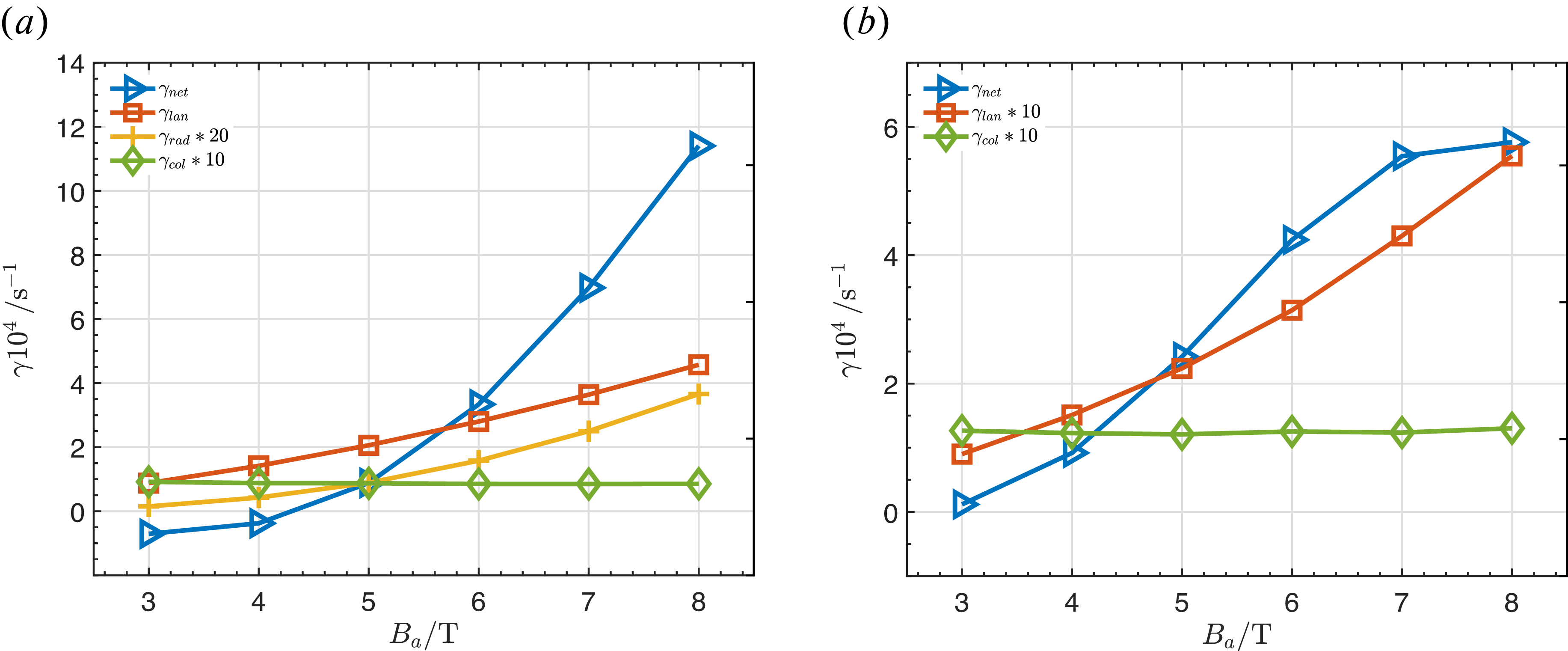
Growth and damping rates varying with magnetic field strength for (a) even TAEs (
 $n=5$
) and (b) odd TAEs (
 $n=6$
).

We find that the mode structures and normalised mode frequencies remain unchanged at a fixed plasma beta. This is because (2.1) involves the
 $\varDelta ^{\prime }$
term, which remains constant due to the invariant aspect ratio
 $\epsilon$
. Since both background ion temperature and density increase linearly with
 $B$
, the alpha particle density formula yields
 $n_\alpha \propto n_iT_i^{7/2}\propto B^{9/2}$
. Neglecting minor variations in
 $T_\alpha$
, we obtain
 $\beta _\alpha \propto B^{5/2}$
. Same as the above-mentioned cases, the saturations of EP drive result from the increasing resonant velocity shown in figure 8 (even TAEs will saturate with higher
 $B$
). Radiative damping increases with the magnetic field strength because the parameter
 $\eta _m$
in (3.6) scales as
 $\eta _m\propto B^{-1}a^{-2}\propto B^{1.09}$
under self-consistent size variations. Meanwhile, the absolute Landau damping rate increases approximately as
 $\gamma _{lan}\propto B^{1.55}$
due to the increasing Alfvén frequency.
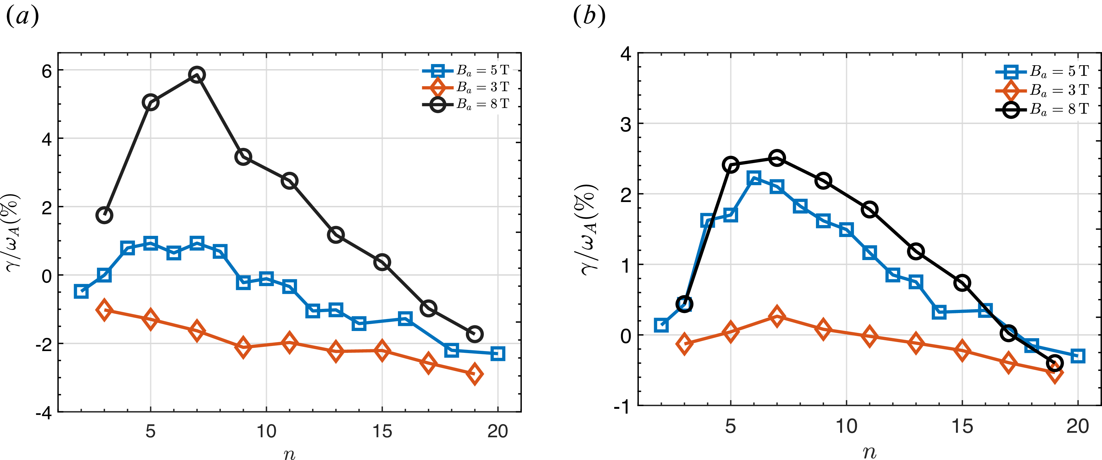
Impact of magnetic field on instabilities with different mode numbers for (a) even TAEs and (b) odd TAEs.

We analyse the impact of magnetic field strength on the most unstable core-localised TAE. Figure 9 shows the net growth rates for different toroidal mode numbers at three
 $B_a$
values. The results indicate that while maintaining a fixed fusion triple product, the instability growth rate increases significantly with
 $B$
due to the substantially higher alpha particle beta, while the odd TAEs have a smaller increase because of the larger increase of Landau damping at
 $B=8\,\mathrm{T}$
. The shift in the most unstable toroidal mode number is relatively small. This is because the most unstable
 $n$
is approximated by
 $k_\perp \rho _h\sim 1$
, which leads to
 $k_\perp \rho _h\approx ({m}/{r})\rho _h\propto B^{0.55}$
. In summary, while magnetic field variations do not alter the mode structures, EP drives increase with the significantly elevated
 $\beta _\alpha$
under self-consistent parameter variations. Radiative damping increases due to the
 $\eta _m$
parameter and Landau damping increases with the absolute Alfvén frequency, even as the
 $v_{ti}/v_A$
ratio remains constant at fixed beta.
3.4. Another variation scaling of magnetic field for even TAEs
When varying the magnetic field strength, multiple options exist for the self-consistent evolution of other parameters. Here, we consider an alternative variation: maintaining the plasma temperature, the safety factor and aspect ratio constant while varying the device size and background density. Considering the Greenwald density limit and assuming a constant density ratio
 $n/n_{GW}$
, it follows that
 $n\propto ({I}/{a^2})\propto ({Ba}/{a^2})\propto ({B}/{a})$
. By substituting this back into the scaling law (3.7), we have
 \begin{align} B\tau _E& \propto B^{3.15}a^{3.15}(nB^{-2})^{-0.01}(nR)^{-0.35} \nonumber\\ & \propto B^{3.17}\epsilon ^{3.15}R^{2.8}n^{-0.36}, \nonumber\\ n\tau _ET& \propto B^{2.17}R^{2.8}n^{0.64} \nonumber\\ & \propto B^{2.81}R^{2.16}. \end{align}
By maintaining a constant fusion triple product, we obtain
 $a,R\propto B^{-1.3}$
. Consequently, the background density scales as
 $n\propto B/a\propto B^{2.3}$
, and the relation between plasma beta and the magnetic field becomes
 $\beta \propto n/B^2\propto B^{0.3}$
.
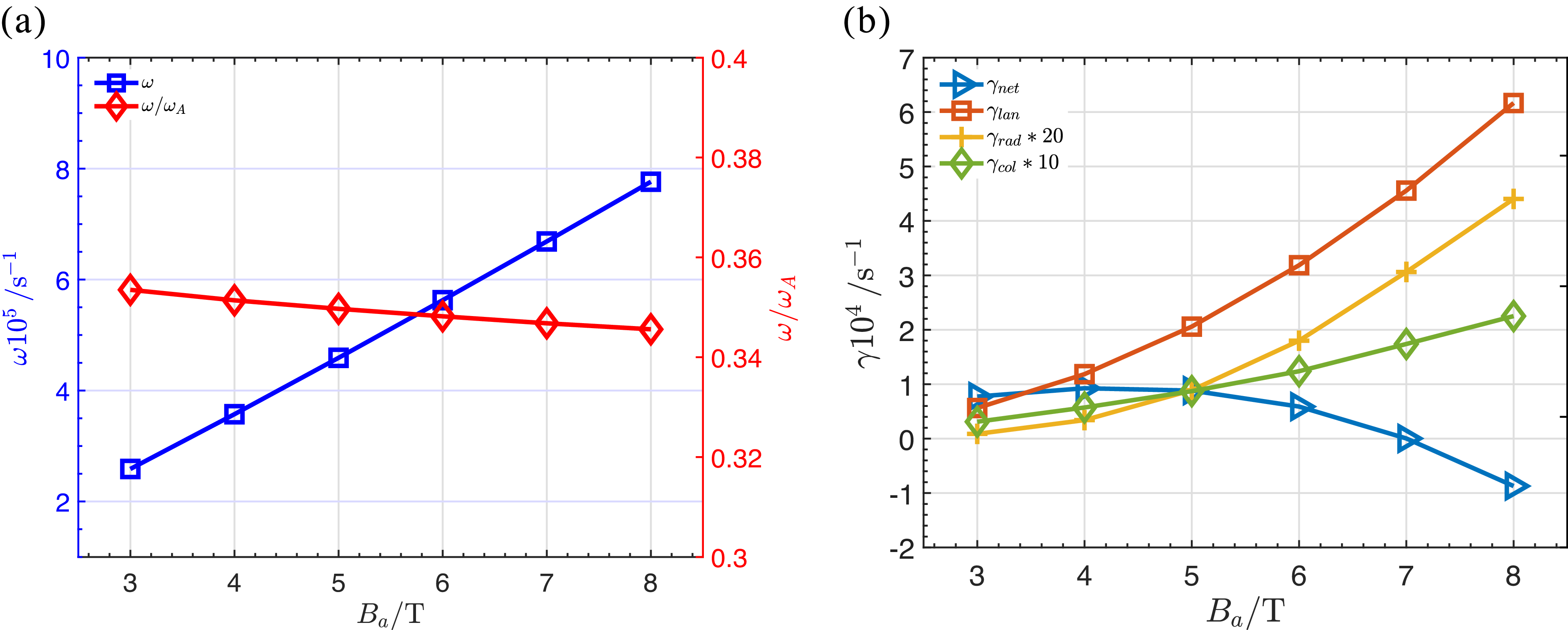
(a) Frequencies, (b) growth rates and dampings varying with magnetic field in a different way for even TAE (
 $n=5$
).

When performing a parameter scan of the magnetic field strength in this manner, the Alfvén frequency evolves as
 $\omega _A\propto B/(R\sqrt {n})\propto B^{1.15}$
. Since the background beta varies, the normalised frequency decreases with increasing magnetic field strength and background beta, shown in figure 10. The Landau damping induced by background ions varies significantly with background beta. For core-localised TAEs, the normalised Landau damping is approximately proportional to the background beta as
 $\gamma _{lan} \propto \beta _b \exp (-\lambda \beta _b^{-1})$
with
 $\lambda$
being a constant and related with the TAE resonant parameter
 $l$
(
 $v_\parallel =\pm v_A/(2l+1)$
), which explains the sharp increase in Landau damping with magnetic field strength observed in figure 10. Given
 $n_\alpha \propto n_i\propto B^{2.3}$
and
 $\beta _\alpha \propto B^{0.3}$
, the alpha particle drive is initially proportional to
 $B^{0.3}$
. However, as the parameter
 $v_A/v_{\alpha ,0} \propto B^{1.15}$
increases, the drive further increases within a certain range, albeit with a diminishing slope. The relation between the overall net growth rate and the magnetic field strength can be expressed as
 $\gamma _{net}\propto ({f_1(B)}/{(f_2(B)\exp (-B^{-0.3}))})$
, where
 $f_1(B)$
and
 $f_2(B)$
are polynomial functions of
 $B$
. This value decreases with the sustained increase of magnetic field. Accordingly, the alpha particle beta threshold shifts from
 $0.41\,\% (3\,\mathrm{T})\to 0.74\,\%(5\,\mathrm{T})\to 1.47\,\%(8\,\mathrm{T})$
. This is a positive trend for high field devices.
3.5. Summary and comparison
Analytic investigations of linear stability of core-localised TAEs with a simplified model have been carried out in this section. The ion temperature and magnetic field as two key parameters in tokamaks with specific variation patterns are considered, for instance, while other parameters and other variation patterns can be also studied by the same procedure. This simplified model offers a qualitative understanding about the parameter dependences of TAEs. This model can be extended to investigate the linear stability of beta-induced Alfén eigenmodes and reversed shear Alfén eigenmodes as well.
Now, we discuss the differences between even and odd core-localised TAEs. With increases of absolute frequencies along with the increases of
 $T_i$
and
 $B$
, contribution of the
 $v_A/3$
resonance is gradually increasing and becomes comparable with the
 $v_A$
resonance for odd TAEs, while the
 $v_A$
resonance is the only dominant drive for even TAEs. Additionally, in contrast to the single dominant
 $v_A/3$
resonance in the even TAE cases, the ion Landau damping of odd TAEs arises from the combined contributions of
 $v_A/3$
and
 $v_A/5$
resonances. Core-localised TAEs, including even and odd TAEs, have the same tendencies with respect to the key parameter dependences, while the different mode structures and frequencies result in quantitative differences of the absolute drive and damping values.
4. Linear stability of global TAEs in ITER
In this section, we shift our focus to the linear stability of global TAEs. For this purpose, the
 $q$
-profile is adopted from the blue dashed line in figure 3 and
 $\beta _b=6.4\,\%$
is the original value, while all other parameters and profiles remain consistent with those used in the previous section. Equation (2.1) is still employed to solve the individual poloidal harmonics
 $\delta \varPhi _m$
of the TAE. However, to account for the coupling among multiple
 $m$
harmonics, it is necessary to simultaneously incorporate the
 $m-1$
and
 $m+1$
coupling terms into the governing equation for each
 $m$
. Since the equilibrium quantities in the coupled equation are evaluated at the peak of mode amplitude
 $r_m$
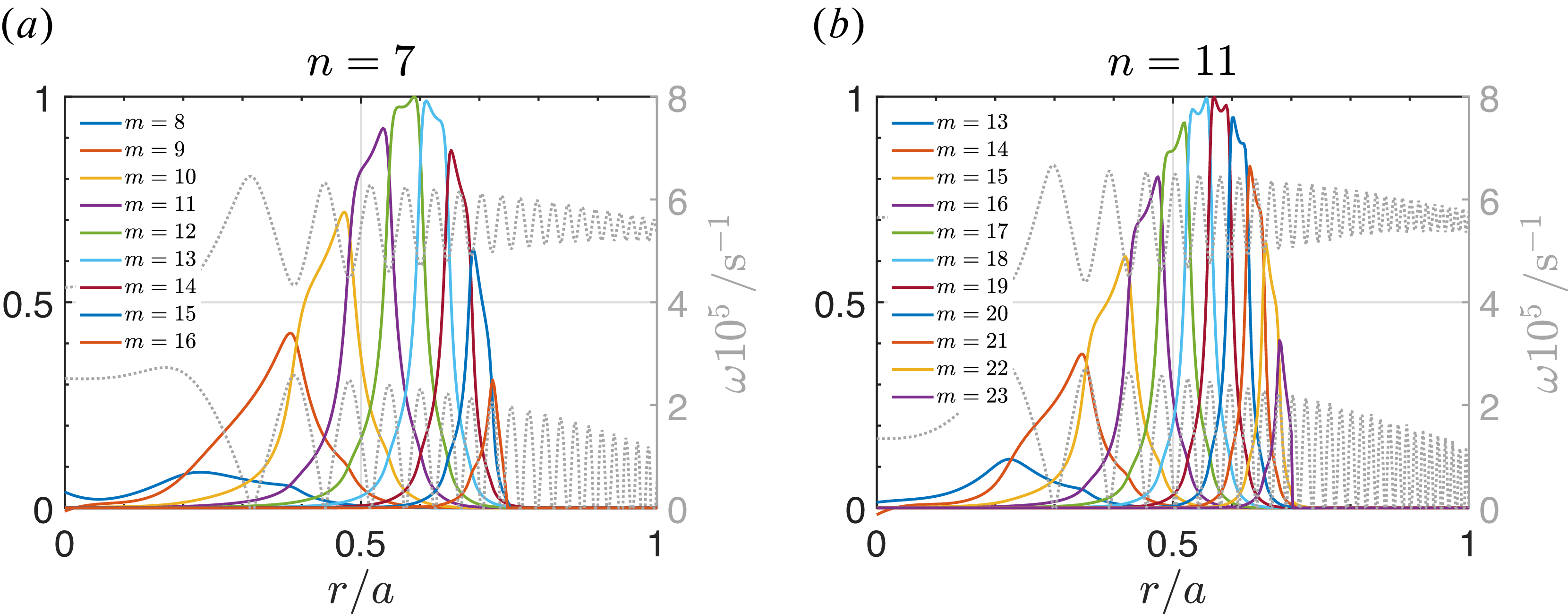
, this model does not strictly apply to other poloidal harmonics coupled at different radial positions. Therefore, the current multi-mode coupling approach is treated as a numerical approximation. Figure 11 presents the one-dimensional radial mode structures for two typical toroidal mode numbers. Furthermore, as
 $n$
increases, each poloidal component of the global TAE becomes progressively narrower, leading to a gradual localisation of the overall mode structure.
Global TAEs with mode number
 $n=$
(a) 7 and (b) 11.

Figure 11. Long description
Two line graphs depict the relationship between normalized radius and frequency for different mode numbers. Panel A: The line graph shows the frequency (omega) in units of 10^5 s^-1 versus the normalized radius (r/a) for mode number n = 7. The lines represent different mode numbers (m) ranging from 8 to 16. The frequency peaks at different normalized radii for each mode number. Panel B: The line graph shows the frequency (omega) in units of 10^5 s^-1 versus the normalized radius (r/a) for mode number n = 11. The lines represent different mode numbers (m) ranging from 13 to 23. Similar to Panel A, the frequency peaks at different normalized radii for each mode number.
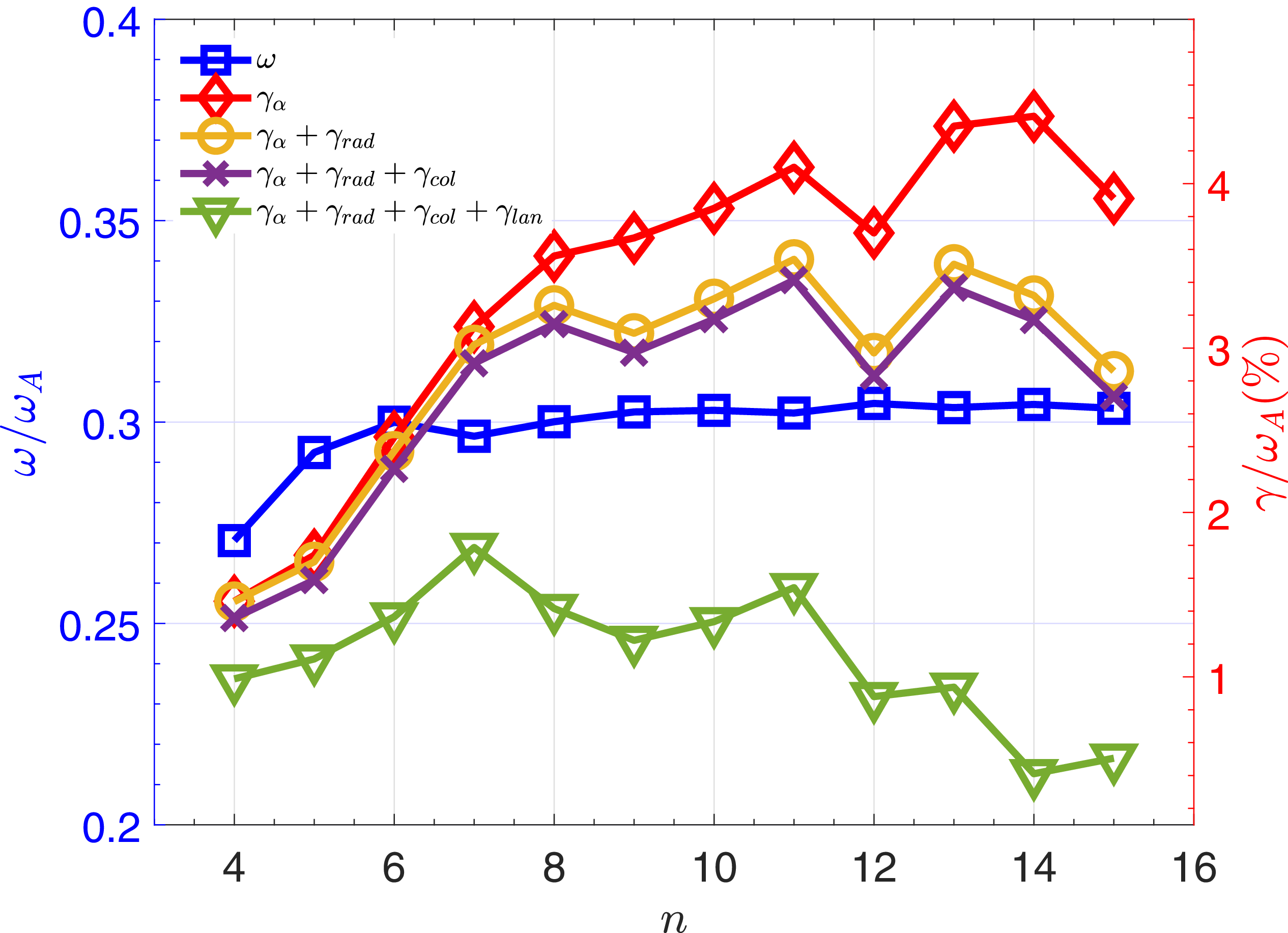
Growth rates and frequencies varing with
 $n$
for global TAEs.

Following the same procedure used in the core-localised TAE calculations, we first present the dependence of the global TAE growth and damping rates on the toroidal mode number (figure 12). The radiative damping rate calculated here corresponds to the relative position of the mode eigenfrequency within the local gap formed by
 $m$
and
 $m+1$
, without explicitly accounting for global effects. Unlike the core-localised TAE cases,
 $h_m$
in the expression uses the continuum boundaries calculated from the multi-
 $m$
coupling form of (2.2); consequently, the continuum matrix must be also updated to its multi-
 $m$
coupling representation. In practice, we adopt the upper and lower boundary values of the continuum gap at the location of the peak of mode structures. As illustrated in figure 12, the most unstable mode is
 $n=7$
and, therefore, the beta threshold is
 $\beta _{\alpha ,c}\approx 0.79\,\%$
. The global TAEs are unstable across all investigated mode numbers, which is attributed to the higher prescribed alpha particle beta. It is found that the radiative damping for all toroidal mode numbers are larger than those of the localised TAEs. This is because the parameter
 $\eta _m$
is proportional to the magnetic shear
 $s$
; thus, the large magnetic shear required for the coupling of multiple poloidal harmonics also leads to a significantly enhanced radiative damping rate.
4.1. Dependences of parameters
Similarly, we perform a parameter scan of the background ion temperature for the global TAEs. In this analysis, the alpha particle density and beta are derived self-consistently from the aforementioned formulae. Consistent with the localised TAE results, the ion temperature does not affect the mode structures or the normalised frequencies
 $\omega /\omega _A$
. The absolute frequency varies with
 $\sqrt {T_i}$
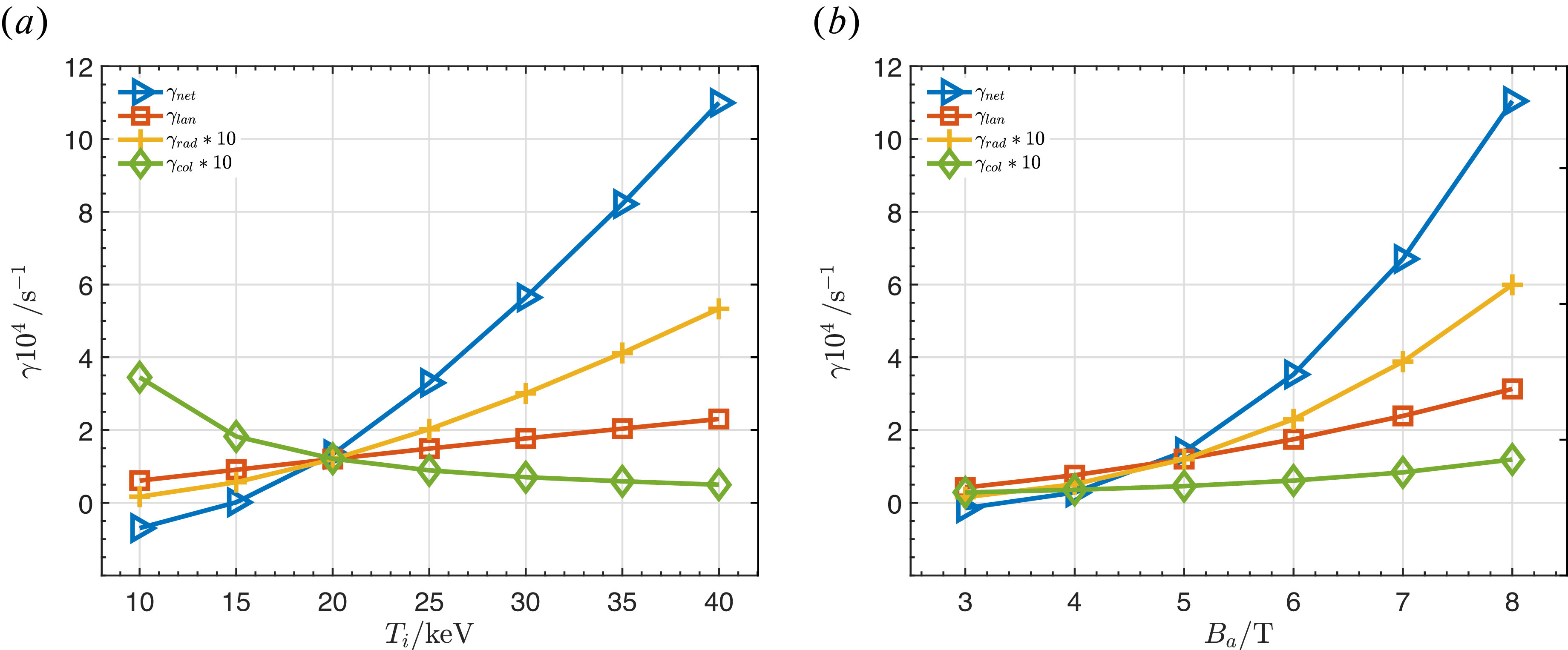
. Figure 13(a) illustrates the dependences of the alpha particle drive and background damping rates on the ion temperature. Due to the strong correlation between alpha particle beta and the background ion temperature, the EP drive exhibits significant variation. In contrast to the results of core-localised TAE, the global TAE drive shows no signs of saturation within the temperature range. This is attributed to the higher background particle density in the global case: as the background temperature increases, the alpha particle density and beta grow more rapidly and remain less affected by saturation factors. Furthermore, the instability temperature threshold for the global TAEs is approximately
 $T_{i,c}\sim 15\,\mathrm{keV}$
, which is lower than the
 $T_{i,c}\sim 18\,\mathrm{keV}$
observed in core-localised TAE cases. This discrepancy is primarily because the core-localised TAEs are located closer to the plasma core, where the background beta is slightly higher than that of global TAEs, leading to stronger background Landau damping. In fact, with the same alpha particle beta, the global TAEs exhibit both lower alpha particle drive and lower ion Landau damping compared with the core-localised TAEs, due to their more outward radial positions. As previously discussed, the parameter
 $\eta _m$
in the radiative damping expression is proportional to the temperature, causing the damping rate to increase with
 $T_i$
. Moreover, due to the higher magnetic shear associated with these parameters, the radiative damping for the global TAEs are several times larger than those of core-localised TAEs.
Global TAEs with (a)
 $T_i$
and (b)
 $B_a$
dependences for
 $n=7$
.

Figure 13. Long description
Two line graphs depict the dependences of global TAEs. Panel A: The line graph shows the growth rate (gamma) in units of 10^4 per second on the vertical axis against the ion temperature (Ti) in keV on the horizontal axis. The graph includes four data series: net growth rate (gamma_net) represented by blue triangles, lan growth rate (gamma_lan) represented by orange squares, rad growth rate (gamma_rad) multiplied by 10 represented by yellow crosses, and col growth rate (gamma_col) multiplied by 10 represented by green diamonds. The net growth rate increases significantly with higher ion temperatures, while the other rates show varying trends. Panel B: The line graph shows the growth rate (gamma) in units of 10^4 per second on the vertical axis against the magnetic field strength (Ba) in tesla on the horizontal axis. Similar to Panel A, it includes the same four data series with the same symbols. The net growth rate again increases with higher magnetic field strengths, with the other rates showing different patterns.
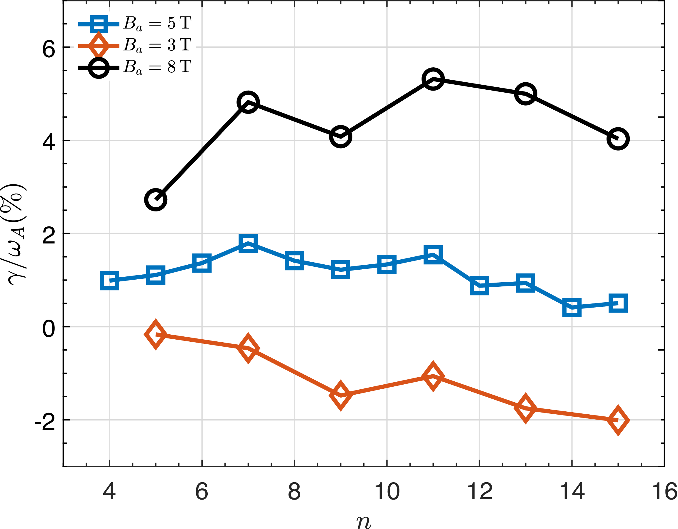
The results of the self-consistent parameter scan with incorporating variations in magnetic field, device size, background ion temperature and density based on the scaling law (3.6) are presented in figure 13(b). The findings for global TAEs are qualitatively consistent with those obtained for the core-localised TAEs. Furthermore, the toroidal mode number scans performed for the two magnetic field values,
 $B_a=3\,\mathrm{T}$
and
 $B_a=8\,\mathrm{T}$
, also yield results that align qualitatively with the core-localised TAE cases. It is observed that as the magnetic field strength varies, the shift in the most unstable toroidal mode number is relatively small compared with the substantial changes in the growth rates (see figure 14).
Impact of magnetic field on instabilities with different mode numbers for global TAEs.

5. Summary and discussion
Based on the ITER baseline scenario, we calculate the mode structures, the drive and damping rates for core-localised TAEs with low magnetic shear
 $q$
-profile and global TAEs with higher magnetic shear
 $q$
-profile under a circular cross-section approximation. Distinct from the global TAEs, the frequencies of the core-localised TAEs shift downward as the background plasma beta increases, eventually merging into the Alfvén continua and becoming stabilised by strong continuum damping. Therefore, to theoretically obtain clear and observable core-localised TAE structures, we reduce the background beta in our study. While the background beta in this simplified circular configuration exceeds the existence threshold for core-localised even TAEs, the same beta value might not surpass the threshold in realistic magnetic configurations. Through a scan of toroidal mode numbers, we find that the most unstable
 $n$
for core-localised TAEs is smaller than that for global TAEs, as the former is located closer to the plasma core. They have nearly the same alpha beta threshold around
 $1.0\,\%$
.
About the most unstable mode numbers, we have smaller values than that of Rodrigues et al. (Reference Rodrigues, Figueiredo, Ferreira, Coelho, Nabais, Borba, Loureiro, Oliver and Sharapov2015). The deviation could come from the several reasons as explained as follows. First, the circular flux surfaces approximation. The realistic D-shaped geometry results in a larger effective radius because of the elongation, which will lead to larger unstable mode numbers. Second, the FLR effect. No FLR effects were included in Rodrigues’s results and the introduced FLR effect tends to suppress the high-
 $n$
modes. Third, the q-profile. We adopt the q-profile with larger magnetic shear while the flatter q-profile and weaker magnetic shear used in Rodrigues’s paper is more beneficial for the growth of high-
 $n$
modes. Fourth, the locations for core-localised TAEs (
 $r/a\approx 0.28$
) have smaller radiuses as compared with Rodrigues’s (
 $r/a\approx 0.4$
), which corresponds to lower
 $n$
of the most unstable modes. In addition, they have more accurate methods to calculate the mode structures, which will also affect the drive and dampings, and therefore, the most unstable mode numbers. As for the results from Hayward-Schneider et al. (Reference Hayward-Schneider, Lauber, Bottino and Lu2021, Reference Hayward-Schneider, Lauber, Bottino and Mishchenko2022), except for the reasons listed previously (FLR effects were included in Hayward-Schneider’s paper), we have chosen the simplified physical model which is significantly different from their gyrokinetic model. Back to our analytical results, we emphasise more on the qualitative dependences of the linear stability of TAEs on key parameters.
In our simplified theoretical model, the radiative damping and trapped electron collisional damping of TAEs are much smaller than the Landau damping mainly caused by the background ion
 $v_\parallel =\pm v_A/3$
resonance. Due to the higher magnetic shear, global TAEs experience stronger radiative damping; furthermore, higher-
 $n$
modes exhibit increasing damping rates due to the scaling
 $\eta _m\propto n^2$
. Collisional damping is closely related to the bulk density and temperature: it becomes comparable to the radiative damping for lower temperatures and higher densities. Global TAEs experience higher collisional damping than core-localised TAEs for higher bulk density. For core-localised TAEs, the continuum varies smoothly near the gap and the mode width is narrow, rendering continuum damping negligible. Even though the global TAEs are with wider mode structures, the descending continuum of this ITER baseline scenario avoids the intersection between the mode and the continuum in the edge, thus the continuum damping is also negligible. However, the continuum damping, especially for global TAEs, should be included when considering realistic density profiles instead of constant densities chosen here. For the modes with
 $n\gg 1$
, there are well-known analytical formulations for continuum damping valid in this limit (Rosenbluth et al. Reference Rosenbluth, Berk, Dam and Lindberg1992; Zonca & Chen Reference Zonca and Chen1992), which can be treated in the same way as radiative damping presented before. Therefore, the global TAEs with relatively low
 $n$
values would be more stable than the core-localised TAEs and higher-
 $n$
global TAEs.
It should be noted that the current study employs a circular cross-section approximation, and the mode structures and instability thresholds may vary in realistic magnetic geometries. Additionally, the treatment of radiative damping for global TAEs is an approximation that only considers the
 $m$
and
 $m+1$
coupling at the maximum amplitude location, which may lead to an underestimation of the damping rate. Furthermore, we consider the perturbative contributions from EPs to the mode growth rate and structures of TAE instabilities, which would be not appropriate under high EP beta and underestimate the kinetic effects from EPs.
Regarding the parameter scans, we analyse the variations in mode drive and dampings under self-consistent changes in background ion temperature and magnetic field strength. When maintaining a constant plasma beta or fusion triple product
 $n\tau _ET$
, the device size, background density and temperature vary accordingly. The alpha particle density and beta, which is calculated self-consistently from the fusion reaction rate and slowing-down time formulae, also undergo corresponding changes. These factors do not alter the mode structure or the normalised frequency, but the resulting variations in alpha particle beta and Alfvén velocity significantly affect the alpha particle drive and background dampings. With increases of bulk particle temperature and magnetic field strength, the corresponding increases of alpha density and beta originating from the increasing fusion rate result in enhancement of TAE instabilities and finally the saturation. The tendency along magnetic field is consistent with the results of Tolman et al. (Reference Tolman, Loureiro, Rodrigues, Hughes and Marmar2019) in which theoretical and numerical methods are both used. However, if we allow the variations of plasma beta which significantly influence the bulk ion Landau damping, the increase of magnetic field induces the stabilisation of TAEs. Indeed, the parameter variation patterns significantly impact the linear stability of TAEs and we can employ our workflow to investigate these instabilities under various scans of parameters.
Compared with the previous study on the linear stability of TAEs in burning plasmas by Gorelenkov et al. (Reference Gorelenkov, Berk, Budny, Cheng, Fu, Heidbrink, Kramer, Meade and Nazikian2003), our work focuses on different types of TAEs and conducts systematic linear stability analyses of their parameter dependences under different variations. A more accurate treatment for the ion Landau damping, and analytical radiative damping and trapped electron collisional formulae are employed in our work. Regarding the trend analyses, both studies demonstrate an increasing drive associated with rising bulk temperatures under consistent alpha particle calculation. Furthermore, the systematic assessment by Rodrigues et al. (Reference Rodrigues, Figueiredo, Ferreira, Coelho, Nabais, Borba, Loureiro, Oliver and Sharapov2015) encompasses all AEs across a broad range of frequencies and mode numbers under ITER-like equilibria, highlighting the destabilisation of core-localised TAEs in low magnetic shear regions.
Acknowlegements
The first author appreciates useful and instructive discussions with Mr. Qi Zhong.
Editor Tünde Fülöp thanks the referees for their advice in evaluating this article.
Funding
This work was supported by the National Key R&D Program of China (Grant NO. 2019YFE03050001), the National Natural Science Foundation of China (Grant No. 11875235).
Declaration of interests
The authors report no conflict of interest.

 n=6
 n=(a)
 n=(a)
 n
 n=5
 n=6
 n=5
 n=6
 n=5
 n=
 n
 Ti
 Ba
 n=7

 Open access

