1. Introduction
Turbulence and magnetic reconnection are key fundamental nonlinear processes in weakly collisional plasmas governing energy conversion and transport. Astrophysical plasmas, such as solar winds, accretion discs, the interstellar medium, as well as fusion plasmas are mostly collisionless and in a turbulent state (Biskamp Reference Biskamp2003). Plasmas tend to form current sheets where magnetic reconnection occurs to release the magnetic energy and convert it into heat (Biskamp Reference Biskamp2000). Turbulence and magnetic reconnection often coincide. Solar winds are the most typical examples of such a situation (e.g. Retinò et al. Reference Retinò, Sundkvist, Vaivads, Mozer, André and Owen2007) and provide rich observational information about these processes.
According to the conventional wisdom of turbulence (see e.g. Frisch (Reference Frisch1995) for neutral fluids and Biskamp (Reference Biskamp2003) for plasmas), turbulent fluctuations are known to possess universality properties. In homogeneous turbulence driven at a large scale by an external forcing or instability, the injected energy at  $k_{\mathrm {in}}^{-1}$ cascades down to smaller scales via local interactions at a constant energy transfer rate, and is eventually dissipated at small scales
 $k_{{d}}^{-1}$ by some dissipation mechanisms. In neutral fluid turbulence, the viscosity (
 $\mu$) sets the dissipation scale such that the dissipation (
 $\propto \mu k_{{d}}^{2}$) balances with the energy injection power. In the inertial range
 $k_{\mathrm {in}} \ll k \ll k_{{d}}$, the wavenumber spectrum of the kinetic energy follows the well-known Kolmogorov spectrum
 $k^{-5/3}$.
Unlike rather simple neutral fluid turbulence, plasma turbulence is complex because it consists of multiple species (most simply, electrons and single-species ions), is anisotropic, and has several linear wave modes. There are numerous energy flow channels in plasmas, and it is generally unknown which path the energy takes and what mechanisms effectively work to dissipate the energy. Possible paths of cascades and dissipation mechanisms in magnetized plasma turbulence are described comprehensively in Schekochihin et al. (Reference Schekochihin, Cowley, Dorland, Hammett, Howes, Quataert and Tatsuno2009). In plasmas, the energy carried by Alfvén waves and compressive modes reaches the ion kinetic scale  $k\rho _{{i}}\sim 1$ (if collisions are rare) where kinetic effects start to play roles: phase space of cascades is extended into velocity space. Kinetic effects generally lead to non-Maxwellian distribution functions, i.e. structures in velocity space are generated, which suffer strong collisional dissipation as the collision operator provides diffusion in velocity space. Landau damping along the mean magnetic field and perpendicular phase mixing owing to finite Larmor radius effects are examples of dissipation mechanisms in kinetic plasmas.Footnote 1
Recently, high-performance kinetic simulations and hybrid fluid-kinetic modelling covering a wide range of dynamical scales have become feasible (Grošelj et al. Reference Grošelj, Cerri, Navarro, Willmott, Told, Loureiro, Califano and Jenko2017), and increasing numbers of numerical studies have been devoted to the study of dissipation in kinetic turbulence. Full gyrokinetic simulations were carried out to study electromagnetic turbulence at the sub-ion Larmor regime aimed at explaining the energy spectra observed in solar winds. The competition of the ion entropy cascade resulting in ion heating and kinetic Alfvén wave cascade which carries part of the energy into electron heat was demonstrated (Howes et al. Reference Howes, TenBarge, Dorland, Quataert, Schekochihin, Numata and Tatsuno2011; Told et al. Reference Told, Jenko, TenBarge, Howes and Hammett2015). Thermal energy partition in wide parameter space was explored using a hybrid model for applications to accretion flows (Kawazura, Barnes & Schekochihin Reference Kawazura, Barnes and Schekochihin2019). In the absence of the kinetic Alfvén waves, the ion entropy cascade primarily works as the ion dissipation mechanisms via nonlinear phase mixing in the plane perpendicular to the mean field. The electrostatic plasma turbulence in two dimensions and the nonlinear phase mixing were studied theoretically (Plunk et al. Reference Plunk, Cowley, Schekochihin and Tatsuno2010) and numerically (Tatsuno et al. Reference Tatsuno, Dorland, Schekochihin, Plunk, Barnes, Cowley and Howes2009, Reference Tatsuno, Barnes, Cowley, Dorland, Howes, Numata, Plunk and Schekochihin2010, Reference Tatsuno, Plunk, Barnes, Dorland, Howes and Numata2012). Compressive fluctuations in Alfvénic turbulence were found to have fluid-like spectra because the phase mixing is strongly suppressed. The fluidisation is considered as a reason for the observed scalings in solar winds (Schekochihin et al. Reference Schekochihin, Parker, Highcock, Dellar, Dorland and Hammett2016; Meyrand et al. Reference Meyrand, Kanekar, Dorland and Schekochihin2019), which is shallower compared with the scaling obtained from a kinetic treatment.
Magnetic reconnection in weakly collisional environments also works as a process of plasma heating via phase mixing. In addition to the electron heating due to parallel phase mixing in low- $\beta$ plasmas (Loureiro, Schekochihin & Zocco Reference Loureiro, Schekochihin and Zocco2013; Numata & Loureiro Reference Numata and Loureiro2014) (
 $\beta$ is the ratio of plasma pressure and magnetic pressure), it is shown that the nonlinear phase mixing becomes a significant ion-heating mechanism in high-
 $\beta$ plasmas during reconnection (Numata & Loureiro Reference Numata and Loureiro2015). In the existence of magnetic field structures, such as the reconnection magnetic field, the assumption of local interaction no longer holds. By creating structures, plasmas may dynamically change the energy flow channel, thus further complicating the dissipation process.
This work is primarily motivated by the challenge to understand how plasmas convert the macroscopic energy into heat during turbulent magnetic reconnection in weakly collisional environments. To study this problem, we develop a method to impose external turbulence in gyrokinetic magnetic reconnection simulation using AstroGK code (Numata et al. Reference Numata, Howes, Tatsuno, Barnes and Dorland2010) to extend our previous studies (Numata & Loureiro Reference Numata and Loureiro2014, Reference Numata and Loureiro2015). We restrict our consideration to two dimensions for the sake of simplicity.
Driving turbulence in kinetic models is not straightforward as it does not directly evolve a macroscopic flow field. In the Vlasov–Maxwell equations or gyrokinetic-Maxwell equations, a distribution function coupled with electromagnetic fields via Maxwell's equations is advanced according to the Vlasov or gyrokinetic equation, and the macroscopic flow is determined by taking the velocity moment of the distribution function. A method for driving Alfvénic turbulence by injecting an external current in Ampère's law has already been developed in AstroGK code (TenBarge et al. Reference TenBarge, Howes, Dorland and Hammett2014). However, it is not suitable for studying the magnetic reconnection problem because the external current may have a significant direct effect on reconnection dynamics. Instead, we newly develop a method to directly drive flows in the gyrokinetic equation by adding a term that only pushes specific moments of a distribution function. In the gyrokinetic model, excited density fluctuations that are the zeroth-order moment of the distribution function couple with the electrostatic potential perturbations through the quasi-neutrality condition, and yield the so-called  $\boldsymbol {E}\times \boldsymbol {B}$ flows. We note that this forcing method is irrespective of the magnetic field perturbations in the plane perpendicular to the mean magnetic field and has close correspondence with forcing in two-dimensional reduced MHD equations. Kawazura et al. (Reference Kawazura, Schekochihin, Barnes, TenBarge, Tong, Klein and Dorland2020) have also implemented a similar method for exciting slow mode fluctuations by driving the parallel flow component of the distribution function in AstroGK with the isothermal electron model. This method also drives the parallel current, and is not appropriate for the magnetic reconnection study.
We also demand the forcing method to have a property that it injects energy into the system at a constant rate, thus enabling the measurement of how much of the injected energy goes into specific channels in a steady state. A method to control the injection power was proposed for neutral fluid turbulence (Alvelius Reference Alvelius1999). In the proposed method, the power input is solely determined by the force–force correlation (but not by the velocity–force correlation), thus it is pre-determined. We adopt the same method in two-dimensional gyrokinetics.
In the following sections, we first describe the developed forcing method in gyrokinetics. We perform a test simulation validating that the forcing injects energy at a constant rate, and a statistically steady state is achieved where the injected power is balanced by developed dissipation. With this forcing we demonstrate that the code successfully simulates turbulence from the large-scale fluid to small-scale kinetic regimes. The theoretically predicted scaling laws in those regimes are reproduced. We summarize the paper in § 4.
2. External forcing in gyrokinetics
The paper aims to develop a random forcing method in gyrokinetics, which directly corresponds to that in a fluid model. By taking a certain limit, the gyrokinetic model (briefly summarized in appendix A) is reduced to the reduced MHD model, which describes evolutions of the vorticity ( $\omega$) and magnetic flux (
 $\psi$) in the direction of the mean magnetic field
 $\boldsymbol {B}_{0}=B_{0}\boldsymbol {z}$. In the reduced MHD, a forcing term can be written as
 \begin{equation} \frac{\partial \omega}{\partial t} = \dots + a, \end{equation}
where  $a=(\boldsymbol {\nabla }\times \boldsymbol {F})\boldsymbol {\cdot }\boldsymbol {z}$ with
 $\boldsymbol {F}$ being a force. (We omit all terms other than the forcing for simplicity. The dots indicate the omission.) In gyrokinetics, the flow perpendicular to the mean field is given by the
 $\boldsymbol {E}\times \boldsymbol {B}$ drift, therefore the vorticity becomes
 $\omega =\boldsymbol {\nabla }_{\perp }^{2}\phi /B_{0}$ (
 $\phi$ is the electrostatic potential,
 $\boldsymbol {\nabla }_{\perp }^{2}=\partial _{x}^{2}+\partial _{y}^{2}$ is the two-dimensional Laplacian). From the quasi-neutrality condition:
 \begin{equation} \sum_{s} \left(\frac{q_{s}^{2}n_{0s}}{T_{0s}} \right) \phi = \sum_{s} q_{s} \int h_{s} \,\mathrm{d} \boldsymbol{v} = \sum_{s} q_{s} \delta n_{s}, \end{equation}
we find
 \begin{equation} \frac{\partial \omega}{\partial t} = \frac{1}{B_{0}} \boldsymbol{\nabla}_{{\perp}}^{2} \frac{\partial \phi}{\partial t} = \frac{1}{B_{0}} \frac{1}{\sum_{s}(q_{s}^{2}n_{0s}/T_{0s})} \boldsymbol{\nabla}_{{\perp}}^{2} \sum_{s} q_{s} \frac{\partial \delta n_{s}}{\partial t}. \end{equation}
Note that  $\delta n_{s}$ is the density perturbation without the Boltzmann response part. Therefore, if we add a term in the gyrokinetic equation that excites density perturbations in an appropriate form, we get forcing which drives the
 $\boldsymbol {E} \times \boldsymbol {B}$ flows.
We consider an additional term (which we shall call a forcing term though it does not literally mean a force) in the gyrokinetic equation in the following form:
 \begin{gather} \frac{\partial g_{\boldsymbol{k},s}}{\partial t} = \dots + A_{\boldsymbol{k},s}, \end{gather}
 \begin{gather}A_{\boldsymbol{k},s} = f_{0s} \varXi_{\boldsymbol{k},s}(\boldsymbol{v}) \varPhi_{\boldsymbol{k}}. \end{gather}
Again, we omit all terms other than the forcing term. Here  $f_{0s}$ is a Maxwellian distribution function of a species
 $s$,
 $\varPhi _{\boldsymbol {k}}$ is related to a forcing profile in the
 $x$–
 $y$ plane,
 $a_{\boldsymbol {k}}$, as will be discussed shortly. For later convenience, we consider the equation in Fourier space. The velocity dependence (
 $\varXi$) is given similar to the Hermite polynomials
 \begin{equation} \varXi_{\boldsymbol{k},s}(\boldsymbol{v}) = \textrm{e}^{{b_{s}}/{2}} \left( \frac{N_{s}^{{f}}}{n_{0s}} + \frac{T_{s}^{{f}}}{T_{0s}} \left( \frac{v_{{\perp}}^{2}}{v_{\mathrm{th},s}^{2}} -1 + \frac{b_{s}}{2} \right) \right), \end{equation}
where  $b_{s}=(k \rho _{s})^{2}/2$,
 $k=|\boldsymbol {k}|$ and
 $N_{s}^{{f}}$,
 $T_{s}^{{f}}$ are constant coefficients. The gyrokinetic correction (the terms related to
 $b_{s}$) is included to compensate for the
 $k$ dependence of the velocity integral of
 $\varXi$. We intentionally choose no
 $v_{\parallel }$ dependence of
 $\varXi$. (Kawazura et al. (Reference Kawazura, Schekochihin, Barnes, TenBarge, Tong, Klein and Dorland2020) only included a term proportional to
 $v_{\parallel }$.) Owing to this specific choice, the forcing term does not excite
 $A_{\parallel }$ and parallel current perturbations. If
 $A_{\parallel }=0$ initially, it remains zero. Therefore, we ignore
 $A_{\parallel }$ throughout the paper.
By plugging (2.4) into the time derivatives of the field equations, we obtain the expression for the electromagnetic fields induced by the forcing term as
 \begin{gather} {{\mathsf{Y}}}_{1} \frac{\partial \phi_{\boldsymbol{k}}}{\partial t} - {{\mathsf{Y}}}_{3} \frac{\partial }{\partial t} \left(\frac{\delta B_{{\parallel},\boldsymbol{k}}}{B_{0}}\right) = \dots +\varPhi_{\boldsymbol{k}} X_{N}, \end{gather}
 \begin{gather}{{\mathsf{Y}}}_{3} \frac{\partial \phi_{\boldsymbol{k}}}{\partial t} + {{\mathsf{Y}}}_{2} \frac{\partial }{\partial t} \left(\frac{\delta B_{{\parallel},\boldsymbol{k}}}{B_{0}}\right) = \dots - \varPhi_{\boldsymbol{k}} X_{P}, \end{gather}
where we have defined the following parameters for convenience,
 \begin{gather} X_{N} = \sum_{s} q_{s} N_{s}^{{f}}, \end{gather}
 \begin{gather}X_{P} = \sum_{s} (T_{0s} N_{s}^{{f}} + n_{0s}T_{s}^{{f}}), \end{gather}
and the coefficients of the field equations,  ${{\mathsf{Y}}}_{1,2,3}$, are given in appendix A. The vorticity equation is derived by solving (2.7), (2.8) for
 $\partial \phi _{\boldsymbol {k}}/\partial t$
 \begin{equation} \frac{\partial \omega_{\boldsymbol{k}}}{\partial t} = \frac{\partial }{\partial t} \left(-\frac{k^{2}\phi_{\boldsymbol{k}}}{B_{0}}\right) = \dots + \frac{1}{B_{0}}({-}k^{2}\varPhi_{\boldsymbol{k}}) \frac{{{\mathsf{Y}}}_{2}X_{N}-{{\mathsf{Y}}}_{3}X_{P}}{{{\mathsf{Y}}}_{1}{{\mathsf{Y}}}_{2}+{{\mathsf{Y}}}_{3}^{2}}. \end{equation}
Given the desired form of forcing  $a_{\boldsymbol {k}}$, we have
 \begin{equation} \varPhi_{\boldsymbol{k}} = \frac{-a_{\boldsymbol{k}}}{k^{2}} B_{0} \frac{{{\mathsf{Y}}}_{1}{{\mathsf{Y}}}_{2}+{{\mathsf{Y}}}_{3}^{2}}{{{\mathsf{Y}}}_{2}X_{N}-{{\mathsf{Y}}}_{3}X_{P}}. \end{equation}
We specify a spatial profile of the forcing by  $a_{\boldsymbol {k}}$, and a velocity space profile by
 $N_{s}^{{f}}$ and
 $T_{s}^{{f}}$ determining how density and temperature perturbations are excited. For
 $a_{\boldsymbol {k}}$, we may borrow the forcing developed for two-dimensional neutral fluid turbulence exemplified in Carnevale (Reference Carnevale, Cannon and Shivamoggi2006).
2.1. Injected energy-like quantities
The generalized energy per unit volume is given by
 \begin{equation} \bar{W} = \sum_{s} \bar{K}_{s} + \bar{M} = \sum_{\boldsymbol{k}} \left[ \sum_{s} \int \frac{T_{0s} |\delta f_{\boldsymbol{k},s}|^{2}}{2f_{0s}} \,\mathrm{d} \boldsymbol{v} + \frac{|B_{\boldsymbol{k}}|^{2}}{2\mu_{0}} \right], \end{equation}
where the bar denotes a quantity per unit volume. We denote the particle energy by  $K_{s}$ and the magnetic energy by
 $M$. (We only consider the parallel component of the magnetic energy because the forcing term does not invoke the perpendicular component.) By taking the time derivative, we obtain
 \begin{gather} \hspace{-3.2pc}\frac{\mathrm{d} \bar{K}_{s}}{\mathrm{d} t} = \dots + T_{0s} \sum_{\boldsymbol{k}} \textrm{Re} \left(\varPhi_{\boldsymbol{k}}^{{\ast}} \left[ \int h_{\boldsymbol{k},s} \varXi_{\boldsymbol{k},s} \,\mathrm{d} \boldsymbol{v} - \frac{1}{T_{0s}} \frac{{{\mathsf{Y}}}_{3}X_{N}+{{\mathsf{Y}}}_{1}X_{P}}{{{\mathsf{Y}}}_{1}{{\mathsf{Y}}}_{2}+{{\mathsf{Y}}}_{3}^{2}} \delta P_{{\perp}{\perp},\boldsymbol{k},s} \right.\right. \nonumber\\ \hspace{3.2pc} - \left.\left.\left[ N_{s}^{{f}} - \frac{q_{s}n_{0s}}{T_{0s}} \left(1 - \varGamma_{0s}\right) \frac{{{\mathsf{Y}}}_{2}X_{N}-{{\mathsf{Y}}}_{3}X_{P}}{{{\mathsf{Y}}}_{1}{{\mathsf{Y}}}_{2}+{{\mathsf{Y}}}_{3}^{2}} - n_{0s} \varGamma_{1s} \frac{{{\mathsf{Y}}}_{3}X_{N}+{{\mathsf{Y}}}_{1}X_{P}}{{{\mathsf{Y}}}_{1}{{\mathsf{Y}}}_{2}+{{\mathsf{Y}}}_{3}^{2}} \right] \frac{q_{s}\phi_{\boldsymbol{k}}}{T_{0s}} \right] \right), \end{gather}
 \begin{gather} \frac{\mathrm{d} \bar{M}}{\mathrm{d} t} = \dots - \frac{B_{0}^{2}}{\mu_{0}} \sum_{\boldsymbol{k}} \frac{{{\mathsf{Y}}}_{3}X_{N}+{{\mathsf{Y}}}_{1}X_{P}}{{{\mathsf{Y}}}_{1}{{\mathsf{Y}}}_{2}+{{\mathsf{Y}}}_{3}^{2}} \textrm{Re}\left( \varPhi_{\boldsymbol{k}}^{{\ast}} \frac{\delta B_{{\parallel},\boldsymbol{k}}}{B_{0}}\right), \end{gather}
where the asterisk ( $^{\ast }$) denotes the complex conjugate and the pressure perturbation defined by
 \begin{equation} \delta P_{{\perp}{\perp},\boldsymbol{k},s} = \int m_{s} v_{{\perp}}^{2} \frac{\textrm{J}_{1s}}{\alpha_{s}} h_{\boldsymbol{k},s} \,\mathrm{d} \boldsymbol{v} \end{equation}
satisfies the pressure balance relation
 \begin{equation} \frac{B_{0}^{2}}{\mu_{0}} \frac{\delta B_{{\parallel},\boldsymbol{k}}}{B_{0}} + \sum_{s} \delta P_{{\perp}{\perp},\boldsymbol{k},s} = 0. \end{equation}
Defining the power input  $\bar {P}$ by
 $\mathrm {d} \bar {W}/\mathrm {d} t = \bar {P}$ (ignoring the collisional dissipation), we obtain
 \begin{equation} \bar{P} = \sum_{\boldsymbol{k}} \,\textrm{Re} \left( \varPhi_{\boldsymbol{k}}^{{\ast}} \left[ \sum_{s} T_{0s} \int h_{\boldsymbol{k},s} \varXi_{\boldsymbol{k},s} \,\mathrm{d} \boldsymbol{v} \right] \right). \end{equation}
The coefficient of the  $q_{s}\phi _{\boldsymbol {k}}/T_{0s}$ term in (2.14) vanishes when the species sum is taken.
In the electrostatic limit, there is an additional invariant, which we call the electrostatic invariant  $E$,
 \begin{equation} \bar{E} = \frac{1}{2} \sum_{\boldsymbol{k}} \left[ \sum_{s} \frac{q_{s}^{2}n_{0s}}{T_{0s}} \left(1 - \varGamma_{0s} \right) \right] \left| \phi_{\boldsymbol{k}}\right|^{2}. \end{equation}
The change of the electrostatic invariant due to the forcing is given by
 \begin{equation} \frac{\mathrm{d} \bar{E}}{\mathrm{d} t} = \dots + X_{N} \sum_{\boldsymbol{k}} \textrm{Re} (\varPhi_{\boldsymbol{k}}^{{\ast}}\phi_{\boldsymbol{k}}). \end{equation}
2.2. Numerical implementation of constant power injection
We simply add the forcing term in the AstroGK code as
 \begin{equation} g^{n+1}_{\boldsymbol{k},s} = g^{n}_{\boldsymbol{k},s} + \Delta t A_{\boldsymbol{k},s}, \end{equation}
where the superscript denotes the time step. It leads to an increment of  $\Delta h_{\boldsymbol {k},s} = h_{\boldsymbol {k},s}^{n+1} - h_{\boldsymbol {k},s}^{n}$ as
 \begin{equation} \Delta h_{\boldsymbol{k},s} = \Delta t A_{\boldsymbol{k},s} + \frac{q_{s} \Delta \phi_{\boldsymbol{k}}}{T_{0s}} \textrm{J}_{0s} f_{0s} + \frac{2v_{{\perp}}^{2}}{v_{\mathrm{th},s}^{2}} \frac{\textrm{J}_{1s}}{\alpha_{s}} f_{0s} \frac{\Delta \delta B_{{\parallel},\boldsymbol{k}}}{B_{0}}. \end{equation}
The increments of the fields are obtained from the discretized field equations (2.7) and (2.8),
 \begin{align} \begin{pmatrix} \Delta \phi_{\boldsymbol{k}}\nonumber\\ \Delta \delta B_{{\parallel},\boldsymbol{k}} / B_{0}\end{pmatrix} & = \begin{pmatrix} \phi_{\boldsymbol{k}}^{n+1} - \phi_{\boldsymbol{k}}^{n} \\ \delta B_{{\parallel},\boldsymbol{k}}^{n+1} / B_{0} - \delta B_{{\parallel},\boldsymbol{k}}^{n} / B_{0} \end{pmatrix} \nonumber\\ & = \frac{1}{{{\mathsf{Y}}}_{1}{{\mathsf{Y}}}_{2}+{{\mathsf{Y}}}_{3}^{2}} \begin{pmatrix} {{\mathsf{Y}}}_{2} & {{\mathsf{Y}}}_{3}\\ -{{\mathsf{Y}}}_{3} & {{\mathsf{Y}}}_{1} \end{pmatrix} \begin{pmatrix} X_{N} \\ - X_{P} \end{pmatrix} \varPhi_{\boldsymbol{k}} \Delta t. \end{align}
The power input  $\bar {P}=(\bar {W}^{n+1}-\bar {W}^{n})/\Delta t$ becomes
 \begin{equation} \bar{P} = \sum_{\boldsymbol{k}} \textrm{Re} \left( \varPhi_{\boldsymbol{k}}^{{\ast}} \left[ \sum_{s} T_{0s} \int h_{\boldsymbol{k},s}^{n+1/2} \varXi_{\boldsymbol{k},s} \,\mathrm{d} \boldsymbol{v} \right] \right), \end{equation}
where the superscript  $n+1/2$ means the average of the values at the time steps
 $n$ and
 $n+1$. This is decomposed into two components
 $\bar {P}=\bar {P}_{1}+\Delta t \bar {P}_{2}$, and
 \begin{gather} \bar{P}_{1} = \sum_{\boldsymbol{k}} \textrm{Re} \left( \varPhi_{\boldsymbol{k}}^{{\ast}} \left[ \sum_{s} T_{0s} \int h_{\boldsymbol{k},s}^{n} \varXi_{\boldsymbol{k},s} \,\mathrm{d} \boldsymbol{v} \right] \right) \equiv \sum_{\boldsymbol{k}} \textrm{Re} (\varPhi_{\boldsymbol{k}}^{{\ast}} \varPsi_{\boldsymbol{k}}^{n}), \end{gather}
 \begin{gather} \hspace{-11pc}\bar{P}_{2} = \sum_{\boldsymbol{k}} \left( \frac{1}{2} \frac{{{\mathsf{Y}}}_{2}X_{N}^{2} - 2 {{\mathsf{Y}}}_{3}X_{N}X_{P} - {{\mathsf{Y}}}_{1}X_{P}^{2}} {{{\mathsf{Y}}}_{1}{{\mathsf{Y}}}_{2}+{{\mathsf{Y}}}_{3}^{2}} \right. \nonumber\\ \hspace{4pc} \quad + \left. \sum_{s} \frac{n_{0s}T_{0s}}{2} e^{b_{s}} \left[ \left(\frac{N_{s}^{f}}{n_{0s}}\right)^{2} + b_{s} \left(\frac{N_{s}^{f}}{n_{0s}}\right) \left(\frac{T_{s}^{f}}{T_{0s}}\right) + \left(1+\frac{b_{s}^{2}}{4}\right) \left(\frac{T_{s}^{f}}{T_{0s}}\right)^{2} \right] \right) \left|\varPhi_{\boldsymbol{k}}\right|^{2} \nonumber\\ \hspace{-17.2pc}\equiv \sum_{\boldsymbol{k}} \varUpsilon(k) \left|\varPhi_{\boldsymbol{k}}\right|^{2}. \end{gather}
In the electrostatic case,  $\delta B_{\parallel }=0$, and
 \begin{align} \varUpsilon(k) = \frac{1}{2} \left( \frac{X_{N}^{2}}{{{\mathsf{Y}}}_{1}} + \sum_{s} n_{0s}T_{0s} e^{b_{s}} \left[ \left(\frac{N_{s}^{f}}{n_{0s}}\right)^{2} + b_{s} \left(\frac{N_{s}^{f}}{n_{0s}}\right) \left(\frac{T_{s}^{f}}{T_{0s}}\right) + \left(1+\frac{b_{s}^{2}}{4}\right) \left(\frac{T_{s}^{f}}{T_{0s}}\right)^{2} \right] \right). \end{align}
In general, generated fields by random forcing cannot be controlled, therefore, the input power is unknown. However, if we can vanish  $\bar {P}_{1}$ by appropriately choosing
 $\varPhi _{\boldsymbol {k}}$, the input power
 $\bar {P}_{2}$ can be controlled because it is solely determined by the forcing parameters. Such a method was suggested by Alvelius (Reference Alvelius1999). Following Alvelius (Reference Alvelius1999), we assume the forcing is isotropic and it only depends on
 $k$. If we can make
 $\bar {P}_{1}=0$, the total input power becomes
 \begin{equation} \bar{P} = \Delta t \bar{P}_{2} = \Delta t \sum_{\boldsymbol{k}} \varUpsilon(k) |\varPhi_{\boldsymbol{k}}|^{2}. \end{equation}
To express the isotropy, we write  $\boldsymbol {k}$ in the polar coordinate
 $(k,\theta _{k})$, and introduce the shell average in
 $\theta _{k}$ as follows
 \begin{gather} \left\langle \varUpsilon(k) \left|\varPhi_{\boldsymbol{k}}\right|^{2} \right\rangle_{\theta_{k}} = \frac{1}{N_{k}} \sum_{k\leqslant |\boldsymbol{k}'| \leqslant k+\Delta k} \varUpsilon(k') \left|\varPhi_{\boldsymbol{k}'}\right|^{2}, \end{gather}
 \begin{gather}\sum_{\boldsymbol{k}} \varUpsilon(k) \left|\varPhi_{\boldsymbol{k}}\right|^{2} = \sum_{|\boldsymbol{k}|} N_{k} \left\langle \varUpsilon(k) \left|\varPhi_{\boldsymbol{k}}\right|^{2} \right\rangle_{\theta_{k}}, \end{gather}
where  $N_{k}$ denotes the number of discrete Fourier modes in the
 $k$ shell. As
 $N_{k}$ is proportional to
 $2\pi k$, we write
 $N_{k}=c_{1} k$ with
 $c_{1}$ being a constant. If
 $\varPhi _{\boldsymbol {k}}$ does not depend on
 $\theta _{k}$, we can omit the shell average. Then, the power input is given by
 \begin{equation} \bar{P} = \Delta t \sum_{|\boldsymbol{k}|} c_{1} k \varUpsilon(k) \left|\varPhi_{\boldsymbol{k}}\right|^{2} = \Delta t \sum_{|\boldsymbol{k}|} c_{1} \varUpsilon(k) \frac{B_{0}^{2}\left({{\mathsf{Y}}}_{1}{{\mathsf{Y}}}_{2} + {{\mathsf{Y}}}_{3}^{2}\right)^2}{({{\mathsf{Y}}}_{2} X_{N} - {{\mathsf{Y}}}_{3} X_{P})^{2}} \frac{\left|a_{\boldsymbol{k}}\right|^{2}}{k^{3}}. \end{equation}
For a spectral profile of  $a_{\boldsymbol {k}}$, we want the energy isotropically injected only on a large scale. Therefore, we assume a forcing having the following two-dimensional isotropic Gaussian profile in the wavenumber space,
 \begin{equation} \bar{P} = c_{2} \sum_{|\boldsymbol{k}|} \exp\left({-\left(\frac{k-k_{\mathrm{in}}}{k_{{w}}}\right)^{2}}\right), \end{equation}
where  $c_{2}$,
 $k_{\mathrm {in}}$ and
 $k_{{w}}$ are constants. Then, the amplitude of
 $a_{\boldsymbol {k}}$ becomes
 \begin{equation} \left| a_{\boldsymbol{k}} \right| = \left(\frac{1}{\Delta t} \frac{\left({{\mathsf{Y}}}_{2}X_{N}-{{\mathsf{Y}}}_{3}X_{P}\right)^{2}}{B_{0}^{2}({{\mathsf{Y}}}_{1}{{\mathsf{Y}}}_{2}+{{\mathsf{Y}}}_{3}^{2})^{2}} \frac{k^{3}}{\varUpsilon(k)} \frac{c_{2}}{c_{1}} \exp\left(-\left(\frac{k-k_{\mathrm{in}}}{k_{{w}}}\right)^{2}\right)\right)^{1/2}. \end{equation}
By plugging this expression into (2.28) and denoting the input power by  $\bar {P}_{\mathrm {in}}$, we determine the unknown constant coefficients as
 \begin{equation} \frac{c_{2}}{c_{1}} = \frac{\bar{P}_{\mathrm{in}}}{\sum_{\boldsymbol{k}} \left.\exp\left(-\left(\dfrac{k-k_{\mathrm{in}}}{k_{{w}}}\right)^{2}\right)\right/k}. \end{equation}
The method proposed in Alvelius (Reference Alvelius1999) is that the phase of forcing is chosen such that  $P_{1}$ vanishes. We write
 \begin{equation} a_{\boldsymbol{k}} = \left|a_{\boldsymbol{k}}\right| \textrm{e}^{\mathrm{i}({\varsigma_{1}}+{\varsigma_{2}})}, \end{equation}
where  ${\varsigma _{2}}=2{\rm \pi} X$ with
 $X\in [0,1)$ being a uniformly distributed random number, and
 $\varsigma _{1}$ is chosen to vanish
 $P_{1}$. To diminish
 $\textrm {Re}(\varPhi _{\boldsymbol {k}}^{\ast } \varPsi _{\boldsymbol {k}})$, we demand
 \begin{equation} \tan {\varsigma_{1}} = \frac{ \textrm{Re}\left(\varPsi_{\boldsymbol{k}}\right)\cos{\varsigma_{2}} + \textrm{Im}\left(\varPsi_{\boldsymbol{k}}\right)\sin{\varsigma_{2}} } { \textrm{Re}\left(\varPsi_{\boldsymbol{k}}\right)\sin{\varsigma_{2}} - \textrm{Im}\left(\varPsi_{\boldsymbol{k}}\right)\cos{\varsigma_{2}} }. \end{equation}
In summary, the form of forcing is given as follows
 \begin{gather} a_{\boldsymbol{k}} = \left(\frac{\bar{P}_{\mathrm{in}}}{\Delta t} \frac{\left({{\mathsf{Y}}}_{2}X_{N}-{{\mathsf{Y}}}_{3}X_{P}\right)^{2}}{B_{0}^{2}({{\mathsf{Y}}}_{1}{{\mathsf{Y}}}_{2}+{{\mathsf{Y}}}_{3}^{2})^{2}} \frac{k^{3}}{\varUpsilon(k)} \frac{\exp{\left(-\left(\dfrac{k-k_{\mathrm{in}}}{k_{{w}}}\right)^{2}\right)} } {\sum_{\boldsymbol{k}} \exp\left.\left(-\left(\dfrac{k-k_{\mathrm{in}}}{k_{{w}}}\right)^{2}\right)\right/k} \right)^{1/2}\,\textrm{e}^{\mathrm{i} \left({\varsigma_{1}}+{\varsigma_{2}}\right)}, \end{gather}
 \begin{gather}{\varsigma_{1}} = \tan^{{-}1} \left( \frac{ \textrm{Re}\left(\varPsi_{\boldsymbol{k}}\right)\cos{\varsigma_{2}} + \textrm{Im}\left(\varPsi_{\boldsymbol{k}}\right)\sin{\varsigma_{2}} } {\textrm{Re}\left(\varPsi_{\boldsymbol{k}}\right)\sin{\varsigma_{2}} - \textrm{Im}\left(\varPsi_{\boldsymbol{k}}\right)\cos{\varsigma_{2}} } \right). \end{gather}
One generates a random phase  $\varsigma _{2}$ at every time step, and calculates
 $\varsigma _{1}$ from
 $\varPsi _{\boldsymbol {k}}$ which depends on the instantaneous value of
 $h_{\boldsymbol {k}}$. Arbitrary input parameters are the input power
 $\bar {P}_{\mathrm {in}}$, the injection scale
 $k_{\mathrm {in}}$, the injection range
 $k_{{w}}$ and
 $N_{s}^{{f}}$,
 $T_{s}^{{f}}$ controlling the velocity space profile. We note that it is straightforward to apply the same method to control the injection of electrostatic invariant. However, either the injection of
 $W$ or
 $E$ can be fixed, but not both at the same time.
2.3. Validation
We have implemented the forcing term in AstroGK. In this section, we test the term has the intended properties. We denote the box size  $L_{x}=L_{y}=2{\rm \pi} L$, and set the ion Larmor radius
 $\rho _{{i}}/L=0.01$. Both ions and electrons are kinetic. The ratios of mass, charge, background density and background temperature are
 $m_{{i}}/m_{{e}}=100$,
 $q_{{i}}/q_{{e}}=-1$,
 $n_{0{i}}/n_{0{e}}=1$ and
 $T_{0{i}}/T_{0{e}}=1$. We set
 $\beta _{{i,e}}=1$, and include magnetic fluctuations. The parameters for the forcing are
 \begin{gather} k_{\mathrm{in}}L = 2, \quad k_{{w}} L = 1, \end{gather}
 \begin{gather}N_{{i}}^{{f}}/n_{0{i}} = 1, \quad T_{{i}}^{{f}}/T_{0{i}} = 1. \end{gather}
The power input defines the time scale of the system. If we assume that the injected energy is deposited to the ion kinetic energy  $\bar {K}_{\mathrm {in}}=n_{0{i}} m_{{i}} u_{\mathrm {in}}^{2}/2 = \bar {P}_{\mathrm {in}} \tau _{\mathrm {in}}$, and define the characteristic time at the input scale as
 $\tau _{\mathrm {in}}=1/(k_{\mathrm {in}}u_{\mathrm {in}})$, we obtain
 \begin{equation} \tau_{\mathrm{in}} = \left(\frac{n_{0{i}}m_{{i}}} {2\bar{P}_{\mathrm{in}} k_{\mathrm{in}}^{2}}\right)^{1/3}. \end{equation}
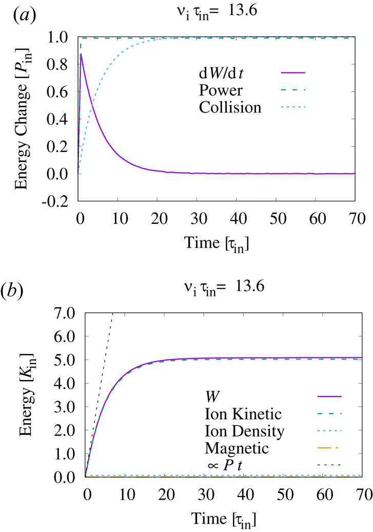
Figure 1 shows the power balance (top) and total energy evolution (bottom). The injected power  $\bar {P}$ measured by the formula (2.24) stays at the given constant value
 $\bar {P}_{\mathrm {in}}$ throughout the run, which confirms the method described in § 2 is correctly implemented and works as desired. Owing to the finite collisionality, the collisional energy dissipation initially increases and reaches the same level as the input, where a statistically steady state is achieved. The energy is mostly dominated by the ion kinetic energy,
 $\sum _{\boldsymbol {k}} m_{{i}} n_{0{i}} |\boldsymbol {u}_{\perp ,{i},\boldsymbol {k}}|^{2}/2$, whereas the density variance of ions,
 $\sum _{\boldsymbol {k}} n_{0{i}}T_{0{i}} |n_{{i},\boldsymbol {k}}/n_{0{i}}|^2/2$ (where
 $n_{{i},\boldsymbol {k}}/n_{0{i}}=\delta n_{{i},\boldsymbol {k}}/n_{0{i}}-q_{{i}} \phi _{\boldsymbol {k}}/T_{0{i}}$), and the magnetic energy,
 $\sum _{\boldsymbol {k}}|\delta B_{\parallel ,\boldsymbol {k}}^2/(2\mu _{0})|$, are small. The total energy initially increases with the energy input rate
 $\bar {P}_{\mathrm {in}}$, and saturates at around 20 eddy times. Note that we set the collision frequency
 $\nu _{\mathrm {ii},\mathrm {ee}}\tau _{\mathrm {in}}\approx 13.6$, therefore particles have experienced sufficient collisions before reaching the steady state. The time to reach the steady state and the saturated energy level depend on how the turbulent spectrum develops, thus are not known a priori. In the current setup, the collisional dissipation is mostly provided by electrons. Thus, if electrons are not kinetic, dissipation does not develop: the total energy of the system unlimitedly increases and a steady state is not achieved. The behaviour of turbulent spectra and how dissipation develops are of central importance to the turbulence study, which we discuss in the next section.
Power balance and energy evolution. The system reaches a statistically steady state where the energy input and collisional dissipation are balanced.

3. Scaling laws of driven gyrokinetic turbulence: from fluid to kinetic regimes
In this section, we demonstrate scaling laws of turbulent fluctuations in both fluid ( $k\rho _{{i}}\ll 1$) and kinetic (
 $k\rho _{{i}}\sim 1$) regimes. The theory of gyrokinetic turbulent cascade was described comprehensively in Schekochihin et al. (Reference Schekochihin, Cowley, Dorland, Hammett, Howes, Quataert and Tatsuno2009). We only consider the case without (kinetic) Alfvén waves and in two dimensions. Plunk et al. (Reference Plunk, Cowley, Schekochihin and Tatsuno2010) specifically focused on gyrokinetic turbulence in two dimensions, and discussed the relation with the Charney–Hasegawa–Mima (CHM) model in the long-wavelength fluid regime. After briefly reviewing the scaling laws derived in those works, we show numerical simulations of driven gyrokinetic turbulence and test if those scalings are established in statistically steady states. We note some essential aspects of the electrostatic gyrokinetic turbulence were already shown in decaying turbulence simulations (Tatsuno et al. Reference Tatsuno, Dorland, Schekochihin, Plunk, Barnes, Cowley and Howes2009, Reference Tatsuno, Barnes, Cowley, Dorland, Howes, Numata, Plunk and Schekochihin2010, Reference Tatsuno, Plunk, Barnes, Dorland, Howes and Numata2012).
In the system considered in this paper, we ignore magnetic perturbation perpendicular to the mean field (no kinetic Alfvén waves). Therefore, the macroscopic system is described by the CHM equation (or Navier–Stokes equation in some limit). In two-dimensional turbulence, a dual cascade of the energy and enstrophy leads to the energy spectrum of  $k^{-3}$ in the inertial range. For a high-
 $\beta$ case, also compressive fluctuations exist which are passively advected by the flow. A transition occurs at the ion kinetic scale. In the kinetic regime, the so-called nonlinear phase mixing starts to play a role, and the behaviour of turbulence changes where turbulent cascades also occur in velocity space. The energy further cascades down to even smaller scales where collisions eventually take out the energy from the system. How the energy is dissipated depends on the particular models of electrons.
3.1. Inertial range
In the long-wavelength limit  $k\rho _{{i}}\ll 1$, the gyro-average acts as unity and
 $\varGamma _{0}(k^{2}\rho _{{i}}^{2}/2)\approx 1-k^{2}\rho _{{i}}^{2}/2$. If we further assume that
 $\beta$ is low (the electrostatic limit) and ions are cold, we reach the well-known CHM equation (Charney Reference Charney1971; Hasegawa & Mima Reference Hasegawa and Mima1977),
 \begin{equation} \frac{\partial }{\partial t} \left(2Q+k^{2}\rho_{{i}}^{2} \right) \phi_{\boldsymbol{k}} - \frac{1}{B_{0}} {\mathcal{F}} \left(\left\{\phi,\rho_{{i}}^{2}\nabla^{2}\phi\right\}\right) = {\mathcal{C}}_{\boldsymbol{k}} + {\mathcal{A}}_{\boldsymbol{k}}, \end{equation}
where  ${\mathcal {C}}_{\boldsymbol {k}} = 2T_{0{i}}/(q_{{i}}n_{0{i}}) \int C_{\boldsymbol {k}} \,\mathrm {d} \boldsymbol {v}$,
 ${\mathcal {A}}_{\boldsymbol {k}} = 2T_{0_{{i}}}/(q_{{i}}n_{0{i}}) \int A_{\boldsymbol {k}}\, \mathrm {d}\boldsymbol {v}$. The parameter
 $Q=Q_{{e}}/Q_{{i}}$ (
 $Q_{s}=q_{s}^{2}n_{0{s}}/T_{0s}$) determines the electron response. The cold ion assumption demands
 $Q \sim k^{2} \rho _{{i}}^{2}$. We immediately find that there are two invariants, the energy and enstrophy, by multiplying (3.1) by
 $\phi _{\boldsymbol {k}}^{\ast }/\rho _{{i}}^{2}$ and
 $k^{2}\phi _{\boldsymbol {k}}^{\ast }/\rho _{{i}}^{2}$,
 \begin{gather} \bar{E}_{\mathrm{CHM}} = \frac{n_{0{i}}m_{{i}}}{2B_{0}^{2}} \sum_{\boldsymbol{k}} \left(\frac{2Q}{\rho_{{i}}^{2}}\left|\phi_{\boldsymbol{k}}\right|^{2} + k^{2}\left|\phi_{\boldsymbol{k}}\right|^{2}\right), \end{gather}
 \begin{gather}\bar{Z}_{\mathrm{CHM}} = \frac{n_{0{i}}m_{{i}}}{2B_{0}^{2}} \sum_{\boldsymbol{k}} \left( \frac{2Q}{\rho_{{i}}^{2}} k^{2} \left|\phi_{\boldsymbol{k}}\right|^{2} + k^{4} \left|\phi_{\boldsymbol{k}}\right|^{2}\right). \end{gather}
Owing to the conservation of energy and enstrophy, a dual cascade will occur in two dimensions: the energy inversely cascades to a larger scale  $k < k_{\mathrm {in}}$, whereas the enstrophy cascades to a smaller scale
 $k>k_{\mathrm {in}}$.
By assuming isotropy and locality of nonlinear interactions, the CHM equation leads to the following relation at each scale  $\ell$,
 \begin{equation} \frac{1}{\tau_{\ell}} \left( 2Q + \frac{\rho_{{i}}^{2}}{\ell^{2}} \right) \sim \frac{1}{B_{0}} \frac{\rho_{{i}}^{2} \phi_{\ell}}{\ell^{4}}, \end{equation}
where  $\tau _\ell$ is the nonlinear decorrelation time. We demand the constancy of the enstrophy flux for the forward cascade:
 \begin{equation} \frac{1}{\tau_{\ell}} \frac{1}{2B_{0}^{2}} \left( \frac{2Q}{\rho_{{i}}^{2}} \frac{\phi_{\ell}^{2}}{\ell^{2}} + \frac{\phi_{\ell}^{2}}{\ell^{4}}\right) \sim \frac{\varepsilon_{Z}}{n_{0{i}}m_{{i}}} = \textrm{const}. \end{equation}
Combining the two relations yields the scaling for  $\phi _{\ell }$
 \begin{equation} \frac{\phi_{\ell}}{B_{0}} \sim \left(\frac{\varepsilon_{Z}}{n_{0{i}}m_{{i}}}\right)^{1/3} \ell^{2}, \end{equation}
which corresponds to the scaling for the energy and enstrophy
 \begin{gather} \frac{\bar{E}_{\mathrm{CHM},k}}{n_{0{i}}m_{{i}}} \sim \left(\frac{\varepsilon_{Z}}{n_{0{i}}m_{{i}}}\right)^{2/3} \left(\frac{2Q}{\rho_{{i}}^{2}} + k^{2} \right) k^{{-}5}, \end{gather}
 \begin{gather}\frac{\bar{Z}_{\mathrm{CHM},k}}{n_{0{i}}m_{{i}}} \sim\left(\frac{\varepsilon_{Z}}{n_{0{i}}m_{{i}}}\right)^{2/3} \left(\frac{2Q}{\rho_{{i}}^{2}} + k^{2} \right)k^{{-}3}. \end{gather}
These scalings indicate that the energy and enstrophy scalings break around  $k\rho _{{i}}\sim \sqrt {2Q}$, where the ion polarisation effect sets in.
In the inverse cascade  $k < k_{\mathrm {in}}$, we demand the constancy of the energy flux,
 $\varepsilon _{E}$,
 \begin{equation} \frac{1}{\tau_{\ell}} \frac{1}{2B_{0}^{2}} \left( \frac{2Q}{\rho_{{i}}^{2}} \phi_{\ell}^{2} + \frac{\phi_{\ell}^{2}}{\ell^{2}} \right) \sim \frac{\varepsilon_{E}}{n_{0{i}}m_{{i}}} = \textrm{const}., \end{equation}
leading to the scaling
 \begin{equation} \frac{\phi_{\ell}}{B_{0}} \sim \left( \frac{\varepsilon_{E}}{n_{0{i}}m_{{i}}}\right)^{1/3} \ell^{4/3}. \end{equation}
We perform gyrokinetic simulations at  $k\rho _{{i}}\ll 1$ with the parameters the same as in § 2.3 except that here
 $\beta _{{i}}=0$. Three types of electron response are examined, namely kinetic, adiabatic (
 $Q=10^{-2}, 10^{-3}$) and zero response (
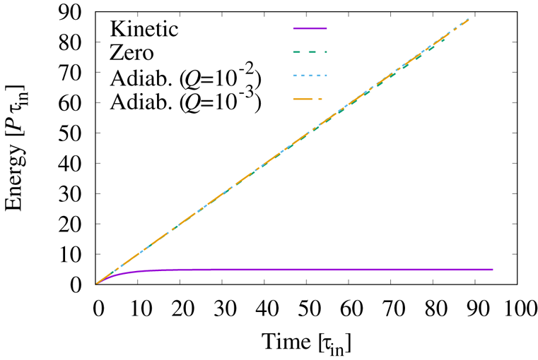
 $Q=0$). Figure 2 shows the time evolution of the generalized energy
 $\bar {W}$. The energy saturates only for the gyrokinetic electron case, whereas it continuously increases during the simulations for other cases.
Time evolution of the energy for the  $k_{\mathrm {in}}\rho _{{i}}=0.02\ll 1$ case. The electron models are gyrokinetic, zero response (
 $Q=0$) and adiabatic response with
 $Q=10^{-2},10^{-3}$. The total energy saturates only for the gyrokinetic electron case.

We then examine the wavenumber spectra after turbulence is fully developed. It is convenient to define the spectrum of  $\bar {W}_{\phi ,k}$
 \begin{equation} \bar{W}_{\phi,k} \,\mathrm{d} k = \frac{q_{{i}}^{2} n_{0{i}}}{2T_{0{i}}} \left|\phi_{\boldsymbol{k}}\right|^{2} \end{equation}
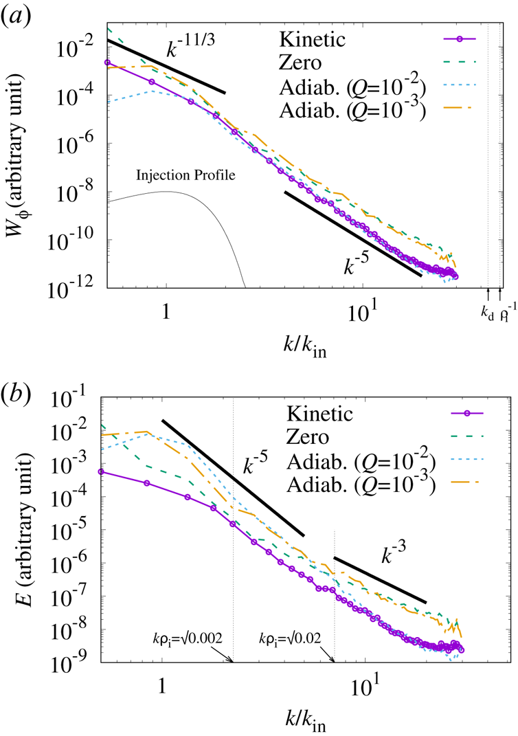
to compare the simulations with the theoretical predictions in this regime as it is irrespective of the electron response. In figure 3, the wavenumber spectra of  $\bar {W}_{\phi ,k}$ and
 $\bar {E}_{\mathrm {CHM},k}$ are shown. The spectra are averages of 100 time snapshots to smooth out temporal variations. The wavenumber is normalized by the injection scale
 $k_{\mathrm {in}}$. From the results of
 $\bar {W}_{\phi ,k}$, we confirm that the theoretical scalings of both the forward (
 $k/k_{\mathrm {in}}>1$) and inverse (
 $k/k_{\mathrm {in}}<1$) cascades are successfully reproduced.Footnote 2 In the figure showing
 $\bar {E}_{\mathrm {CHM},k}$, we depict the transition point
 $k\rho _{{i}}=\sqrt {2Q}$ and the predicted slopes for
 $k\rho _{{i}}\gtrless \sqrt {2Q}$ for reference. Although the transition is not sharp, we observe the slopes at higher and lower wavenumber ranges are different and follow the predictions.
Spectra of  $\bar {W}_{\phi }$ and
 $\bar {E}_{\mathrm {CHM}}$ for the
 $k_{\mathrm {in}}\rho _{{i}}=0.02\ll 1$ case. The gyrokinetic simulation successfully reproduces the scaling laws in the fluid regime.

In the non-gyrokinetic electron cases, the energy inversely cascades to accumulate at a low- $k$ regime. Therefore, there exists no saturation mechanism. However, the accumulated energy is somehow extracted from the system if electrons are gyrokinetic. In fact, the main component of dissipation which balances with the injection is that of electrons. Because the kinetic effect is weak in this small-
 $k$ regime, the electron distribution function is almost Maxwellian, and the collision operator employed in AstroGK (Abel et al. Reference Abel, Barnes, Cowley, Dorland and Schekochihin2008; Barnes et al. Reference Barnes, Abel, Dorland, Ernst, Hammett, Ricci, Rogers, Schekochihin and Tatsuno2009) is dominated by the gyro-diffusion term,
 \begin{equation} C(h_{s}) ={-} \frac{k^{2} \rho_{s}^{2}}{4} ( \nu_{{D}}(1+\xi^{2}) + \nu_{{\parallel}} (1-\xi^{2})) \frac{v^{2}}{v_{\mathrm{th},s}^{2}} h_s, \end{equation}
which acts like friction. Suppose  $h_{s}$ is a Maxwellian,
 \begin{equation} h_{s} = \frac{\delta n_{s}}{n_{0s}} f_{0s}, \end{equation}
the collision term yields
 \begin{equation} \int C(h_{s}) \,\mathrm{d} \boldsymbol{v} ={-} \frac{\sqrt{2}}{3\sqrt{\rm \pi}} \nu_{s} k^{2} \rho_{s}^{2} \delta n_{s}, \end{equation}
which corresponds to a friction force in the vorticity equation. Therefore, the large scale flow can be decelerated to reach the steady state if the electron collision is incorporated.
3.2. Ion entropy cascade
On a smaller scale, ions follow the gyrokinetic equation where the nonlinear phase mixing leads to the cascade of entropy. We consider a scale  $\rho _{{e}}\ll \ell \ll \rho _{{i}}$. The energy flux at
 $\ell$ is given by
 \begin{equation} \varepsilon \sim \frac{n_{0{i}}m_{{i}}v_{\mathrm{th},{i}}^{2}}{4\tau_{\ell}} \left(\frac{h_{{i},\ell}v_{\mathrm{th},{i}}^{3}}{n_{0{i}}}\right)^{2}= \textrm{const}. \end{equation}
From the gyrokinetic equation, the nonlinear decorrelation time is estimated as
 \begin{equation} \frac{1}{\tau_{\ell}} \sim \frac{1}{B_{0}} \frac{1}{\ell^{2}} \left\langle \phi \right\rangle_{\boldsymbol{R}} \sim \frac{1}{B_{0}} \frac{\phi_{\ell}}{\ell^{2}} \left(\frac{\rho_{{i}}}{\ell}\right)^{{-}1/2}. \end{equation}
The gyro-averaging operation introduces a reduction factor  $(\rho _{{i}}/\ell )^{-1/2}$. Note that
 $A_{\parallel }\approx 0$. From the quasi-neutrality for the Boltzmann response electron,
 \begin{equation} \frac{q_{{i}}\phi_{\ell}}{T_{0{i}}} \left(1+Q\right) \sim \frac{v_{\mathrm{th},{i}}^{3}}{n_{0{i}}} h_{{i},\ell} \left( \frac{\rho_{{i}}}{\ell} \right)^{{-}1/2} \left( \frac{\delta v}{v_{\mathrm{th},{i}}}\right)^{1/2}. \end{equation}
The nonlinear phase mixing produces structures in velocity space correlated with the spatial scale,
 \begin{equation} \frac{\delta v}{v_{\mathrm{th},{i}}} \sim \frac{\ell}{\rho_{{i}}}. \end{equation}
Combining all the relations, we obtain
 \begin{equation} \frac{\varepsilon}{n_{0{i}}m_{{i}}} \sim \frac{v_{\mathrm{th},{i}}^{12}}{8n_{0{i}}^{3}} \left(1+Q\right)^{{-}1} \ell^{{-}1/2}\rho_{{i}}^{{-}1/2} h_{{i},\ell}^{3}. \end{equation}
This gives a scaling for  $h_{{i},\ell }$ as
 \begin{equation} h_{{i},\ell} \sim \frac{n_{0{i}}}{v_{\mathrm{th},{i}}^{4}} \left(1+Q\right)^{1/3} \left(\frac{\varepsilon}{n_{0{i}}m_{{i}}}\right)^{1/3} \ell^{1/6}\rho_{{i}}^{1/6}. \end{equation}
Scalings for  $\phi _{\ell }$ and
 $\tau _{\ell }$ are similarly given by
 \begin{gather} \phi_{\ell}/B_0 \sim \left(1+Q\right)^{{-}2/3} \left(\frac{\varepsilon}{n_{0{i}}m_{{i}}}\right)^{1/3} \ell^{7/6} \rho_{{i}}^{1/6}, \end{gather}
 \begin{gather}\tau_{\ell} \sim \left(1+Q\right)^{2/3} \left(\frac{\varepsilon}{n_{0{i}}m_{{i}}}\right)^{{-}1/3} \ell^{1/3} \rho_{{i}}^{1/3}. \end{gather}
The energy scalings follow from these as
 \begin{gather} W_{h,k} \,\mathrm{d} k = \int \frac{T_{0{i}}\left|h_{{i},k}\right|^{2}}{2f_{0{i}}} \,\mathrm{d} \boldsymbol{v} \sim n_{0{i}} m_{{i}} \left(1+Q\right)^{2/3} \left(\frac{\varepsilon}{n_{0{i}}m_{{i}}}\right)^{2/3} k^{{-}1/3} \rho_{{i}}^{1/3}, \end{gather}
 \begin{gather}W_{\phi,k} \,\mathrm{d} k = \frac{q_{{i}}^{2} n_{0{i}}}{2T_{0{i}}} \left|\phi_{k}\right|^{2} \sim n_{0{i}} m_{{i}} \left(1+Q\right)^{{-}4/3} \left(\frac{\varepsilon}{n_{0{i}}m_{{i}}}\right)^{2/3} k^{{-}7/3} \rho_{{i}}^{{-}5/3}. \end{gather}
The collisional cutoff scale in Fourier space  $k_{{d}}$ and in velocity space
 $\delta v_{{d}}$ is estimated by balancing the cascade time and collisional time scale,
 \begin{equation} \nu_{\mathrm{ii}} v_{\mathrm{th},{i}}^{2} \left(\frac{\partial }{\partial v}\right)^{2} \sim \tau_{\ell}^{{-}1}. \end{equation}
Substituting the relations (3.18) and (3.22) at  $\ell ^{-1}=k_{{d}}$, we obtain
 \begin{equation} k_{{d}}\rho_{{i}} \sim (\nu_{\mathrm{ii}}\tau_{\rho_{{i}}})^{{-}3/5} \sim D^{3/5}, \end{equation}
where the dimensionless number defined by
 \begin{equation} D=(\nu_{\mathrm{ii}}\tau_{\rho_{{i}}})^{{-}1}, \end{equation}
is called the Dorland number characterizing the range of ion kinetic scale in velocity space as well as in Fourier space. Setting  $\ell =\rho _{{i}}$ in (3.22), we obtain
 \begin{equation} D \sim \nu_{\mathrm{ii}}^{{-}1} (1+Q)^{{-}2/3} \left( \frac{\varepsilon}{n_{0{i}}m_{{i}}}\right)^{1/3} \rho_{{i}}^{{-}2/3}. \end{equation}
To study turbulence in the ion kinetic regime, we take the injection scale at the ion Larmor radius  $k_{\mathrm {in}}\rho _{{i}}=2$. To reduce the effect of the inverse cascade, we set the box size as
 $k_{\mathrm {in}}L=1$. Other parameters are the same as those in the previous section. We perform simulations for three values of
 $\nu _{\mathrm {ii}}$ corresponding to (i)
 $D=79.4$, (ii)
 $D=159$ and (iii)
 $D=397$ to vary
 $k_{{d}}\rho _{{i}}$. In the estimation of
 $D$, we set
 $Q=0$ and
 $\varepsilon =\bar {P}_{\mathrm {in}}$ for simplicity. The gyrokinetic and zero response electron models are used. For all cases, the resolution in the
 $x$–
 $y$ plane is
 $128^{2}$ and that in velocity space is
 $64^{2}$ for cases (i) and (ii) and
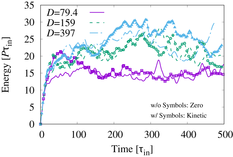
 $128^{2}$ for case (iii). The time evolution of the generalized energy in figure 4 confirms that the system reaches steady states for all cases. In this ion kinetic scale, the ion entropy cascade occurs in velocity space until
 $\delta v$ extends to the scale where the collisional dissipation of ions (proportional to
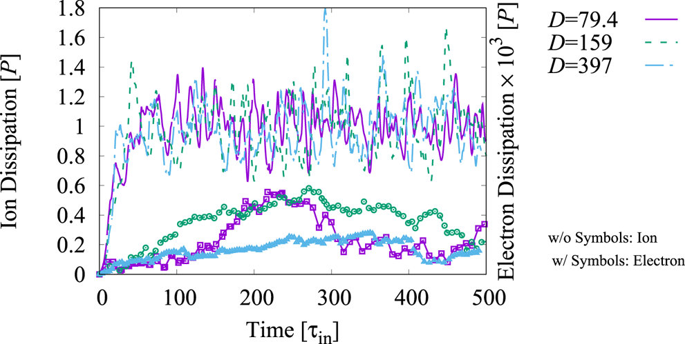
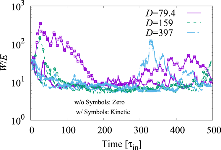
 $\nu _{\mathrm {ii}} \delta v^{2}$) balances with the input, namely the injected energy is completely taken out from the system at the ion scale. As long as the sufficiently large resolution is taken in both real and velocity spaces, the steady state is achieved. We see that there is not much difference between the zero response and gyrokinetic electron cases. For the gyrokinetic case, the electron dissipation is much smaller than that of ions (figure 5). In figure 6, we plot the ratio of the generalized energy to the electrostatic invariant,
 $W/E$. The ratio seems approaching to some constant value (
 ${\sim }10$) regardless of the parameters. This fact may have some implications to the nature of inverse cascades, which will be studied elsewhere.
Time evolution of the energy for the  $k_{\mathrm {in}}\rho _{{i}}=2=O(1)$ case. Three cases of
 $D$ values with two electron models are simulated. There is not much difference between zero response and gyrokinetic electrons.

Time evolution of the dissipation for the  $k_{\mathrm {in}}\rho _{{i}}=2=O(1)$ case. The ion dissipation behaves similarly for both electron response cases, so only the gyrokinetic electron case is shown. The electron dissipation, which exists only in the gyrokinetic case, is much smaller than that of ions. Note that the electron dissipation is magnified by a factor of
 $10^{3}$.

The ratio of the generalized energy to the electrostatic invariant  $W/E$.

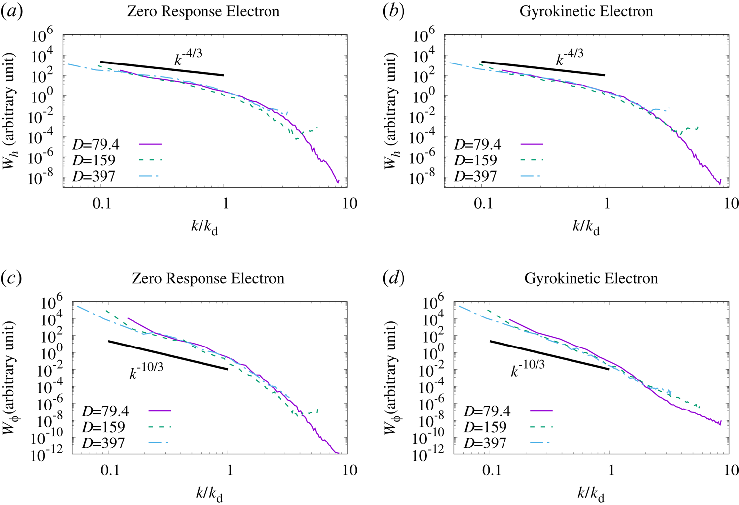
Figure 7 shows the wavenumber spectra of  $\bar {W}_{h}$ and
 $\bar {W}_{\phi }$. Although both electron response cases are shown in separate plots, we again note that the spectra of the ion entropy cascade (as well as the temporal evolution of the energy) are indifferent to the electron response. The wavenumber is normalized by the dissipation cutoff scale
 $k_{{d}}$. For all cases, the spectra start to fall off around
 $k\sim k_{{d}}$. Here
 $k_{{d}}$ gives a good measure of the dissipation scale. For the largest
 $D$,
 $k_{{d}}\rho _{{i}}\sim 36.2$ and the range of injection and dissipation are separated. We see spectra roughly consistent with the theory in the range
 $k/k_{{d}}<0.5$ although the dynamic range is quite narrow.
Wavenumber spectra of  $\bar {W}_{h}$ and
 $\bar {W}_{\phi }$. The zero response and gyrokinetic electron models are shown.

We do not reproduce all the detail of the entropy cascade dynamics, such as velocity space spectra, entropy transfer and just remark that they are almost the same as those for the well-established decaying turbulence case. Interested readers are referred to the work by Tatsuno et al. (Reference Tatsuno, Dorland, Schekochihin, Plunk, Barnes, Cowley and Howes2009, Reference Tatsuno, Barnes, Cowley, Dorland, Howes, Numata, Plunk and Schekochihin2010, Reference Tatsuno, Plunk, Barnes, Dorland, Howes and Numata2012). The virtue of the driven case developed here is that simulations are set up in a controlled manner where the injection and dissipation scales are fixed, and long-time statistics can be discussed in a steady state if necessary.
3.3. Compressive fluctuations in high- $\beta$ plasmas

In high- $\beta$ cases, compressive fluctuations involving
 $\delta B_{\parallel }$ are also induced. The parallel magnetic fluctuation is given by
 \begin{equation} \frac{\delta B_{{\parallel},\boldsymbol{k}}}{B_{0}} ={-} \frac{\beta_{{i}}}{2} \frac{1}{n_{0{i}}}\int \frac{2v_{{\perp}}^{2}}{v_{\mathrm{th},{i}}^{2}} \frac{\textrm{J}_{1}{i}}{\alpha_{{i}}} h_{{i},\boldsymbol{k}}\,\mathrm{d} \boldsymbol{v}, \end{equation}
if electrons follow the Boltzmann relation ( $h_{{e}}=0$). The magnetic fluctuations are small compared with
 $q_{{i}} \phi /T_{0{i}}$ by a factor of
 $\beta _{{i}}/(k\rho _{{i}})$. By employing a similar argument, we obtain a scaling law for the magnetic fluctuation,
 \begin{gather} \frac{\delta B_{{\parallel},\ell}}{B_{0}} \sim \beta_{{i}} \frac{1}{v_{\mathrm{th},{i}}} \left(1+Q\right)^{1/3} \left( \frac{\varepsilon}{n_{0{i}}m_{{i}}} \right)^{1/3} \ell^{13/6} \rho_{{i}}^{{-}11/6}, \end{gather}
 \begin{gather}\bar{M}_{{\parallel},k} \,\mathrm{d} k = \frac{\left|\delta B_{{\parallel},k}\right|^{2}}{2\mu_{0}} \sim n_{0{i}} m_{{i}} \beta_{{i}} \left( 1 + Q \right)^{2/3} \left( \frac{\varepsilon}{n_{0{i}}m_{{i}}}\right)^{2/3} k^{{-}13/3} \rho_{{i}}^{{-}11/3}. \end{gather}
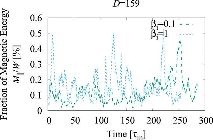
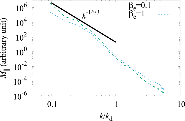
We include finite  $\beta _{{i}}=0.1, 1$ for the
 $D=159$ case, and observe the spectrum of
 $\bar {M}_{\parallel }$. Figure 8 shows the fraction of parallel magnetic energy to the total energy. The magnetic energy stays at a negligible level throughout the simulation. The magnetic energy spectrum shown in figure 9 agrees well with the theoretical predicted scaling
 $k^{-16/3}$ for any values of
 $\beta _{{i}}$.
Time evolution of the fraction of magnetic energy to total energy  $M_{\parallel }/W$.

Wavenumber spectra of  $M_{\parallel }$.

As the compressive fluctuations are small, they do not affect the flow dynamics, and behave as a passive scalar even though they are essentially coupled with the flows in this kinetic regime. When  $\beta$ gets even higher, the magnetic fluctuations may become comparable to other components and start to affect the flows. This result may be compared with the compressive fluctuations in Alfvénic turbulence observed in solar winds and simulations of the electromagnetic plasma turbulence. The long-standing puzzle of the magnetic fluctuations in solar winds (Marsch & Tu Reference Marsch and Tu1990; Chen Reference Chen2016) is that they do not damp and have the scaling similar to the fluid. It is argued that the stochastic plasma echo inhibits phase mixing so that plasmas behave more fluid-like (fluidisation) (Schekochihin et al. Reference Schekochihin, Parker, Highcock, Dellar, Dorland and Hammett2016; Meyrand et al. Reference Meyrand, Kanekar, Dorland and Schekochihin2019), thus follow shallower spectra than the kinetic one (3.31). The present result showing the kinetic nature of turbulence shows a marked difference with the Alfvénic case. We remark that here the Landau damping mechanism of compressive fluctuations along the mean magnetic field is absent.
4. Summary
We have constructed an external forcing term to drive turbulence in two-dimensional electromagnetic gyrokinetics and have implemented it in AstroGK code. The additional term in the gyrokinetic equation describing the temporal evolution of distribution functions induces density and temperature fluctuations of plasmas, and thus disturbs the electrostatic potential and magnetic field parallel to the mean magnetic field through the quasi-neutrality and pressure balance equations. The induced electrostatic potential corresponds to the  $\boldsymbol {E} \times \boldsymbol {B}$ velocity, therefore the term is equivalent to the ‘forcing’ (drives flows) in the reduced MHD equations. By construction, the newly introduced term does not excite the magnetic field perpendicular to the mean magnetic field. The Alfvén wave is completely absent in the present work.
By the external drive, stationary turbulence is numerically generated in a controlled manner to study the statistical properties of fluctuations. The two essential properties of the forcing are locality in the wavenumber space and a pre-determined energy injection rate. To fix an energy injection rate, the force is chosen to make the force–velocity correlation vanish. These properties enable turbulence to be set up in any dynamical scales ranging from the injection scale  $k_{\mathrm {in}}$ set by the forcing term to the dissipation scale
 $k_{{d}}$ determined by the injected power and dissipation parameter (collisionality). We have performed two simulations, namely in the large-scale fluid regime and small-scale ion kinetic regime.
In the fluid regime ( $k_{\mathrm {in}} \rho _{{i}}\ll 1$), we have shown the forward enstrophy and inverse energy cascade by gyrokinetic simulations, and have successfully produced the theoretical scalings of the wavenumber spectra. We have also demonstrated the breaking of the wavenumber spectra due to the ion polarisation effect, corresponding to the CHM turbulence. These results are all well studied using fluid models, and there is no reason to employ computationally demanding kinetic description. However, we emphasize that the ability to correctly capture large-scale behaviour using the kinetic model is still useful for studying the connection of fluid models and kinetic models, and also for performing holistic simulations including all microphysics to macro-scale dynamics. We note that in the fluid regime, it is a subtle issue to achieve a stationary state because ignoring small scales prevents collisional dissipation from developing to balance the injection.
In the kinetic regime ( $k_{\mathrm {in}} \rho _{{i}} \sim 1$), we have studied the ion entropy cascade turbulence. In this regime, the nonlinear phase mixing due to the finite Larmor radius effect creates structures in velocity space. The ion entropy cascade carries the injected energy to small scales in both real and velocity spaces, and eventually ceases at the dissipation cutoff scale due to collisions. It is found that the ion collisional dissipation balances with the injected energy in this regime. The obtained scalings agree well with the theoretical prediction and with decaying turbulence simulations which were previously done. In addition to the electrostatic case, we have also performed simulations of high-
 $\beta$ plasmas where compressive fluctuations involving magnetic fields parallel to the mean field are also excited. It is confirmed that the compressive fluctuations are just passively advected by the flow, and do not affect the scaling laws of turbulence as long as
 $\beta$ is not too high.
The simulations performed in this work are in four-dimensional phase space (two each in real and velocity spaces), and the resolution is up to  $O(10^2)$ in each direction, which is relatively low compared with the cutting edge numerical simulations. We admit the dynamic range is not sufficiently wide to observe clear spectra because of the restriction of numerical resources, although we do capture the essential features of generated turbulence. It is acceptable for the testing purpose of the development of the forcing method.
The turbulence generated by the forcing method presented here is restricted to two dimensions and the case without Alfvén waves on purpose. Such a situation may occur in realistic plasmas because there are several energy cascade channels from the macroscopic to kinetic scales, and it is not known on which paths the cascades take place depending on situations. The current study focusing on a specific situation still contributes to the comprehensive understanding of kinetic plasma turbulence. In the future, we apply this work for the situation in the presence of an initial magnetic field and magnetic reconnection, which provides another energy dissipation mechanism. As the relative strength of turbulence compared with magnetic reconnection is measurable, the developed method enables quantitative analyses of energy dissipation in the co-existing system of turbulence and magnetic reconnection.
Acknowledgements
The author would like to thank W. Dorland, Y. Kawazura, N. F. Loureiro, G. Plunk and T. Tatsuno for their fruitful comments. The computation of this work is performed on the facilities of the Center for Cooperative Work on Computational Science, University of Hyogo, the JFRS-1 supercomputer system at the Computational Simulation Centre of the International Fusion Energy Research Centre (IFERC-CSC) in Rokkasho Fusion Institute of QST (Aomori, Japan) and on the ‘Plasma Simulator’ of NIFS with the support and under the auspices of the NIFS Collaboration Research program (NIFS18KNSS112).
Editor William Dorland thanks the referees for their advice in evaluating this article.
Declaration of interests
The author reports no conflict of interests.
Appendix A. Gyrokinetic–Maxwell equations
In this paper, we implement an additional forcing term in AstroGK. We briefly describe the gyrokinetic-Maxwell equations used in the code. (See Numata et al. (Reference Numata, Howes, Tatsuno, Barnes and Dorland2010) for the complete description of the model.) AstroGK solves the nonlinear, local flux tube,  $\delta f$, electromagnetic gyrokinetic equation. It determines fluctuating fields of the species
 $s$ around a Maxwellian background in the mean magnetic field
 $\boldsymbol {B}_{0}=B_{0}\boldsymbol {z}$ defined by
 $n_{0s}$ and
 $T_{0s}$:
 $f_{0s}=n_{0s}/(\sqrt {{\rm \pi} }v_{\mathrm {th},s})^{3} \exp (-v^2/v_{\mathrm {th},s}^{2})$ with
 $v_{\mathrm {th},s}=\sqrt {2T_{0s}/m_{s}}$ being the thermal velocity. For the sake of simplicity, we only consider two-dimensional (
 $\partial /\partial _{z}=0$) and uniform plasmas.
The gyrokinetic equation determines the evolution of  $g_{s}$ in Fourier space
 \begin{equation} \frac{\partial g_{\boldsymbol{k},s}}{\partial t} + \frac{1}{B_{0}} {\mathcal{F}}\left( \left\{ \langle \chi \rangle_{\boldsymbol{R}_{s}}, h_{s} \right\}\right) = \frac{q_{s} f_{0s}}{T_{0s}} v_{{\parallel}} \textrm{J}_{0s} \frac{\partial A_{{\parallel},\boldsymbol{k}}}{\partial t} + C_{\boldsymbol{k}} (h_{\boldsymbol{k},s}), \end{equation}
where  $g_{s}$ is defined using the non-Boltzmann part of the perturbed distribution function
 $h_{s} = \delta f_{s} + (q_{s} \phi /T_{0s}) f_{0s}$ as
 \begin{equation} g_{\boldsymbol{k},s} = h_{\boldsymbol{k},s} - \frac{q_{s} \phi_{\boldsymbol{k}}}{T_{0s}} \textrm{J}_{0s} f_{0s} - \frac{2v_{{\perp}}^{2}}{v_{\mathrm{th},s}^{2}} \frac{\textrm{J}_{1s}}{\alpha_{s}} f_{0s} \frac{\delta B_{{\parallel},\boldsymbol{k}}}{B_{0}}. \end{equation}
Note that  $\boldsymbol {k}=(k_{x},k_{y})$ is the wavenumber in the plane perpendicular to
 $\boldsymbol {B}_{0}$. The distribution function
 $g_{s}$ and field variables (e.g.
 $\phi$) are decomposed, respectively, in the gyro-centre coordinate
 $\boldsymbol {R}_{s}$ and particle coordinate
 $\boldsymbol {r}$ as
 \begin{gather} g_{s} = \sum_{\boldsymbol{k}} g_{\boldsymbol{k},s} \,\textrm{e}^{\mathrm{i} \boldsymbol{k}\boldsymbol{\cdot}\boldsymbol{R}_{s}}, \end{gather}
 \begin{gather}\phi = \sum_{\boldsymbol{k}} \phi_{\boldsymbol{k}} \,\textrm{e}^{\mathrm{i} \boldsymbol{k}\boldsymbol{\cdot}\boldsymbol{r}}. \end{gather}
The coordinate transform is given by
 \begin{equation} \boldsymbol{R}_{s} = \boldsymbol{r} - \frac{\boldsymbol{v}\times\boldsymbol{B}_{0}}{\varOmega_{s}} \quad (\varOmega_{s}\textrm{: cyclotron frequency}). \end{equation}
The Bessel function of the first kind  $\textrm {J}_{ns}=\textrm {J}_{n}(\alpha _s)$ with the argument
 $\alpha _{s}=|\boldsymbol {k}|v_{\perp }/\varOmega _{s}$ arises from the coordinate transformation via the gyro-averaging operation.
Three field variables,  $\phi$,
 $A_{\parallel }$ and
 $\delta B_{\parallel }$, satisfy the Maxwell equations:
 \begin{gather} \left[ \sum_{s} \frac{q_{s}^{2}n_{0s}}{T_{0s}}\left(1-\varGamma_{0s}\right) \right] \phi_{\boldsymbol{k}} - \left[ \sum_{s} q_{s} n_{0s} \varGamma_{1s} \right] \frac{\delta B_{{\parallel},\boldsymbol{k}}}{B_{0}} = \sum_{s} q_{s} \int \textrm{J}_{0}{s} g_{\boldsymbol{k},s} \,\mathrm{d} \boldsymbol{v}, \end{gather}
 \begin{gather}k^{2} A_{{\parallel},\boldsymbol{k}} = \mu_{0} \sum_{s} q_{s} \int v_{{\parallel}} \textrm{J}_{0}{s} g_{\boldsymbol{k},s} \,\mathrm{d} \boldsymbol{v}, \end{gather}
 \begin{gather}\left[ \sum_{s} q_{s}n_{0s} \varGamma_{1s} \right] \phi_{\boldsymbol{k}} + \left[ \frac{B_{0}^{2}}{\mu_{0}} + \sum_{s} n_{0s} T_{0s} \varGamma_{2s} \right] \frac{\delta B_{{\parallel},\boldsymbol{k}}}{B_{0}} ={-} \sum_{s} \int m_{s} v_{{\perp}}^{2} \frac{\textrm{J}_{1}{s}}{\alpha_{s}} g_{\boldsymbol{k},s}\, \mathrm{d} \boldsymbol{v}. \end{gather}
The function  $\varGamma _{ns}=\varGamma _{n}(b_{s})$ is given by
 \begin{gather} \varGamma_{0s} = \textrm{I}_{0}(b_{s})\, \textrm{e}^{{-}b_{s}}, \end{gather}
 \begin{gather}\varGamma_{1s} = \left(\textrm{I}_{0}(b_{s}) - \textrm{I}_{1}(b_{s})\right) \textrm{e}^{{-}b_{s}}, \end{gather}
 \begin{gather}\varGamma_{2s} = 2 \varGamma_{1s}, \end{gather}
where  $\textrm {I}_{n}$ is the modified Bessel function of the first kind, and the argument is
 $b_{s}=(|\boldsymbol {k}|\rho _{s})^{2}/2$ (
 $\rho _s$ is the Larmor radius).
We introduce the following symbols for notational simplicity.
 \begin{equation} \boldsymbol{\mathsf{Y}} = \begin{pmatrix} {{\mathsf{Y}}}_{1} & -{{\mathsf{Y}}}_{3} \\ {{\mathsf{Y}}}_{3} & {{\mathsf{Y}}}_{2} \end{pmatrix} = \begin{pmatrix} \sum\limits_{s} \dfrac{q_{s}^{2}n_{0s}}{T_{0s}} \left(1-\varGamma_{0s}\right) & - \sum\limits_{s} q_{s} n_{0s} \varGamma_{1s} \\ \sum\limits_{s} q_{s} n_{0s} \varGamma_{1s} & \dfrac{B_{0}^{2}}{\mu_{0}} + \sum\limits_{s} n_{0s} T_{0s} \varGamma_{2s} \end{pmatrix}. \end{equation}
Then, the coupled field equations for  $\phi$ and
 $\delta B_{\parallel }$ are given by
 \begin{equation} \begin{pmatrix} {{\mathsf{Y}}}_{1} & - {{\mathsf{Y}}}_{3} \\ {{\mathsf{Y}}}_{3} & {{\mathsf{Y}}}_{2} \end{pmatrix} \begin{pmatrix} \phi_{\boldsymbol{k}} \\ \dfrac{\delta B_{{\parallel},\boldsymbol{k}}}{B_{0}} \end{pmatrix} = \begin{pmatrix} \sum\limits_{s} q_{s} \int \textrm{J}_{0}{s} g_{\boldsymbol{k},s} \,\mathrm{d} \boldsymbol{v} \\ - \sum\limits_{s} q_{s} \int m_{s} v_{{\perp}}^{2} \dfrac{\textrm{J}_{1}{s}}{\alpha_{s}} g_{\boldsymbol{k},s} \,\mathrm{d} \boldsymbol{v} \end{pmatrix}. \end{equation}
In some cases, we do not solve the gyrokinetic equation for electrons and just assume the zero response ( $\delta f_{{s}}=0$ ) or the adiabatic (or Boltzmann) response (
 $h_{{e}}=0$). In either case, the electron response is parameterized by
 $Q_{{e}}$, where
 \begin{equation} \boldsymbol{\mathsf{Y}} = \begin{pmatrix} Q_{{e}} + \dfrac{q_{{i}}^{2} n_{0{i}}}{T_{0{i}}} \left(1-\varGamma_{0{i}}\right) & - q_{{i}} n_{0{i}} \varGamma_{0{i}} \\ q_{{i}} n_{0{i}} \varGamma_{0{i}} & \dfrac{B_{0}^{2}}{\mu_{0}} + n_{0{i}} T_{0{i}} \varGamma_{2{i}} \end{pmatrix}. \end{equation}
For the zero response case,  $Q_{{e}}=0$, whereas for the adiabatic response case,
 $Q_{{e}}=q_{{e}}^{2} n_{0{e}}/T_{0{e}}$. The right-hand side of the field equations should also change accordingly (
 $g_{\boldsymbol {k},{e}}=0$).
Other non-standard symbols that are not explained in the text are summarized in table 1.
Explanation of non-standard symbols.