Introduction
Strong near-surface winds are the most prominent atmospheric features around the coast of Antarctica. Many previous studies have shown that most of these winds are caused by topography associated with strong katabatic winds (Parish Reference Parish1984, Parish & Waight Reference Parish and Waight1987, Parish & Cassano Reference Parish and Cassano2003), synoptic-scale low-pressure systems moving along the Antarctic coastal regions (Simmonds & Keay Reference Simmonds and Keay2000) or a combined effect of these two factors (Parish & Bromwich Reference Parish and Bromwich1998, van den Broeke & van Lipzig Reference Van den Broeke and van Lipzig2003, Turner et al. Reference Turner, Chenoli, Samah, Marshall, Phillips and Orr2009). In addition to these two main causes, strong winds can result from the complex orography that gives rise to barrier winds and mountain waves. Nigro et al. (Reference Nigro, Cassano, Lazzara and Keller2012) investigated a strong wind event observed at the Sabrina Automatic Weather Station (AWS) over the Ross Ice Shelf and revealed that forcing associated with the barrier wind corner jet to the north-west of the Prince Olav Mountains was the major factor in controlling the maximum wind speed. Steinhoff et al. (Reference Steinhoff, Bromwich, Lambertson, Knuth and Lazzara2008) and Chenoli et al. (Reference Chenoli, Turner and Samah2015) showed that downslope windstorms caused by the topography of Mina Buff and Black Island are among the factors contributing to the occurrence of strong winds at McMurdo, West Antarctica. Orr et al. (Reference Orr, Phillips, Webster, Elvidge, Weeks, Hosking and Turner2014) showed that strong wind events at Mawson, East Antarctica, were the result of the barrier jet and downslope windstorm caused by the topography around Mawson, together with a strengthening of the katabatic flow associated with the approach of a deep depression towards the coast. Recently, Kwon et al. (Reference Kwon, Park, Lee, Kim, Choi and Kim2019) investigated the characteristics of a strong wind event at King Sejong Station (KSJ) located on the Antarctic Peninsula (AP) region using numerical model experiments and observational data analysis. They revealed that winds at KSJ were intensified by downslope windstorms at the leeward side of the AP as a deep cyclonic system approached.
As outlined above, several previous studies have stressed the role of topography on strong wind events over Antarctica. However, the effect of topography on the occurrence of strong winds has not yet been quantified. In this study, as an extension of earlier research by Kwon et al. (Reference Kwon, Park, Lee, Kim, Choi and Kim2019), we attempt to quantify the effect of AP topography on a strong wind event at KSJ through numerical experiments applying different terrain heights. The AP is a high and narrow mountain ridge that reaches > 2 km in altitude and runs for ~1500 km in length. It is orientated approximately from north to south and is bounded by the Antarctic continent (Grosvenor et al. Reference Grosvenor, King, Choularton and Lachlan-Cope2014). The shape of this topography probably affects the surrounding environment, including near-surface winds.
The wind at KSJ generally shows a weak seasonal cycle throughout the year due to the year-round frequent passage of low-pressure systems. The climatological value of monthly mean wind speeds for the period from 1989 to 2015 varies from small values during summer (~6.7 m/s) to large values in winter (~9 m/s) (Kwon et al. Reference Kwon, Park, Lee, Kim, Choi and Kim2019). It exhibits small monthly differences of ~2–3 m/s. In addition, the north-westerly winds prevail for this region throughout the year. The strong wind event occurred at KSJ on 7 January 2013 lasted for almost 12 h, from 06h40 to 18h50 UTC, and it was recorded as a blizzard with daily mean wind speeds of ~16 m/s in the weather report. The wind direction varied from ~100° to 150°, showing mainly a south-easterly direction. At KSJ, winds are typically weaker during the summer (January), with the daily climatology of wind speed being ~6.7 m/s during the period from 1994 to 2015 (Kwon et al. Reference Kwon, Park, Lee, Kim, Choi and Kim2019). The daily mean wind speed exceeds 8 m/s from April (mid-autumn) to October (spring). The maximum of daily mean wind speed (~10.6 m/s) is usually recorded in August (winter), when mesoscale cyclone activities around Antarctica are most prominent. During 6–8 January 2013, a peak value of average 10 min wind speed and a maximum instantaneous wind speed were recorded as 21.9 and 41.0 m/s, respectively. Therefore, as an anomaly in summer, the event is obviously extreme and unusual compared to the climatological wind at KSJ. Only two strong wind cases with maximum instantaneous wind speeds > 41.0 m/s have been recorded during the summer since the establishment of KSJ in 1988. Considering the frequency distribution of the daily maximum value of instantaneous 10 m wind speed for 2005–2015, a daily maximum instantaneous wind speed of 41.0 m/s occurs with a chance of < 0.88% (Kwon et al. Reference Kwon, Park, Lee, Kim, Choi and Kim2019). In addition, an important characteristic of this strong wind event is the south-easterly wind direction going over the AP topography. South-easterly winds are very rare at KSJ throughout the year (~4%). Northerly, westerly and north-westerly winds generally prevail for this region during all seasons (~52%). In addition, strong wind events at KSJ do not always occur during south-easterly winds. Kwon et al. (Reference Kwon, Park, Lee, Kim, Choi and Kim2019) examined the characteristics of extreme wind events at KSJ. They analysed the wind direction for 22 extreme strong wind cases of > 41.0 m/s of maximum instantaneous wind speeds and showed that the 22 strong wind cases are divided into two groups of major wind directions: easterly (90–150°; 13 cases) and northerly (326–360°, 0–33°; 9 cases).
The following section describes the data and methodology for the numerical experiments. The results of the numerical experiments with and without AP topography are then discussed. Finally, a summary and conclusions are presented.
Data and methods
Data
The data obtained from the Automatic Meteorological Observation System (AMOS) in operation at KSJ from 1989 to 2015 were used to validate strong wind simulations by comparing model outputs at the nearest model grid to observations. The AMOS consists of a wind vane and an anemometer at a height of 10 m, a thermo-hygrometer at an elevation of ~2 m and a rain gauge and barometer at ~1.5 m above the ground (Park et al. Reference Park, Choi and Kim2013). The data were measured by each sensor at an interval of 1 or 10 s, depending on the parameter of interest, and they are averaged once every 10 min and stored in the data recorder (Kwon et al. Reference Kwon, Park, Lee, Kim, Choi and Kim2019). Hourly mean observation of 10 m wind speeds and directions, sea-level pressures and 2 m air temperature were used to evaluate the model simulation results.
Model configurations
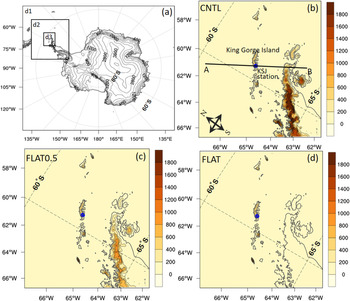
To examine the AP topography effect on the chosen strong wind event, the Polar WRF model version 3.7 (Hines & Bromwich Reference Hines and Bromwich2008) was used. The Polar WRF is an optimized version of the WRF (Powers et al. Reference Powers, Klemp, Skamarock, Davis, Dudhia and Gill2017) specifically for polar regions and better represents key regional physical processes; it includes enhancements of the sea-ice, snowpack and cloud radiative processes over the polar regions (Hines & Bromwich Reference Hines and Bromwich2008). Three model domains with horizontal resolutions of 27 (281 × 242 grid points), 9 (202 × 220 grid points) and 3 km (187 × 205 grid points) were designed in order to examine the sensitivity of wind strength to topography (Fig. 1). The outermost domain with a horizontal resolution of 27 km covers the entire Antarctic continent, while two nested subdomains progressively cover the region of the AP in which KSJ is located. The model includes 61 vertical levels from the surface to 10 hPa. The 6 hourly European Centre for Medium-range Weather Forecasting (ECMWF) Interim reanalysis data with a horizontal resolution of 0.75° latitude and 0.75° longitude were used to provide initial and boundary conditions for numerical simulations. The default United States Geological Survey (USGS) 24 category land use data and global 30'' elevation data were used to provide land type and topography information for model runs.
a. Polar Weather Research and Forecasting domain at horizontal resolutions of 27 (d1), 9 (d2) and 3 km (d3) with topographical elevation contours (400 m intervals). b. Enlarged view of the 3 km domain (d3 for the CNTL experiment) with terrain heights (colour shading, m). The blue circle indicates the location of King Sejong Station. The line from A to B indicates the location of the vertical cross-section of potential temperature and wind speed shown in Fig. 7. c. and d. are the same as b., except for the FLAT0.5 and FLAT experiments, respectively.

The physics schemes used in the present numerical experiments included the WRF Single Moment 5-class (WSM5) microphysics (Hong et al. Reference Hong, Dudhia and Chen2003), the new version of the rapid radiative transfer models (Iacono et al. Reference Iacono, Delamere, Mlawer, Shephard, Clough and Collins2008) for general circulation models (RRTMG) for both short-wave and long-wave radiation, the Noah land surface model (Chen & Dudhia Reference Chen and Dudhia2001) and the Grell-Devenyi ensemble scheme (Grell & Devenyi Reference Grell and Devenyi2002) for cumulus parameterization. The cumulus parameterization was applied only to the 27 km model domain. The physics options used in this study relate to the previous study evaluating the simulation performance of the WRF for the Antarctic region by Bromwich et al. (Reference Bromwich, Otieno, Hines, Manning and Shilo2013). The Mellor-Yamada-Janjić turbulent kinetic energy (TKE) scheme (Janjić Reference Janjić1994) is used for the planetary boundary-layer parametrization and the Monin-Obukhov (Monin & Obukhov Reference Monin and Obukhov1954) scheme is used for the surface layer.
Experimental design
In this study, referring to the results of a previous study (Kwon et al. Reference Kwon, Park, Lee, Kim, Choi and Kim2019), the Polar WRF was initialized at 00h00 UTC on 6 January 2013 and integrated until 00h00 UTC on 9 January 2013 (72 h) in a two-way interactive nested grid system. Kwon et al. (Reference Kwon, Park, Lee, Kim, Choi and Kim2019) showed that the simulation initialized at 00h00 UTC on 6 January (the day prior to the occurrence of the strong wind event) produced the most accurate representation of the selected strong wind event in sensitivity tests. The topographical effect of the AP on the strong wind event was investigated by conducting a series of numerical experiments using 100%, 50% and 0% of the terrain height of the AP. These simulations are referred to as CNTL, FLAT0.5 and FLAT, respectively. Note that the land use type was not changed because the terrain heights of the AP are not completely removed, but rather reduced to smaller values. With the exception of the percentage-adjusted terrain height, all model parameters were otherwise identical in all simulations. The original and modified topographies and three model domains are shown in Fig. 1. The model outputs were archived for the duration of the runs at hourly intervals.
Results
Comparison of model results to the observations
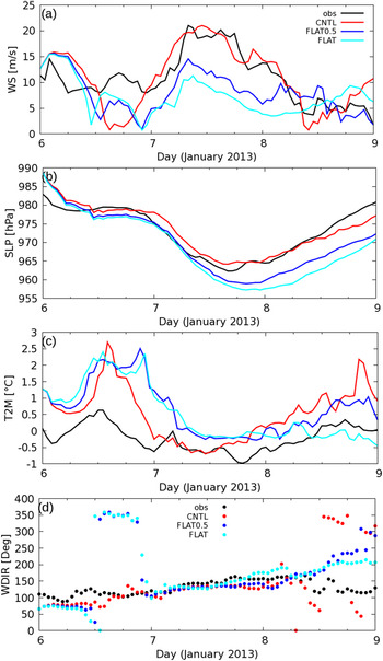
The temporal evolution of meteorological variables reproduced by the three experiments is compared with observations in Fig. 2. The observed wind speed at KSJ was ~8.6 m/s at 00h00 UTC on 7 January and rapidly increased to reach its maximum value of ~21 m/s at 08h00 UTC; it remained at this wind speed until 18h00 UTC. The CNTL experiment successfully represented the strong wind in terms of its peak speed with an accuracy of ~94% (~19.7 m/s), whereas the FLAT experiment significantly underestimated the peak wind speed by ~51% (~10.4m/s). FLAT0.5 also underestimated the peak wind speed, but showed a better result, with a value of ~14 m/s (69.5% of the observation), than the FLAT experiment. This result suggests that the topography effect accounted for ~50% of the factors producing the strong wind at KSJ in this case study.
Time series of hourly mean a. 10 m wind speed (m/s; WS), b. sea-level pressure (hPa; SLP), c. 2 m temperature (°C; T2M) and d. wind direction (°; WDIR) from observations and the Polar Weather Research and Forecasting experiments (3 km) using the CNTL, FLAT0.5 and FLAT configurations.

Sea-level pressures simulated from the three experiments generally agree with observations before the occurrence of the maximum wind speed (Fig. 2b). However, sea-level pressures from FLAT0.5 and FLAT started to diverge from observed values at ~08h00 UTC on 7 January, and the differences between the simulation and observations became gradually larger with time. FLAT0.5 and FLAT showed much lower sea-level pressures than the observations. The sea-level pressure reproduced by the CNTL experiment is in good agreement with observations for most of the time period studied. The 2 m temperature from three model experiments showed relative distinctions from the observations compared to other variables. In general, three experiments were able to capture the temporal variation of the 2 m temperature, but they tended to overestimate the 2 m temperatures compared to observations, especially prior to 07h00 UTC on 7 January. A decrease of the 2 m temperature during the high wind speed event is explained by cold advection from the Weddell Sea and the AP to KSJ caused by the strong south-easterly over the AP, as reported in Kwon et al. (Reference Kwon, Park, Lee, Kim, Choi and Kim2019). The CNTL experiment reproduced a decrease of the 2 m temperature during high winds, similar to the observations. In contrast, the FLAT0.5 and FLAT results showed a large difference in the 2 m temperature during high winds. This shows that a failure to properly represent a strong south-easterly caused by strong deformation of the sea-level pressure fields around the AP in FLAT0.5 and FLAT leads to a misrepresentation of variation in the 2 m temperatures during the strong wind phase.
The three experiments produced good representations of the south-easterly (110°–150°) for the high wind period on 7 January shown in Fig. 2d. On the other hand, all of the experiments resulted in significant differences from the observed wind direction between 6 and 8 January.
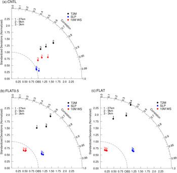
Figure 3 shows the models' abilities to simulate 10 m wind speed, sea-level pressure and 2 m temperature with different horizontal grid resolutions from the three experiments. Simulation ability for the strong wind event is highly dependent on horizontal resolution in the CNTL experiment. The 3 km simulation results showed the best agreement with observations for all selected variables. On the other hand, the simulation results from the FLAT0.5 and FLAT experiments showed relatively little sensitive to the horizontal resolution, except for the 2 m temperature. As the topography of the AP in CNTL is higher than that in FLAT0.5 and FLAT, the representation of topography in CNTL is more sensitive to horizontal resolution than the other two experiments. Therefore, the CNTL experiment shows a large difference in the simulation results of the strong wind event affected by AP topography depending on horizontal resolution. This suggests the importance of high-resolution model domains in simulating strong wind events, especially when the event is strongly influenced by local topography.
Taylor diagrams for the 10 m wind speed (red circles; WS), sea-level pressure (blue circles; SLP) and 2 m temperature (black circles; T2M) at horizontal grid resolutions of 27 (number 1), 9 (number 2) and 3 km (number 3) relative to observations. a., b. and c. show the results for the CNTL, FLAT0.5 and FLAT experiments, respectively.

Sensitivity of strong wind simulation to terrain height
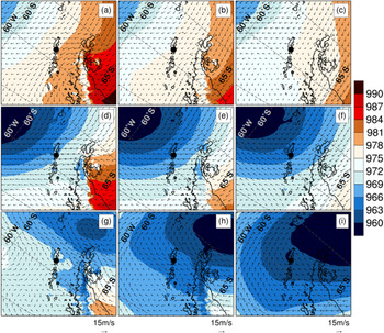
Figure 4 shows the large-scale features of sea-level pressure and wind field from the CNTL (Fig. 4a & d), FLAT0.5 (Fig. 4b & e) and FLAT (Fig. 4c & f) experiments with a 3 km horizontal resolution at the onset (00h00 UTC on 7 January) and during the peak (08h00 UTC on 7 January) phase of the strong wind event. In CNTL, one edge of the cyclone spanned towards King George Island at the onset (Fig. 4a). The low-pressure system then moved south-eastwards with time, producing a decrease in sea-level pressure and increasing the wind speed over KSJ during the strongest phase of the wind event (Fig. 4d). At this stage, the isobar interval around KSJ was much narrower than at the onset stage. Note that as the low-pressure system approached the AP, the isobars around the AP became deformed because of the topography. The large isobar discontinuity was noted around the eastern coastline of the AP at 00h00 UTC on 7 January (Fig. 4a), becoming stronger at 08h00 UTC on 7 January (Fig. 4d).
Sea-level pressure (shading, 2 hPa intervals) and wind vectors (arrows) at 00h00 UTC on 7 January 2013 (first row), 08h00 UTC on 7 January 2013 (second row) and 09h00 UTC on 8 January 2013 (third row) from the 3 km Polar Weather Research and Forecasting simulations of the CNTL (a., d. and g.), FLAT0.5 (b., e. and h.) and FLAT (c., f. and i.) experiments. King Sejong Station is represented by filled black circles.

The FLAT0.5 and FLAT experiments represent different wind and sea-level pressure fields from CNTL (Fig. 4b, c, e & f). The most pronounced difference from the CNTL experiment was the distribution of the sea-level pressure around the east coast of the AP throughout the whole period (Fig. 4k & l). FLAT0.5 produced an isobar discontinuity around the eastern coastline of the AP at 00h00 UTC and 08h00 UTC on 7 January, but this was weaker than in the CNTL results. The FLAT simulation, however, did not produce a deformation of the isobar field around the east of the AP (Fig. 4f). This comparison clearly shows that the topography of the AP leads to strong deformation of the sea-level pressure pattern as the low-pressure system approaches. Note that the wind field was also significantly different between the three experiments, consistent with sea-level pressure differences. Both the intensity and the position of the cyclone centre were similar at the beginning stage of the three experiments, but their differences became gradually more pronounced with time. During the cessation phase at 09h00 UTC on 8 January, the wind became weaker at KSJ and the low-pressure system moved further south-east (Fig. 4g–i).
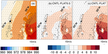
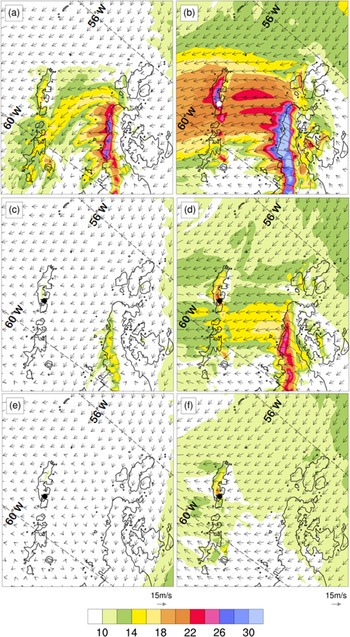
Differences in wind field around KSJ in the three experiments are shown in the enlarged view (Fig. 5). The largest difference in the wind fields of the three experiments was noted on the downwind side around the west coast of the AP and King Gorge Island, where KSJ is located. The original terrain of the AP (CNTL) causes the formation of weak easterly (~100°) winds across the mountain barrier on the eastern coast at the onset due to strong isobar deformation (Fig. 5a). The enhanced pressure gradient around the east coastline of the AP generates east-south-easterly winds across the mountain barrier. This flow speeds up over time and turns into a strong south-easterly flow (~130°). It induces a strong downslope wind at the leeward side (western side from the ridge) of the AP with a distinct wind direction difference from surrounding areas (Fig. 5b). A region of high wind speed is observed along the western side of the AP. Kwon et al. (Reference Kwon, Park, Lee, Kim, Choi and Kim2019) showed that this downslope windstorm plays an important role in further intensifying the wind at KSJ. They concluded that the strong wind event was induced by a joint effect of an approaching cyclone together with the local topographical characteristics.
An enlarged view of sea-level pressure (shading) and wind vectors (arrows) around King Sejong Station (KSJ) at 00h00 UTC on 7 January 2013 for climatology (a.) and the difference between the CNTL and FLAT0.5 and the CNTL and FLAT experiments (b. and c., respectively). Shading intervals in the difference map are 2 hPa. KSJ is represented by filled black circles.

Considering a terrain height reduced by 50% (FLAT0.5), the east-south-easterly wind across the AP was formed during the onset and mature phases, but with a much weaker intensity than in CNTL (Fig. 5c & d). On the other hand, the FLAT experiment did not reproduce the south-easterly wind across the AP during the onset and mature phases (Fig. 5e & f). In contrast to the CNTL results, weak north-easterly and easterly winds prevailed over the AP at 00h00 UTC and 08h00 UTC on 7 January, respectively, and the downslope windstorm driven by south-easterly flow was not properly represented due to the absence of the AP topography. As a result, the high wind region along the western side of the AP shown in CNTL was not generated in the FLAT experiment. In FLAT0.5, a strong wind appears along the western side of the AP, but its strength is ~31% weaker than in CNTL. Consequently, the strong wind at 08h00 UTC on 7 January was not properly reproduced at KSJ in either FLAT0.5 or FLAT. This clearly indicates that the topography of the AP had a critical influence on the occurrence of strong winds on 7 January at KSJ.
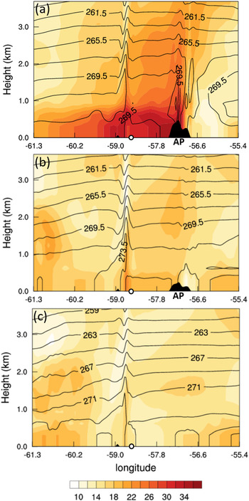
The effect of AP topography is more clearly seen in the vertical section of the horizontal wind and potential temperature. Figure 6 shows a vertical cross-section of the horizontal wind and potential temperature from point A to point B (Fig. 1b) during the strongest wind speed phase (08h00 UTC on 7 January). Both the wavy structure of the potential temperature over the AP and high wind speeds on the western side of the AP were shown in CNTL (Fig. 6a); furthermore, this clearly shows the characteristics of the downslope windstorm. FLAT0.5 produced a weaker wavy structure of potential temperature over the AP and wind speeds on the western side of the AP that were ~16 m/s weaker than the CNTL result. On the other hand, neither the structure of the potential temperature over the AP nor the high wind speed region on the western side of the AP was produced in the FLAT experiment.
Wind speed (shading, 2 m/s intervals) and wind vectors (arrows) for an enlarged region over King Sejong Station (KSJ) at 00h00 UTC and 08h00 UTC on 7 January 2013 from the 3 km Polar Weather Research and Forecasting simulation of CNTL (a. and b., first row; Kwon et al., Reference Kwon, Park, Lee, Kim, Choi and Kim2019), FLAT0.5 (c. and d., second row) and FLAT (e. and f., third row). KSJ is represented by filled black circles.

The Froude number (Fr) can be used to determine whether an atmospheric flow could override a mountain barrier or be deflected around it. The Fr used in this study is:
 $${\rm Fr} = U_0\left({{\rm g}H\displaystyle{{\Delta {\rm \theta }} \over {\rm \theta }}} \right)^{{-}1/2}, \;$$
where U 0 is the wind speed, g is the gravitational acceleration (9.8 m/s2), H is the height of the obstacle, △θ is the increase in potential temperature of the layer between the surface and the top of the obstacle and θ is the average potential temperature of the layer between the surface and the height of the obstacle (O'Connor & Bromwich Reference O'Connor and Bromwich1988). The Fr is derived from the model output at a point (-56.82°E, -63.6°S) on the x-axis (longitude) of Fig. 7a. The values used to calculate the Fr are described in Table I. In CNTL, the Fr substantially increased from 1.8 at 00h00 UTC to 3.7 at 08h00 UTC on 7 January at the windward side of the AP. Fr > 1 indicates that the atmospheric flow has sufficient kinetic energy to override the topographical barrier. A continuous flow overriding the AP topography, under conditions of Fr > 1, is crucial for the generation of the downslope windstorm. FLAT0.5 also resulted in Fr > 1 (1.2 at 00h00 UTC and 2.3 at 08h00 UTC on 7 January), but its value is smaller than that in CNTL.
Vertical cross-section of the potential temperature (contour, 2 K intervals) and horizontal wind speed (shading, 2 m/s intervals) along the line from point A (left corner on x-axis) to point B (right corner on x-axis) shown in Fig. 1b at 08h00 UTC on 7 January 2013 for a. CNTL, b. FLAT0.5 and c. FLAT. White circles represent the location of King Sejong Station. AP = Antarctic Peninsula.

The Froude numbers (Fr) and representative values of model outputs used for the Fr calculations at 00h00 UTC and 08h00 UTC on 7 January 2013.

H = topographical height, U 0 = mean wind speed; θ = potential temperature.
Summary and conclusion
In this study, we investigated the effects of AP topography on a strong wind event that occurred on 7 January 2013 at KSJ, Antarctica. A series of numerical experiments using three different terrain heights was conducted using Polar WRF to quantitatively estimate the effect of AP topography on driving the strong wind event. Using simulations of 100% (CNTL), 50% (FLAT0.5) and 0% (FLAT) of the terrain heights of the AP, we examined the sensitivity of the wind speed to the different terrain heights.
The simulation ability for strong wind events appears to be sensitive to horizontal resolution in the CNTL experiment. The highest horizontal resolution (3 km) best reproduces the observed wind speed, sea-level pressure and 2 m temperature. In contrast, the FLAT0.5 and FLAT experiments showed a relatively low sensitivity of simulation ability to horizontal resolution compared to the CNTL experiment, except for in the 2 m temperature. This is due to the small difference in terrain height depending on the horizontal resolution in the FLAT0.5 and FLAT experiments when we use the relatively low terrain height of the AP. This supports the importance of high-resolution model domains when reproducing strong winds affected by local topography.
The numerical simulation of the strong wind event using the original AP topography (CNTL) successfully reproduced the features of the strong wind, both in terms of the strength and the sharp change of the speed. It well captured the peak wind at KSJ (~19.7 m/s, ~94% of the observed value). In contrast, the numerical simulation using flattened terrain (FLAT) significantly underestimated peak wind speeds by ~51% (~10.4 m/s of the observed value). The FLAT0.5 experiment also underestimated peak wind speeds but showed better results than the FLAT experiment, producing a value of ~14 m/s (69.5% of the observed value), indicating the significant influence of upstream topographical effects. In addition, these numerical experiments also demonstrated that the absence of AP topography leads to a failure to simulate the strong discontinuity of the sea-level pressure fields around the eastern coast of the AP, which is an important condition for a continuous south-easterly overriding the AP. As a result, without topography, the downslope windstorm driven by a flow overriding the AP is not formed on the western side of the AP, resulting in no further enhancement of the wind speed at KSJ located on the western side of the AP. The simulation results for sea-level pressure, 2 m temperature and wind direction at KSJ from both the FLAT and FLAT0.5 experiments showed less agreement with the observations than the results of the CNTL experiment.
In conclusion, the effect of topography along the AP played a critical role in the occurrence of the strong wind event at KSJ on 7 January 2013, accounting for ~50% of the total wind speed. There are several previous studies that have highlighted the influence of topography on strong wind events over Antarctica (Steinhoff et al. Reference Steinhoff, Bromwich, Lambertson, Knuth and Lazzara2008, Nigro et al. Reference Nigro, Cassano, Lazzara and Keller2012, Orr et al. Reference Orr, Phillips, Webster, Elvidge, Weeks, Hosking and Turner2014, Chenoli et al. Reference Chenoli, Turner and Samah2015). Whereas previous studies mainly analysed the indirect influence of topography through weather analysis, this study quantitatively evaluated the effect of the complex topography of the AP on the occurrence of a strong wind through a series of direct numerical sensitivity experiments. Our study implies that, for better prediction of strong wind events over AP regions, we need to consider not only the correct simulation of cyclones, but also the interaction between the adjacent topography and wind induced by such cyclones.
Note, however, that only one strong wind event at KSJ was investigated in this study. Therefore, more case studies are required in order to generalize the effect of AP topography on the occurrence of strong wind at KSJ.
Financial support
This work was supported by the National Research Foundation of Korea (NRF) grant funded by the Korea government (NRF-2020R1A2C1014679) and the Korea Polar Research Institute research project (PE21030).
Author contributions
HK and S-JK designed the research, conducted the analyses and wrote the main part of the manuscript. S-WK was involved in discussing the results and wrote the manuscript. SK contributed to the Polar WRF model simulation.
Data availability
The model output is available on request from the corresponding author. The ERA-Interim analysis data were obtained from the ECMWF data server (https://apps.ecmwf.int/datasets/data/interim-full-daily/levtype=sfc/). The AMOS data at KSJ are available on request from the corresponding author.