Introduction
The Drake equation (Drake Reference Drake1962) provides a truly helpful educated guess, a rational set of lenses – the factors in the equation – through which to look at future contacts with technologically advanced civilizations in the Milky Way. The equation quantifies the number of civilizations from whom we might receive an electromagnetic signal, using a collection of factors that have been extensively discussed in the literature and whose estimated values are revised continually. A comprehensive review and an analysis of each term of the equation are presented in Vakoch and Dowd (Reference Vakoch and Dowd2015). Optimistic estimates from the Drake equation contrast with the so-called Fermi paradox, which states the apparent contradiction between the expected abundance of life in the Galaxy and the lack of evidence for it (e.g. Hart Reference Hart1975; Brin Reference Brin1983; Barlow Reference Barlow2013; Anchordoqui et al. Reference Anchordoqui, Weber and Fernandez Soriano2017; Forgan Reference Forgan2017; Carroll-Nellenback et al. Reference Carroll-Nellenback, Frank, Wright and Scharf2019; Sotos Reference Sotos2019). There are many propositions aimed at solving this paradox, which make use of statistical (Horvat Reference Horvat2006; Maccone Reference Maccone2015; Solomonides et al. Reference Solomonides, Kaltenegger and Terzian2016) or stochastic approaches (Forgan Reference Forgan2009; Forgan and Rice Reference Forgan and Rice2010; Glade et al. Reference Glade, Ballet and Bastien2012; Bloetscher Reference Bloetscher2019). Regarding the Drake equation, analytical interpretations (Prantzos Reference Prantzos2013; Smith Reference Smith2009) or reformulations (Burchell Reference Burchell2006, and references therein) have also been proposed. The absence of detections of extraterrestrial intelligent signals could be explained by astrophysical phenomena that makes life difficult to develop (Annis Reference Annis1999). Besides the possible scarcity of life, alternative scenarios have also been discussed (Barlow Reference Barlow2013; Lampton Reference Lampton2013; Forgan Reference Forgan2017; Conway Morris Reference Morris2018). The large distances in the Galaxy and the likely limited lifetime of civilizations may play an important role in determining how difficult it would be to obtain evidence for other inhabited worlds. The analysis of these scenarios is difficult due to the lack of data about the hypothetical extraterrestrial intelligences. Indeed, as Tarter (Reference Tarter2001) pointed out, according to our current technical capabilities for the search of extraterrestrial intelligence (SETI), we have not received any signal yet. The absence of detections has also motivated alternative ideas for new SETI strategies (Loeb and Zaldarriaga Reference Loeb and Zaldarriaga2007; Tarter et al. Reference Tarter, Backus, Blair, Cordes, Harp, Henry, Horowitz, Howard, Kilsdonk, Korpela, Lasio, Levin, Shostack and Werthimer2009; Maccone Reference Maccone2010, Reference Maccone2011a; Forgan Reference Forgan2013; Maccone Reference Maccone2013, Reference Maccone2014b; Wright et al. Reference Wright, Cartier, Zhao, Jontof-Hutter and Ford2015; Loeb et al. Reference Loeb, Batista and Sloan2016; Enriquez et al. Reference Enriquez, Siemion, Foster, Gajjar, Hellbourg, Hickish, Isaacson, Price, Croft, DeBoer, Lebofsky, MacMahon and Werthimer2017; Forgan Reference Forgan2017; Balbi Reference Balbi2018a; Harp et al. Reference Harp, Ackermann, Astorga, Arbunich, Barrios, Hightower, Meitzner, Barott, Nolan, Messerschmitt, Vakoch, Shostak and Tarter2018; Lingam and Loeb Reference Lingam and Loeb2018; Forgan Reference Forgan2019; Funes et al. Reference Funes, Florio, Lares and Asla2019).
The discussion about the problem of the unknown abundance of civilizations in the Galaxy has been organized around the factors in the Drake equation (Hinkel et al. Reference Hinkel, Hartnett, Lisse and Young2019). However, the uncertainties in these factors, specially the ones representing biological processes, make it less suitable to a formal study with the purpose of defining searching strategies or computing the estimated number of extraterrestrial intelligences. A number of studies propose alternative formalisms for the estimation of the likelihood of detecting intelligent signals from space. Prantzos (Reference Prantzos2013), for example, proposes a unified framework for a joint analysis of the Drake equation and the Fermi paradox, concluding that for sufficiently long-lived civilizations, colonization is the most promising strategy to find other life forms. Haqq-Misra and Kopparapu (Reference Haqq-Misra and Kopparapu2018) discuss the dependence of the Drake equation parameters on the spectral type of the host stars and the time since the Galaxy formed, and examine trajectories for the emergence of communicative civilizations. Some modifications to the original idea of the Drake equation have been proposed, in order to integrate a temporal structure, to reformulate it as a stochastic process or to propose alternative probabilistic expressions. Temporal aspects of the distribution of communicating civilizations and their contacts have been explored by several authors (Fogg Reference Fogg1987; Forgan Reference Forgan2011; Horvat et al. Reference Horvat, Nakić and Otočan2011; Balbi Reference Balbi2018a, Reference Balbi2018b), as well as efforts on considering the stochastic nature of the Drake equation (Glade et al. Reference Glade, Ballet and Bastien2012).
Several authors raise the distinction between causal contacts and actual contacts. In the first case, the determinations of metrics for the likelihood of a contact are independent of considerations about the technological resources or the implicit coordination to decipher intelligent messages. In a recent work, Balbi (Reference Balbi2018a) uses a statistical model to analyse the occurrence of causal contacts between civilizations in the Galaxy. The author highlights the effect of evolutionary processes when attempting to estimate the number of communicating civilizations that might be in causal contact with an observer on the Earth. Ćirković (Reference Ćirković2004) also emphasizes the lack of temporal structure in the Drake equation and, in particular, the limitations of this expression to estimate the required timescale of a SETI program to succeed in the detection of intelligent signals. Balbi (Reference Balbi2018a) also investigates the chance of communicating civilizations making causal contact within a volume surrounding the location of the Earth. The author argues that the causal contact requirement involves mainly the distance between civilizations, their lifespan and their times of appearance. This is important since the time the light takes to travel across the Galaxy might be much lesser than the lifetime of the emitter. Balbi (Reference Balbi2018a) fixes the total number of civilizations and explores the parametric space that comprises three variables, namely, the distance to the Earth, the time of appearance and the lifespan of the communicating civilizations. Each of these three variables are drawn from a random distribution. The distances are drawn from a uniform model for the positions of civilizations within the plane of the Galaxy. For the distribution of the characteristic time of appearance, the author explores exponential and truncated Gaussian functions, while for the lifespans chooses an exponential behaviour. It is important to point out that the estimation of the number of communicating civilizations varies with the choice of the statistical model for the time of appearance, as shown by Balbi (Reference Balbi2018a). For all analysed distributions, the author concludes that the fraction of emitters that are listened is low if they are spreaded in time and with limited lifetimes. An analytical explanation of these concepts is presented in Grimaldi (Reference Grimaldi2017), who considers a statistical model for the probability of the Earth contacting other intelligent civilizations, taking into account the finite lifetime of signal emitters, and based on the fractional volume occupied by all signals reaching our planet.
The quest for a formal statistical theory has also lead to important progress in the mathematical foundations of SETI. Recently, Bloetscher (Reference Bloetscher2019) considers a Bayesian approach, still motivated by the Drake equation, to estimate the number of civilizations in the Galaxy. To that end, the authors employ Monte Carlo Markov Chains over each factor of the Drake equation, and combine the mean values to reach a probabilistic result. It is worth mentioning that the author proposes a log-normal target distribution to compute the posterior probabilities. This study concludes that there is a small probability that the Galaxy is populated with a large number of communicating civilizations. Smith (Reference Smith2009) uses an analytical model to gauge the probabilities of contact between two randomly located civilizations and the waiting time for the first contact. The author stresses that the maximum broadcasting distance and the lifetime of civilizations come into play to produce the possible network of connections.
On this topic a number of works consider numerical simulations (Forgan Reference Forgan2009, Reference Forgan2017; Murante et al. Reference Murante, Moncaco, Borgani, Tornatore, Dolag and Goz2015; Forgan et al. Reference Forgan, Dayal, Cockell and Libeskind2016; Vukotić et al. Reference Vukotić, Steinhauser, Martinez-Aviles, Ćirković, Micic and Schindler2016; Ramirez et al. Reference Ramirez, Gómez-Muñoz, Vázquez and Núñez2017). Although this approach does not rely on values that can be measured from observations (like the fraction of stars with planets), it depends on the definition of unknown or uncertain parameters required to carry out the simulations. In another numerical approach, Vukotić and Ćirković (Reference Vukotić and Ćirković2012) propose a probabilistic cellular automata modelling. In this framework, a complex system is modelled by a lattice of cells which evolve at discrete time steps, according to transition rules that take into account the neighbour cells. The authors implement this model to a network of cells which represent life complexity on a two-dimensional region resembling the Galactic Habitable Zone (GHZ), an annular ring set between a minimal radius of 6 kpc and a peak radius of 10 kpc. These simulations represent the spread of intelligence as an implementation of panspermia theories. Within this framework, Vukotić and Ćirković (Reference Vukotić and Ćirković2012) also make Monte Carlo simulations and analyse ensemble-averaged results. Their work aims at analysing the evolution of life, and although it does not account for the network of causal contacts among technological civilizations, it offers a tool to think SETI from a novel point of view.
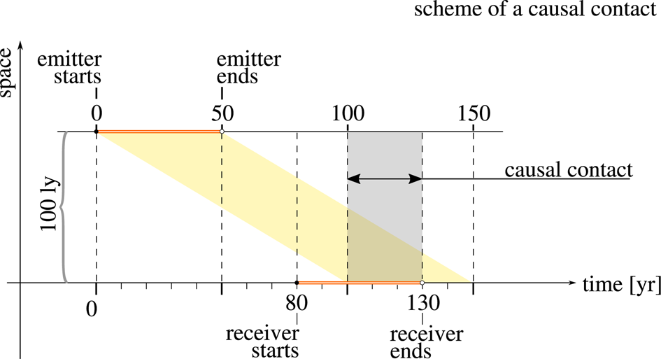
This study is conceived as an introduction to a simple probabilistic model and a numerical exploration of its parameter space. With these tools, we address the problem of the temporal and spatial structure of the distribution of communicating civilizations. This approach does not require assumptions about, e.g., the origin of life, the development of intelligence or the formation of habitable planets according to stellar type. Instead, we assume monoparametric function families to model the appearance of points in the disk of the Galaxy and over the time, which we call nodes. These nodes represent the locations of ideal intelligent agents that are able to receive and emit signals with perfect efficiency in all directions. Then we analyse the network of causally connected nodes limited to have a maximum separation representing the maximum distance a signal can travel with an intensity above a fixed threshold. A node is causally connected to other nodes if it is within their light cone. We adopt as a definition that a light cone is the region in spacetime within the surface generated by the light emanating from a given point in space in a given period of time. For example, two nodes separated by 100 light years, which appear with a difference in time of 80 years and last 50 years each, will be causally connected for 30 years. This connection is not, though, bidirectional. In fact, the second node will see the first one for 30 years, but the first node will never acknowledge the existence of the second. A scheme of this example is shown if Fig. 1. This simple taught experiment exemplifies the importance of the time variable to analyse the structure of connections. The model can be described with three parameters, namely, the mean separation between the appearance of nodes, the mean lifetime of the nodes and the maximum separation to allow an effective causal contact. The model presented here comprises the stochastic networks of constrained causally connected nodes, together with the three parameters and additional hypotheses. Hereafter, we refer to this model as the SC3Net model, standing for ‘Stochastic Constrained Causally Connected Network’.
Example of a configuration of an emitter and a receiver to produce a causal contact. The observers are separated by 100 light years and appear with a difference in time of 80 years. One observer is active between t = 0 and t =50 years. The other observer is also active for 50 years, between t =80 and t =130 years. The causal connection occurs between t =100 and t =130 years. Meaningful times are marked with vertical dashed lines.

We provide a framework to explore, through a suite of numerical simulations, the parameter space of three unknown observables. This allows to discuss possible scenarios and their consequences in terms of the probability of making contacts. The method we use for simulating a stochastic process is an approximation that allows to study the behaviour of complex systems, by considering a sequence of well-defined discrete events. The simulation is carried out by following all the variables that describe and constitute the state of the system. The evolution of the process is then described as the set of changes in those variables. In this context, an event produces a specific change in the state that can be triggered by random variables that encode the stochastic nature of the physical phenomenon. For example, when a new contact is produced between two entities in the simulated galaxy, the number of active communication lines is increased by one. Also, if it is the first contact for that nodes, then the number of communicated nodes increases by two. When a new node becomes active, the system has an increase of one in the number of nodes, although the number of communications does not necessarily change. The process then involves following the changes on the state of the system, defining the initial and final states. This is done by defining a method that allows to keep track of the time progress in steps and maintaining a list of relevant events, i.e., the events that produce a change in the variables of interest. With this method we abandon the frequentist approach of the Drake equation to compute the number of civilizations, providing instead its statistical distribution. More importantly, we are interested in the probability of contacts, which depend critically on the time variable. This is an exploratory analysis that aims at developing a numerical tool to discuss the different scenarios based on statistical heuristics. The approach proposed here should be considered as a compromise between the uncertainties of the frequentist estimations and the detailed recipes required on the numerical simulations. It is worth noticing that the SC3Net model is not intended for a formal fit at this stage due to the lack of data, but it can help to understand how unusual it would be to actively search for intelligent signals for 50 years without positive detections.
This paper is organized as follows. In section ‘Methods and working hypotheses’ we introduce the methods and discuss the candidate distributions for the statistical aspects of the times involved in the communication process. We present our results in section ‘Results: exploring the parameter space’, with special emphasis on the statistical distributions of the duration of causal contacts in and the distribution of time intervals of waiting for the first contact. These quantities are considered as a function of the three simulation parameters. In section‘Discussion’ we discuss our results and future research directions.
Methods and working hypotheses
Simulations are suitable tools to analyse systems that evolve with time and involve randomness. An advantage of a numerical approach is that it usually requires fewer assumptions and simplifications, and can be applied to systems where analytical models are hard or impossible to develop. In particular, a suitable tool to model complex stochastic processes through the changes in the state of a system is the discrete-event (hereafter, DE) simulation approach. A system described with the DE paradigm is characterized by a set of actors and events. Actors interact causally through a series of events on a timeline and process them in chronological order (Chung Reference Chung2003; Ross Reference Ross2012; Ptolemaeus Reference Ptolemaeus2014). Each event modifies the variables that define the process, producing the corresponding change in the state of the simulated system. This method is well suited for the particular case of the diffusion of intelligent signals in the Galaxy and allows to explore several models easily. We simulate the statistical properties of a set of points in space and time that have a causal connection at light speed and are separated by a maximum distance. We refer to these nodes as ‘Constrained Causal Contact Nodes’ (hereafter, node). We choose this generic name in order to stress the fact that in this analysis only the causal contact is considered, independently of any broadcasting or lookout activity. The system we propose is ideal, in the sense that it considers the special case of a fully efficient node that emits and receives isotropically. A causal contact node, considered as a broadcasting station that has the ability to detect signals through an active search program, could have a lesser than one efficiency factor, which is not included in the current analysis. Also, it is worth mentioning that this is a general approach, and not necessarily a node is the host of an intelligent civilization. It can be associated with a planet where life has developed, became intelligent, reached the skills required to find the right communication channel, sustained a search and established a contact. Alternative message processing entities could be considered, for example, interstellar beacons where intelligent life has ceased to exist but continue with its emission, or communication stations established by probes or left by intelligent beings (see, e.g., Barlow Reference Barlow2013; Peters Reference Peters2018). In principle, these strategies could affect our results since it would be easier to configure a cluster of nodes that spread in time. However, we do not consider these speculative alternatives at this point. For the purpose of the present analysis, only the communication capability is relevant, since we study the causal contacts between the locations. The system is defined by a number of actors that represent nodes and appear at different instants in time, generating events that produce meaningful changes in the variables that describe the system, i.e., in the arrangement of nodes and their network of causal contacts. For example, the appearance of a new node in a region filled with a signal emitted by another node will increase the number of active nodes and the number of pairs of nodes in causal contact. Assuming some simple hypotheses, the discrete events method can be performed taking into account a small number of variables, which allow to analyse the variation of the results in the SC3Net model parameter space.
In what follows, we outline the experimental setup adopted to estimate the probabilities of causal contacts and several derived quantities. This is done in terms of three independent parameters, namely, the mean time span between the appearance of consecutive nodes, τa, their mean lifetime τs, and the maximum distance a signal can be detected by another node (D max). Intuitively, the probability of the existence of causal contacts between pairs of nodes would be larger for smaller τa parameters, higher τs or higher D max parameter values. We also propose theoretical distribution functions for both the lifespans (τs) and the number of nodes per unit time (Maccone Reference Maccone2014a; Sotos Reference Sotos2019). The latter is related to the time span between the appearance of consecutive nodes (since when τa is shorter, it produces a greater density of nodes). The analytical expressions for these distributions are set to a fixed law, as discussed in section‘Power laws versus exponential laws’.
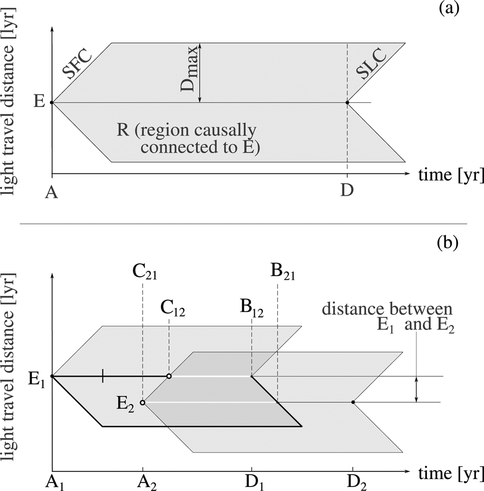
Space–time diagrams, where time and space are represented on the horizontal and vertical axes, respectively, are suitable tools to describe the causal connections among different nodes. We illustrate in Fig. 2 the schematic representation of the region causally connected to a given node. For the sake of simplicity, we show in the plot the light travel distance, i.e., the distance traversed by any signal spreading from the emitter at light speed (e.g., any electromagnetic signal). In this scheme, a light pulse would follow a trajectory represented by a line at 45 degrees from the axes, given the units of time and space axes are years and light years, respectively. Panel (a) represents the region R (shaded polygon) which is causally connected to the emitter (left vertex). This region develops after an event (hereafter dubbed A-type event) in which the node acquires the communication capability, or becomes ‘active’. The sphere of first contact (SFC) is centred on the emitter, represented by the left angle of the region R. This sphere grows until its radius reaches the D max distance, in which it would be no longer detectable due to the decrease in the energy per unit area, which falls under the assumed detectability threshold. Similarly, the surface of last contact (SLC) is another sphere that grows from an event in which the nodes cease to possess the communication capability (D type event), and carries the last signal produced by the emitter. The region which is causally connected to the emitter is then limited by these two spheres and therefore has the shape of a filled sphere (before the D event) or of a spherical shell (after the D event). The temporal intervals for the communication between two nodes are represented in panel (b) of Fig. 2. In this scheme, the entire lifetime of a node can be represented by a polygon. This polygon is limited in the spatial axis by the maximum distance of the signal D max and in the time axis by the time span between the A-type event (concave vertex) and the D-type event (convex vertex). This representation allows to visualize the important events that result from the presence and communications of two nodes. The points in time where the nodes acquire their communicating capacity are dubbed ‘Awakening’ events (A1 and A2). Similarly, the instants in time where the nodes lose their communicating capacity are dubbed ‘Doomsday’ events (D1 and D2). The points in space–time where the first contact is produced for each one of the nodes are defined as ‘Contact’ events, shown as C1 and C2. Finally, the two points where the contact is lost for each one of the nodes are denominated ‘Blackout’ events, presented as B1 and B2. The receiver node E1 can listen to signals from the emitter node E2, from the first contact event (t = C12) until the last one (t = B12). Similarly, the receiver node E2 can listen to signals from the emitter node E1, from t = C21 up to t = B21. The time intervals for the open communication channel are determined by the ‘C’ and ‘B’ type events. It is noteworthy of the fact that there is a time delay between the contact events of the two nodes involved in this analysis, and also a time delay between the two blackout events. Therefore, the time range when a bidirectional contact is possible occurs between the maximum time of the contact points and the minimum time between the blackout points.
Space–time diagrams showing a schematic representation of the different stages in the development of a constrained causal contact node. Panel (a) represents the region R in space and time which is causally connected to the emitter (E, left vertex), following an ‘A’ type event (‘Awakening’) in which the node acquires the communication capability. The sphere of the first contact (SFC) is the sphere centred on the emitter that grows until its radius reaches the D max distance, in which the power of the signal would equal the detectability threshold. This sphere is represented by the left triangle of the region R. The surface of the last contact (SLC) is another sphere that grows from a ‘D’ event (‘Doomsday’). The region which is causally connected to the emitter is then limited by these two spheres, and has the shape of a sphere or of a spherical shell, depending on the time. The temporal intervals for the communication between two nodes are represented in panel (b). The node E1 can listen to signals from the node E2, since the ‘Contact’ event (t = C12) up to the ‘Blackout’ event (t = B12). Similarly, the node E2 is in causal contact from the node E1, in the time interval (C21, B21).

The temporal structure that emerges from the experimental setup implies that, as a fundamental property of the simulations, a causal connection can be produced without requiring that the two nodes are active at the same time. This property of the system arises as a consequence of the large spatial and temporal scales, where a message is transmitted at the (relatively small) light speed. Although a node could be active for a large enough period to transmit a message at large distances, the limited power of the message and the dilution that depends on the squared distance from the source imposes a detectability limit. As a consequence of this limitation and of their finite lifetime, considered as the period between the acquisition and loss of communicating capacity, each node will fill a spherical shell region of the Galaxy, limited by two concentric spherical surfaces. The leading front, or surface of first contact (SFC) grows from the central node until it reaches the maximum distance D max. Following the end of the civilization, there is still a region which is filled with the emitted signals. This approach has been also considered in other statistical models (e.g., Smith Reference Smith2009; Grimaldi Reference Grimaldi2017; Grimaldi et al. Reference Grimaldi, Marcy, Tellis and Drake2018). The trailing front, or surface of last contact (SLC) also grows from the central node, with a delay with respect to the SFC equivalent to the lifetime of the node, and produces a spherical shell region. Any other node within this region will be in causal contact with the originating node, even if it has disappeared before the time of contact. This region will grow if the surface of first contact has not yet reached the maximum distance D max, and will shrink after a D-type event until the surface of last contact reaches D max, producing as a result the loss of all signal from the central node. In our approach, we consider a model galaxy where the width of the disk is negligible with respect to the radius of the disk. In the 2D simulation only the intersection of the communicating spherical shells with the plane of the Galaxy is relevant, and produce the corresponding circles or rings for the filled spheres or annular regions of the spherical shells, respectively. The initially growing communicating sphere is shown over space–time diagrams, where time is represented on the horizontal direction, and space is represented in the vertical direction. In Fig. 2 the two emitters in panel (b), E1 and E2, reach each other at different times. The time span for Ei is (A i, D i), for i = 1, 2. Emitter i can listen to emitter j between C ij and B ij. The type and length of causal contact in both directions depend on the distance and time lag between the awakening events, the maximum distance that a signal can reach and the time period in which each emitter is active.
In our experimental configuration the simulation starts assuming that the stochastic process is already stable, and finishes before any galactic evolution effect could modify the fixed values of the variables. Likewise, we assume that the probability for the appearance of a node is homogeneous over the GHZ. The adopted geometry of the GHZ in all the simulations is given by a two-dimensional annular region, with an inner radius of 7 kpc and an outer radius of 9 kpc (Lineweaver et al. Reference Lineweaver, Fenner and Gibson2004). Although the Galaxy has a well-known spiral structure, the nodes are assumed to be sparse (otherwise the Galaxy would be full of life) and the spiral structure would not, in that case, produce significant differences. If the distribution of nodes is not sparse, as it could be the case if the spiral arms host most of the nodes, then contacts would be more frequent between closely located nodes. In such a case our results underestimate the number of contacts between close pairs of nodes within the same spiral arm, and conversely, overestimate the number of contacts between separated nodes. We also limit the possibilities of life or other types of civilizations to the usually stated hypotheses for the definition of GHZ (Gonzalez et al. Reference Gonzalez, Brownlee and Ward2001; Lineweaver et al. Reference Lineweaver, Fenner and Gibson2004; Gonzalez Reference Gonzalez2005; Morrison and Gowanlock Reference Morrison and Gowanlock2015; Dayal et al. Reference Dayal, Ward and Cockell2016; Gobat and Hong Reference Gobat and Hong2016; Rahvar Reference Rahvar2017; Haqq-Misra Reference Haqq-Misra2019) and consider that habitability remains constant over time (see, however, Gonzalez Reference Gonzalez2005; Dayal et al. Reference Dayal, Ward and Cockell2016; Gobat and Hong Reference Gobat and Hong2016). This means that we set aside civilizations that could survive in severe conditions or unstable systems, which would prevent the appearance of life as we know it.
We stress the fact that we are considering causal contacts instead of actual contacts. In more realistic scenarios, there are several sources of ‘signal loss’ with respect to the ideal case. Among them, we can mention temporal and signal power aspects and direction-dependent communication capabilities. The results must then be interpreted as the case of ideal nodes, with a perfect efficiency in the emission and reception of signals. The probabilities of contacts presented here are then upper limits to the number of communications between civilizations in the Galaxy, given the implemented hypotheses in the model. The use of light cones as causal contact regions is inspired by the fact that light-speed travelling messengers like electromagnetic radiation, gravitational radiation or neutrinos are often considered as possible message carriers (Hippke Reference Hippke2017; Wright et al. Reference Wright, Kanodia and Lubar2018). This excludes messages sent with mechanical means or physical objects (e.g., Armstrong and Sandberg Reference Armstrong and Sandberg2013; Barlow Reference Barlow2013), or through some unknown technology that violates the known laws of physics.
As part of this benchmark, we assume that the capacity to emit and receive signals occur at the same time. Although there are several reasons to think that this could not be the case, at large time scales it can be considered that both abilities occur roughly at coincident epochs. In the ideal setup, this would be equivalent to nodes that send messages isotropically and scan the local skies on all directions with a perfect efficiency. Another essential assumption is that all nodes use the same signal power, so that there is a maximum distance out to which it can be detected. In such a system we compute probabilities of a random node making contact with another node, i.e., they are not specific for the case of contacts with the Earth. Regarding the extent of the signals, we know that the distance from which a signal from Earth could be detected using the current technology is about few parsecs, given that the signal was sent to a specific direction. It is straightforward to propose and implement a distribution of maximum distances, although this would increase the model complexity at the cost of a larger uncertainty.
In our simulations, we assume the simplest configuration for the growth of the sphere of first contact. In particular, we do not consider the possibility of stellar colonization (e.g. Walters et al. Reference Walters, Hoover and Kotra1980; Newman and Sagan Reference Newman and Sagan1981; Jeong et al. Reference Jeong, Tombor, Albert, Oltivai and Barabasi2000; Maccone Reference Maccone2011b; Barlow Reference Barlow2013; Starling and Forgan Reference Starling and Forgan2014). We also assume that communication is equally likely in all directions, i.e., we assume isotropic communication in all cases. Different communication efficiencies or detection methods are straightforward to carry out in the simulations for more detailed and complex scenarios. This approach, however, is beyond this work because it obscures the experimental setup and make the results less clear. The assumptions we accept imply that the results are independent of whether intelligent agents are organic or artificial. Moreover, the causes of the limited lifetime of a civilization can be natural (astrophysical phenomena), caused by auto destruction or by external factors, to name a few. However, we assume that these events are sufficiently numerous in the Galaxy so that a statistical model is plausible. The failure of this hypothesis would imply extreme values for the parameters that represent the density of the nodes (i.e., τa).
Power laws versus exponential laws
The temporal structure of the process is defined by two distribution parameters. One of them represents the mean time interval that a node can emit and receive signals (its lifetime), and the other the mean time interval between the emergence of consecutive nodes. The spatial structure of the simulation is given by the size and shape of the GHZ and the maximum distance a signal can travel to be detected (D max). The parameters for the temporal distributions also determine the spatial properties, since the density of active nodes in the Galaxy depend on these two parameters. For example, small τa and a large τs will produce a densely populated galaxy (in this context, a galaxy is an element in a statistical ensemble, not the Milky Way). Also, some hypotheses regarding the shapes of the distributions of the temporal parameters must be made in order to complete the simulation. Forgan (Reference Forgan2011) argues that the times at which different civilizations become intelligent follow a Gaussian distribution, and then the distribution of inter-arrival times is an inverse exponential. We assume that the distribution of the times of A events is a stationary Poisson process, and then the distribution of the times between the appearance of new consecutive nodes is exponential. Regarding the duration of a node, we propose that its distribution is a stationary exponential distribution. There are no clear arguments to conclude a statistical law for the later distribution, so that we propose it as a working hypothesis. This heuristic does not make any consideration about the origin of life, although different approaches are possible. For example, Maccone (Reference Maccone2014b) argues that this distribution should be a log-normal. Preferentially, a theoretical statistical distribution of the lifespan of civilizations would rely on the basis of the underlying astrophysical and biological processes (Balbi Reference Balbi2018a).
The power law and exponential statistical distributions are among the most common patterns found in natural phenomena. For example, the distribution of the frequency of words in many languages is known to follow the law of Zipf (which is a power law). These distributions arise any time a phenomenon is characterized by commonly occurring small events and rarely produced large events (e.g. Adamic Reference Adamic2000). Zipf law also describes population ranks of cities in various countries, corporation sizes, income rankings, ranks of the number of people watching the same TV channel, etc. The magnitudes of earthquakes, hurricanes, volcanic eruptions and floods, the sizes of meteorites or the losses caused by business interruptions from accidents are also well described by power laws (Sornette Reference Sornette2006). Additional examples include stock market fluctuations, sizes of computer files or word frequency in languages (Mitzenmacher Reference Mitzenmacher2004; Newman Reference Newman2005; Simkin and Roychowdhury Reference Simkin and Roychowdhury2006). Power laws have also been widely used in biological sciences. Some examples are the analysis of connectivity patterns in metabolic networks (Jeong et al. Reference Jeong, Tombor, Albert, Oltivai and Barabasi2000) or the number of species observed per unit area in ecology (Martín and Goldenfeld Reference Martín and Goldenfeld2006; Frank Reference Frank2009). More examples can be found in the literature (Martín and Goldenfeld Reference Martín and Goldenfeld2006; Barabási Reference Barabási2009; Maccone Reference Maccone2010, Reference Maccone2014a, Reference Maccone2014b). This distribution family is suitable for the statistical description of the D max parameter, although in this work we assume a uniform distribution for simplicity. The power law family of functions is also a good candidate for the description of the temporal variables in the model. However, we prefer the exponential model. The exponential distribution of lifespan and waiting times is justified by considering the hypothesis that the process of appearance of life in the Galaxy is homogeneous and stationary. That is, there is not a preferred region within the GHZ for the spontaneous appearance of life, and the emergence of a node is independent of the existence of previous nodes in the Galaxy. These seem to be simple conditions, and allow to propose a distribution family without knowing the details of the underlying process. The exponential distribution for the separations in time is equivalent to proposing a Poisson process for the emergence of nodes, given the relation between the number of events in time or space and the waiting time or separation, respectively (e.g., Ross Reference Ross2012). That is, these are two alternative approaches to describing the same process, a Poisson distribution for the number of events implies an exponential distribution for their separations, and vice versa. It should be emphasized that the exponential laws used in this work are assumed as part of the working hypothesis, and instead of analysing results from a particular parameter chosen ad hoc, we explore the parameter space and analyse the impact of the values of these parameters on the results.
Complexity of the model
In this section we discuss the degree of complexity in the model, considering a compromise between the accuracy of the model and the number of parameters that are free or with a high uncertainty. Firstly, we emphasize that the odds of a causal contact between two nodes should not be considered as the odds of a contact between two intelligent civilizations, and in fact the latter could be much lesser than the former. Indeed, in order to establish a contact between any two entities, a minimum degree of compatibility must be accomplished without any previous agreement, making the possibility of a contact with a message that could be deciphered highly rare (see e.g. Forgan Reference Forgan2014). Besides the trade-off between the simplicity and the complexity of the experiments, further analysis could be performed following this framework in order to explore possible implications of the results for more detailed configurations. For example, the communication method (isotropic, collimated, serendipitous) can affect the observables, making it necessary to implement a correction factor. Taking this into account, our results regarding the probability of causal contact should be considered as upper limits for effective contacts, since they depend on the efficiency of both the emitter and the receiver to broadcast and scan the sky for intelligent signals, respectively (Grimaldi Reference Grimaldi2017). A correction by a coverage ratio in the detection and by a targeting ratio in the emission could be easily implemented in the simulation, although the effect of reducing the probability of contact is basically the product of the efficiency ratios and thus such implementation is not necessary. Therefore, the values of the probabilities could be modified by a constant correction factor equal to the combined emission/reception efficiency (Smith Reference Smith2009; Forgan Reference Forgan2014; Anchordoqui and Weber Reference Anchordoqui and Weber2019) or for beam-like transmissions (Grimaldi Reference Grimaldi2017). Other considerations include the effects of alignments, the use of stars as sources or amplifiers (Edmondson and Stevens Reference Edmondson and Stevens2003; Borra Reference Borra2012), or the nature of the message carrier. Another improvement could be the use of a spatial distribution that resembles the spiral shape and the width of the disc of the Galaxy. Regarding the distributions of the parameters, different distribution functions for the mean lifetime of nodes can be implemented as alternatives. Regarding the degree of idealization, the model admits different efficiencies for the sphere of the causal region of each node, featuring different searching strategies (Hippke Reference Hippke2017). It is also possible to consider that D max is different for different nodes. For example, a power law where a powerful emission is rare and a low emission is common could be an improvement to the model. In this work we choose not to implement this for the sake of simplicity. Finally, the role of the message contents could influence on the lifespan of a node that receives a message, although the implementation of such behaviour would increase the number of free parameters and would be more speculative. We limit the scope of this work to a simple version of the model. Once the model has been defined, it can be implemented as a discrete event simulation, as described in detail in the next section.
Discrete event process
A discrete event simulation is performed for a given model, in this work M(τa, τs, D max), by keeping track of a set of variables that change each time an event happens. In addition, the model comprises elements that are fixed for all simulations, for example, the functional forms of the statistical distributions and the adopted values of particular variables (see 1). The main variables that follow the evolution of the simulation are: the positions of stars, which are sampled randomly within the GHZ; the time of the awakening of each node (A event); and its time of disappearance (D event). The variables that can be deduced from the previous ones include the number of nodes in casual contact with at least another node at a given time; the number of nodes as a function of time; the number of nodes that receive at least one message; the number of nodes that receive a message at least one time and successfully deliver an answer; and the number distribution of waiting times to receive a message. All these quantities are updated each time one of the four events (A, B, C, D) occurs.
Implementation of the SC3Net model
In order to make a reproducible project, we developed the tools that allow to run the simulations and obtain the results shown in this work. The simulations were implemented on a Python-3 code, dubbed hearsay (Lares et al., in preparation), which is publicly accessible through the GitHub platformFootnote 1 under the MIT-license. The project is in the process of registration with the ‘Astrophysics Source Code Library’ (ASCL, Allen and Schmidt Reference Allen and Schmidt2015; Allen et al. Reference Allen, Berriman, DuPrie, Mink, Nemiroff, Schmidt, Shamir, Shortridge, Taylor, Teuben, Ballester, Ibsen, Solar and Shortridge2020). From the viewpoint of a user, hearsay is an object-oriented package that exposes the main functionalities as classes and methods. The code fulfils standard quality assurance metrics, that account for testing, style, documentation and coverage. In the configuration step, the user prepares the set of simulation parameters through an initialization file. Since configuration files and simulation results are persistent, it is straightforward to keep track of different experiments and the experiments can be revisited easily. An in-depth description of the methods can be found in the documentation, which is automatically generated from hearsay docstrings and made public in the read-the-docs serviceFootnote 2 Since the simulation setup is configurable, the time required for a simulation to complete depends on the simulation parameters. It also depends on the hardware that is used to make the run, and on whether the parallel option is set. However, it is simple to make a local run of limited versions of the experiments to have a sense of the time required by the code to complete the simulations. More information on this can be found on the documentation of the software.
Results: exploring the parameter space
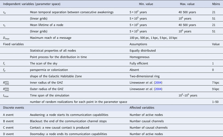
We implemented the simulation of a regular grid of models varying over the parameter space, which covers 5204 models. For each model, we simulated several realizations with different random seeds, adding up a total of 158546 simulation runs. The number of random realizations varies from one (for the densest populated models) up to 50 (for the sparsely populated models). The parameters for the temporal aspects of the simulation (the mean waiting time for the next awakening, τa, and the mean lifetime, τs) cover the ranges 102–106 years, with two linear partitions of 21 values (102–40 500 years) and 51 values (5 × 10⁵–106 years) for each parameter. This partition was chosen after the requirement of the software to take linear bins, aiming at a better sampling of the low τa and low τs region of the parameter space. For the D max parameter, we take the values 100 pc, 500 pc, 1 kpc, 5 kpc and 10 kpc. In Table 1 we show the three variable parameters, the ranges of their values and the number of bins that have been explored in the numerical experiments. We also show the set of fixed parameters that take part in the simulation, their values and the hypotheses that they represent.
Definition of independent variables and adopted values for fixed parameters that are part of the simulation

Variable parameters define the spatial and temporal structure of the process and the maximum reach of the messages.
As a product of the simulations, several quantities can be obtained. Some of them are directly derived from the discrete events, namely, the ID of emitting and receiving nodes and the position in the Galaxy. We also save the times of each of the events that are relevant to keep track of the number of nodes for each simulation, i.e., the times of the four types of events. The times of C-type and B-type events are used to derive the number of contacts. We also obtain quantities that represent the properties of the nodes, for example, the total time elapsed between the A-type and the D-type of each node, which represent their corresponding lifetimes. The time span of a node listening another or being listened by another node can also be derived by keepig track of the times of the events in a simulation. This way we can also compute the distribution in the simulated galaxy of nodes that reach contact, the distributions of the waiting times until the first contact or the distributions of waiting times until the next contact. The following properties of the population of nodes can also be derived: the fraction of the lifetime a node is listening to at least another node (i.e., within their light cone), the age of contacted nodes at first contact, the fraction of nodes where the first contact is given at the awakening, the distribution of the number of contacts for each node, the distribution of the number of contacts as a function of the age of the node, the number of contacts as a function of time in the Galaxy, the fractions of nodes that succeed in making contact and the distribution of distances between contacted nodes. Another useful derived quantity is the duration of two-way communication channels or the fraction of contacts that admit a response. It is also possible to analyse the relations between the distance to node versus the time of two-way communications, the distance to node versus the age of contacted node, the age of a node and the maximum number of contacted nodes before the D-type event, or the lifespan of a node versus the maximum number of contacts. All these quantities can be analysed as a function of the simulation parameters.
Membership to the network of connected nodes
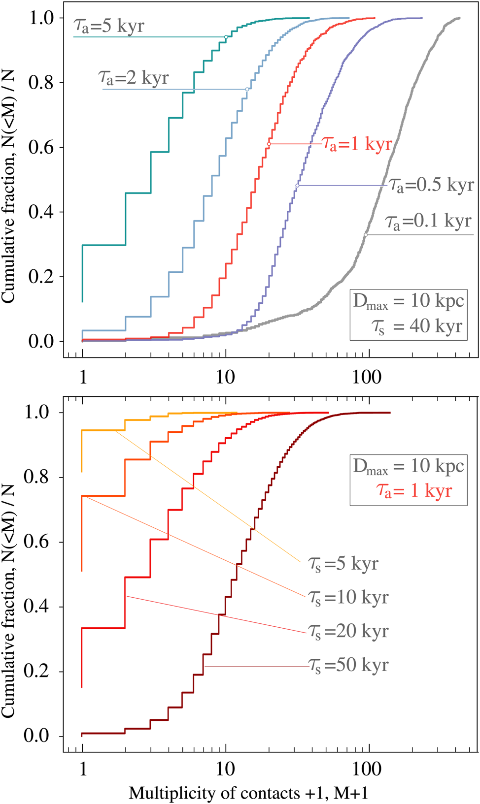
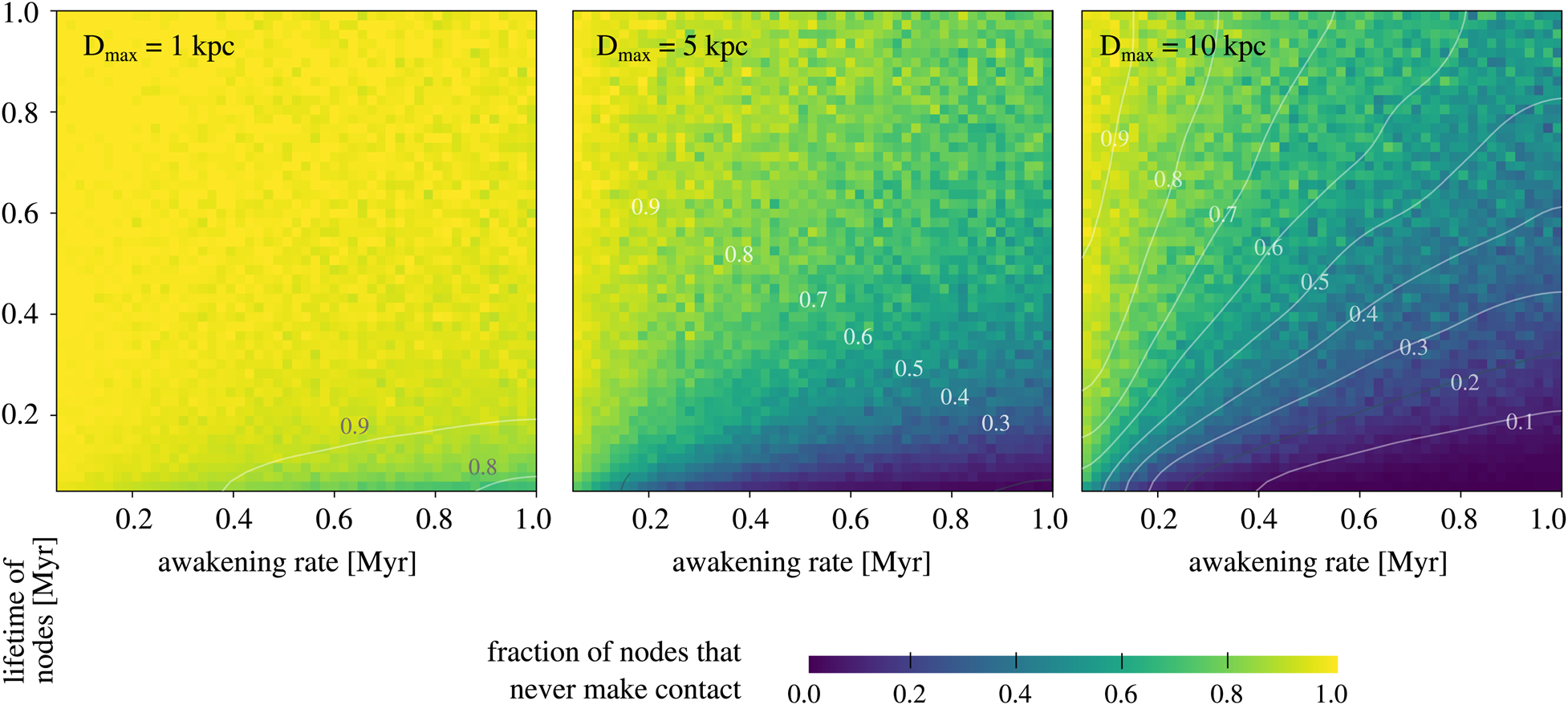
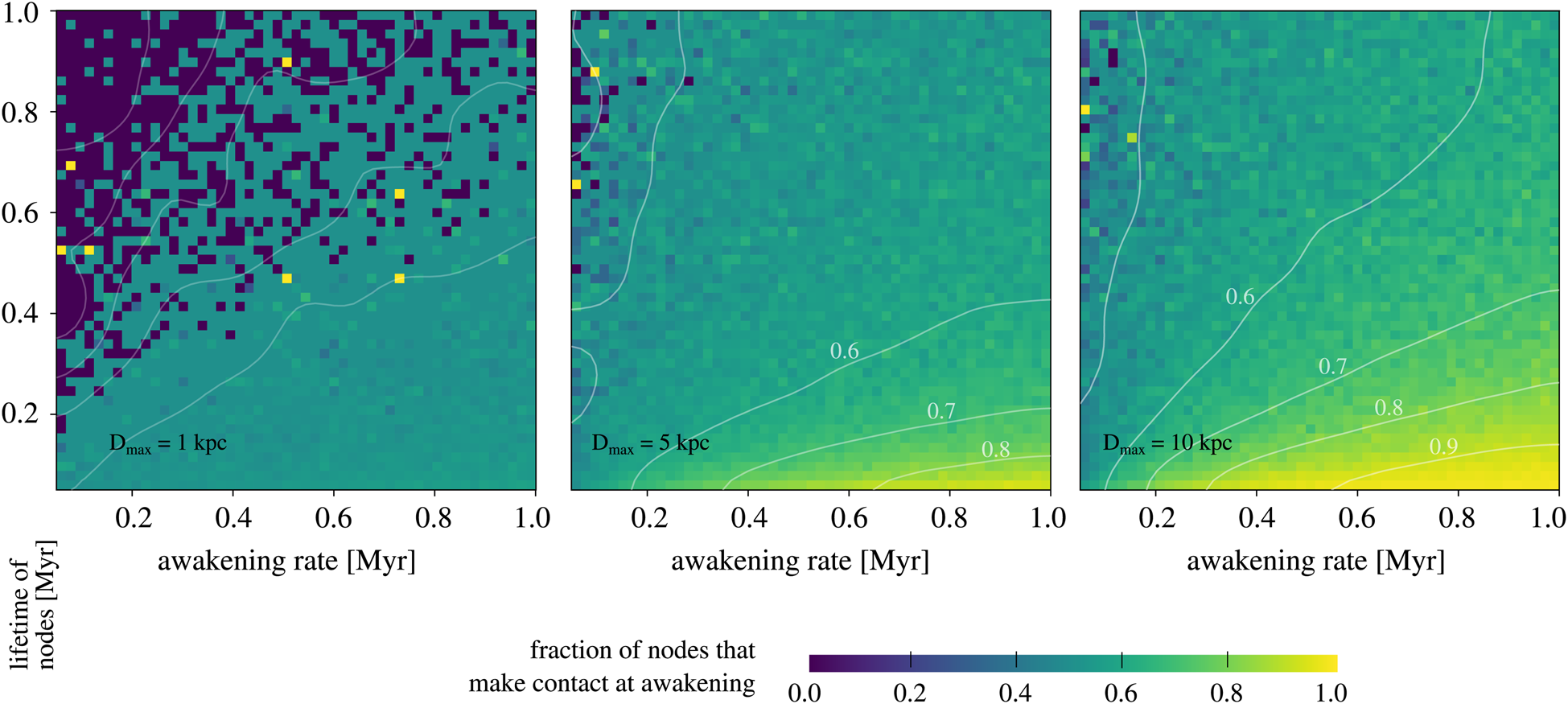
In Fig. 3 we show the empirical cumulative distributions of the number of contacts for nodes in six different samples, including short and long lifetimes, dense and sparse spatial distribution and D max = 10 kpc. As it can be seen, the mean lifetime is more determinant than the mean awakening rate (dense and sparse, represented by a different shade) for the number of contacts. The model with a dense awakening in the timeline (low τa) maximizes the number of contacts, reaching a maximum of more than 300 contacts for a single node. This case, however, requires that a new node appears in the Galaxy every 100 years on average. Similarly, the model with long lifetimes has the maximum number of contacts, reaching nearly 100 contacts for each node in its entire lifetime. This is considerably larger than any model with a shorter lifetime, which produce a number of contacts of at most the order of ten contacts per node. It is expected then that a model where nodes appear with a high frequency and have very long lifetimes can reach tens of contacts on the full time period between t A and t D. On the other side, a model where the activation of new nodes requires a large waiting time and the survival time is short, contacts are extremely rare. We should point out that this plot has a logarithmic scale on the x-axis, and it is the cumulative, not differential, empirical distribution. Therefore, the differences in the number of contacts for different models are large. This is a consequence of the wide range in both τa and τs covered in the simulations. With these ranges, the fraction of nodes with no contact ranges from nearly zero up to one. This analysis is made in order to explore the behaviour of the SC3Net model. In Fig. 4 we show 2D colour maps with the fraction of nodes in the simulations that never make contact (i.e., never listen to another node), as a function of the mean lifetime (τs, in the range 5 · 104–106 years) and the mean awakening time (τa, in the range 5 × 10⁴–106 years), for three different values of the maximum signal range, D max = 1 kpc (left panel), D max = 5 kpc (middle panel) and D max = 10 kpc (right panel). A clear pattern emerges, showing that the probability for a node of making causal contact with at least another node during their entire lifetime increases with increasing D max, increasing τs and decreasing τa, following a roughly linear dependence with the three parameters. The results of the simulations that comprise the full range of values for τa and τs from 5 × 10² to 106 years (not shown in the figures) maintain a similar trend. The number of nodes that do not succeed in reaching the causal contact regions of other nodes is a useful indicator of the degree of isolation. On the other hand, there is also the chance that a number of nodes are already in the causal contact region of other nodes, at the time of their A-type events. The fraction of nodes that make the first contact at the awakening event is shown in Fig. 5, as a function of the mean lifetime (τs, in the range 5 × 10⁴–106 years) and the mean awakening time (τa, in the range 5 × 10⁴–106 years). The three panels correspond to different values of the maximum signal range: D max = 1 kpc (left panel), D max = 5 kpc (middle panel) and D max = 10 kpc (right panel). The dependence of this metric with the three parameters is roughly linear in all cases.
Empirical cumulative distributions of the number contacts for nodes in different samples and with D max = 10 kpc. The upper panel shows the variation of the distribution as a function of the τa parameter, including the values 0.1, 0.5, 1, 2 and 5 kyr. All the curves correspond to models with τs = 40 kyr and D max = 10 kpc. The bottom panel corresponds to τa = 1 kyr and D max = 10 kpc, and the following values of τs: 5, 10, 20 and 50 kyr. Cumulative distributions can be used to visualize the probability of a random node of having more than M contacts in a given model. For example, in the upper panel the probability of a random node having more than ten contacts is nearly one for the model with the smallest τa value, and nearly zero for the model with the largest τa value.

The fraction of constrained causal contact nodes that never make contact (listening) as a function of τa and τs, for D max = 1 kpc (left panel), D max = 5 kpc (middle panel), and D max = 10 kpc (right panel). The values of τa and τs are in the range 5× 10⁵–106 years. The matrix is shown as obtained from the simulations, and the level curves are shown for the smoothed matrix.

The fraction of constrained causal contact nodes that make contact at the moment of the awakening (i.e., t A = t C), as a function of τa and τs, for D max = 1 kpc (left panel), D max = 5 kpc (middle panel) and D max = 10 kpc (right panel). The values of τa and τs are in the range 5 × 10⁵–106 years. The matrix is shown as obtained from the simulations, and the level curves are shown for the smoothed matrix.

Waiting time for a first contact
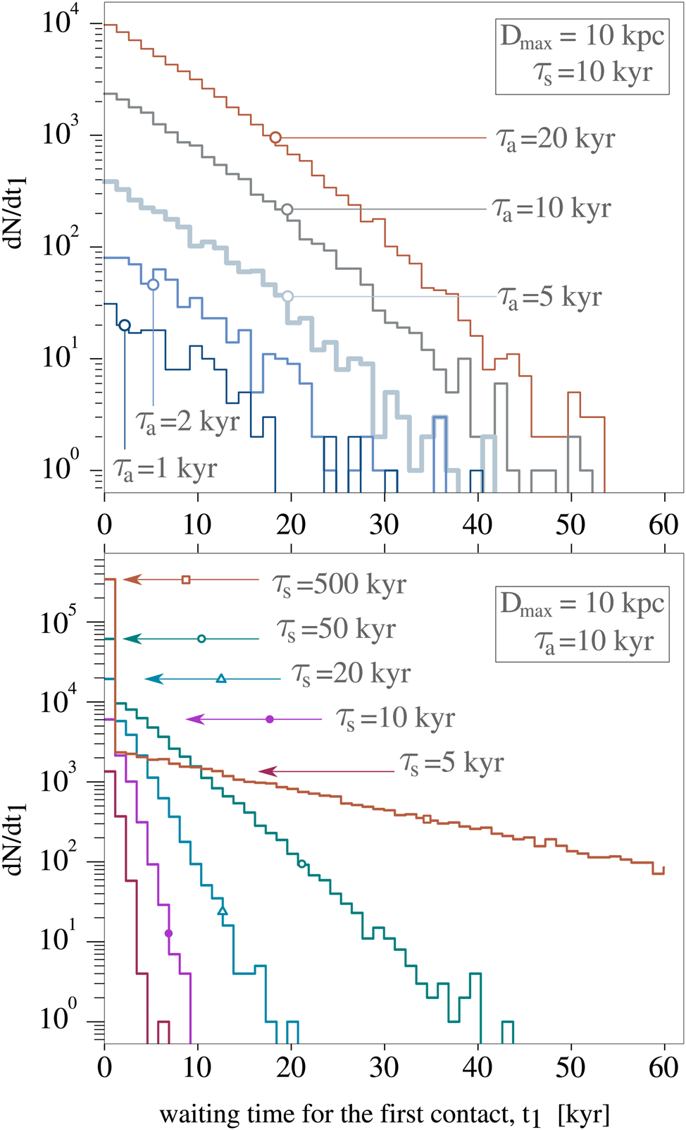
In this subsection we analyse the distribution of the waiting times for a first contact. Such distribution can be considered to compute the probability for a random node to carry out the searching of other nodes and spend a given time until the first contact is made, under the hypotheses of the experiment. In Fig. 6 we show the histograms of the mean waiting times for the first contact, for several models. Upper panel (a) shows the histograms for several values of the mean awakening time τa, with the mean survival time τs of 10 kyr. Lower panel (b) shows the histograms for several values of τs, with τa = 10 kyr. In both panels the value of D max is set to 10 kpc. As it can be seen, there is a clear trend where the number of nodes that require a time t 1 to make the first contact decreases exponentially with the time t 1. The fraction of the nodes that have made at least one contact, as a function of the elapsed time since the awakening, is computed with respect to the total number of nodes that make causal contact at least one time in the time range from the A-type up to the D-type events. From a frequentist approach, the cumulative fraction of contacts from the awakening (t = 0 years) up to a given time are related to the estimation of the probability of listening during that time interval and reaching to causal contact region of at least another node. The complement of this value is the probability of observing in a time interval with no success, i.e., without ever happening a C-type event. Clearly, this probability diminishes with time and tends to zero for large time periods, meaning the node will eventually enter into the light cone of other nodes. Remarkably, in densely populated models there is a clear excess at t 1 = 0 years. That is, for a short period of time the initial moment is the most promising for making a (causal) contact, for a given technology. This is given by the fact that at the awakening event, many nodes are already on the light cones of other nodes, so that the awakening time offers the best chance of making contacts. This offers a new approach to SETI programs, where the search for new communication technologies or the exploration of new communication channels has a fundamental role and could be more efficient than long observation programs.
Histograms of the mean waiting times for the first contact, for several models. Upper panel shows the histograms for several values of τa, and τs = 10 kyr and D max = 10 kpc. Bottom panel shows the histograms for several values of τs, with τa = 10 kyr and D max = 10 kpc. The arrows indicate the sample and highlight the values of the first waiting time bin, which has a clear excess for the models with larger τs values. The choice of these models was made in order to show the trends in the results as a function of the two temporal parameters.

Discussion
We have presented a stochastic model (SC3Net) to analyse the network of constrained causally connected nodes in a simplified Galaxy. It represents an idealized scenario of perfectly efficient emitters and receivers with the restriction of a maximum distance separation. These emitters and receivers correspond to nodes that form a communication network whose properties depend on their density and mean survival time. The statistical analysis of the model allows to estimate the probabilities for a random node and for a given model instance of making contacts with other nodes, along with the waiting times and durations of such contacts. Using numerical simulations, we implemented this model to explore the three-dimensional parameter space, considering a grid of mean time separations between the activation of new nodes in the range 500–106 years. Additionally, we explore a grid of the mean survival times between 500 and 106 years, and values for the maximum distance range of signals of 100 pc, 500 pc, 1 kpc, 5 kpc and 10 kpc. The simulation of each parameter point was performed several times with different random seeds in order to improve the confidence of the derived quantities.
Although the simulations use several hypotheses, we argue that the model is not worthy of further complexity, given the limited knowledge about the origin and persistence of life in the Galaxy. The implementation of more detailed or sophisticated models would increase the number of free parameters without any improvement in their predictive power. Thus, we take advantage of the simplicity of the model to explore the parameter space in order to gain insight on the consequences of different scenarios for the search of intelligent life. Our analysis is not centred in obtaining the odds for the Earth to make contact with another civilization. Instead, we focus on obtaining a statistical, parameter-dependent description of the possible properties of the communication networks that comprise sets of nodes with broadcasting and reception capabilities. This causally connected nodes are sparsely distributed in both space and time, making analytical treatments difficult and justifying the simulation approach.
Under the hypotheses of our experiments, we conclude that a causal contact is extremely unlikely unless the Galaxy is densely populated by intelligent civilizations with large average lifetimes. This result is qualitatively similar to the results presented by several authors, which state that a contact between the Earth and another intelligent civilization in the Galaxy is quite unlikely, provided the maximum distance of the signal and the lifetime of the emitter are not large enough. This analysis supports the idea that, in order to increase the possibilities of a contact, more active strategies of the emitter would be required. Some proposals in this direction include interstellar exploration, colonization and settlement (Brin Reference Brin1983; Došović et al. Reference Došović, Vukotić and Ćirković2019; Galera et al. Reference Galera, Galanti and Kinouchi2019), although it would require large temporal scales. Došović et al. (Reference Došović, Vukotić and Ćirković2019) use probabilistic cellular automaton simulations to explore the parameter space of a model with colonization and catastrophic events. According to the timescales involved, their results could explain the Fermi paradox. Although our work does not take into account the colonization hypothesis, it does consider catastrophic events implicitly in the mean value and distribution of the lifetime, τs. Other strategies could also increase the probability of contacts, for example, panspermia (e.g., Starling and Forgan Reference Starling and Forgan2014) or self-replicating probes (e.g., Barlow Reference Barlow2013), although they would be too slow to make a significant impact on the communication network among intelligent civilizations. Our results are also consistent with those presented by Grimaldi (Reference Grimaldi2017), who estimates an upper limit for the mean number of extraterrestrial civilizations that could contact Earth using Monte Carlo simulations, from a statistical model where the width of the Galactic disk is not negligible. Unlike most of the studies that make use of statistical models or simulations (Ćirković Reference Ćirković2004; Smith Reference Smith2009; Bloetscher Reference Bloetscher2019), our approach does not relay on the Drake equation. Thus, it does not need a detailed description or modelling of the physical processes that give rise to intelligent life. However, we argue that it is a valid empirical formulation to discuss the probabilities of contact and the time scales involved in the problem. Ours is an alternative to the method proposed by Balbi (Reference Balbi2018a), who performs an analysis based on the Earth with a different model. Despite those differences, their results and ours are in general agreement.
We have also found that there is a balance between the density of nodes and the mean lifetime since, as expected, a lower density can be compensated by a longer active time period. However, a large number of nodes does not easily compensate their short lives to reach the same probability of causal contact than in the case of a less populated galaxy but with very ancient civilizations. In all cases, for a short period of time (for instance, the time SETI programs have been active on Earth), the maximum probability of making a contact occurs at the moment of the awakening. This suggests the possibility that an alternative SETI strategy could be the search for alternative message carriers, for the case in which the search has not been performed on the adequate channels. Then, if a contact is produced for the first time, the origin of the signal is more likely to be very old. Also, the chances of entering the causal connected zone of a node do not grow linearly, but favour the first period of 105 years.
In the approach of this work, we have used computer simulations to address the problem of the probabilities of causal contacts between locations in the Galaxy with the possibility of sending and receiving messages. Instead of making a number of assumptions, we have explored the parameter space, reducing the problem to only three parameters and a few simple hypotheses to perform a complete model for the population and communication network in the Galaxy. This allows to consider the Fermi paradox from a new perspective, and to propose an alternative treatment for the number of intelligent emitter/receivers. If the time intervals between the rise and fall of civilizations are short compared to the time required for an electromagnetic signal to travel the large distances in the Galaxy, then the number of contacts would be limited to a low number.
The short time interval between the rise and fall of civilizations, compared to the age and extension of our Galaxy, is a fundamental limitation for the number of contacts. The temporal dimension, which is missing in the Drake equation, is a key factor to understand the network of contacts on different scenarios.
Acknowledgement
This work was partially supported by the Consejo Nacional de Investigaciones Científicas y Técnicas (CONICET, Argentina), the Secretaría de Ciencia y Tecnología, Universidad Nacional de Córdoba, Argentina, and the Universidad Católica de Córdoba, Argentina. This research has made use of NASA's Astrophysics Data System. Plots and simulations were made with software developed by the authors the python language. Plots were postprocessed with inkscape. Simulations were run on the Clemente cluster at the Instituto de Astronomía Teórica y Experimental (IATE).
Conflict of interest
No competing financial interests exist.