1 Introduction
The liquid metal fusion blanket, such as the helium cooled lead lithium blanket (Mistrangelo & Bühler Reference Mistrangelo and Bühler2009), has been intensively investigated for application in fusion reactors. It serves as a coolant and breeder material. Generally, the heat transfer inside the blanket is more efficient if the flow is turbulent or vortical. An experimental investigation in Brouillette & Lykoudis (Reference Brouillette and Lykoudis1967) revealed that a phenomenon of the transition to a laminar state in magnetohydrodynamics (MHD) channel flow will reduce the heat transfer coefficient. A technique noted in Sukoriansky et al. (Reference Sukoriansky, Klaiman, Branover and Greenspan1989) is used to enhance heat transfer by placing obstacles inside the blanket to promote turbulence or generate vortical structures. Another engineering problem in electromagnetic metallurgy is the production of clean metal, free from oxides and other types of non-metallic inclusions. Electromagnetic filtration (El-Kaddah, Patel & Natarajan Reference El-Kaddah, Patel and Natarajan1995) is a technology that purifies the molten metals and removes these unneeded non-metallic inclusions. It is important to know the wake structures behind such inclusions while they are transported in MHD flow since their traces are determined by the wake structures (Ern et al. Reference Ern, Risso, Fabre and Magnaudet2012). Therefore, understanding the influence of a magnetic field on the wake structure around an obstacle can provide valuable knowledge for practical application.
The problem considered in the present paper is the wake structure and transition process behind a stationary sphere with the influence of a suddenly imposed streamwise magnetic field. The flow of a viscous fluid past a stationary sphere may be naturally considered a canonical case of a general family of immersed obstacle flow with widespread applications. Investigations of wake structure and instability past a fixed sphere without a magnetic field has been studied by a number of researchers. A global stability analysis of Natarajan & Acrivos (Reference Natarajan and Acrivos1993), some direct numerical simulation (DNS) of Johnson & Patel (Reference Johnson and Patel1999), Ghidersa & Dušek (Reference Ghidersa and Dušek2000) and Tomboulides & Orszag (Reference Tomboulides and Orszag2000) and the detailed experiments by Ormières & Provansal (Reference Ormières and Provansal1999) all found a consistent scenario of transition. The first transition of this flow occurs at
 $Re\approx 210$
. Compared with the flow past a circular cylinder where the first transition at
 $Re\approx 47$
is a Hopf bifurcation from a two-dimensional steady to a two-dimensional unsteady periodic flow (Williamson Reference Williamson1996), the first bifurcation encountered in the sphere wake is a transition from the steady, axisymmetric wake to the steady, non-axisymmetric, double-thread wake. This bifurcation leads to a stationary and planar reflectional symmetry state. The normal orientation of this plane, in principle, is random but is presumably determined by perturbations in experiments or numerical biases resulting from sweep directions in the solver (Johnson & Patel Reference Johnson and Patel1999). The double-threaded wake consists of two steady streamwise vortices which are opposite in sign and the recirculation region behind sphere is tilted. A secondary Hopf bifurcation subsequently occurs at
 $Re\approx 270$
. The double-thread wake itself is observed to become unstable in a periodic state within a symmetric plane determined by the first bifurcation. This is called reflectional symmetry preserving by Fabre, Auguste & Magnaudet (Reference Fabre, Auguste and Magnaudet2008). Close to the threshold, it manifests itself in small-amplitude oscillations without a distinct vortex shedding. The double-thread wake shows wave-like oscillations, as reported in the experimental work of Magarvey & MacLatchy (Reference Magarvey and MacLatchy1965) when
 $270\leqslant Re\leqslant 290$
and Sakamoto & Haniu (Reference Sakamoto and Haniu1990) when
 $Re<300$
. The oscillations then grow in magnitude with an increasing Reynolds number and eventually vortex loops begin shedding from the sphere (so-called hairpin vortices) at
 $Re=300$
. Dye lines in experiments by Johnson & Patel (Reference Johnson and Patel1999) revealed the shedding of large-amplitude hairpin vortices. Vortical structures in the simulation by Tomboulides & Orszag (Reference Tomboulides and Orszag2000) showed that the wake contained streamwise vorticities of alternating sign and different magnitudes. As the Reynolds number is further increased, simulations by Mittal (Reference Mittal1999) showed that the wake became irregular, fully three-dimensional and no longer retained a plane symmetry while
 $Re>355$
. Experiments by Sakamoto & Haniu (Reference Sakamoto and Haniu1990) measured the frequency presented in the unsteady wake, which showed that the flow transitioned from a single frequency to an almost chaotic system when
 $Re>420$
.
With the existence of an external magnetic field, MHD flow characteristics are dominated by two dimensionless parameters. One is the Reynolds number, which gives a measure of the ratio of inertial to viscous forces. The other is the interaction parameter, which represents the ratio of electromagnetic to inertial forces. Any movement of a conducting fluid, which is non-parallel to the magnetic field, will generate electric currents. Consequently, the interaction of these currents with the external magnetic field gives rise to an MHD force, known as the Lorentz force (Davidson Reference Davidson2001), that greatly changes the flow patterns. For MHD flows without an obstacle, the evolution of turbulent flow under the influence of a magnetic field has been researched theoretically (Sommeria & Moreau Reference Sommeria and Moreau1982; Davidson Reference Davidson2001) and the effect of the magnetic field can be described as the propagation of momentum and vorticity along the magnetic field direction since vortices aligned with a magnetic field are damped more weakly than those perpendicular to the magnetic field lines. Some experiments about the influence of magnetic fields on turbulence can be found in Alemany et al. (Reference Alemany, Moreau, Sulem and Frisch1979), Klein & Pothérat (Reference Klein and Pothérat2010), Verhille et al. (Reference Verhille, Khalilov, Plihon, Frick and Pinton2012). Introducing a cylinder as an obstacle in the flow to promote turbulence or generate vortical structures has been fully investigated. In the experiment of Kolesnikov & Tsinober (Reference Kolesnikov and Tsinober1974), the cylinder axis was aligned with the magnetic field and for a strong magnetic field the axes of the vortices behind the cylinder were aligned with the magnetic field. Similar results were reported by the simulation in Kanaris et al. (Reference Kanaris, Albets, Grigoriadis and Kassinos2013). Under the condition of a streamwise magnetic field, both the experiments (Lahjomri, Caperan & Alemany Reference Lahjomri, Caperan and Alemany1993) and numerical simulations (Mutschke et al. Reference Mutschke, Gerbeth, Shatrov and Tomboulides2001) found that the eddies were narrowed, and by increasing the interaction parameter, the detachment from the cylinder was suppressed and the flow was transitioned to a two-dimensional state at the end. The magnetic field along the transverse direction has also been investigated (Kalis et al. Reference Kalis, Tsinober, Shtern and Shcherbinin1965; Mutschke et al. Reference Mutschke, Gerbeth, Shatrov and Tomboulides2001). The orientation of the magnetic field has a dramatic influence on vortical structure. In summary, the magnetic field stabilizes the flow, delays flow separation and shifts the transition to unsteadiness into higher critical thresholds. Some other obstacles to generating vortices are suggested such as a square cylinder (Mück et al. Reference Mück, Günther, Müller and Bühler2000) and grid bars (Branover, Eidelman & Nagorny Reference Branover, Eidelman and Nagorny1995).
However, studies relevant to MHD flows past a sphere are rather scarce. Chester (Reference Chester1957) studied the effect of a magnetic field on Stokes flow past a sphere. An Oseen approximation method was extended to an MHD flow past a sphere in Goldsworthy (Reference Goldsworthy1961). A two-dimensional axisymmetric model was used in Sekhar, Sivakumar & Kumar (Reference Sekhar, Sivakumar and Kumar2005), which only focused on steady and axisymmetric situations. Yonas (Reference Yonas1967) made direct drag measurements on a sphere in conducting liquid sodium with an aligned field and found that the drag coefficient was proportional to the square root of the interaction parameter for a large magnetic field. Their experiments indicated that a relatively weak magnetic field was able to completely dampen the dominant frequencies which had existed in a hydrodynamic situation. Similar results were reported by Maxworthy (Reference Maxworthy1962), who noted a non-oscillatory wake structure for a certain interaction parameter. It is noted that the liquid metal used in the experiment is opaque, so any visualization technology based on an optical method, such as dye visualization, is useless for visualizing the wake structure behind the sphere. Therefore, three-dimensional simulation is needed to give a thorough understanding of the influence of a sudden streamwise magnetic field on the fluid dynamics and the wake structure of a flow past a sphere.
As reviewed above, the wake structure behind a sphere without a magnetic field will undergo a series of well-defined transitions with Reynolds number up to
 $300$
, such as from a steady axisymmetric flow to a steady plane symmetric flow and then to an unsteady periodic flow. Particularly interesting throughout the literature is how a streamwise magnetic field affects the fluid dynamics and wake structures behind a sphere. The present work attempts to answer this question by numerically solving the flow in a three-dimensional, time-dependent fashion. The flow is first simulated for a long time until a ‘stable’ state is obtained. Then a uniform streamwise magnetic field is imposed to investigate how the Lorentz force modifies the wake structure behind a sphere with Reynolds number up to
 $300$
, which covers the first and second Hopf bifurcations in its hydrodynamics counterpart.
This paper is organized as follows. Section 2 describes the mathematical model and numerical method. The numerical results for the steady axisymmetric flow affected by a magnetic field are presented in § 3. Later, the influence of magnetic field on a steady plane symmetric flow is shown in § 4. Following this, the results for an unsteady flow affected by a magnetic field are given. In § 6, the drag and lift coefficient are discussed. Finally, a summary is given.
2 Mathematical model and numerical method
An electric conducting incompressible Newtonian fluid with density
 $\unicode[STIX]{x1D70C}$
, kinematic viscosity
 $\unicode[STIX]{x1D708}$
and electrical conductivity
 $\unicode[STIX]{x1D70E}$
, is considered under the influence of a suddenly imposed streamwise magnetic field
 $\boldsymbol{B}$
. For most cases of liquid metal flow in industrial applications, the magnetic Reynolds number is very small, and thus the induced magnetic field is found to be negligible when compared with the imposed magnetic field. Hence, a so-called quasi-static approximation (Davidson Reference Davidson2001; Moreau Reference Moreau2013) of the MHD equations is invoked when the magnetic Reynolds number is assumed to be much smaller than unity
 $Rm=\unicode[STIX]{x1D707}\unicode[STIX]{x1D70E}UL\ll 1$
, where
 $\unicode[STIX]{x1D707}$
is the fluid magnetic permeability. Under this assumption, the non-dimensional magnetohydrodynamic equations governing the flow can be written as
 $$\begin{eqnarray}\displaystyle & \displaystyle \frac{\unicode[STIX]{x2202}\boldsymbol{u}}{\unicode[STIX]{x2202}t}+(\boldsymbol{u}\boldsymbol{\cdot }\unicode[STIX]{x1D735})\boldsymbol{u}=-\unicode[STIX]{x1D735}p+\frac{1}{Re}\unicode[STIX]{x1D6FB}^{2}\boldsymbol{u}+N(\boldsymbol{J}\times \boldsymbol{B}), & \displaystyle\end{eqnarray}$$
 $$\begin{eqnarray}\displaystyle & \displaystyle \unicode[STIX]{x1D735}\boldsymbol{\cdot }\boldsymbol{u}=0, & \displaystyle\end{eqnarray}$$
 $$\begin{eqnarray}\displaystyle & \displaystyle \boldsymbol{J}=-\unicode[STIX]{x1D735}\unicode[STIX]{x1D719}+\boldsymbol{u}\times \boldsymbol{B}, & \displaystyle\end{eqnarray}$$
 $$\begin{eqnarray}\displaystyle & \displaystyle \unicode[STIX]{x1D735}\boldsymbol{\cdot }\boldsymbol{J}=0. & \displaystyle\end{eqnarray}$$
The dimensionless flow variables appearing in (2.1)–(2.4) are obtained from their dimensional counterparts. The variables
 $t$
,
 $\boldsymbol{u}$
,
 $p$
,
 $\boldsymbol{J}$
,
 $\boldsymbol{B}$
,
 $\unicode[STIX]{x1D719}$
denote the dimensionless time, velocity, pressure, current density, imposed magnetic field and electric potential. They are scaled with
 $L/U,U,\unicode[STIX]{x1D70C}U^{2},\unicode[STIX]{x1D70E}UB,B$
and
 $LUB$
, respectively. Here the uniform inflow velocity
 $U$
is the characteristic velocity scale and
 $L$
is the characteristic length scale. Two dimensionless parameters that appeared in the momentum equation (2.1) are the Reynolds number
 $Re=UL/\unicode[STIX]{x1D708}$
and the interaction parameter
 $N=\unicode[STIX]{x1D70E}LB^{2}/\unicode[STIX]{x1D70C}U$
. For a variety of applications, the essential balance of forces in the Hartmann layer is established between the electromagnetic force and the viscous force (Hunt Reference Hunt1965). The ratio of these forces can be expressed in terms of the Reynolds number and the interaction parameter as
 $NRe=Ha^{2}$
, where
 $Ha=LB\sqrt{\unicode[STIX]{x1D70E}/\unicode[STIX]{x1D70C}\unicode[STIX]{x1D708}}$
is the Hartmann number. A Poisson equation for the electric potential can be derived from the solenoidal current field of (2.4) and Ohm’s law of (2.3) as
 $$\begin{eqnarray}\unicode[STIX]{x1D735}\boldsymbol{\cdot }\unicode[STIX]{x1D735}\unicode[STIX]{x1D719}=\unicode[STIX]{x1D735}\boldsymbol{\cdot }(\boldsymbol{u}\times \boldsymbol{B}).\end{eqnarray}$$
This Poisson equation will be solved to get the electrical potential, which will be employed to calculate the current density based on Ohm’s law of (2.3) and the Lorentz force.
In an MHD flow, guaranteeing charge conservation in a non-uniform grid arrangement is a true challenge (Smolentsev et al. Reference Smolentsev, Badia, Bhattacharyay, Bühler, Chen, Huang, Jin, Krasnov, Lee and de les Valls2015). Ni et al. (Reference Ni, Munipalli, Huang, Morley and Abdou2007) proposed a consistent and conservative scheme to effectively solve this problem on an arbitrary collocated grid system, in which all the variables are located in the cell centre while the current density fluxes are located on cell faces. A second-order accurate centred-difference scheme with skewness corrections is used for the discretization of the convective and diffusive terms. Then the fractional-step method is used to solve the pressure–velocity coupled equation. The time integration of the flow equations is done using the Adams–Bashforth scheme to explicitly update the convective term and the Crank–Nicolson scheme for the diffusive term. Detailed validation and verification can be found in Ni et al. (Reference Ni, Munipalli, Huang, Morley and Abdou2007).
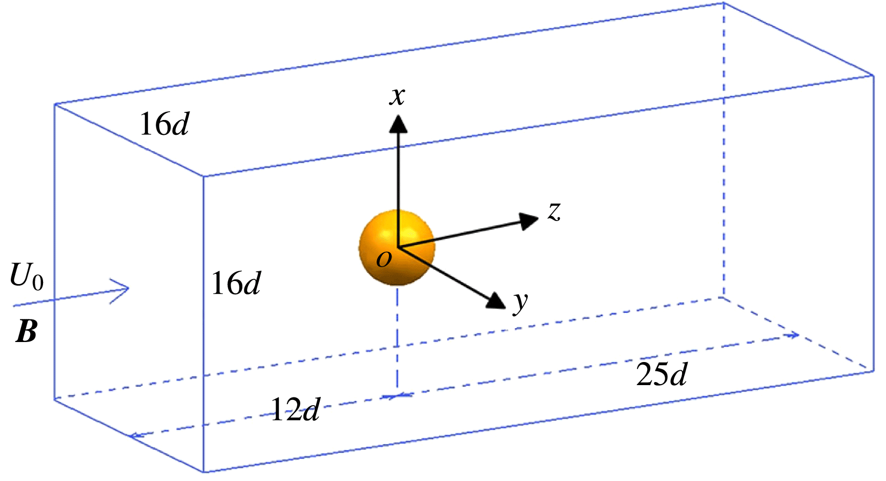
Schematic of diagram for the flow configuration and related geometrical parameters.

The geometry considered in the present study is shown in figure 1. It consists of a sphere of diameter
 $d$
at the axis of a rectangular duct which has the size of
 $16d\times 16d\times 37d$
. The duct inlet is placed at a distance of
 $12d$
upstream of the sphere, while the outlet is located at
 $25d$
behind the body. The choice of geometrical parameters ensures minimal distortion of the flow structures, due to the outer boundary conditions, while maintaining a reasonable computational cost. Since the present research mainly concerns the influence of a streamwise magnetic field on the wake structures behind the sphere, any wake–wall interpolations are excluded. Thus slip boundary conditions are set on the duct walls. At the inlet, a uniform velocity is given while a convective boundary condition is applied at the outlet. A no-slip boundary condition is imposed on the sphere. For MHD flow, there is an electric potential governing equation. The charge conservation law demands no electric currents enter or leave the domain. Hence, the condition
 $\unicode[STIX]{x2202}\unicode[STIX]{x1D719}/\unicode[STIX]{x2202}n=0$
is imposed on the sphere and the other boundary conditions are set as (Mück et al.
Reference Mück, Günther, Müller and Bühler2000)
 $$\begin{eqnarray}\frac{\unicode[STIX]{x2202}\unicode[STIX]{x1D719}}{\unicode[STIX]{x2202}n}=(\boldsymbol{u}\times \boldsymbol{B})\boldsymbol{\cdot }\boldsymbol{n}.\end{eqnarray}$$
The above equation is derived from the electric potential equation (2.5) and reduces to the requirement of zero normal component of the current at the boundary.
It is known that flow configuration is sensitive to various numerical and physical parameters such as the grid resolution, the domain size, the blockage and the boundary conditions. No wake–wall interaction is considered at the present research. We are concerned only with the grid resolution near the sphere and in the wake region. Based on parameters in this study, the grid resolutions of extreme parameters at
 $Re_{max}=300$
with
 $N_{min}=0$
and
 $N_{max}=10$
are tested, respectively. The computational domain is divided into a number of hexahedral cells. The estimation of boundary layer thickness at
 $Re=300$
in Tomboulides & Orszag (Reference Tomboulides and Orszag2000) is adopted here,
 $\unicode[STIX]{x1D6FF}=0.065d$
. Here, the distance between the nearest grid point and sphere surface is set with
 $\unicode[STIX]{x1D6FF}_{min}=0.01d$
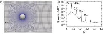
. There are 4–5 grid nodes to resolve the boundary layers. In order to have a good orthogonality, the grid is clustered in a concentric sphere and the spacing is increased with a ratio 1.1 away from sphere surface. Then ‘O’ grids and multi-blocks are set in other parts of the domain as seen in figure 2(a). Two different grid resolutions are tested at
 $Re=300$
with
 $N=0$
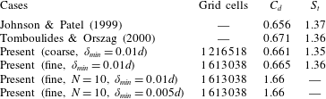
. The drag coefficient and Strouhal number agree well with previous results as shown in table 1. Figure 2(b) plots the power spectrum of the streamwise velocity component for a point downstream in the wake. The shedding frequency and its superharmonics are consistent with figure 15(b) in Tomboulides & Orszag (Reference Tomboulides and Orszag2000). Based on these results, the fine grid is chosen and it is sufficient to resolve wake flow behind the sphere.
Grid resolution test at
 $Re=300$
. (a) Grid expanded view in the vicinity of the sphere. (b) The power spectrum of the streamwise velocity component for the fine grid at
 $x=0,y=0,z=6d$
(log plot).

Grid independence test at
 $Re=300$
.

Furthermore, in an MHD channel flow (Moreau Reference Moreau2013), the thickness of the Hartmann layers, which are perpendicular to a magnetic field, is scaled with
 $\unicode[STIX]{x1D6FF}_{\bot }=O(Ha^{-1})$
. The thickness of Shercliff layers, which are parallel to a magnetic field, is scaled with
 $\unicode[STIX]{x1D6FF}_{\Vert }=O(Ha^{-1/2})$
. The Shercliff boundary layer is much thicker than the Hartmann boundary layer. However, these scaled thickness are both related to a flat wall. As for the sphere case, they may not be suitable. Kanaris et al. (Reference Kanaris, Albets, Grigoriadis and Kassinos2013) did a series of grid resolution tests for MHD flow around a cylinder and their research gives us a lot of reference and inspiration. Their Reynolds number and Hartmann number were up to 5000 and 280 (based on diameter), respectively, and the smallest grid element size normal to the cylinder surface was
 $0.005d$
. Their grid arrangement gave accurate results. The largest interaction parameter in the present research is
 $10$
and the corresponding largest Hartmann number is
 $Ha=(NRe)^{-(1/2)}=54.8$
. Suggested by grid resolution tests in Kanaris et al. (Reference Kanaris, Albets, Grigoriadis and Kassinos2013), it is reasonable that the height of the first layer of grid on the sphere surface is set as
 $0.01d$
in the present grid under the consideration of a Reynolds number and Hartmann number of no more than 300 and 54.8, respectively. It is noted that the vortical structure behind the sphere will be suppressed with a strong magnetic field. The grid resolution near the sphere surface is concerned when the magnetic field is strong. Two grids with different first grid resolution at
 $Re=300$
and
 $N=10$
are tested in table 1. The same drag coefficients confirm that the fine grid with
 $\unicode[STIX]{x1D6FF}_{min}=0.01d$
is also sufficient to resolve the present MHD flow.
3 Steady axisymmetric flow affected by magnetic field
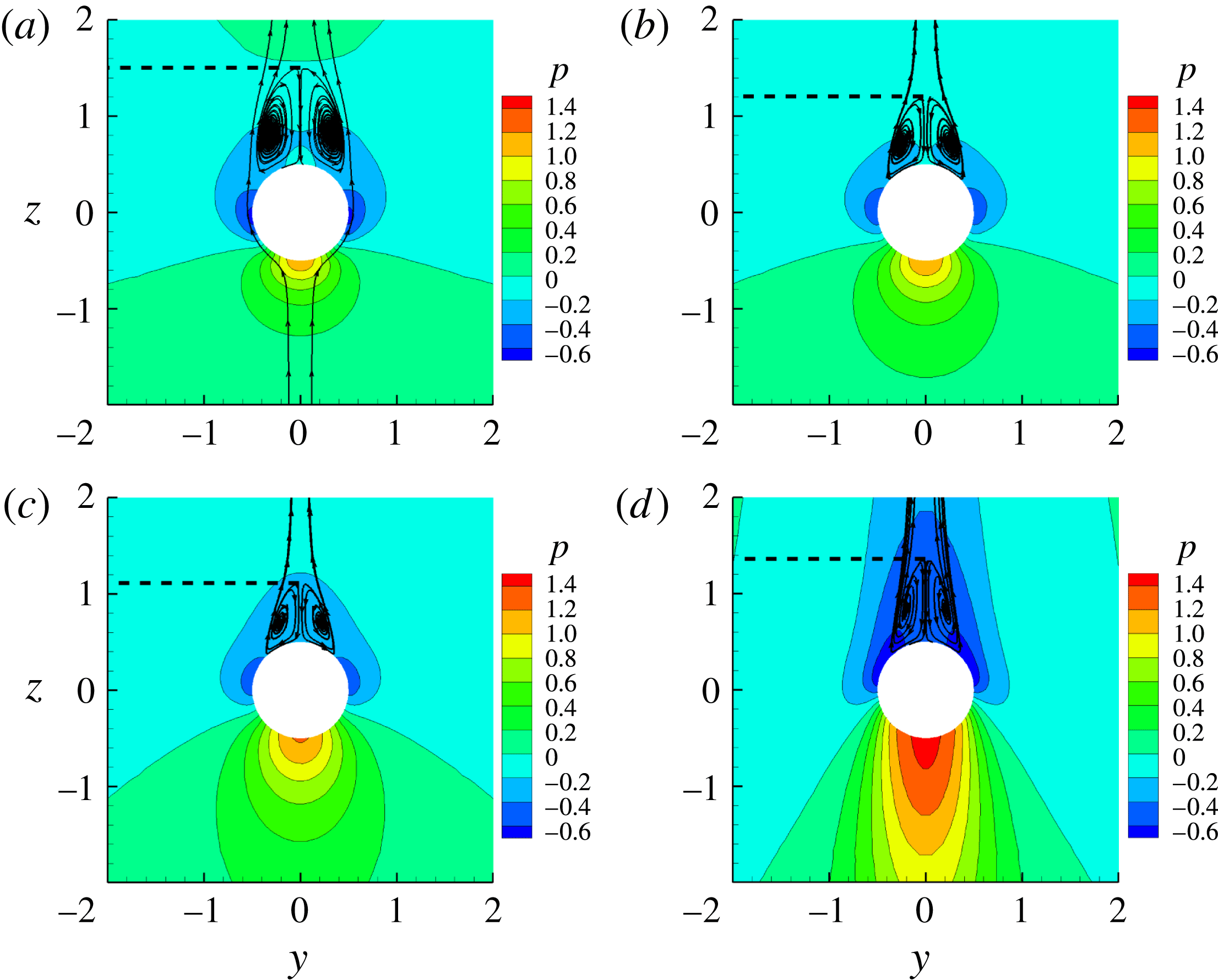
When the Reynolds number is between 20 and approximately 210, the flow is separated, steady, axisymmetric and topologically similar with changes only in the separation location and the separation bubble length. Details can be found in Johnson & Patel (Reference Johnson and Patel1999). The pressure contours and streamlines at
 $Re=150$
with different interaction parameters are presented in figure 3. It is clearly seen that the flow topological structure remains the same after imposing a streamwise magnetic field. Since the magnetic field aligns with the axis of the separation bubble, the Lorentz force axisymmetrically acts on the separation bubble. It is known that the Lorentz force will suppress any flows that are not parallel to the magnetic field, and therefore longer stagnant regions ahead of and behind the sphere occur for a large interaction parameter. These regions correspond to high and low pressure zones as shown in figure 3.
Pressure contours and streamlines in the symmetric plane at
 $Re=150$
with different interaction parameters. (a)
 $N=0$
; (b)
 $N=1$
; (c)
 $N=2.4$
; (d)
 $N=10$
.

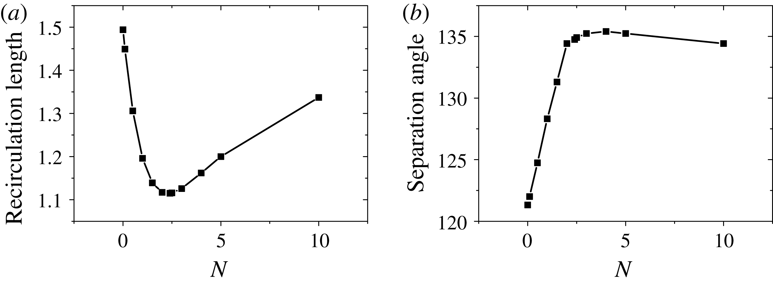
Shatrov, Mutschke & Gerbeth (Reference Shatrov, Mutschke and Gerbeth1997) found that a transverse magnetic field could lead to a complete suppression of recirculation on a two-dimensional flow past a cylinder. However, in figure 3, the length of the recirculation bubble at the rear stagnation point reduces from
 $N=0$
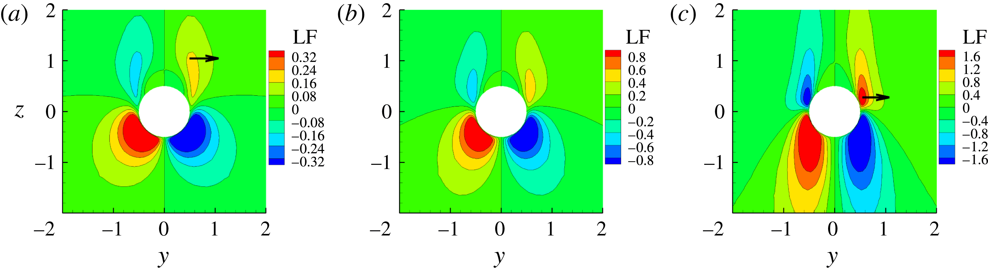
to 2.4. And with a larger magnetic field, the separation length is not suppressed but rather increasing. Figure 4 shows the axisymmetric Lorentz force contours in the same plane as figure 3. The direction of the Lorentz force is from left to right. Since it is axisymmetric, only the upper right part is analysed. It can be seen from the arrows that the Lorentz force mainly acts on the separation bubble tail at a small interaction parameter
 $N=0.1$
while the Lorentz force mainly acts on the head at a large interaction parameter
 $N=10$
. For a small interaction parameter case, the flow velocity has a large component perpendicular to the magnetic field at the tail of the recirculation bubble. Hence, it generates a Lorentz force, which will pull away outer streamlines at the tail of the recirculation bubble and make them flow downstream. The recirculation bubble becomes smaller, corresponding to a smaller recirculation length and a larger separation angle. With an increasing magnetic field, the size of the recirculation bubble becomes smaller. At the same time, convective flow from the upstream fluid to the rear of the sphere has a larger flow velocity component perpendicular to the magnetic field. The Lorentz force now mainly prevents this flow at a large interaction parameter case. Consequently, an inverse pressure gradient on the sphere surface near the arrow in figure 4(c) induces recirculation streamlines which add onto the outer surface of the original recirculation bubble. Now the recirculation length increases while the separation angle decreases.
Lorentz force contours in the symmetric plane at
 $Re=150$
with different interaction parameters. The direction is from left to right. The arrows indicate the main acting position of the Lorentz force. (a)
 $N=1$
; (b)
 $N=2.4$
; (c)
 $N=10$
.

The non-monotonic behaviour in the recirculation length and separation angle is caused by different acting positions of the Lorentz force. Figure 5 gives an overall picture of the behaviour of the recirculation length and separation angle versus the interaction parameter at
 $Re=150$
. The inflection points are approximately
 $N=2.4$
and
 $N=4$
, respectively. The reason for the different value of the inflection point is that it is more difficult to prevent convective flow into the rear of the sphere at the head of the recirculation bubble than to pull away outer streamlines at the tail of the recirculation bubble. The same non-monotonic behaviour was also found by Sekhar et al. (Reference Sekhar, Sivakumar and Kumar2005) for the case of two-dimensional axisymmetric flow around a sphere at
 $Re=100$
and
 $Re=200$
and Mutschke et al. (Reference Mutschke, Gerbeth, Shatrov and Tomboulides2001) for the case of flow around a circular cylinder at
 $Re=200$
.
Recirculation length and separation angle versus the interaction parameter at
 $Re=150$
. (a) Recirculation length. (b) Separation angle.

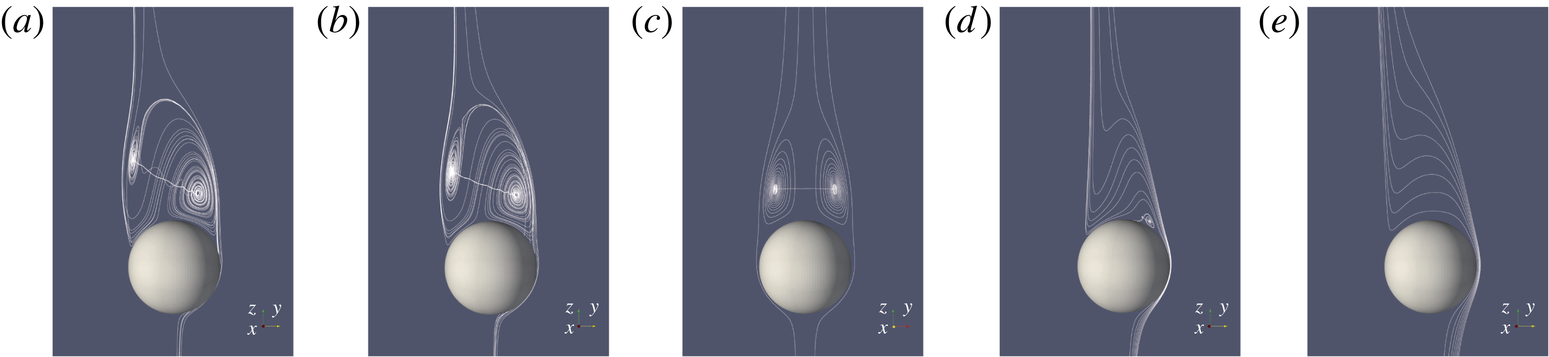
Three-dimensional streamlines projected on the symmetric plane at
 $Re=250$
with different interaction parameters. (a)
 $N=0$
; (b)
 $N=0.1$
; (c)
 $N=0.3$
; (d)
 $N=7$
; (e)
 $N=10$
.

4 Steady plane symmetric flow affected by magnetic field
The separation bubble is axisymmetric at a low Reynolds number and it grows in length until the Reynolds number reaches approximately 210. The first transition involves a (regular) symmetry-breaking topological change from a steady axisymmetric wake with an attached separation bubble to a steady plane symmetric wake consisting of two trailing counter-rotating vortices. This normal bifurcation at approximately
 $Re=210$
is associated with an azimuthal instability of the low-pressure core of the main axisymmetric bubble (Johnson & Patel Reference Johnson and Patel1999). The steady plane symmetric wake has a range of approximately
 $210<Re<270$
, which has been investigated experimentally by Magarvey & Bishop (Reference Magarvey and Bishop1961) and numerically by Johnson & Patel (Reference Johnson and Patel1999). These authors found that the wake within this regime was essentially self-similar or topologically identical. One case at
 $Re=250$
, which is within this regime, is considered here. It is apparent that the toroidal vortex has tilted in figure 6(a) and is no longer a closed separation bubble. Upstream fluid feeds the left spiral and serves as a source, where the fluid flows out and enters into the centre of right part of the vortex. Then the right spiral releases fluid into the wake after sending it up and around the left spiral. It is noted that the sizes of the left and right of the vortex ring are not constant in the azimuthal direction. The core of the toroidal vortex ring consists of an azimuthal vortex axis on both sides of the symmetric plane. In the symmetric plane, there are no out-of-plane velocity components. Therefore, the traces do represent true streamlines. In order to compare topological structures behind the sphere, only the streamlines in the symmetric plane are discussed in the following section.
While the flow is stable, a streamwise magnetic field is imposed with different interaction parameters. As shown in figure 6, the topological structure remains the same at a small interaction parameter of
 $N=0.1$
. Then, with an increasing interaction parameter, the wake flow transits into an axisymmetric recirculation bubble as seen in figure 6(c). With the large interaction parameter, the small left spiral is dismissed while the large right spiral is reduced to a smaller one at
 $N=7$
or is gone at
 $N=10$
. The results at
 $Re=250$
are different from those at
 $Re=150$
, for which the topological structure always remains the same. Further details are investigated below.
4.1 Small interaction number situations
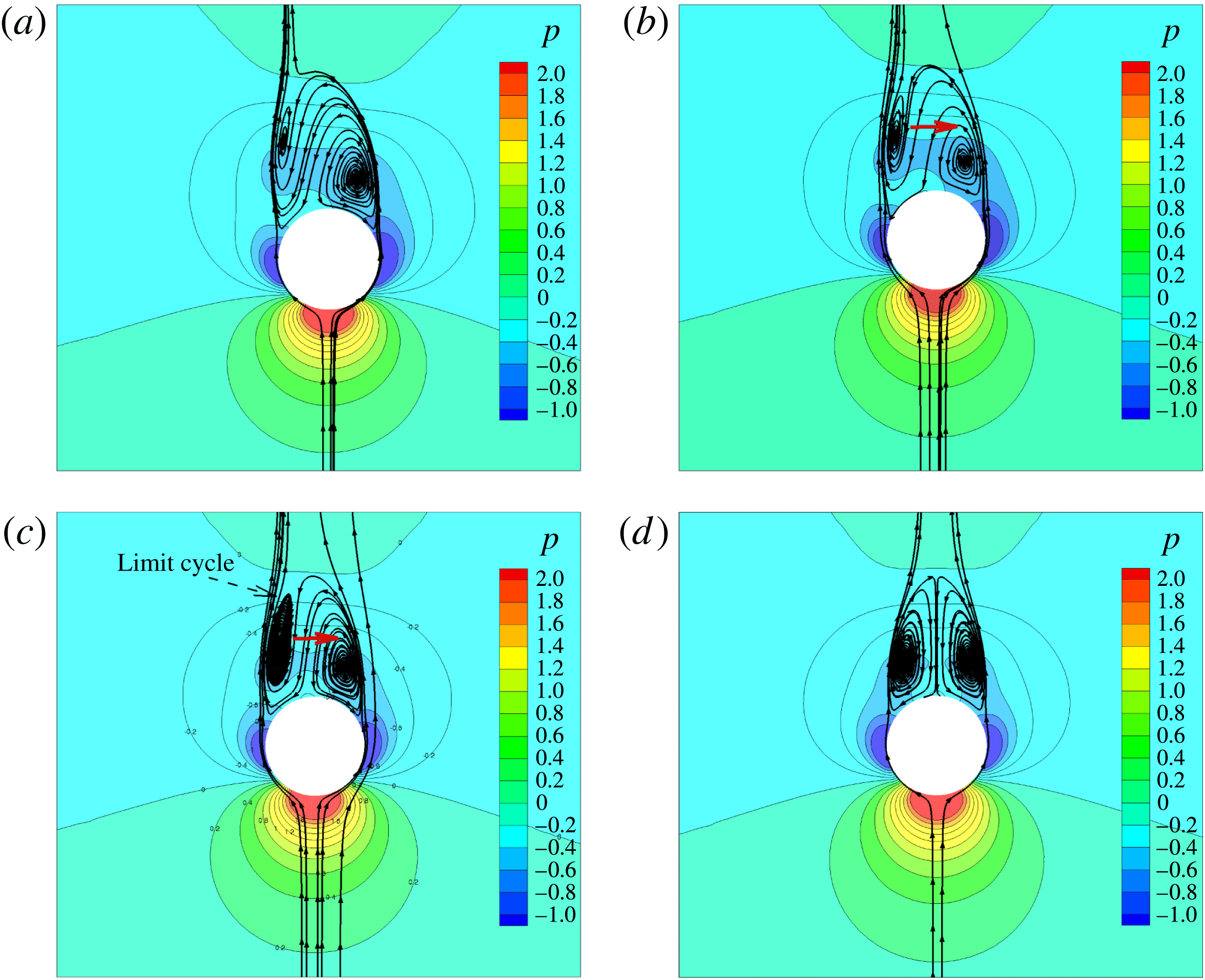
Figure 7 shows pressure contours and streamlines in the symmetric plane at
 $Re=250$
with different small interaction parameters. Since any movement non-parallel to the magnetic field will be suppressed by the Lorentz force, flows feeding the left spiral from upstream fluid and released from the right spiral are pulled to the right by the Lorentz force in figure 7(b). As the arrow represents the moving trend, these flows move to the right compared with the situation without a magnetic field. Consequently, the left spiral will grow. With an increasing interaction parameter, the left spiral will continuously grow until the sizes of the left and right spirals are identical. Figure 7(d) shows a symmetric separation bubble at
 $N=0.3$
. This indicates that the topological structure has transitioned from a steady plane symmetry into a steady axisymmetry. The disappeared non-axisymmetry also leads to a zero lift force.
Pressure contours and streamlines in the symmetric plane at
 $Re=250$
with different small interaction parameters. The arrow represents the moving trend. (a)
 $N=0$
; (b)
 $N=0.1$
; (c)
 $N=0.2$
; (d)
 $N=0.3$
.

Comparing figure 7(b,c), with the left spiral growing, the upstream fluid no longer feeds the left spiral. It seems that the left spiral is isolated in the symmetric plane. The left spiral is large enough and its head (far away from the sphere surface) is nearly open to the wake flow. So now the upstream fluid cannot feed it and spirals inward. The upstream fluid just flows around the left spiral and heads downstream. Hence the left spiral is maintained by shearing action. Now we use a dynamic and evolution-based view of the left spiral. If the left spiral does not reach a stable state, while it is initially small, the upstream fluid will feed it and it will grow to the stable state; or while it is initially large, the head of the left spiral is open to the wake flow and cannot maintain the recirculation process, which will then decrease to the stable state. So the left spiral is enclosed by a ‘limit cycle’ to which streamlines converge from both sides. The term ‘limit cycle’ was adopted in Johnson & Patel (Reference Johnson and Patel1999). This concept was used to explain the regular vortex shedding of a flow past a sphere at
 $Re=300$
, which would lead to regular temporal cycles (or limit cycles). It is noted that the limit cycle only occurs with unsteady vortex shedding flow in Johnson & Patel (Reference Johnson and Patel1999). However at the present research, it also arises at
 $Re=250$
with
 $N=0.3$
, which is a steady plane symmetric flow. Therefore, further investigation is given in the next subsection to determine whether a limit cycle also exists in the steady plane symmetric flow without a magnetic field.
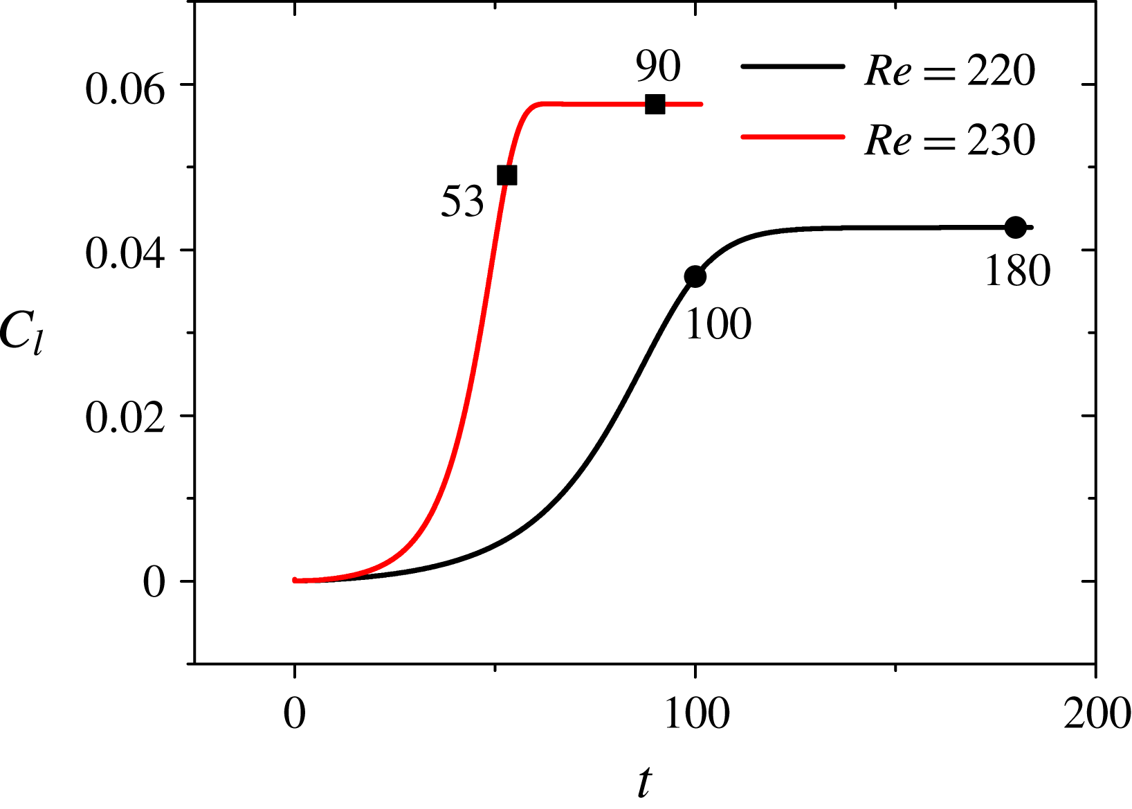
Lift coefficients with monitor points at
 $Re=220$
and
 $Re=230$
without magnetic field.

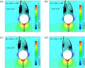
Time evolution of the pressure contours and streamlines in the symmetric plane. (a,b)
 $Re=220$
; (c,d)
 $Re=230$
.

4.2 Limit cycle
In order to find a limit cycle in the steady plane symmetric regime, time evolutions at
 $Re=220$
and
 $Re=230$
are monitored. Figure 8 shows lift coefficients with monitor points at different time instances. It can be seen that the slope of the lift coefficient at
 $Re=230$
changes sharply and goes faster into a stable state. Corresponding to four monitor points in figure 8, figure 9 shows the time evolution of the pressure contours and streamlines in the symmetric plane. The limit cycle still exists at
 $Re=220$
in the final stable state but it is no longer present at
 $Re=230$
. While the flow does not reach the final stable state at
 $Re=230$
, the limit cycle does arise at
 $t=53$
. Compared with the case at
 $Re=220$
, the larger Reynolds number represents a stronger inertial force. So the upstream fluid which flows around the left spiral has a stronger trend of moving to the left than the case at
 $Re=220$
. As a result, the left spiral is squeezed and decreases until the limit cycle is gone. Consequently, the upstream fluid feeds this left spiral and leads to a common stable state.
It is known that the steady plane symmetric wake has a range between
 $210<Re<270$
where the recirculation region behind the sphere is tilted. This tilt converts the azimuthal vorticity into a streamwise vorticity. As shown in figure 10, the streamwise vorticity is positive on one side of the sphere and negative on the opposite side. The streamwise vorticity is then carried away from the sphere surface into the wake flow. This process produces the double-threaded wake structure as seen in experiments (Magarvey & Bishop Reference Magarvey and Bishop1961) when
 $210<Re<270$
. A similar streamwise vorticity structure was also reported at
 $Re=250$
in Tomboulides & Orszag (Reference Tomboulides and Orszag2000). However, a limit cycle occurs in the symmetric plane at
 $Re=220$
while it does not at
 $Re=230$
in the final stable state. When a limit cycle is present, as shown in figure 9, the topological structure in the recirculation region is different, although these different topological structures do create the same streamwise vorticity structure or double-threaded wake structure because of the tilted recirculation region. Thus it is proposed here that there is a subregion within the range
 $210<Re<270$
which is divided by the existence or not of a limit cycle. And the point of division is between
 $Re=220$
and
 $Re=230$
based on present results.
Iso-surfaces of streamwise vorticity with
 $\unicode[STIX]{x1D714}_{z}=\pm 0.2$
. The green streamwise vorticity is positive while the blue one is negative. (a)
 $Re=220$
; (b)
 $Re=230$
.

4.3 Reversion phenomenon
Mutschke et al. (Reference Mutschke, Gerbeth, Shatrov and Tomboulides2001) investigated the influence of a streamwise magnetic field on the wake of a circular cylinder at
 $Re=200$
. An increasing magnetic field strongly changed the wake flow and as a result, wake oscillations were first weakened, eventually leading to a steady flow with attached steady bubbles. Similar results are obtained in the present research. Figure 11 shows the influence of a streamwise magnetic field on the wake structures of a sphere at
 $Re=250$
. With an increasing interaction parameter, the left spiral first grows and then becomes a limit cycle, eventually transitions to an axisymmetric state. It is interesting that figure 12 shows the same changing process but without a magnetic field. The topological structure behind the sphere at
 $Re=250$
with a certain interaction parameter corresponds to a certain case at a lower Reynolds number without a magnetic field. An example is shown in figures 11(b) and 12(b), where the topological structures are the same between the case at
 $Re=250$
with
 $N=0.1$
and the case at
 $Re=230$
without a magnetic field. We call this a ‘reversion phenomenon’.
Three-dimensional streamlines projected onto the symmetric plane at
 $Re=250$
with different small interaction parameters. (a)
 $N=0$
; (b)
 $N=0.1$
; (c)
 $N=0.2$
; (d)
 $N=0.3$
.

Three-dimensional streamlines projected onto the symmetric plane at
 $N=0$
with different Reynolds numbers. (a)
 $Re=250$
; (b)
 $Re=230$
; (c)
 $Re=220$
; (d)
 $Re=200$
.

Keep in mind that with a streamwise magnetic field, any fluid not flowing aligned with the magnetic field will be suppressed by the Lorentz force. So the Lorentz force has the trend of preventing fluid, which is between the left spiral and the right spiral in figure 11, flowing from right to left. On the other hand, the smaller Reynolds number in figure 12 means weaker inertial force and the upstream fluid, which flows around or feeds the left spiral, has a weaker trend of moving to the left. Therefore, these two situations have the same effect on the recirculation region and will gain the same topological structure behind the sphere. Alternatively, one can consider this phenomenon as a magnetic damping effect. According to Davidson (Reference Davidson2001), the Lorentz force can be reformulated as
 $\boldsymbol{J}\times \boldsymbol{B}=\unicode[STIX]{x1D735}\boldsymbol{\cdot }\unicode[STIX]{x1D749}$
, where the Maxwell stresses are
 $\unicode[STIX]{x1D70F}_{ij}=(B_{i}B_{j}/\unicode[STIX]{x1D707})-\boldsymbol{B}^{2}/2\unicode[STIX]{x1D707}\unicode[STIX]{x1D6FF}_{ij}$
. Maxwell stresses are exactly equivalent to a distributed set of viscous stresses. Following this, the kinetic energy is obtained in a straightforward way by multiplying the momentum equation with the velocity vector and performing some transformation. The dimensional form is given as
 $$\begin{eqnarray}\frac{\unicode[STIX]{x2202}\frac{1}{2}\boldsymbol{u}\boldsymbol{\cdot }\boldsymbol{u}}{\unicode[STIX]{x2202}t}+\unicode[STIX]{x1D735}\boldsymbol{\cdot }\left[\boldsymbol{u}\left(\frac{1}{2}\boldsymbol{u}\boldsymbol{\cdot }\boldsymbol{u}\right)\right]=-\frac{1}{\unicode[STIX]{x1D70C}}\unicode[STIX]{x1D735}\boldsymbol{\cdot }(p\boldsymbol{u})+\unicode[STIX]{x1D708}\unicode[STIX]{x1D735}\boldsymbol{\cdot }(\boldsymbol{u}\times \unicode[STIX]{x1D74E})-\unicode[STIX]{x1D735}\boldsymbol{\cdot }(\unicode[STIX]{x1D719}\boldsymbol{J})-\boldsymbol{J}^{2}/\unicode[STIX]{x1D70E}-\unicode[STIX]{x1D708}\unicode[STIX]{x1D74E}\boldsymbol{\cdot }\unicode[STIX]{x1D74E},\end{eqnarray}$$
where vorticity
 $\unicode[STIX]{x1D74E}=\unicode[STIX]{x1D735}\times \boldsymbol{u}$
. The last two terms represent Joule dissipation and viscous dissipation, respectively, which have the same influence on the flow. Hence, the Lorentz force action on the flow can be seen as an effective viscosity. Increasing the interaction parameter in figure 11 is equivalent to adding an effective viscosity to a hydrodynamics flow, which is equivalent to decreasing the effective Reynolds number.
4.4 Large interaction parameter situations
The small interaction parameter situation at
 $Re=250$
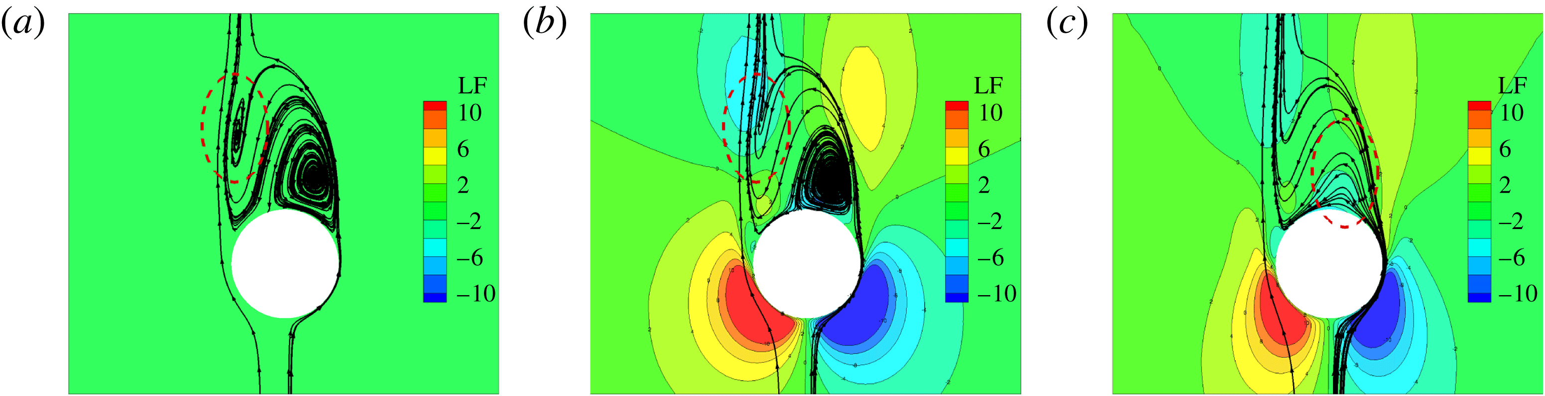
in § 4.1 shows that the magnetic field suppresses the wake and the wake structure transitions from a plane symmetry to an axisymmetry. But this is not the case for a large interaction parameter as shown in figure 6(d,e), where the small spiral is gone and the wake structure is not axisymmetric but plane symmetric. Figure 13 shows the time evolution of the Lorentz force contours and the streamlines in the symmetric plane at
 $Re=250$
with an interaction parameter of
 $N=10$
. After a large streamwise magnetic field is imposed, both the left spiral and right spiral are suppressed. Since Lorentz force is large enough, it suppresses and dismisses the left spiral directly. As shown in figure 13, a measure of the time
 $T_{i}$
after imposing a magnetic field is used. The left spiral is suppressed and becomes smaller. Then it is dismissed at
 $T_{i}=10\unicode[STIX]{x0394}t$
. At the same time, the larger right spiral is also suppressed by Lorentz force and becomes smaller with time evolution. Finally it is dismissed at
 $T_{i}=50\unicode[STIX]{x0394}t$
. It is noted that with an interaction parameter of
 $N=7$
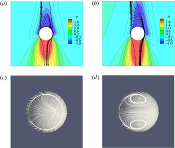
, the Lorentz force will dismiss the left spiral but just reduce the right spiral to a small one. The right spiral is still existent as shown in figure 14.
Lighthill (Reference Lighthill and Rosenhead1963) proposed the convergence of the skin friction lines to be the criterion of three-dimensional flow separation. Hence, the skin friction lines are adopted to analyse flow traces in the rear of the sphere. With a large interaction parameter, the small left spiral is dismissed. Then the upstream fluid convects from right to left because of inertia and meets with the outer upstream fluid at the left side of the sphere. Then the fluid is squeezed in the symmetric plane and flows along the azimuth direction. For a different large interaction, two types of skin friction lines are shown in figure 14. It is clearly seen that the wake remains in plane symmetry. As shown in the pressure contours and streamlines in figure 14, the meeting location side (the original left spiral side) has a higher pressure than the original right spiral side. Therefore, there is a lift force in this plane.
Time evolution of the Lorentz force contours and streamlines in the symmetric plane at
 $Re=250$
with the interaction parameter
 $N=10$
. The Lorentz force direction is from left to right. (a)
 $T_{i}=0\unicode[STIX]{x0394}t$
; (b)
 $T_{i}=10\unicode[STIX]{x0394}t$
; (c)
 $T_{i}=50\unicode[STIX]{x0394}t$
.

(a,b) Pressure contours and streamlines in the symmetric plane at
 $Re=250$
. (c,d) Skin friction lines on the sphere surface from a top view. (a,c)
 $N=7$
; (b,d)
 $N=10$
.

The time sequence of vortical structures at
 $Re=300$
during one period
 $T$
. Iso-surfaces of streamwise vorticity with
 $\unicode[STIX]{x1D714}_{z}=\pm 0.4$
. The green streamwise vorticity is positive while the blue is negative. (a)
 $t=T/4$
; (b)
 $t=2/4T$
; (c)
 $t=3/4T$
; (d)
 $t=T$
.

5 Unsteady flow affected by magnetic field
The onset of unsteadiness is known from previous studies, both experimental and numerical, to occur at a Reynolds number of approximately 270. At
 $Re=300$
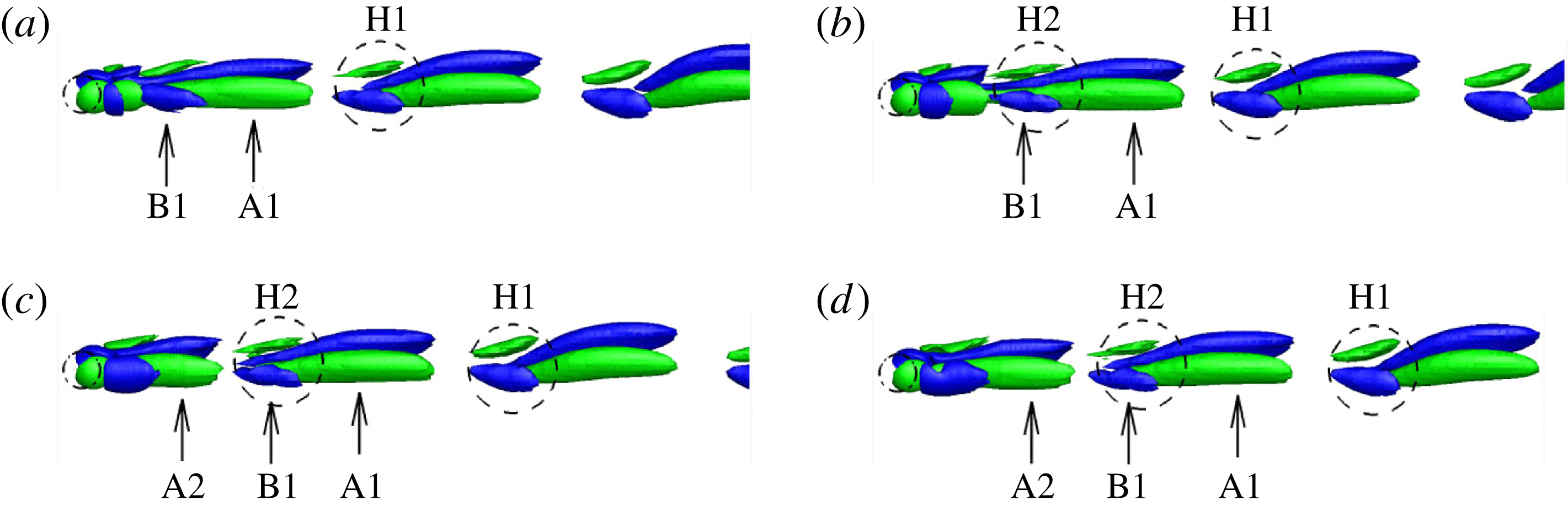
, the flow becomes unsteady and the vortices are shed periodically while the wake flow is plane symmetric. The resulting wakes are usually characterized by three-dimensional, large-scale vortical structures in the near-wake region and here they are examined by streamwise vorticity. Figure 15 shows an oblique view of the time sequence of the vortical structures’ motions during one period
 $T$
. At
 $t=T/4$
, a new vortical structure
 $B1$
is visible around the leg of the primary vortex
 $A1$
. It is suggested that this structure is induced by vortex
 $A1$
and outer flow interaction (Johnson & Patel Reference Johnson and Patel1999). Note that the vortical structures
 $A1$
and
 $B1$
have opposite directions of rotation and vortex
 $A1$
is much stronger than
 $B1$
. Later, vortex
 $B1$
develops downstream at
 $t=2/4T$
. Now a hairpin vortex
 $H2$
is evolved and shed to the downstream of the sphere. The previous hairpin vortex
 $H1$
evolved in the downstream of the sphere is also indicated in figure 15. In the following time instance
 $t=3/4T$
, the hairpin vortex
 $H2$
is completely shed to convect downstream and a new primary vortex
 $A2$
is attached to the rear of the sphere and grows. The vortex
 $A2$
grows and extends downstream at
 $t=T$
until it is strong enough to induce a new vortical structure similar to vortex
 $B1$
at
 $t=T/4$
. Then a new vortex shedding cycle begins.
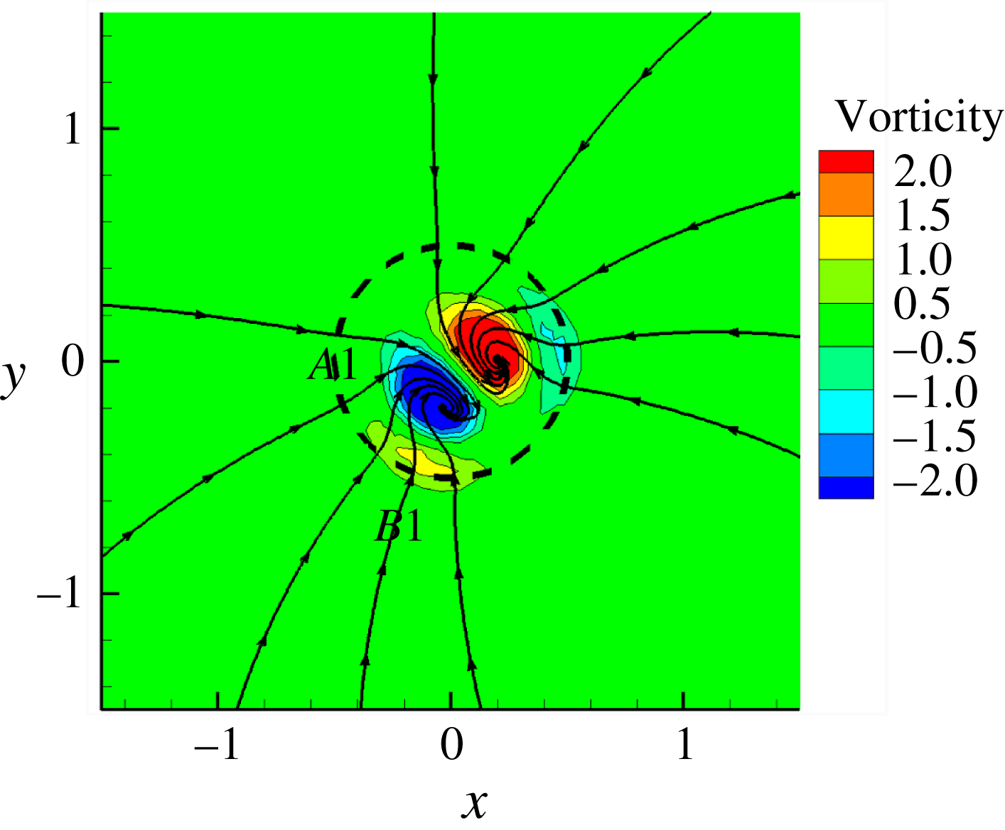
Cross-section plot of streamwise vortical structures and projective traces of cross-flow velocity.

The time sequence of vortical structures at
 $Re=300$
with
 $N=0.05$
during one period
 $T$
. Iso-surfaces of streamwise vorticity with
 $\unicode[STIX]{x1D714}_{z}=\pm 0.4$
. The green streamwise vorticity is positive while the blue is negative. (a)
 $t=T/4$
; (b)
 $t=2/4T$
; (c)
 $t=3/4T$
; (d)
 $t=T$
.

5.1 The transition from periodic to steady flow
The simulations at
 $Re=300$
with different interaction parameters are initialized with the already periodic solution of
 $Re=300$
at
 $N=0$
in figure 15. Then, a streamwise magnetic field is imposed. While the interaction number is
 $N=0.05$
, the time sequence of the vortical structures in figure 17 does not show an obvious vortex shedding, such as with the hairpin vortex in figure 15. Apparently, the wake flow is still in plane symmetry. The primary vortex grows and extends downstream and then it breaks. This process occurs periodically. Figure 16 shows a cross-section of figure 15(a) at
 $z=1.5d$
behind the sphere. The figure contains streamwise vortical structures and projective traces of cross-flow velocity. As the upstream flow approaches the clockwise rotating vortex
 $A1$
, it is turned sharply as it is dragged into the vortex
 $A1$
. Consequently, the induced motion of the outer flow is anticlockwise and a new vortical structure
 $B1$
is induced. Since any movement in this cross-section will be suppressed after the imposition of a streamwise magnetic field, both the primary vortex
 $A1$
and the induced vortex
 $B1$
will be suppressed by the Lorentz force. As a result, the intensity of the vortices will decrease, especially for vortex
 $B1$
. Therefore a scale of streamwise vorticity
 $\unicode[STIX]{x1D714}=\pm 0.4$
, which is used to visualize vortical structures, is suitable for the vortical structures in figure 15 but too large for figure 17. Actually, with a small scale, a similar new small vortex to
 $B1$
in figure 15 is induced by the primary vortex. The shedding process is also proved by the periodic lift coefficient in figure 20.
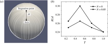
The suppression action from the Lorentz force on the vortical structure behind the sphere can be characterized by the distance between the stagnation point of skin friction lines and the axis along the sphere centre, as shown in figure 18(a). Since the stagnation point reflects the tilt of a recirculation region, the Lorentz force can cause this tilt to disappear. As is described in § 4.1, with the Lorentz force suppression, the tilt of the recirculation region at
 $Re=250$
disappears and the wake flow becomes axisymmetric. Figure 18(b) plots the time evolution of distance length
 $H$
during one period. The shedding process is similar to the situation without a magnetic field. However, it is clearly seen that the degree of tilt is greatly suppressed by the magnetic field. So the smaller tilt converts less azimuthal vorticity into the streamwise vorticity. Hence the smaller streamwise vorticity in figure 17 cannot induce a new vortex as large as the vortex
 $B1$
in figure 15. The suppression of the Lorentz force mainly acts on the recirculation region. Furthermore, the primary vortex broken in figure 17(a) develops downstream and their strength of vorticity decreases gradually with the Lorentz force suppression.
Time evolution of stagnation point of skin friction lines on the sphere surface at
 $Re=300$
during one period
 $T$
. (a) Schematic for the distance between the stagnation point and the axis along the sphere centre. (b) Time evolution of distance for different interaction parameters during one period
 $T$
.

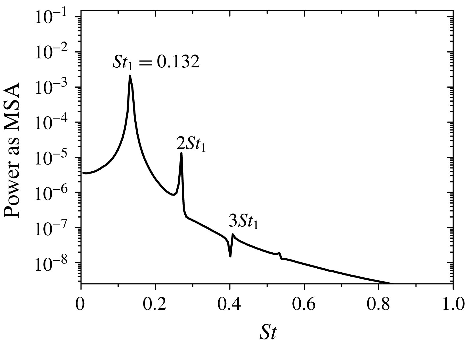
Figure 2(b) plots the power spectrum of the streamwise velocity component at the monitor point (0, 0,
 $6d$
). It shows that the shedding frequency is
 $0.136$
. The same point is monitored for
 $N=0.05$
and a similar result is plotted in figure 19. Here the shedding frequency is
 $0.132$
. However, in the numerical result of flow around a cylinder with the streamwise magnetic field, an increasing magnetic field leads to a slightly reduced shedding frequency (Mutschke et al.
Reference Mutschke, Gerbeth, Shatrov and Tomboulides2001). This effect is also shown in the experiment of Lahjomri et al. (Reference Lahjomri, Caperan and Alemany1993). The mean separation angle of a two-dimensional cylinder flow is reduced with an increasing magnetic field and the reduction should lead to a slightly smaller shedding frequency (Shatrov et al.
Reference Shatrov, Mutschke and Gerbeth1997). Johnson & Patel (Reference Johnson and Patel1999) reported that during the vortex shedding process of flow around a sphere at
 $Re=300$
, the separation angle was nearly unaffected. So after importing a magnetic field, the Lorentz force mainly has influence on the tilt of the recirculation region and the separation angle remains nearly the same. This may be the reason for almost the same shedding frequency after imposing a magnetic field. Furthermore, with the influence of a magnetic field, a stronger damping of the superharmonics can be seen in figure 19 compared to figure 2(b). The same result is reported for the cylinder case in Mutschke et al. (Reference Mutschke, Gerbeth, Shatrov and Tomboulides2001).
Power spectrum of streamwise velocity component at
 $x=0,y=0,z=6d$
at
 $Re=300$
with
 $N=0.05$
(log plot).

As shown in figure 18, the tilt of the recirculation region can be represented by the distance between the stagnation point and the axis along the sphere centre. At
 $N=0.05$
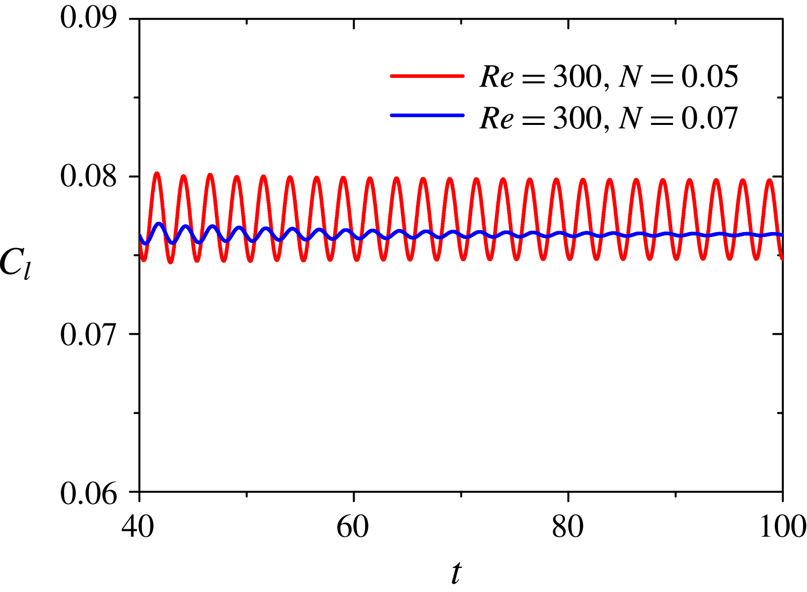
, the amplitude is very suppressed by the magnetic field. It can be predicted that with an increasing magnetic field, the amplitude will disappear and the stagnation point will be stationary. Figure 20 plots the time history of the lift coefficient. At
 $N=0.07$
, the lift coefficient is a damped oscillation compared to the case at
 $N=0.05$
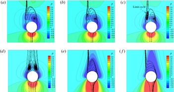
. With this larger magnetic field, the lift coefficient decays rapidly into a constant value. Now the wake flow behind the sphere is transitioned from an unsteady periodic flow to a steady flow. It is noted that the plane symmetry remains. Figure 21(a) shows its pressure contours and streamlines in the symmetric plane. It can be seen that the left small spiral is gone.
Time history of lift coefficient with damped oscillation at
 $Re=300$
with
 $N=0.07$
.

5.2 Steady flow in an increasing magnetic field and reversion phenomenon
In the section above, the periodic unsteady state is transitioned to a steady state at
 $N=0.07$
. It is noted that the wake flow is steady at
 $Re=300$
while the interaction parameter is larger than
 $0.07$
, as shown in figure 21. The topological structure behind a sphere at a steady state experiences the same structure with an increasing magnetic field at
 $Re=250$
in § 4. They both experience a larger left spiral, limit cycle, axisymmetric state and the left spiral dismissed. This phenomenon can be also seen as a reversion phenomenon that includes two aspects. One is that the topological structure in the case with a higher Reynolds number and a certain interaction parameter corresponds to a lower Reynolds number case with a certain interaction parameter. The other aspect is that the topological structure corresponds to a much lower Reynolds number case without a magnetic field. For example, the topological structure in figure 21(c) at
 $Re=300$
with
 $N=0.3$
has a limit cycle. It corresponds to the same topological structure in figure 7(c) at
 $Re=250$
with
 $N=0.2$
or figure 9 at
 $Re=220$
with
 $N=0$
.
Since the flow past a sphere at
 $Re=300$
is an unsteady periodic flow without a magnetic field, in order to check whether the different initial time instances for imposing a streamwise magnetic field influence the final steady state, four time instances of a period, as shown in figure 15, are tested at
 $N=0.5$
. All results are identical, meaning that the starting time of the magnetic field does not affect the final result and the present steady results are unique.
Pressure contours and streamlines in the symmetric plane at
 $Re=300$
with different interaction parameters. (a)
 $N=0.07$
; (b)
 $N=0.3$
; (c)
 $N=0.5$
; (d)
 $N=1$
; (e)
 $N=5$
; (f)
 $N=7$
.

6 Drag and lift coefficients
Kurose & Komori (Reference Kurose and Komori1999) applied direct numerical simulation to flow past a stationary sphere and investigated drag and lift coefficients without a magnetic field. The case with a magnetic field is different and is analysed below. The drag of the sphere had been measured in a flow of liquid sodium with a streamwise magnetic field by Yonas (Reference Yonas1967). The ranges of characteristic parameters for the experiment are
 $10^{4}<Re<25\times 10^{4}$
and
 $0<N<80$
. The research reported that for a strong magnetic field (
 $N>10$
), the drag coefficient was proportional to
 $N^{1/2}$
. A two-dimensional, incompressible MHD flow with a streamwise magnetic field around a circular cylinder was also investigated numerically using a streamfunction–vorticity formulation in Shatrov et al. (Reference Shatrov, Mutschke and Gerbeth1997). The flow was studied in the parameter range
 $Re<2000$
and
 $N<10$
. When the interaction parameter reached a certain value
 $N_{c}$
, the vortex shedding was completely suppressed and the wake flow remained steady. In their numerical results, for
 $N>N_{c}$
, the steady drag coefficient
 $C_{d}$
grew as
 $N^{1/2}$
. Based on these results, it seems that while the wake flow behind the sphere is steady and axisymmetric for a certain magnetic field, the drag coefficient
 $C_{d}$
is proportional to
 $N^{1/2}$
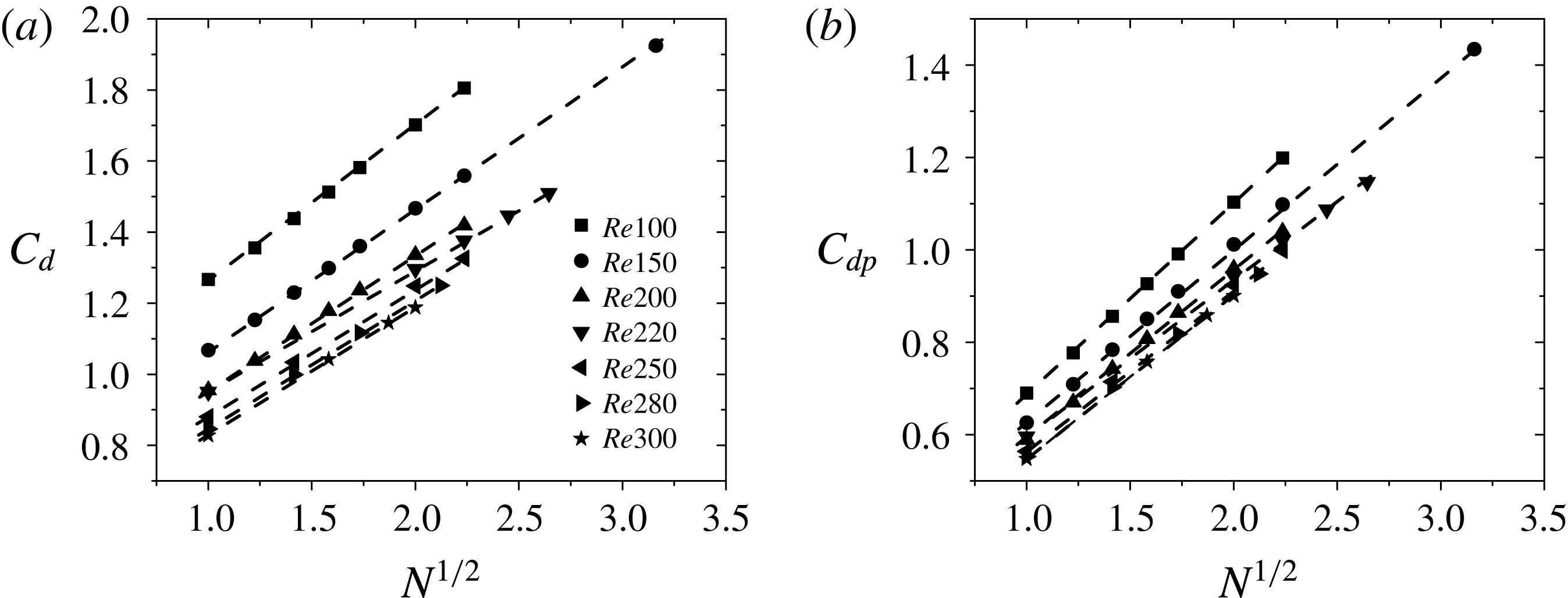
. Such a viewpoint is supported by present results. Figure 22(a) shows a linear dependence of drag coefficient
 $C_{d}$
versus
 $N^{1/2}$
. It is noted that all these data points are located at an axisymmetric state under the influence of a streamwise magnetic field when the interaction parameter
 $N>1$
. The pressure drag coefficient
 $C_{dp}$
is also plotted in figure 22(b), which shows the same linear dependence versus
 $N^{1/2}$
. It can be seen that the pressure force is the major source of the drag force.
By taking the dot product of
 $\boldsymbol{u}$
with the momentum equation, for steady and inviscid limit, one has
 $\boldsymbol{u}\boldsymbol{\cdot }\unicode[STIX]{x1D735}H=-N(\boldsymbol{u}\times \boldsymbol{B})^{2}$
(Yonas Reference Yonas1967), where
 $H$
represents the behaviour of the Bernoulli function,
 $H=p+\boldsymbol{u}^{2}/2$
. Therefore, the Bernoulli function must decrease along streamlines which are not parallel to the magnetic field. So in the stagnant regions ahead of and behind the sphere, a large pressure drop exists. As shown in figure 3, these stagnant regions mainly contribute the pressure drag force. Yonas (Reference Yonas1967) considered the immersed body to be surrounded by slender, relatively stagnant regions which were themselves separated from the outer undisturbed flow by thin dissipation layers. A perturbation technique in Childress (Reference Childress1963) suggested that the dissipation layers were of the order of
 $N^{-1/2}$
in thickness for a strong magnetic field and found a simple drag law
 $C_{d}\propto N^{1/2}$
under some assumptions.
Linear dependence of drag or pressure drag coefficient versus
 $N^{1/2}$
. (a)
 $C_{d}$
; (b)
 $C_{dp}$
.

The drag law may also be interpreted from the perspective of the energy. We set the coordinate system fixed in the centre of the sphere and make it move in the magnetic field direction with velocity
 $u_{0}$
. Since a sphere exists in the fluid, a portion of the magnetic field line is swept sideways by the lateral movement of the fluid which flows around the sphere. The lateral movement of the fluid is seen as a finite disturbance in the velocity which is not parallel to the magnetic field. The finite disturbance can propagate along the magnetic field by means of an Alfvén wave for a large interaction parameter. Such a process can carry energy away by the magnetic field (Davidson Reference Davidson2001; Moreau Reference Moreau2013). For a large interaction parameter, the energy carried away by the Alfvén wave mainly contributes to the power created from the drag force pushing the sphere movement as
 $C_{d}\sim v_{0}/u_{0}$
, where
 $v_{0}=B/(\unicode[STIX]{x1D70C}\unicode[STIX]{x1D707})^{1/2}$
is the Alfvén velocity. Furthermore, the dimensionless magnetic Reynolds number
 $R_{m}=\unicode[STIX]{x1D707}\unicode[STIX]{x1D70E}Lu_{0}$
is constant for this case. So
 $C_{d}\sim v_{0}/u_{0}R_{m}\sim B\sqrt{\unicode[STIX]{x1D70E}L}/\sqrt{\unicode[STIX]{x1D70C}u_{0}}\sim \sqrt{N}$
. Actually, with such an interpretation from the energy viewpoint, the shape of the body is negligible, meaning that the drag law can be used other cases besides that of a sphere. Indeed, a simple drag law independent of body shape was reported in experiments by Yonas (Reference Yonas1967).
Mutschke et al. (Reference Mutschke, Gerbeth, Shatrov and Tomboulides2001) reported a scenario of three-dimensional instabilities of the cylinder wake with a streamwise magnetic field. They found that with the magnetic field increased, at
 $Re=200$
the lift amplitude decreased and reached zero at a value
 $N\approx 0.3$
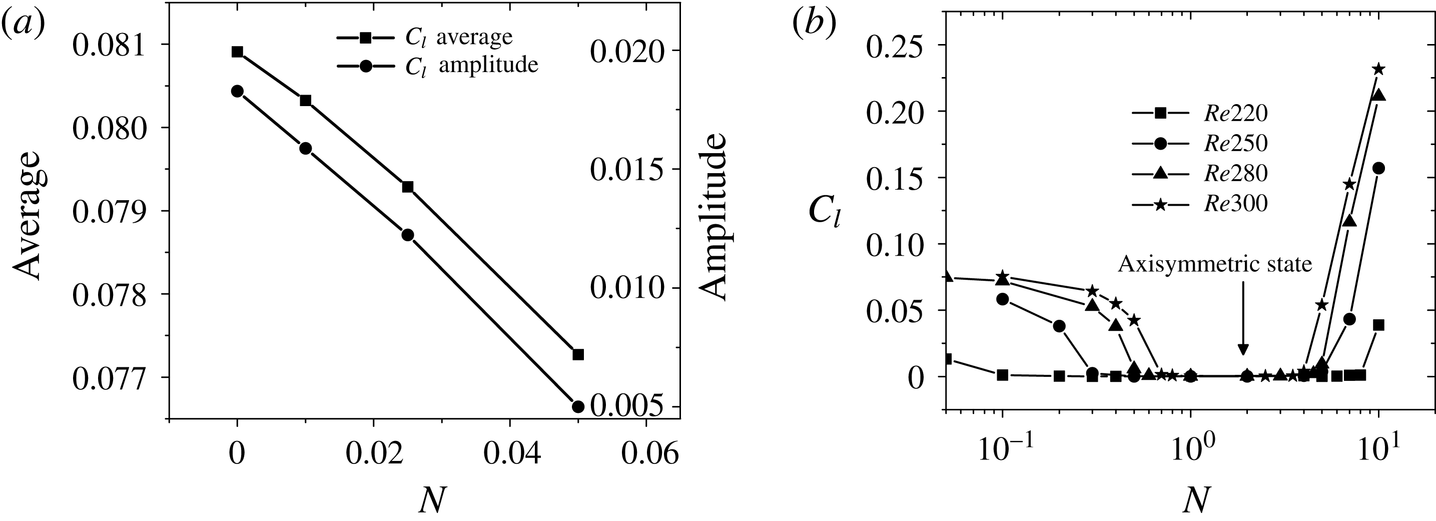
. Similar results are found in the present research. Figure 23(a) plots the average and the amplitude of the lift coefficient at
 $Re=300$
versus the interaction parameter. They both decrease with an increasing magnetic field. Furthermore, at
 $N=0.07$
, the vortex shedding is completely suppressed and the wake flow is transitioned from an unsteady periodic flow into a steady plane symmetric flow. Based on the results in the previous section (
 $Re=250$
and
 $Re=300$
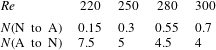
), the steady plane symmetric state will transition into an axisymmetric state with an increasing interaction parameter. And the lift coefficient corresponding to this axisymmetric state is zero. However, with a large interaction parameter, the small spiral will be dismissed and the state will transition into another kind steady plane symmetric state, as shown in figure 14 or figure 21(e,f). Since these two kinds of non-axisymmetric states are steady and have plane symmetry, a constant lift force in the symmetric plane exists. The transition to an axisymmetric state corresponds to a zero lift coefficient. Hence, the transition in a steady state with a certain magnetic field can be clearly represented by the lift coefficient, as shown in figure 23(b). A range of zero lift coefficient is shown, where the wake flow is axisymmetric, and in this range with
 $N>1$
, the drag and pressure drag coefficients are proportional to
 $N^{1/2}$
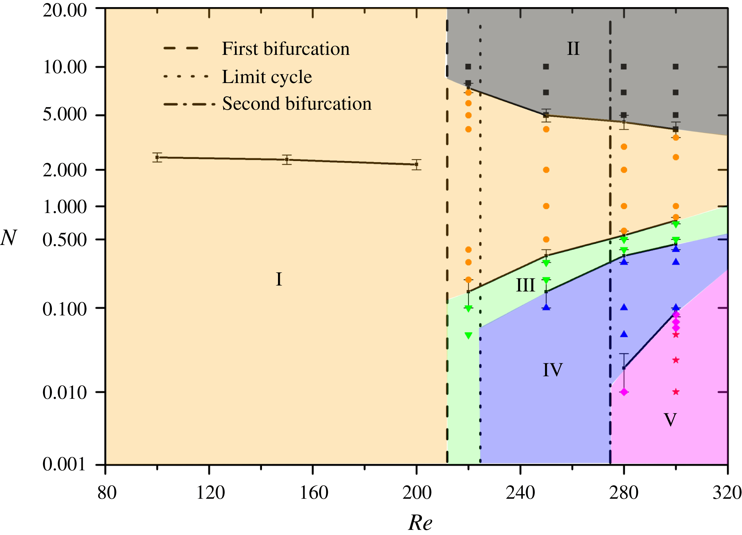
in figure 22. Detailed values of the transition points in figure 23(b) are summarized in table 2.
Lift coefficient versus the interaction parameter. (a) Unsteady part at
 $Re=300$
. (b) Steady part with different Reynolds numbers.

Map of regimes for wake patterns behind a sphere in the
 $\{N,Re\}$
plane. For the cases without a magnetic field, the dashed and dot-dashed lines represent the first bifurcation and second bifurcation, respectively. A subregion with a limit cycle is divided by the dotted line. It is located around Reynolds number 220 and 230. For the case with a magnetic field, regime I is the steady axisymmetric state with an attached separation bubble. The pattern in regime II is the steady plane symmetric with a small spiral in the recirculation region dismissed. Regimes III and IV are both steady plane symmetric with a tilt recirculation region, for which the small spiral in regime III is a limit cycle but it is fed by the upstream flow in regime IV. The last regime V is unsteady plane symmetric, for which ♢ represents a damped oscillation and
 $\star$
represents a periodic vortex shedding.

The transition points of the lift coefficient at steady state for different Reynolds numbers. N to A means a non-axisymmetric state to an axisymmetric state. A to N means an axisymmetric state to a non-axisymmetric state.

7 Summary
The present study is undertaken with the objective of numerically simulating and analysing in detail the wake structure and transition of the flow past a sphere under the influence of an imposed streamwise magnetic field, which is among the first three flow regimes, namely the steady axisymmetric flow, the steady plane symmetric flow and the unsteady periodic flow, with Reynolds number up to
 $300$
. In order to define the various wake structures and transition processes, nearly
 $100$
different cases are performed. The principal results of the present work are to give the map of regimes for wake patterns behind a sphere in the
 $\{N,Re\}$
plane, as shown in figure 24.
For the case without a magnetic field, the first bifurcation (
 $Re\approx 210$
) and second bifurcation (
 $Re\approx 270$
) are fully investigated. A range between these two bifurcations (
 $210<Re<270$
) corresponds to a steady plane symmetric wake consisting of two trailing counter-rotating vortices. The present work finds a subregion with the existence of a limit cycle in the range. And the point of division is between
 $Re=220$
and
 $Re=230$
. In this subregion, the left spiral in the tilted recirculation region is maintained by a shearing action, which is different from the one fed by the upstream fluid. As shown in figure 9, with the existence of limit cycle, the topological structures in the recirculation region are different.
For the case with a magnetic field, five wake patterns and their transitions are shown in figure 24. Regime I is the steady axisymmetric wake with an attached separation bubble. It is noted that while the Reynolds number is less than the first bifurcation, a non-monotonic behaviour in separation length or separation angle is found, which is caused by different main acting positions of the Lorentz force. A point and line plot indicating the inflection point of separation length is given in regime I. The wake pattern in regime II is steady plane symmetric. With a large interaction parameter, the small spiral in the recirculation region is dismissed while the large spiral is suppressed and is smaller or even disappears. Furthermore, its non-axisymmetry generates a non-zero lift coefficient. The other steady plane symmetric patterns consisting of double-threaded wake are in regimes III and IV. There are both small and large spirals in the tilted recirculation region; however, the small spiral in the tilted recirculation region of regime III is a limit cycle while the small spiral is fed by the upstream fluid in regime IV. The last wake pattern in regime V is unsteady plane symmetric. In this regime, the double-thread wake shows wave-like oscillations or hairpin vortices shed from the sphere. Transition processes in these five wake patterns are determined by the interaction parameter and Reynolds number. The Reynolds number determines the hydrodynamic transition, such as the first and second bifurcations or the limit cycle. The interaction parameter represents the influence of the magnetic field on the hydrodynamic wake structure. The wake will be transitioned to various patterns with an imposed streamwise magnetic field, as shown in figure 24. The transition process can also be represented by the lift coefficient, as shown in figure 23. The head and tail of the zero lift coefficient mean the transition points, for which the detailed values are given in table 2.
A so-called ‘reversion phenomenon’ is found. This means that the topological structure in a case with a higher Reynolds number and a certain interaction parameter corresponds to a lower Reynolds number case with a certain interaction parameter or a much lower Reynolds number case without a magnetic field. Furthermore, the drag coefficient is found to be proportional to
 $N^{1/2}$
in the axisymmetric state (regime I) while
 $N>1$
, which is consistent with previous experimental and numerical reports.
Acknowledgements
The authors gratefully acknowledge the support from NSFC (# 51636009 and # 51776194), and from CAS (# XDB22040201). The authors thank the anonymous reviewers for their comments, which improved the quality of the paper dramatically.