2.1 LES framework: numerical method and physical model

The governing equations for LES of incompressible viscous flow are derived by formally applying a spatial filter on the Navier–Stokes equations. These are

(2.1) $$\begin{eqnarray}\displaystyle \frac{\unicode[STIX]{x2202}\widetilde{u_{i}}}{\unicode[STIX]{x2202}t}+\frac{\unicode[STIX]{x2202}\widetilde{u_{i}}\widetilde{u_{j}}}{\unicode[STIX]{x2202}x_{j}}=-\frac{\unicode[STIX]{x2202}\tilde{p}}{\unicode[STIX]{x2202}x_{i}}+\unicode[STIX]{x1D708}\frac{\unicode[STIX]{x2202}^{2}\widetilde{u_{i}}}{\unicode[STIX]{x2202}x_{j}^{2}}-\frac{\unicode[STIX]{x2202}T_{ij}}{\unicode[STIX]{x2202}x_{j}},\quad \frac{\unicode[STIX]{x2202}\widetilde{u_{i}}}{\unicode[STIX]{x2202}x_{i}}=0. & & \displaystyle\end{eqnarray}$$

Here $x_{i}$ , $i=1,2,3$ are Cartesian coordinates with $\widetilde{u_{i}}$ the corresponding filtered velocity and $\widetilde{p}$ the filtered pressure. $T_{ij}=\widetilde{u_{i}u_{j}}-\widetilde{u_{i}}\widetilde{u_{j}}$ denotes the effect of unresolved scales on the resolved-scale motion, which is modelled via a sub-grid scale (SGS) model.

It is convenient sometimes to use $(x,y,z)$ as Cartesian coordinates with $(u,v,w)$ as the corresponding filtered velocity components. Two other coordinate systems are also utilized: the first is cylindrical coordinates ( $\unicode[STIX]{x1D703},y,r$ ) with velocity components ( $u_{\unicode[STIX]{x1D703}},u_{y},u_{r}$ ), which is useful for analysing results, while the second is general curvilinear coordinates $(\unicode[STIX]{x1D709},y,\unicode[STIX]{x1D702})$ , used for the implementation of the numerical method.

The governing LES equations are discretized on a body-fitted computational domain $(\unicode[STIX]{x1D709},y,\unicode[STIX]{x1D702})$ which is mapped from the physical domain in $(x,y,z)$ coordinates. Discretization employs a fourth-order-accurate, central-difference scheme for all terms, except the convective term, which uses a fourth-order energy-conservative scheme for the skew-symmetric form (Morinishi et al. Reference Morinishi, Lund, Vasilyev and Moin1998). For time integration, a third-order Runge–Kutta scheme is used, combined with the fractional-step method. The modified Helmholtz equation for velocity and the Poisson equation for pressure are solved with a multigrid method with line-relaxed Gauss–Seidel smoothers. The code is described in detail by Zhang et al. (Reference Zhang, Cheng, Gao, Qamar and Samtaney2015), Zhang & Samtaney (Reference Zhang and Samtaney2016) for DNS of airfoil flow and by Cheng et al. (Reference Cheng, Pullin, Samtaney, Zhang and Gao2017, Reference Cheng, Pullin and Samtaney2018) for LES of flow past non-rotating cylinder. The present implementation is identical to that described in § 2.1 of Cheng et al. (Reference Cheng, Pullin, Samtaney, Zhang and Gao2017), where outer boundary conditions and use of a sponge region to control the effect of the far wake on the near-cylinder flow are described. All LES reported here use a span-diameter ratio $L_{y}/D=3$ and an O grid of radius of $L_{r}=40D$ . The O grid is a cylinder fitted with equal grid spacing in both the azimuthal and spanwise directions but with grid stretching in the radial direction, particularly near the cylinder surface. The no-slip boundary condition at a stationary cylinder surface is here replaced by $(u_{\unicode[STIX]{x1D703}},u_{y},u_{r})=(\unicode[STIX]{x1D6FC}D/2,0,0)$ at the cylinder surface.

For LES we employ the stretched-vortex SGS model (SVM) (Misra & Pullin Reference Misra and Pullin1997; Voelkl, Pullin & Chan Reference Voelkl, Pullin and Chan2000; Chung & Pullin Reference Chung and Pullin2009), where the subgrid flow is modelled by spiral vortices (Lundgren Reference Lundgren1982) stretched by the eddies comprising the local resolved-scale flow. The implementation of the SVM is described in detail in § 2.2 of Cheng et al. (Reference Cheng, Pullin, Samtaney, Zhang and Gao2017, Reference Cheng, Pullin and Samtaney2018) and summarized presently in appendix B. The surface skin friction is obtained using a one-sided, four-point stencil defined by their equation (2.12) after first subtracting the solid-body rotation field with azimuthal speed $\unicode[STIX]{x1D6FC}r$ . The present LES is wall-resolved, meaning that the wall-normal grid size at the wall is on the order of the local viscous wall scale $u_{\unicode[STIX]{x1D70F}}/\unicode[STIX]{x1D708}$ , where $u_{\unicode[STIX]{x1D70F}}\equiv \sqrt{|\unicode[STIX]{x1D749}_{w}|/\unicode[STIX]{x1D70C}}$ is the friction velocity with $|\unicode[STIX]{x1D749}_{w}|$ the magnitude of the wall shear stress and $\unicode[STIX]{x1D70C}$ the constant fluid density. See Cheng et al. (Reference Cheng, Pullin, Samtaney, Zhang and Gao2017) for further details and also tables 1 and 2 of this paper.

2.2 LES performed

Figure 1.

Sketch of simulation geometry. (a) 3D view of the flow configuration with $(x,y,z)$ coordinates; (b) cross-section view of the cylinder with $(\unicode[STIX]{x1D703},r)$ coordinates. $\unicode[STIX]{x1D703}$ is measured in the clockwise direction with $\unicode[STIX]{x1D703}=0$ on the most windward point of the cylinder surface. $U_{\infty }$ is the free-stream speed and $\unicode[STIX]{x1D6FA}$ the (constant) angular velocity of the cylinder. The flow can be described by two dimensionless parameters: Reynolds number $Re_{D}=U_{\infty }D/\unicode[STIX]{x1D708}$ and velocity ratio $\unicode[STIX]{x1D6FC}=\unicode[STIX]{x1D6FA}D/(2U_{\infty })$ , where $\unicode[STIX]{x1D708}$ is the kinematic viscosity.

Table 1.

LES flows with $Re_{D}=6\times 10^{4}$ and varying $\unicode[STIX]{x1D6FC}$ . For all cases, the domain size is $40D$ in the radial $r$ direction and $3D$ in the spanwise $y$ direction.

Table 2.

LES flows with $Re_{D}=5\times 10^{3}$ and varying $\unicode[STIX]{x1D6FC}$ . For all cases, the domain size is $40D$ in the radial $r$ direction and $3D$ in the spanwise $y$ direction.

Table 3.

Summary of experimental data discussed in the present study.

The cylinder geometry is depicted in figure 1. In $(x,y,z)$ coordinates the free-stream velocity vector is in the positive $x$ -direction while the cylinder axis is aligned with the $y$ -axis. The cylinder rotates with dimensional angular velocity $\unicode[STIX]{x1D6FA}$ in the sense of the right-hand screw rule. The azimuthal angle $\unicode[STIX]{x1D703}$ is as shown. Here and subsequently we refer to that part of the cylinder surface instantaneously lying in $0\leqslant \unicode[STIX]{x1D703}\leqslant 180^{\circ }$ ( $z\geqslant 0$ ), where the $x$ -component of the cylinder surface speed is in the direction of the free stream as the ‘top’ or advancing part of the cylinder and that part instantaneously in $180^{\circ }\leqslant \unicode[STIX]{x1D703}<360^{\circ }$ ( $z<0$ ), where the $x$ -component of the cylinder surface speed opposes the free stream as the ‘bottom’ or retreating portion of the cylinder surface.

A summary of both experimental and simulation data from reference studies is shown in table 3, with $Re_{D}\leqslant 1.28\times 10^{5}$ . For $Re_{D}=5\times 10^{3}$ , DNS results (Aljure et al. Reference Aljure, Rodríguez, Lehmkuhl, Pérez-Segarra and Oliva2015) show that $C_{L}$ increases monotonically in the range $0<\unicode[STIX]{x1D6FC}<5$ . In experiments by Swanson (Reference Swanson1961), for flows with $3.58\times 10^{4}<Re_{D}<4.9\times 10^{4}$ , the variation of $C_{L}$ with $\unicode[STIX]{x1D6FC}$ at fixed $Re_{D}$ does not exhibit a discernible crisis in the sense of a sudden change over a small range of $\unicode[STIX]{x1D6FC}$ . For flows with higher $Re_{D}$ , $C_{L}(\unicode[STIX]{x1D6FC})$ clearly shows lift crisis behaviour (Swanson Reference Swanson1961; Takayama & Aoki Reference Takayama and Aoki2005). The experimental data of Takayama & Aoki (Reference Takayama and Aoki2005) show $C_{L}(\unicode[STIX]{x1D6FC})$ making zero crossings and becoming negative at approximately $Re_{D}\approx 1.0\times 10^{5}$ while the data of Swanson (Reference Swanson1961) shows this at $Re_{D}\approx 1.28\times 10^{5}$ . Based on the above summary, we choose $Re_{D}=5\times 10^{3}$ as a starting verification case and also to provide a reference flow behaviour with laminar boundary layers on the cylinder surface. For our main LES we choose $Re_{D}=6\times 10^{4}$ , where the lift crisis has been demonstrated experimentally (Swanson Reference Swanson1961; Takayama & Aoki Reference Takayama and Aoki2005). Most of our LES utilize $0\leqslant \unicode[STIX]{x1D6FC}\leqslant 1$ .

Numerical code verification is described in appendix A. This includes comparison with DNS results at $Re_{D}=5\times 10^{3}$ , analysis of the wall-adjacent mesh size in wall units, examination of the two-point correlation of the spanwise velocity component for evaluating the sufficiency of the chosen spanwise domain, and a mesh refinement study at $Re_{D}=6\times 10^{4}$ for $\unicode[STIX]{x1D6FC}=0.48$ and $\unicode[STIX]{x1D6FC}=0.6$ . Unless otherwise specified, the ‘average’ or ‘mean’ is defined as a combined spanwise and time average. The averaging procedure begins after some initial transient period, and spans a time window of $250$ units of $D/U_{\infty }$ for $Re_{D}=3.9\times 10^{3}$ and approximately $60$ times $D/U_{\infty }$ for $Re_{D}=6\times 10^{4}$ .

3.1 $Re_{D}=6\times 10^{4}$ : pressure coefficient $C_{p}$ and skin-friction coefficient $C_{f\unicode[STIX]{x1D703}}$

The LES performed are summarized in table 1. Figure 2 shows azimuthal profiles of the mean surface pressure coefficient $C_{p}=2(p-p_{\infty })/(\unicode[STIX]{x1D70C}U_{\infty }^{2})$ (panels a,c,e,g) and the $\unicode[STIX]{x1D703}$ component of the mean surface vector skin-friction coefficient $C_{f\unicode[STIX]{x1D703}}=2\unicode[STIX]{x1D70F}_{w,\unicode[STIX]{x1D703}}/(\unicode[STIX]{x1D70C}U_{\infty }^{2})$ (panels b,d,f,h) for $Re_{D}=6\times 10^{4}$ over a range of $\unicode[STIX]{x1D6FC}$ chosen to capture the expected lift crisis. Here $p_{\infty }$ is the free-stream pressure which is used to make sure $C_{p}=1$ at the front stagnation point. In figure 2(a), $C_{p}$ at $\unicode[STIX]{x1D6FC}=0$ shows symmetric behaviour for the top and bottom parts of the cylinder. As $\unicode[STIX]{x1D6FC}$ increases, the azimuthal symmetry about $\unicode[STIX]{x1D703}=180^{\circ }$ is broken. At $\unicode[STIX]{x1D6FC}=0.2$ , the local minimum $C_{p}$ for the top portion of the cylinder decreases while the local minimum value on the bottom part of the cylinder increases. This is a natural tendency owing to momentum conservation and should exist for all positive $\unicode[STIX]{x1D6FC}$ cases. Similar behaviour is observed for $C_{p}$ at $\unicode[STIX]{x1D6FC}=0.48$ where the local minimum value on the bottom side of the cylinder has disappeared.

Further increase in $\unicode[STIX]{x1D6FC}$ shows a quite different trend, as for example, seen in figure 2(c). For $\unicode[STIX]{x1D6FC}=0.52$ , a plateau value for $C_{p}$ has formed which persists with increasing $C_{p}$ up to $\unicode[STIX]{x1D6FC}=0.56$ . At $\unicode[STIX]{x1D6FC}=0.56$ the local minimum on the bottom side has reappeared with a more pronounced negative minimum value compared to the original value at $\unicode[STIX]{x1D6FC}=0$ . As $\unicode[STIX]{x1D6FC}$ increases further to $\unicode[STIX]{x1D6FC}=0.6$ , there is little variation in the $C_{p}$ profile on the top side of the cylinder, while for the bottom side, a yet deeper valley appears with an even more negative minimum $C_{p}$ . For larger $\unicode[STIX]{x1D6FC}=0.68,0.8,1.0$ shown in figure 2(e), the minimum $C_{p}$ on the top side of the cylinder becomes more negative as $\unicode[STIX]{x1D6FC}$ increases while the $C_{p}$ minimum on the bottom increases algebraically. The plateau value of $C_{p}\approx -0.7$ remains almost unchanged in this range of $\unicode[STIX]{x1D6FC}$ . The overall effect is that $C_{L}$ again increases with increasing $\unicode[STIX]{x1D6FC}$ . At $\unicode[STIX]{x1D6FC}=2$ in figure 2(g) the top-side minimum $C_{p}$ is strongly negative. A $C_{p}$ plateau still exists but is increased in $C_{p}$ value and shifted azimuthally towards the bottom surface of the cylinder. There is no local $C_{p}$ minimum on the bottom side.

At $\unicode[STIX]{x1D6FC}=0$ , $C_{f\unicode[STIX]{x1D703}}$ is symmetric about $\unicode[STIX]{x1D703}=180^{\circ }$ and a small secondary-separation bubble can be observed, as shown in figure 2(b). When the cylinder is rotating, the secondary-separation bubble on the top side disappears. For $\unicode[STIX]{x1D6FC}>0.2$ , the whole leeward side of the cylinder has a negative $C_{f\unicode[STIX]{x1D703}}$ plateau, where a negative value means that the skin-friction force corresponds to a thrust. When $\unicode[STIX]{x1D6FC}=0.48$ , this plateau further moves to a lower level at approximately $C_{f\unicode[STIX]{x1D703}}=0.004$ . For $\unicode[STIX]{x1D6FC}=0.48{-}0.6$ in figure 2(d), the plateau $C_{f\unicode[STIX]{x1D703}}$ remains almost constant. At $\unicode[STIX]{x1D6FC}=0.6$ , an abrupt hill appears at approximately $\unicode[STIX]{x1D703}=270^{\circ }$ and touches $C_{f\unicode[STIX]{x1D703}}=0$ . This implies the incipient appearance of a tiny mean-flow separation region. In figure 2(f), further increase of $\unicode[STIX]{x1D6FC}$ shows further decrease of the plateau $C_{f\unicode[STIX]{x1D703}}$ value and also a smoothing of the hill. Still further increase to $\unicode[STIX]{x1D6FC}=2.0$ , as shown in figure 2(h), results in a plateau at a much smaller $C_{f\unicode[STIX]{x1D703}}$ .

3.2 $Re_{D}=5\times 10^{3}$

Figure 3.

$C_{p}$ and $C_{f\unicode[STIX]{x1D703}}$ at $Re_{D}=5\times 10^{3}$ . (a,c) $C_{p}$ ; (b,d) $C_{f\unicode[STIX]{x1D703}}$ . In (a,b): ——, $\unicode[STIX]{x1D6FC}=0$ ; – – – –, $\unicode[STIX]{x1D6FC}=0.2$ ; — ⋅ —, $\unicode[STIX]{x1D6FC}=0.4$ ; — — — —, $\unicode[STIX]{x1D6FC}=0.6$ . In (c,d): — — — —, $\unicode[STIX]{x1D6FC}=0.6$ ; — ⋅ ⋅ —, $\unicode[STIX]{x1D6FC}=0.8$ ; ——, $\unicode[STIX]{x1D6FC}=1.0$ ; — ⋅ —, $\unicode[STIX]{x1D6FC}=2.0$ .

We discuss LES results at $Re_{D}=5\times 10^{3}$ as a reference. The LES performed are summarized in table 2. For $Re_{D}=5\times 10^{3}$ , the variation of both $C_{p}$ and $C_{f\unicode[STIX]{x1D703}}$ with increasing $\unicode[STIX]{x1D6FC}$ shows an almost uniform tendency in figure 3. This includes the decreasing minimum $C_{p}$ on the top side of the cylinder and the gradual disappearance of the minimum $C_{p}$ on the bottom side. The plateau $C_{p}$ remains almost unchanged for $\unicode[STIX]{x1D6FC}<1$ . The trend of $C_{f\unicode[STIX]{x1D703}}$ variation is similarly uniform, with a monotonically decreasing plateau value.

It is of interest to compare cases with different $Re_{D}$ at fixed $\unicode[STIX]{x1D6FC}$ , for example $\unicode[STIX]{x1D6FC}=2$ in figures 2(g,h) and 3(c,d), respectively. Although profiles of $C_{f\unicode[STIX]{x1D703}}$ are rather different, the azimuthal profiles of pressure coefficient are quite close. Both cases have a minimum $C_{p}\approx -6.5$ near $\unicode[STIX]{x1D703}=90^{\circ }$ , and also a peak value $C_{p}\approx 1$ at approximately $\unicode[STIX]{x1D703}=330^{\circ }$ . Since the pressure distribution on the cylinder surface contributes the dominant part of both the drag and the lift, the dependence of the drag/lift on $Re_{D}$ is quite weak for high- $\unicode[STIX]{x1D6FC}$ cases.

3.3 Lift and drag coefficients $C_{L}$ , $C_{D}$

It has been seen that the $C_{p}$ profiles for $Re_{D}=6\times 10^{4}$ in $0\leqslant \unicode[STIX]{x1D6FC}\leqslant 1$ show rather different features than for $Re_{D}=5\times 10^{3}$ . These account for the presence of the $C_{L}$ crisis for the higher $Re_{D}$ and for smaller differences in the $C_{D}-\unicode[STIX]{x1D6FC}$ variation for the two $Re_{D}$ .

3.3.1 Lift crisis of $C_{L}(Re_{D},\unicode[STIX]{x1D6FC})$

Figure 4.

Lift coefficient $C_{L}$ . (a) full scale; (b) for $0\leqslant \unicode[STIX]{x1D6FC}\leqslant 1$ . Present LES data: ▪, $Re_{D}=5\times 10^{3}$ ; ●, $Re_{D}=6\times 10^{4}$ ; ▶, $Re_{D}=6\times 10^{4}$ with fine mesh. Reference data: ▵, DNS by Aljure et al. (Reference Aljure, Rodríguez, Lehmkuhl, Pérez-Segarra and Oliva2015) at $Re_{D}=5\times 10^{3}$ ; ▿, experiments by Swanson (Reference Swanson1961) at $Re_{D}=6\times 10^{4}$ ; ○, experiments by Thom (Reference Thom1934) at $Re_{D}=5.3\times 10^{3}$ ; ▫, experiments by Carstensen et al. (Reference Carstensen, Mandviwalla, Vita and Paulsen2014).

The $C_{L}(Re_{D},\unicode[STIX]{x1D6FC})$ results for the present LES are shown in figure 4(a) over $0\leqslant \unicode[STIX]{x1D6FC}\leqslant 2$ . Here all LES results for $Re_{D}=5\times 10^{3}$ and $6\times 10^{4}$ are shown. Also shown are DNS (Aljure et al. Reference Aljure, Rodríguez, Lehmkuhl, Pérez-Segarra and Oliva2015) at $Re_{D}=5\times 10^{3}$ and experimental measurements (Thom Reference Thom1934; Swanson Reference Swanson1961; Carstensen et al. Reference Carstensen, Mandviwalla, Vita and Paulsen2014). The present LES at $Re_{D}=5\times 10^{3}$ generally agree with both DNS at the same $Re_{D}$ and also experiment at $Re_{D}=5.3\times 10^{3}$ by (Thom Reference Thom1934). The other two experiments, Swanson (Reference Swanson1961), which covers $Re_{D}=3.5\times 10^{4}$ – $3\times 10^{5}$ , and Carstensen et al. (Reference Carstensen, Mandviwalla, Vita and Paulsen2014), in the range $Re_{D}=3.2\times 10^{4}{-}9.9\times 10^{4}$ , agree with each other. Both show a small decrease from measurements at $Re_{D}=5\times 10^{3}$ . This decrease is observed in our LES results with $Re_{D}=6\times 10^{4}$ at $\unicode[STIX]{x1D6FC}=1$ , but not at higher $\unicode[STIX]{x1D6FC}$ .

A plot of $C_{L}$ versus $\unicode[STIX]{x1D6FC}$ in $0\leqslant \unicode[STIX]{x1D6FC}\leqslant 1$ is shown in figure 4(b). Here LES data at $Re_{D}=6\times 10^{4}$ , with both a fine and coarse mesh, cases ‘F’ and ‘C’ respectively of table 1, are included. The former LES are computationally expensive and were performed only at $\unicode[STIX]{x1D6FC}=0.48,0.6$ . They show good agreement with the coarser-mesh LES at these $\unicode[STIX]{x1D6FC}$ values, indicating that the coarse-mesh LES are converged. The LES $C_{L}$ shows reasonable agreement with the data by Swanson (Reference Swanson1961) for $\unicode[STIX]{x1D6FC}\leqslant 0.48$ , before the beginning of the lift crisis. While the range of $\unicode[STIX]{x1D6FC}$ spanning the $C_{L}$ dip is well captured by the LES, the magnitude of the change differs between LES and experiment. In $0.48\leqslant \unicode[STIX]{x1D6FC}\leqslant 0.6$ , the experimental data (Swanson Reference Swanson1961) show a decreases $C_{L}\sim 0.37\rightarrow 0.24$ whereas LES data from both the fine and coarse-mesh LES show $C_{L}\sim 0.4\rightarrow -0.1$ . In comparison, Kim et al. (Reference Kim, Choi, Park and Yoo2014) report experimental measurements for flow past a rotating sphere showing $C_{L}\sim 0.3\rightarrow 0.05$ over the range $\unicode[STIX]{x1D6FC}\approx 0.53{-}0.7$ at the same $Re_{D}=6\times 10^{4}$ . For higher $Re_{D}$ , up to $Re_{D}=1.8\times 10^{5}$ they find more negative local $C_{L}$ minima. The experimental studies by Swanson (Reference Swanson1961) and Takayama & Aoki (Reference Takayama and Aoki2005) give scant details of the measurement technique for $C_{L}$ and so assessment of the experimental accuracy is uncertain. The rotating sphere experiments by Kim et al. (Reference Kim, Choi, Park and Yoo2014) show a relatively strong lift crisis consistent with the trend shown by the present LES. We conclude that the magnitude of the lift crisis for a rotating cylinder as a function of $(Re_{D},\unicode[STIX]{x1D6FC})$ remains an open question.

Figure 5.

Drag coefficient $C_{D}$ . (a) Full scale; (b) for $0\leqslant \unicode[STIX]{x1D6FC}\leqslant 1$ . Symbols same as in figure 4. $\diamondsuit$ , experiments by Takayama & Aoki (Reference Takayama and Aoki2005) at $Re_{D}=6\times 10^{4}$ .

3.3.3 Time histories of $C_{L}$ and $C_{D}$

The time histories of $C_{L}$ and $C_{D}$ for rotating-cylinder flow are known to show regular shedding and a closed curve in a phase diagram of $C_{L}$ versus $C_{D}$ , as shown by Mittal & Kumar (Reference Mittal and Kumar2003) for $Re_{D}=200$ . For high-Reynolds-number flow, strong three-dimensional (3D) flow effects together with turbulent transition in the wake flow are expected to produce a more complex $C_{L}-C_{D}$ evolution.

Figure 6.

$C_{L}$ and $C_{D}$ for $Re_{D}=5\times 10^{3}$ , cases: $\unicode[STIX]{x1D6FC}=0,1.0,2.0$ . (a) Time histories of $C_{L}(T)$ , where $T=tU_{\infty }/D$ is dimensionless physical time. (b) $C_{L}{-}C_{D}$ phase diagram.

Figure 7.

$C_{L}$ and $C_{D}$ for $Re_{D}=6\times 10^{4}$ , $\unicode[STIX]{x1D6FC}=0,1.0,2.0$ . (a) Time histories of $C_{L}$ . (b) $C_{L}{-}C_{D}$ phase diagram.

In figure 6, LES results for $\unicode[STIX]{x1D6FC}=0$ , $1.0$ and $2.0$ at $Re_{D}=5\times 10^{3}$ are shown, including the $C_{L}$ evolution with time $T$ and also the $C_{L}-C_{D}$ phase diagram. Results at $\unicode[STIX]{x1D6FC}=1.0$ show a slight increase of the fluctuation magnitude in $C_{L}(t)$ compared with $\unicode[STIX]{x1D6FC}=0$ , in agreement with the trend of DNS by Aljure et al. (Reference Aljure, Rodríguez, Lehmkuhl, Pérez-Segarra and Oliva2015). At $\unicode[STIX]{x1D6FC}=2.0$ , although the vortex shedding should vanish owing to the magnification of the asymmetry, $C_{L}$ still shows robust oscillatory behaviour owing to turbulence in the far-wake flow. This can also be observed in the $C_{L}-C_{D}$ phase diagram, which shows reasonably regular structures corresponding to shedding for $\unicode[STIX]{x1D6FC}=0$ and $1.0$ , but a rather chaotic trajectory for $\unicode[STIX]{x1D6FC}=2.0$ .

In figure 7, results at $Re_{D}=6\times 10^{4}$ are shown for $\unicode[STIX]{x1D6FC}=0$ , $1.0$ and $2.0$ . For this higher $Re_{D}$ flow, $\unicode[STIX]{x1D6FC}=1.0$ is found to produce a much smaller fluctuation in $C_{L}$ than for $\unicode[STIX]{x1D6FC}=0$ . Also from the phase diagram, $\unicode[STIX]{x1D6FC}=0$ can be seen to produce regular shedding, while for $\unicode[STIX]{x1D6FC}=1.0$ and $2.0$ , strongly chaotic behaviour overwhelms the shedding and quasiperiodic behaviour is not apparent.

Figure 8.

$C_{L}$ and $C_{D}$ for $Re_{D}=6\times 10^{4}$ across the lift crisis: $\unicode[STIX]{x1D6FC}=0.48,0.6$ . (a) Time histories of $C_{L}$ . (b) $C_{L}{-}C_{D}$ phase diagram.

Figure 9.

Skin-friction lines for case at $Re_{D}=6\times 10^{4}$ . (a) $\unicode[STIX]{x1D6FC}=0.48$ ; (b) $\unicode[STIX]{x1D6FC}=0.6$ .

It is of interest to check the time-history behaviour around the lift crisis, for example, $\unicode[STIX]{x1D6FC}=0.48$ before the lift crisis and $\unicode[STIX]{x1D6FC}=0.6$ just following the lift crisis. Figure 8 shows striking differences for these cases. At $\unicode[STIX]{x1D6FC}=0.48$ there is a strong fluctuation in $C_{L}$ while for $\unicode[STIX]{x1D6FC}=0.6$ this is largely suppressed. This suppression of vortex shedding provides a useful signature of the onset of the lift crisis. In order to quantify the fluctuation behaviour of the lift/drag coefficients we compute the root-mean-square $C_{Lrms}$ and $C_{Drms}$ , of the timewise variation of $C_{L}(t)$ and $C_{D}(t)$ , respectively. Results for $Re_{D}=5\times 10^{3}$ are shown in appendix A for comparison with the DNS of Aljure et al. (Reference Aljure, Rodríguez, Lehmkuhl, Pérez-Segarra and Oliva2015). Results at $Re_{D}=6\times 10^{4}$ are listed in table 4. It can be seen that, after the lift crisis, both $C_{Lrms}$ and $C_{Drms}$ decrease to relatively low values while $C_{Lrms}$ remains nearly constant for $\unicode[STIX]{x1D6FC}\geqslant 0.6$ .

Table 4.

LES calculation of lift coefficient fluctuation $C_{Lrms}$ , and drag coefficient fluctuation $C_{Drms}$ : $Re_{D}=6\times 10^{4}$ .

4.1 Flow reorganization: the instantaneous $\boldsymbol{C}_{\boldsymbol{f}}$ vector field

Figure 10.

Skin-friction lines for case at $Re_{D}=6\times 10^{4}$ and $\unicode[STIX]{x1D6FC}=0.6$ . This shows a close-up view of the band of small-scale separation/reattachment cells. ▫, typical repelling points (local flow reattachment). ○, typical attracting points (local flow separation).

Following Cheng et al. (Reference Cheng, Pullin, Samtaney, Zhang and Gao2017), we discuss separation and reattachment events as flow near or surrounding critical points of the $\boldsymbol{C}_{\boldsymbol{f}}$ vector field on the cylinder surface. Two representative $\boldsymbol{C}_{\boldsymbol{f}}$ surface fields for $Re_{D}=6\times 10^{4}$ are shown in figure 9 for $\unicode[STIX]{x1D6FC}=0.48$ and $\unicode[STIX]{x1D6FC}=0.6$ . With $\unicode[STIX]{x1D6FC}=0.48$ , the flow attachment line, indicated by diverging $\boldsymbol{C}_{\boldsymbol{f}}$ trajectories, is seen at approximately $\unicode[STIX]{x1D703}=5^{\circ }$ . On the top side of the cylinder, the attached flow shows large-scale separation at approximately $\unicode[STIX]{x1D703}=96^{\circ }$ while on the bottom side, the attached flow does not show a focused separation line. According to Chong et al. (Reference Chong, Soria, Perry, Chacin, Cantwell and Na1998), prior to the main flow separation, there generally exists fluctuating small-scale flow reversals scattered over a finite portion of the body surface, corresponding to multiple, scattered critical points in the $\boldsymbol{C}_{\boldsymbol{f}}$ field. For $\unicode[STIX]{x1D6FC}=0.48$ , for example at $y/D=1.0$ , the flow shows critical points at approximately $\unicode[STIX]{x1D703}=264^{\circ }$ while at $y/D=2.5$ , these are present at approximately $\unicode[STIX]{x1D703}=216^{\circ }$ . This indicates that the flow is locally strongly 3D and unsteady, with the consequence that structured separation is difficult to recognize.

Figure 11.

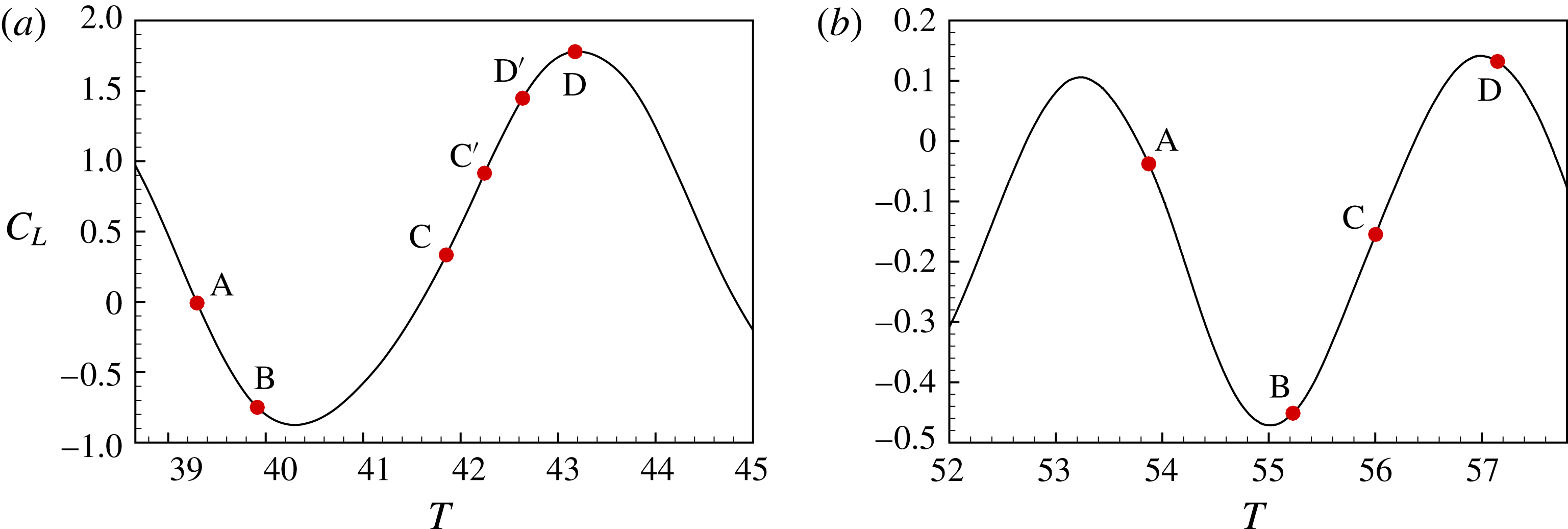
$C_{L}$ versus time for cases at $Re_{D}=6\times 10^{4}$ . (a) $\unicode[STIX]{x1D6FC}=0.48$ ; (b) $\unicode[STIX]{x1D6FC}=0.6$ . Points labelled A, B, C and D are used for comparison of flow behaviour in the shedding process. Points labelled C $^{\prime }$ and D $^{\prime }$ at $\unicode[STIX]{x1D6FC}=0.48$ are useful intermediate points.

Figure 12.

Instantaneous skin-friction lines for $\unicode[STIX]{x1D6FC}=0.48$ at $Re_{D}=6\times 10^{4}$ . (a) Instant A; (b) instant B; (c) instant C; (d) instant D. For the corresponding $C_{L}$ for each instant, see figure 11(a).

In contrast, with $\unicode[STIX]{x1D6FC}=0.6$ , the $\boldsymbol{C}_{\boldsymbol{f}}$ surface field shows a somewhat different appearance. The attachment stagnation line moves to approximately $\unicode[STIX]{x1D703}=12^{\circ }$ , while the separation line on the top side of the cylinder is still at around $\unicode[STIX]{x1D703}=96^{\circ }$ . Near $\unicode[STIX]{x1D703}=270^{\circ }$ the flow on the bottom side of the cylinder forms small-scale reversal flow cells concentrated in a zone $\unicode[STIX]{x1D703}\approx 250^{\circ }{-}280^{\circ }$ and extending across the entire span. A close-up view in $0<y/D<0.4$ is shown in figure 10. Localized flow reversals correspond to bundles of skin-friction lines appearing as separatrices connecting critical points of the $\boldsymbol{C}_{\boldsymbol{f}}$ field. Example critical points are labelled as ‘repelling’ (square symbol), where skin-friction lines diverge indicating localized reattaching flow, and as ‘attracting’ (circular symbol), where skin-friction converge implying local flow separation. A large array of roughly randomly distributed critical points exists in this region at the time instant displayed. We refer to this as an aggregation zone of small-scale, flow separation/reattachment cells. Its formation is interpreted as strong evidence of structured but distributed localized flow separation/reattachment.

4.2 Sequential $\boldsymbol{C}_{\boldsymbol{f}}(\unicode[STIX]{x1D703},y)$ portraits

In figure 11 we show the instantaneous lift coefficient $\boldsymbol{C}_{\boldsymbol{f}}(\unicode[STIX]{x1D703},y)$ at several different times during a cycle for $\unicode[STIX]{x1D6FC}=0.48$ and $0.6$ at $Re_{D}=6\times 10^{4}$ . In each panel we mark four dots which represent times at which the instantaneous $C_{f}$ fields are plotted. For the four points, point A is close to $C_{L}=0$ , point B corresponds to minimum $C_{L}$ , point C is near the midvalue between the valley and peak and point D is around the $C_{L}$ peak. For $\unicode[STIX]{x1D6FC}=0.48$ , two other instants labelled as C $^{\prime }$ and D $^{\prime }$ are shown, which will be discussed subsequently.

4.2.1 $\unicode[STIX]{x1D6FC}=0.48$

Figure 13.

Examples of ‘wash flow’ in instantaneous skin-friction lines for $\unicode[STIX]{x1D6FC}=0.48$ at $Re_{D}=6\times 10^{4}$ . (a) Close-up at instant C; (b) close-up at instant D.

Figure 14.

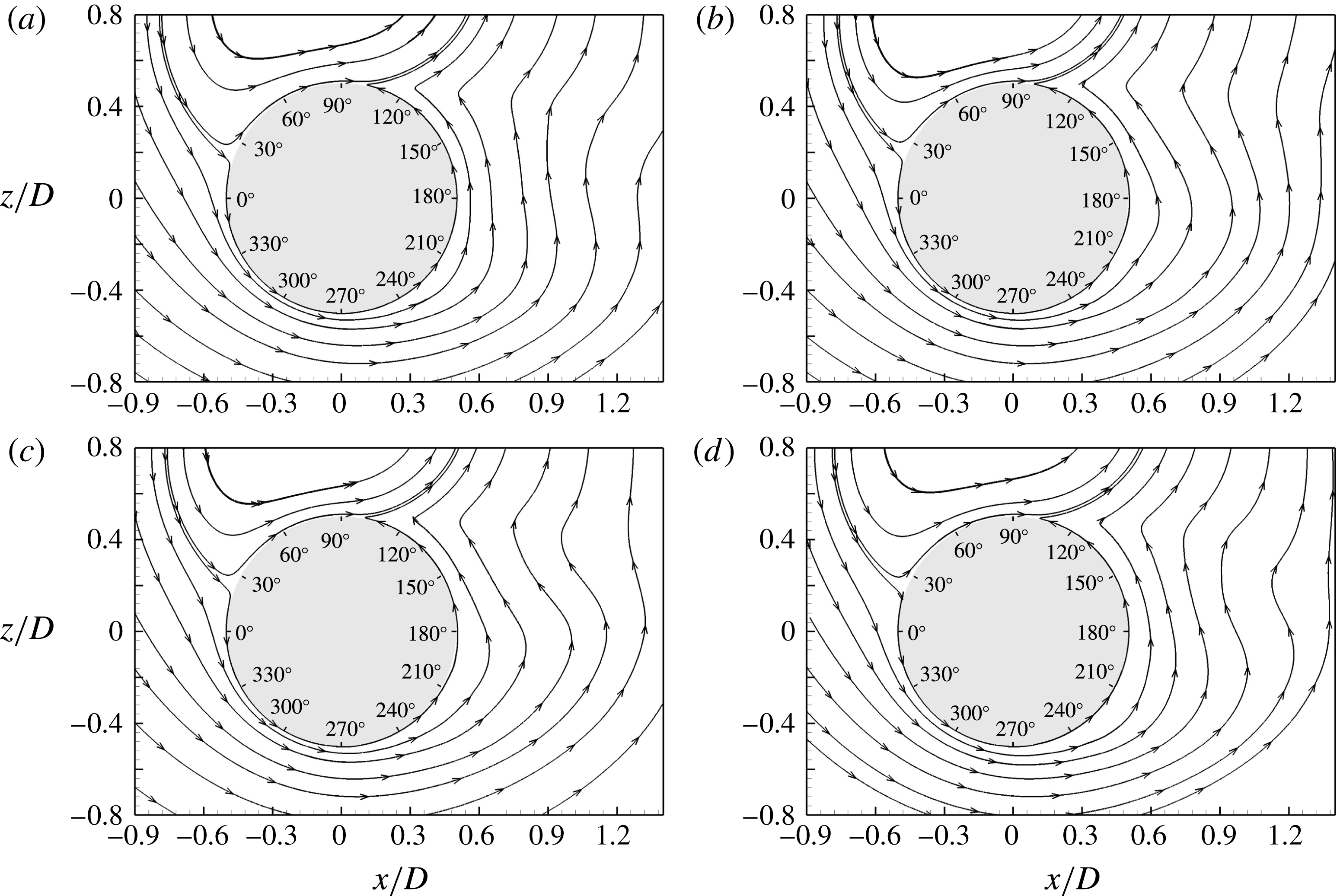
Streamlines of instantaneous spanwise-averaged fields of $\boldsymbol{u}_{\unicode[STIX]{x1D6FC}}(\unicode[STIX]{x1D703},y,r,t)$ (defined in (4.1)) for $\unicode[STIX]{x1D6FC}=0.48$ at $Re_{D}=6\times 10^{4}$ . (a) Instant A; (b) instant B; (c) instant C; (d) instant D. For the corresponding $C_{L}$ for each instant, see figure 11(a).

Figure 15.

Streamlines of instantaneous spanwise-averaged fields of $\boldsymbol{u}_{\unicode[STIX]{x1D6FC}}(\unicode[STIX]{x1D703},y,r,t)$ (defined in (4.1)) for $\unicode[STIX]{x1D6FC}=0.48$ at $Re_{D}=6\times 10^{4}$ . (a) instant C $^{\prime }$ ; (b) instant D $^{\prime }$ .

Figure 16.

Instantaneous skin-friction lines for $\unicode[STIX]{x1D6FC}=0.6$ at $Re_{D}=6\times 10^{4}$ . (a) Instant A; (b) instant B; (c) instant C; (d) instant D. For the corresponding $C_{L}$ for each instant, see figure 11(b).

For $\unicode[STIX]{x1D6FC}=0.48$ , we emphasize again that the flow on the bottom cylinder surface does not clearly show a structured pattern in the range $\unicode[STIX]{x1D703}=200^{\circ }{-}270^{\circ }$ due to its strong flow variation in the spanwise direction. In figure 12, at instant B the whole skin-friction field looks chaotic with no obvious unidirectional flow apparent at approximately $\unicode[STIX]{x1D703}=180^{\circ }$ , while for instant C a clockwise wash flow is evident at approximately $\unicode[STIX]{x1D703}=180^{\circ }$ . Among the four plots, the instant D, where $C_{L}$ shows a maximum, shows strong anticlockwise wash flow towards the top side of the cylinder at around $180^{\circ }$ . The nomenclature ‘wash flow’ is presently used to denote a sloshing and reversing but largely attached surface flow. To clarify, in figure 13, we show close-up views at instants C and D for $1.5<y/D<2.0$ . At around $\unicode[STIX]{x1D703}=180^{\circ }$ , footprints of attached clockwise directional attached flow are clearly visible at C, while at instant D, anticlockwise flow is evident. The existence of wash flow, which implies visible vortex shedding, is a feature of the flow at $\unicode[STIX]{x1D6FC}=0.48$ .

Figure 17.

Streamlines of instantaneous spanwise-averaged fields of $\boldsymbol{u}_{\unicode[STIX]{x1D6FC}}(\unicode[STIX]{x1D703},y,r,t)$ (defined in equation (4.1) for $\unicode[STIX]{x1D6FC}=0.6$ at $Re_{D}=6\times 10^{4}$ . (a) Instant A; (b) instant B; (c) instant C; (d) instant D. For the corresponding $C_{L}$ for each instant, see figure 11(b).

Figure 18.

Instantaneous, spanwise-averaged spanwise vorticity for $Re_{D}=6\times 10^{4}$ at instant of ‘C’ corresponding to figures 14(c) and 17(c). (a) $\unicode[STIX]{x1D6FC}=0.48$ ; (b) $\unicode[STIX]{x1D6FC}=0.6$ . The arrow near the colour bar indicates the ambient vorticity $\unicode[STIX]{x1D714}_{\infty }=4\unicode[STIX]{x1D6FC}U_{\infty }/D$ : $\unicode[STIX]{x1D714}_{\infty }=1.92$ for (a), $\unicode[STIX]{x1D714}_{\infty }=2.4$ for (b).

Figure 19.

An instantaneous spanwise vorticity field for $\unicode[STIX]{x1D6FC}=0.6$ at several spanwise slices.

The directional change of the wash flow provides evidence of some quasiperiodic flow behaviour. To explore this we implement a spanwise average for the four instantaneous flow fields, and plot their streamlines in figure 14. If $\boldsymbol{u}(\unicode[STIX]{x1D703},y,r,t)$ represents the full velocity field, we define spanwise-averaged, instantaneous streamlines of the modified field $\boldsymbol{u}_{\unicode[STIX]{x1D6FC}}=(u_{\unicode[STIX]{x1D6FC},\unicode[STIX]{x1D703}},u_{\unicode[STIX]{x1D6FC},y},u_{\unicode[STIX]{x1D6FC},r})$

(4.1) $$\begin{eqnarray}\boldsymbol{u}_{\unicode[STIX]{x1D6FC}}(\unicode[STIX]{x1D703},y,r,t)\equiv \boldsymbol{u}(\unicode[STIX]{x1D703},y,r,t)-\unicode[STIX]{x1D6FC}r\boldsymbol{e}_{\unicode[STIX]{x1D703}}.\end{eqnarray}$$

This is used because $\boldsymbol{u}_{\unicode[STIX]{x1D6FC}}(\unicode[STIX]{x1D703},y,r,t)=0$ on the cylinder surface, and, as a consequence, the $\boldsymbol{C}_{\boldsymbol{f}}$ portraits are in fact the limiting streamlines of $\boldsymbol{u}_{\unicode[STIX]{x1D6FC}}(\unicode[STIX]{x1D703},y,r\rightarrow D/2,t)$ on the cylinder surface, and not of $\boldsymbol{u}(\unicode[STIX]{x1D703},y,r\rightarrow D/2,t)$ . In fact this can be formulated as a general principle for bodies that are heaving and rotating with respect to a fixed laboratory frame of reference. For instant A, the streamlines clearly show two flow regions. On the top of the cylinder, the flow attaches at approximately $\unicode[STIX]{x1D703}=10^{\circ }$ and separates at approximately $\unicode[STIX]{x1D703}=100^{\circ }$ . On the cylinder bottom, the flow is also attached at approximately $10^{\circ }$ and separates at approximately $100^{\circ }$ . For instant B a small separation bubble appears in the range of $210^{\circ }<\unicode[STIX]{x1D703}<230^{\circ }$ , which corresponds to strongly 3D skin-friction lines. For instant C, this anticlockwise separation bubble increases, reflecting the strong clockwise directional wash flow evident in the skin-friction lines plot. For instant D, the near-wall flow on the bottom side of the cylinder is again fully attached, while downstream there is a clockwise-rotating vortex.

To expose detailed differences between instants C and D, we show further streamline patterns in figure 15. Figure 15(a), which corresponds to instant C $^{\prime }$ , shows a clockwise vortex at approximately $\unicode[STIX]{x1D703}=150^{\circ }$ , located off the wall and within the flow, induced by the strong shear layer. With further development, in figure 15(b) which corresponds to instant D $^{\prime }$ , we find that the wall-attached separation bubble shrinks while the new clockwise vortex increases in extent. This flow behaviour is further followed by instant D (figure 14 d), where the separation bubble disappears. This process provides a full sequence consisting of the appearance/disappearance of a pair of vortices, one anticlockwise and attached to the wall, and the other clockwise and off the wall.

Figure 20.

Skin-friction lines for $Re_{D}=6\times 10^{4}$ and $\unicode[STIX]{x1D6FC}=1.0$ . (a) Instant with minimal $C_{L}$ ; (b) instant with maximum $C_{L}$ .

Figure 21.

Skin-friction lines for $Re_{D}=6\times 10^{4}$ and $\unicode[STIX]{x1D6FC}=2.0$ .

4.3 Instantaneous pressure field

The changes in skin-friction portraits between $\unicode[STIX]{x1D6FC}=0.48$ and $\unicode[STIX]{x1D6FC}=0.6$ suggest examination of the corresponding pressure distribution on the cylinder surface. In figure 22, we show colour-coded maps of the surface pressure for $\unicode[STIX]{x1D6FC}=0.48$ , $0.6$ and $1.0$ . These show substantial changes in the location of the low-pressure region on the cylinder bottom as $\unicode[STIX]{x1D6FC}$ increases at fixed $Re_{D}$ . A low-pressure region appears at approximately $\unicode[STIX]{x1D703}=200^{\circ }$ for $\unicode[STIX]{x1D6FC}=0.48$ , shifting to around $\unicode[STIX]{x1D703}=270^{\circ }$ for $\unicode[STIX]{x1D6FC}=0.6$ . This clearly shows the flow separation behaviour across the lift crisis. For $\unicode[STIX]{x1D6FC}=1.0$ , the relative low-pressure region on the bottom part of the cylinder still resides around $\unicode[STIX]{x1D703}=270^{\circ }$ but is much weaker than for $\unicode[STIX]{x1D6FC}=0.6$ . A large low-pressure region can be seen on the top side of the cylinder. This is a common feature at all $Re_{D}$ with increasing $\unicode[STIX]{x1D6FC}$ .

A close-up view in figure 23 illustrates the relation between instantaneous pressure and identifiable features of the surface skin-friction portrait. The converging separatrices are indicative of locally separating flow, and can be seen to correspond to local, instantaneous minimal pressure, while the diverging bundles of skin-friction lines, associated with flow reattachment, tend to accumulate on patches of local maximum pressure. According to this correspondence between small-scale separation/reattachment zones, as seen in the surface skin-friction portrait, and local minima/maxima in pressure, it is reasonable to conclude that the formation of small-scale structures, perhaps in the form of near-wall recirculation eddies, results in local separation/reattachment behaviour. This is also apparent in the thin, near-wall region with concentrated vorticity, as shown in figure 19.

Figure 22.

Instantaneous pressure field on the cylinder surface for $Re_{D}=6\times 10^{4}$ . (a) $\unicode[STIX]{x1D6FC}=0.48$ ; (b) $\unicode[STIX]{x1D6FC}=0.6$ ; (c) $\unicode[STIX]{x1D6FC}=1.0$ .

Figure 23.

Instantaneous pressure field and skin-friction lines for $Re_{D}=6\times 10^{4}$ and $\unicode[STIX]{x1D6FC}=0.6$ .

4.4 Mean flow

Figure 24.

Streamlines of the mean velocity for $Re_{D}=6\times 10^{4}$ . (a) $\boldsymbol{u}_{\unicode[STIX]{x1D6FC}}(\unicode[STIX]{x1D703},y,r,t)$ field for $\unicode[STIX]{x1D6FC}=0.48$ ; (b) $\boldsymbol{u}_{\unicode[STIX]{x1D6FC}}(\unicode[STIX]{x1D703},y,r,t)$ field $\unicode[STIX]{x1D6FC}=0.6$ ; (c) $\boldsymbol{u}(\unicode[STIX]{x1D703},y,r,t)$ for $\unicode[STIX]{x1D6FC}=0.48$ ; (d) $\boldsymbol{u}(\unicode[STIX]{x1D703},y,r,t)$ field with $\unicode[STIX]{x1D6FC}=0.6$ .

In the above comparison of surface skin-friction images for cases before ( $\unicode[STIX]{x1D6FC}=0.48$ ) and after ( $\unicode[STIX]{x1D6FC}=0.6$ ) the lift crisis, we examine features of the instantaneous, spanwise-averaged flow field in order to examine local flow detail, revealing complex vortex movement for $\unicode[STIX]{x1D6FC}=0.48$ but relatively smooth flow for $\unicode[STIX]{x1D6FC}=0.6$ and above. Here we give a short description of streamlines of the mean flow at $Re_{D}=6\times 10^{4}$ , defined as a time–spanwise-averaged flow. In figure 24(a,b), we show the streamlines of the mean $\boldsymbol{u}_{\unicode[STIX]{x1D6FC}}(\unicode[STIX]{x1D703},y,r,t)$ velocity field where the two cases shows similar streamlines, all attached on the wall except for the windward attachment at around $15^{\circ }$ and separation at approximately $\unicode[STIX]{x1D703}=96^{\circ }$ . In figure 24(c,d), we plot the streamlines of the mean $\boldsymbol{u}(\unicode[STIX]{x1D703},y,r,t)$ field. The clockwise-rotating vortex bubbles in the plots should not be considered as separation bubbles. Because the cylinder is rotating, the near-wall flow always follows the wall movement and thus the clockwise vortex, which has a near-wall reversed direction, cannot reside on the surface. The flow is also characterized by an anticlockwise wall-attached bubble and an off-wall vortex. However, since we are observing the structure in the laboratory-frame velocity field, $\unicode[STIX]{x1D6FC}=0.48$ shows a smaller vortex size which extends to only $x/D\approx 0.8$ while $\unicode[STIX]{x1D6FC}=0.6$ shows a larger scale vortex which extends to $x/D\approx 1.3$ . A further detail is that, for $\unicode[STIX]{x1D6FC}=0.6$ , at around $\unicode[STIX]{x1D703}=270^{\circ }$ , the $\boldsymbol{u}(\unicode[STIX]{x1D703},y,r,t)$ flow shows a small bubble, which although still part of the wall-attached bubble, has its own low-pressure region. This is exactly the flow signature of the low- $C_{p}$ region, and in fact corresponds to the aggregation of the small-scale separation/reattachment cells on the wall discussed earlier.

5.1 PDF of skin-friction coefficient $C_{f\unicode[STIX]{x1D703}}$

To quantify the statistical features of the $C_{f\unicode[STIX]{x1D703}}$ profile, we sort $C_{f\unicode[STIX]{x1D703}}(y,t)$ over a long time frame and so construct the joint probability distribution function (PDF) $P(C_{f\unicode[STIX]{x1D703}},\unicode[STIX]{x1D703})$ , normalized such that

(5.1) $$\begin{eqnarray}\int _{-\infty }^{\infty }P(C_{f\unicode[STIX]{x1D703}},\unicode[STIX]{x1D703})\,\text{d}C_{f\unicode[STIX]{x1D703}}=1.\end{eqnarray}$$

Scatter plots depicting $P(C_{f\unicode[STIX]{x1D703}},\unicode[STIX]{x1D703})$ at $Re_{D}=6\times 10^{4}$ , with $\unicode[STIX]{x1D6FC}=0.48$ and $\unicode[STIX]{x1D6FC}=0.6$ , are shown in figure 25. Monotonic grey-scale density is used, with darker colour denoting larger (positive) values of $P(C_{f\unicode[STIX]{x1D703}},\unicode[STIX]{x1D703})$ . Comparing $P(C_{f\unicode[STIX]{x1D703}},\unicode[STIX]{x1D703})$ for the two cases at $\unicode[STIX]{x1D703}=60^{\circ }$ , where the peak value of the mean-flow $C_{f\unicode[STIX]{x1D703}}(\unicode[STIX]{x1D703})$ is observed, it can be seen that the dark region for $\unicode[STIX]{x1D6FC}=0.6$ is more concentrated, which implies weaker shedding compared to $\unicode[STIX]{x1D6FC}=0.48$ . On the bottom side of the cylinder a similar tendency can be observed at approximately $\unicode[STIX]{x1D703}=320^{\circ }$ .

Figure 25.

PDF of the skin-friction coefficient $C_{f\unicode[STIX]{x1D703}}$ for $Re_{D}=6\times 10^{4}$ . (a) $\unicode[STIX]{x1D6FC}=0.48$ ; (b)  $\unicode[STIX]{x1D6FC}=0.6$ ; (c) 3D view for $\unicode[STIX]{x1D6FC}=0.48$ ; (d) 3D view for $\unicode[STIX]{x1D6FC}=0.6$ .

Substantial differences are apparent in the plateau region – the range roughly approximately $110^{\circ }<\unicode[STIX]{x1D703}<280^{\circ }$ . For $\unicode[STIX]{x1D6FC}=0.48$ , $P(C_{f\unicode[STIX]{x1D703}},\unicode[STIX]{x1D703})$ shows broad tails in the $C_{f\unicode[STIX]{x1D703}}$ variable from $\unicode[STIX]{x1D703}=150^{\circ }$ to $210^{\circ }$ . This can be attributed to the washing flow, which changes direction gradually and slowly between up-wash and down-wash. For $\unicode[STIX]{x1D6FC}=0.6$ , a widely scattered region is found in the range $240^{\circ }<\unicode[STIX]{x1D703}<280^{\circ }$ , which covers the bottom of the cylinder. Here $P(C_{f\unicode[STIX]{x1D703}},\unicode[STIX]{x1D703})$ is broad in the $C_{f\unicode[STIX]{x1D703}}$ variable, with little dark concentration. From the previous description of the skin-friction lines, we conclude that this region is not related to the presence of washing flow. Instead, it is the result of the aggregation of small-scale separation/reattachment cells, which wrap up the critical points, resulting in chaotic local flow. For the purpose of clarity, 3D views of the two PDFs are shown in figure 25(c,d), respectively.

5.2 The $\unicode[STIX]{x1D6FE}$ parameter

Figure 26.

Sketch of the configuration of two flow regions: region I and region II. Attachment point (A) and separation point (S) are denoted.

We define the parameter $\unicode[STIX]{x1D6FE}(\unicode[STIX]{x1D703})$ as

(5.2) $$\begin{eqnarray}\unicode[STIX]{x1D6FE}(\unicode[STIX]{x1D703})=\int _{0}^{\infty }P(C_{f\unicode[STIX]{x1D703}},\unicode[STIX]{x1D703})\,\text{d}C_{f\unicode[STIX]{x1D703}}.\end{eqnarray}$$

At fixed $\unicode[STIX]{x1D703}$ , $0\leqslant \unicode[STIX]{x1D6FE}(\unicode[STIX]{x1D703})\leqslant 1$ is a measure of that total fraction of the $C_{f\unicode[STIX]{x1D703}}$ time–spanwise ensemble that are positive, i.e. $C_{f\unicode[STIX]{x1D703}}>0$ . This will now be shown to be a useful statistical metric for locally separated flow.

Table 5.

Flow features of the two regions.

The streamlines plots of $\boldsymbol{u}_{\unicode[STIX]{x1D6FC}}(r,\unicode[STIX]{x1D703},y,t)$ clearly show one attachment and one primary-separation line, which broadly divides the flow into two parts. In figure 26, these are denoted regions I and II, respectively. In the sketch, the near-wall flow in region I attaches and flows in a clockwise direction, finally separating at the denoted separation point. Hence at a given $\unicode[STIX]{x1D703}$ in region I, if the flow is always attached, then $\unicode[STIX]{x1D6FE}=1$ . Periods of statistical reversed flow at fixed $\unicode[STIX]{x1D703}$ will appear as excursions with $\unicode[STIX]{x1D6FE}(\unicode[STIX]{x1D703})<1$ . In contrast, in region II, statistically persistent attached flow at fixed $\unicode[STIX]{x1D703}$ will have $\unicode[STIX]{x1D6FE}(\unicode[STIX]{x1D703})=0$ , while reversed or backflow, that is clockwise flow, will show $\unicode[STIX]{x1D6FE}(\unicode[STIX]{x1D703})>0$ . The value $\unicode[STIX]{x1D6FE}=0.5$ is a nominal threshold (Simpson Reference Simpson1989): in region II, $\unicode[STIX]{x1D6FE}=0.5$ corresponds to instantaneous back flow 50 % of the time. Simpson (Reference Simpson1989) defines this as transitory separation. A schematic of the flow features in regions I and II is shown in table 5.

Figure 27.

$\unicode[STIX]{x1D6FE}$ for $Re_{D}=6\times 10^{4}$ . In (a): ——, $\unicode[STIX]{x1D6FC}=0$ ; — ⋅ —, $\unicode[STIX]{x1D6FC}=0.2$ , – – – –, $\unicode[STIX]{x1D6FC}=0.48$ . In (b): – – – –, $\unicode[STIX]{x1D6FC}=0.48$ ; — ⋅ ⋅ —, $\unicode[STIX]{x1D6FC}=0.52$ , — ⋅ —, $\unicode[STIX]{x1D6FC}=0.56$ , ——, $\unicode[STIX]{x1D6FC}=0.6$ . In (c): ——, $\unicode[STIX]{x1D6FC}=0.6$ ; – – – –, $\unicode[STIX]{x1D6FC}=0.68$ ; — ⋅ —, $\unicode[STIX]{x1D6FC}=0.8$ ; — ⋅ ⋅ —, $\unicode[STIX]{x1D6FC}=1.0$ . In (d): — ⋅ ⋅ —, $\unicode[STIX]{x1D6FC}=1.0$ ; – – – –, $\unicode[STIX]{x1D6FC}=2.0$ .

In figure 27, we show $\unicode[STIX]{x1D6FE}(\unicode[STIX]{x1D703})$ for all cases at $Re_{D}=6\times 10^{4}$ . Figure 27(a) shows $\unicode[STIX]{x1D6FE}(\unicode[STIX]{x1D703})$ with $\unicode[STIX]{x1D6FC}=0$ , $0.2$ and $0.48$ . For $\unicode[STIX]{x1D6FC}=0$ , the distribution is essentially symmetric about $\unicode[STIX]{x1D703}=180^{\circ }$ . For this case, $\unicode[STIX]{x1D6FE}\approx 0.5$ on the leeward side of the cylinder, indicating transitory separation. Fluctuations about $\unicode[STIX]{x1D6FE}\approx 0.5$ occur because primary separation is strongly unsteady during the shedding process. As $\unicode[STIX]{x1D6FC}$ increases, the flow is no longer symmetric. On the bottom side of the cylinder the flow tends to be attached. For $\unicode[STIX]{x1D6FC}=0.48$ , the flow in region II is generally attached, with a peak region at around $\unicode[STIX]{x1D703}=180^{\circ }$ , which is clearly associated with up-wash and down-wash flow.

In figure 27(b), four cases with $\unicode[STIX]{x1D6FC}=0.48$ , $0.52$ , $0.56$ and $0.6$ show a different tendency. With increasing $\unicode[STIX]{x1D6FC}$ , the peak at around $\unicode[STIX]{x1D703}=180^{\circ }$ weakens, while another peak emerges at approximately $\unicode[STIX]{x1D703}=270^{\circ }$ . For $\unicode[STIX]{x1D6FC}=0.6$ , that part of region II where $\unicode[STIX]{x1D6FE}\sim 0$ is focused for the most part in the zone $250^{\circ }<\unicode[STIX]{x1D703}<280^{\circ }$ , with a relatively sharp peak where $\unicode[STIX]{x1D6FE}$ is close to $0.5$ . This corresponds to the previously discussed aggregation zone of small-scale separation/reattachment cells, and indicates small-scale but localized transitory separation. With further increase of $\unicode[STIX]{x1D6FC}$ the $\unicode[STIX]{x1D6FE}(\unicode[STIX]{x1D703})$ profile does not show new features. The local peak value in region II gradually falls with increasing $\unicode[STIX]{x1D6FC}$ .

Figure 28.

$\unicode[STIX]{x1D6FE}$ for $Re_{D}=5\times 10^{3}$ . In (a): ——, $\unicode[STIX]{x1D6FC}=0$ ; – – – –, $\unicode[STIX]{x1D6FC}=0.2$ ; — ⋅ —, $\unicode[STIX]{x1D6FC}=0.4$ ; — — — —, $\unicode[STIX]{x1D6FC}=0.6$ , — ⋅ ⋅ —, $\unicode[STIX]{x1D6FC}=0.8$ . In (b): — ⋅ ⋅ —, $\unicode[STIX]{x1D6FC}=0.8$ ; — ⋅ —, $\unicode[STIX]{x1D6FC}=1.0$ , – – – –, $\unicode[STIX]{x1D6FC}=2.0$ .

It is of interest to consider the $\unicode[STIX]{x1D6FE}(\unicode[STIX]{x1D703})$ plot for the lower $Re_{D}$ flows. In figure 28 for $Re_{D}=5\times 10^{3}$ , the peak at approximately $\unicode[STIX]{x1D703}=270^{\circ }$ found at $Re_{D}=6\times 10^{4}$ at finite $\unicode[STIX]{x1D6FC}$ is not observed. Another interesting difference is the behaviour of $\unicode[STIX]{x1D6FE}(\unicode[STIX]{x1D703})$ near primary separation for $\unicode[STIX]{x1D6FC}=0$ . For $Re_{D}=6\times 10^{4}$ , $\unicode[STIX]{x1D6FE}$ only reaches $\unicode[STIX]{x1D6FE}=0.5$ , which corresponds to 50 % of back flow, implying strong shedding and corresponding movement of the primary-separation line. At $Re_{D}=5\times 10^{3}$ , $\unicode[STIX]{x1D6FE}$ extends to 100 % of back flow, reaches $\unicode[STIX]{x1D6FE}=0$ for the flow on the top side of the cylinder, and $\unicode[STIX]{x1D6FE}=1$ for the flow on the bottom side of the cylinder. This indicates that $Re_{D}=5\times 10^{3}$ has weak shedding and that the primary-separation lines show little movement.