1 Introduction
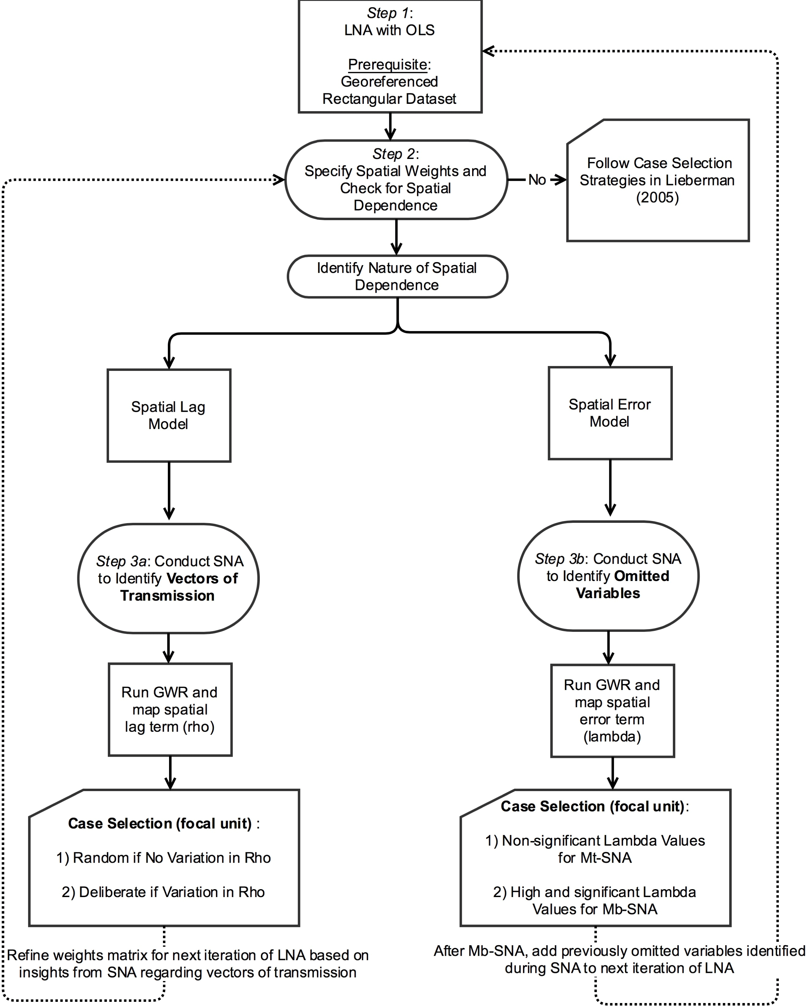
Spatial econometrics and multimethod research designs are methodological trends in the social sciences that have developed mostly in isolation of one another.Footnote 1 Spatial econometrics have been leveraged to analyze how processes of diffusion, learning, contagion, externalities, or interdependence more broadly bring about phenomena that are of interest to political science. Yet, these techniques rely on the often problematic assumption that the appropriate structure of interdependence among units, which may be based on linkages captured by geographic distance, communication flows, or travel time, is known to the researcher and can be specified ex ante. While mixed-methods designs provide opportunities to test and—if necessary—update such assumptions (Seawright Reference Seawright2016), to date strategies for case selection have been informed exclusively by unit attributes, thus limiting their ability to shed light on the nature of interdependence. In this paper we develop a framework for mixed-methods research with spatially dependent data—a framework we label “geo-nested analysis”—where insights gleaned at each step of the research process set the agenda for the next phase.Footnote 2 Our research work flow, illustrated in Figure 1, consists of three steps: (1) a nonspatial large-N analysis (LNA); (2) diagnostics of this initial model to detect spatial dependence; and (3) a small-N analysis (SNA) designed to uncover sources of dependence. If the diagnostics in step (2) indicate a spatial lag process, the small-N analysis in step (3) focuses on identifying vectors of transmission, that is, the process by which an outcome in nearby areas affects that outcome locally. Conversely, if diagnostics indicate a spatial error process, the SNA seeks to uncover spatially clustered omitted or unobserved variables, thus shedding light on “contextual effects” (King Reference King1996).
Overview of geo-nested analysis.

The key advantage of mixed-methods designs is the combination of quantitative and qualitative tools within a single unified framework. A growing literature now identifies best practices for systematically executing this multimethod integration (e.g., Seawright and Gerring Reference Seawright and Gerring2008; Humphreys and Jacobs Reference Humphreys and Jacobs2015; Nielsen Reference Nielsen2016; Seawright Reference Seawright2016). Lieberman’s (Reference Lieberman2005) article, which offers guidelines for case selection in research designs where cases for SNA are nested within a larger sample studied econometrically, was foundational for this growing literature.Footnote 3 But in line with the dominant tradition in comparative research, the assumption that the variation between units in the outcome of interest can be explained in terms of variation in unit attributes continues to underlie the LNA. This implies that units are independent of one another and that they satisfy the regression assumption of being “independent and identically distributed” (i.i.d.). Dependence among units—if considered at all—is a threat to inference but not a subject for empirical or theoretical investigation.
Yet, as Beck, Gleditsch, and Beardsley (Reference Beck, Gleditsch and Beardsley2006, 42) point out regarding many of the phenomena studied in political science, “we would expect units to be affected by what takes place in other units.” The Arab Spring—during which social protests destabilized several authoritarian regimes while other regimes responded with policies aimed at “diffusion proofing” (Koesel and Bunce Reference Koesel and Bunce2013)—is a case in point. When conceptualizing protests and regime responses as a series of isolated and unrelated events, scholars risk missing important insights about underlying causal processes (e.g., Weyland Reference Weyland2012). Other examples of interdependence stem from research on the diffusion of liberalism (e.g., Brinks and Coppedge Reference Brinks and Coppedge2006; Simmons et al. 2008), institutions (e.g., Graham, Shipan, and Volden Reference Graham, Shipan and Volden2013; Ingram Reference Ingram2016a,Reference Ingramb), norms (e.g., Hilbink Reference Hilbink2012; Ingram Reference Ingram2016c), political behavior (e.g., Huckfeldt and Sprague Reference Huckfeldt and Sprague1992), and violence (e.g., Tolnay, Deane, and Beck Reference Tolnay, Deane and Beck1996; Dube, Dube, and García-Ponce Reference Dube, Dube and García-Ponce2013).
For research using nested analysis, the spatial dependence of data presents two problems. First, nested designs are unable to answer substantive questions about the nature of interdependence among units as such questions are beyond the scope of the initial LNA. Thus, how phenomena like protest, democracy, voting, violence, or policies spread among units, or why they remain contained to specific areas, cannot be studied. Second, if the SNA identifies diffusion, transfer, spillover, learning, or other interdependence among units as relevant causal mechanisms (Shipan and Volden Reference Shipan and Volden2008), LNA and SNA become disconnected. Indeed, the more evidence of cross-unit interdependence revealed in the SNA, the more likely that the LNA is misspecified. The key promise of nested research designs “that both LNA and SNA can inform each other” and that “the analytic payoff is greater than the sum of the parts” (Lieberman Reference Lieberman2005, 436) then no longer holds. By untangling the spatial process more thoroughly than would be possible with quantitative or qualitative tools alone, geo-nested analysis offers scholars leverage to answer questions that have remained beyond the scope of systematic mixed-methods designs.
The contribution of geo-nested analysis is thus twofold. The framework: (1) enables systematic investigation of new types of questions about the nature of interdependence; and (2) by offering a strategy for explicitly integrating and triangulating evidence from quantitative and qualitative tools, places mixed-methods research designs investigating interdependence on firmer ground.
We proceed as follows. In the next section, we explain the challenge spatial dependence poses for traditional nested analysis and situate our contribution in the literature on mixed methods. We also introduce the conceptual language of spatial analysis and highlight how and why adding an SNA can improve on spatial-econometric analysis conducted in isolation. From there, we develop our framework for geo-nested analysis and walk through the steps of the research process. To illustrate these steps, we draw on the social science literature on violence, a field in which the analysis of spatial effects has been particularly fruitful. More specifically, we follow the steps of our framework with data from a seminal study of homicide rates in the United States (Baller et al. Reference Baller, Anselin, Messner, Deane and Hawkins2001). We chose this example for three reasons. First, the data for this study are publicly available and used elsewhere in the methods literature on spatial analysis to illustrate key techniques (e.g., Anselin and Rey Reference Anselin and Rey2014). Second, while Baller et al.’s analysis remains one of the preeminent examples of spatial analysis in the social sciences, the authors explicitly acknowledge uncertainties, inbuilt assumptions, and limitations—transparency that allows us to apply our framework to a real-life research example. Third, case selection strategies in our framework depend on the type of spatial dependence encountered, since different types of dependence raise distinct questions to be answered during the SNA phase of the research. While models that assume a spatial lag process challenge researchers to identify the actual vectors of transmission, a spatial error process highlights the need to uncover spatially clustered omitted variables. The Baller et al. example contains different types of spatial dependence, with homicide rates in the South following a diffusion pattern and evidence for contextual effects in the rest of the country. It is therefore a particularly rich example for illustrating different paths in the research flow of geo-nested analysis.
2 Case Selection in Space: Incorporating Dependence in Nested Analysis
Lieberman’s (Reference Lieberman2005) nested approach entails beginning the analysis with a preliminary LNA, critically assessing the robustness of the obtained results and then—depending on the outcome—proceeding either with a “Model-testing Small-N Analysis” (Mt-SNA) or a “Model-building Small-N Analysis” (Mb-SNA). Two central tenets of Lieberman’s approach are particularly relevant to the framework we develop in this paper. The first is the use of regression diagnostics for selecting promising cases for in-depth study. The second is the commitment to an iterative research process where insights gleaned at each step set the agenda for subsequent steps. Where Lieberman’s framework distinguishes between a model-testing pathway and a model-building pathway based on the robustness of the results of the quantitative model, however, we encourage mixed-method scholars to retain the commitment to testing and—if necessary—updating of LNA assumptions throughout the research cycle. Whenever there is evidence of spatial dependence, we argue, scholars should conceive of the SNA as an opportunity for hypothesis generation, model building, and improvement.Footnote 4 We retain the term “nested” in our approach because the cases selected for qualitative analysis are nested (i.e., embedded) within the same sample that is first analyzed econometrically. Even though we embrace the positivist commitment to causal inference, we therefore do not prescribe a deductive template focused primarily on hypothesis testing. Rather, our framework offers guidelines for integrating insights from quantitative and qualitative tools and for systematically and transparently refining theoretically grounded arguments (Collier, Brady, and Seawright Reference Collier, Brady, Seawright, Brady and Collier2004; Yom Reference Yom2015).
Previous guidelines for conducting nested analysis, as explained above, encounter trouble when data are spatially dependent. At the outset, it is therefore helpful to briefly explain what spatial dependence is and why it matters in the context of nested analysis. While no quantitative analysis in political science using time-series data can afford to ignore concerns about serial correlation, the issue of spatial autocorrelation in cross-sectional analysis has thus far received comparatively little attention.Footnote 5 When comparing spatial units like countries, provinces, or counties without considering the possibility of spatial dependence, scholars are in effect assuming that neighborhood and location do not matter and that units are spatially independent.Footnote 6 This is a strong assumption, probably one many scholars would be uncomfortable making explicitly. Indeed, cross-national as well as subnational quantitative analyses frequently include geographic dummy variables, implicitly acknowledging that—in addition to the variables included in the model—there are territorially specific omitted variables. In studies of violence and homicide rates in the United States, for instance, a dummy for the South is frequently included (e.g., Land, McCall, and Cohen Reference Land, McCall and Cohen1990), similar to the practice in comparative politics of incorporating regional dummies or scope exclusions (Ahram Reference Ahram2011). While such dummies often turn out to be significant, what this means substantively or theoretically is rarely explored. For this reason, Lieberman (Reference Lieberman2005, 438) cautions against the inclusion of geographic dummy variables as they “are likely to soak up some of the cross-country variance, leaving less to be explained in the SNA, but in the absence of good theory, such controls weigh against the nested approach, which aims to answer the very question of why groups of countries might vary in systematic ways” (see also Deaton Reference Deaton2010; Bell and Jones Reference Bell and Jones2015).
Lieberman, in effect, argues that geographic dummies reflect variables to be revealed during the SNA that, once identified, can be leveraged to improve the quantitative model. This is in line with Przeworski and Teune’s (Reference Przeworski and Teune1970) call to replace “proper names” with theoretically meaningful variables, and with King’s (Reference King1996, 160) commitment to show that “context” should not matter in political science analyses, i.e., that the charge of social scientists is to clarify the content of “context.” Indeed, regional dummies or contextual explanations can be seen as placeholders for variables we still need to uncover. The realization that a causal relationship plays out differently across space should not be considered the end point of analysis, but the starting point for further investigation to identify the factors underlying this contextual effect. Yet, while including undertheorized dummy variables is undesirable for the reasons outlined by Lieberman, ignoring space during the LNA runs the risk of beginning with a misspecified model. Rather than relying on geographic dummies, more explicit attention to the existence and nature of spatial dependence at the stage of a preliminary LNA can improve the research design and have multiple salutary effects, including improving existing theories and generating new ones.
In spatial econometrics, “rather than considering N observations as independent pieces of information, they are conceptualized as a single realization of a process” (Anselin and Bera Reference Anselin, Bera, Ullah and Giles1998, 252). Spatial dependence can be a threat to inference if it is not modeled adequately. Akin to problems created by omitted variable bias, coefficients can become biased and inconsistent if spatial autocorrelation is ignored (Anselin and Rey Reference Anselin and Rey2014, 105). A preliminary LNA that fails to consider spatial dependence where it exists is thus unlikely to yield “robust and satisfactory results” and will most likely lead to a “model-building Small-N Analysis” (Mb-SNA). Researchers may find this inefficient as information contained in the data about the structure of spatial dependence has not been leveraged. In the worst case scenario, the researcher begins with an Mb-SNA but has insufficient guidance to uncover the omitted variables and is then forced to end the analysis without a satisfactory answer (Lieberman’s “scenario IV”). Considering the spatial dependence in the data during the preliminary LNA gives the researcher greater guidance, not only because it avoids model misspecification, but because doing so indicates how unmeasured factors are clustered in space. This is valuable information that can be leveraged when selecting cases for SNA.
This argument for considering spatial dependence during the preliminary LNA remains in line with the practice of comparative research to find the primary explanatory factors of an outcome of interest within the unit where the outcome is observed. But, as noted in the introduction, for many phenomena studied in political science, “we would expect units to be affected by what takes place in other units” (Beck et al. Reference Beck, Gleditsch and Beardsley2006, 42). Yet, we often do not know how phenomena of interest spread from one unit to another. A more conscious consideration of spatial dependence is therefore not only about preventing quantitative analyses from getting wrong or incomplete answers to well-established questions, but about the ability to explore different types of questions (Harbers and Ingram Reference Harbers and Ingramn.d.). Understood in this way, the dependent structure in the data becomes a research topic in and of itself—one that can benefit from the systematic combination of quantitative and qualitative tools.
Adopting a spatial perspective requires researchers to re-conceptualize their understanding of the object of study during the SNA phase. Gerring (Reference Gerring2007, 19) defines a case as a “spatially delimited phenomenon (a unit) observed at a single point in time or over some period of time.” Lieberman (Reference Lieberman2005, 440) states that the move from the LNA to the SNA phase entails a shift from “dataset observations” to thicker, more heterogeneous “causal-process observations” (Collier et al. Reference Collier, Brady, Seawright, Brady and Collier2004). If observations during the LNA are countries, one or two might be selected for detailed study and analyzed over longer stretches of time to tease out causal mechanisms. For example, following Lieberman (Reference Lieberman2005), Ingram (Reference Ingram2016a) conducts a quantitative analysis of subnational judicial empowerment across states in two countries, followed by an in-depth analysis of three state-level case studies in each country. In geo-nested analysis, where data are spatially dependent, examining individual units, even in detail, is insufficient. By definition, spatial analysis focuses on the interdependence of units. Therefore, a “case” for the SNA is better conceptualized as a set of units: a focal unit (e.g., county, city, neighborhood or other unit depending on the research question and theory) and the neighboring units with which it is connected.
In sum, if spatial dependence exists in the data, geo-nested analysis has advantages over both nonspatial nested analysis and nonnested spatial analysis. We now turn to how space may be considered more explicitly and the steps in our proposed framework for geo-nested analysis.
3 Conducting Geo-Nested Analysis
While our geo-nested framework assumes an initial sequence from LNA to SNA, we readily acknowledge that most research does not proceed in a simple, linear fashion; the process is frequently iterative, with each stage informing and improving the next as theoretical hunches and intuitions develop into fully specified causal models and mechanisms (Yom Reference Yom2015). Although nested designs may be both “regression-based” and “case study-based” (Rohlfing Reference Rohlfing2008), we begin with the same idealized sequence from LNA to SNA used by Lieberman to streamline our discussion. The starting point of analysis is thus a rectangular dataset. But departing from Lieberman, our data need to be geo-referenced, that is, observations must be associated with locations in physical space.
Our discussion of specification searches and diagnostics during the LNA phase builds on Anselin and Rey (Reference Anselin and Rey2014).Footnote 7 While we highlight the main steps involved in specifying a spatial model, we refer readers looking for a more thorough discussion of diagnostics and models to texts on spatial econometrics (e.g., Anselin Reference Anselin1988; Anselin and Rey Reference Anselin and Rey2014; Darmofal Reference Darmofal2015). Throughout, we draw on an extended example of homicide rates at the county level in the United States (Baller et al. Reference Baller, Anselin, Messner, Deane and Hawkins2001).
3.1 Step 1: OLS regression with theoretically relevant variables
The construction of the rectangular dataset for the initial OLS requires the researcher to choose the spatial scale for analysis. In some instances, the appropriate scale may be obvious. To analyze welfare policies in American states, the jurisdictions making the policy decisions, i.e., states, are most likely the relevant units (Berry, Fording, and Hanson Reference Berry, Fording and Hanson2003). Often, however, the phenomenon of interest is studied at some level of aggregation and different types of aggregation are possible. For instance, violent conflict has been studied at the country level (Fearon and Laitin Reference Fearon and Laitin2003), the province level (Østby, Nordås, and Ketil Rød Reference Østby, Nordås and Ketil Rød2009; Fjelde and von Uexkull Reference Fjelde and von Uexkull2012), and at the level of grid cells (Pierskalla and Hollenbach Reference Pierskalla and Hollenbach2013).Footnote 8 The choice of scale, and associated concerns about the modifiable areal unit problem (MAUP), have received considerable attention in the literature on spatial analysis (e.g., Anselin Reference Anselin1988). Briefly, if the spatial scale is too large, the researcher is unable to detect diffusion or contextual effects even where they exist. Moreover, over-aggregation may create an ecological inference problem by obscuring relevant variation at lower levels (King Reference King1997). Scaling down, however, can be equally problematic. If the units are too small, the researcher will observe spatial autocorrelation that is neither theoretically meaningful nor substantively interesting, but which exists purely because the appropriate unit of analysis was artificially cut up into smaller pieces. The problem of identifying the appropriate scale is by no means unique to spatial analysis, but arises whenever an outcome is studied at some level of aggregation. To minimize the risk of misspecification during the LNA phase, explicit attention to the scale of analysis is needed at an early stage in the research process.
The choice for a specific spatial scale is often guided by a combination of theory and pragmatism (Soifer Reference Soifern.d.). In their analysis of homicide rates, Baller et al. recognize that “counties are arbitrary units of analysis”; the “selection of the unit of analysis should ideally be determined by theoretical considerations, but in practice, data availability imposes severe constraints” (Baller et al. Reference Baller, Anselin, Messner, Deane and Hawkins2001, 568–569; also Darmofal Reference Darmofal2006, 126). We would add that even if data are available at multiple scales, theory may offer insufficient guidance to dispose of the issue. Scholars are therefore likely to rely on a combination of theoretical hunches and case knowledge when deciding at which scale to collect their data. We encourage researchers to make their considerations explicit, to do robustness tests, be open to revisiting the issue at a later stage during the research process, and to collect data at the lowest level of aggregation possible, acknowledging that it is easier to aggregate up from collected data than to collect new data in order to disaggregate.
Once the dataset has been constructed, the first step in geo-nested analysis is to begin with a preliminary LNA with theoretically relevant variables. At this stage, researchers should ensure the model reflects the theoretical “state of the art” and that it is properly specified.Footnote 9 In our homicide example, the explanatory variables come from an influential study of homicide rates (Land et al. Reference Land, McCall and Cohen1990). Baller et al. (Reference Baller, Anselin, Messner, Deane and Hawkins2001) use Land et al.’s specification as their baseline model but seek to identify and incorporate spatial effects.Footnote 10 The dependent variable of the analysis is homicide rate (per 100,000 people); key predictors are resource deprivation (rd90), population structure (ps90), median age (ma90), divorce rate (dv90), unemployment rate (ue90), and a dummy variable for the southern part of the country (south). Baller et al. begin with the following baseline model:
 $$\begin{eqnarray}y_{i}=\mathop{\sum }_{k}x_{ki}\unicode[STIX]{x1D6FD}_{k}+u_{i}.\end{eqnarray}$$
In the model,
 $y$
is the outcome of interest (homicide rates) at location
 $i$
,
 $x$
is an
 $i\times k$
matrix of
 $k$
independent variables for each location
 $i$
,
 $\unicode[STIX]{x1D6FD}$
is a
 $k\times 1$
vector of coefficients for each of the independent variables, and
 $u$
is a normally distributed random error term for each location
 $i$
. Note that in the original baseline model, the matrix
 $x$
includes a regional dummy variable. In this basic, global model, there is a single coefficient
 $\unicode[STIX]{x1D6FD}$
for each predictor across the entire sample of geographic units. That is, each coefficient is uniform or stationary across the entire space, assuming that the same relationship holds in unit 1 as in unit 3,085.
As outlined above, research on violence in the U.S. has generally included a dummy variable for the South. But despite research on a southern culture of violence (e.g., Nisbett Reference Nisbett1993), a well-developed theoretical explanation for its significance is still lacking (Baller et al. Reference Baller, Anselin, Messner, Deane and Hawkins2001). Following Lieberman, we run the baseline model again, but without the regional dummy.
3.2 Step 2: Identify existence and nature of spatial dependence
The next step is to determine the presence and nature of remaining spatial autocorrelation once the covariates in the model have been considered. This can be done in the first instance by examining the Global Moran’s I, a statistic that identifies spatial autocorrelation, for residuals of the OLS model (Moran Reference Moran1950; Cliff and Ord Reference Cliff and Ord1972). A more complete check for the presence and nature of spatial dependence in the data consists of Lagrange Multiplier (LM) diagnostics that indicate not only whether there is spatial dependence but, if so, how it should be modeled in a spatial regression (Anselin Reference Anselin1988). Multiple methods exist to diagnose spatial dependence and to determine appropriate modeling strategies. Despite the availability of more complex and computationally intensive tests, the classical spatial diagnostics based on LM tests remain among the most efficient and consistent methods (Florax, Folmer, and Rey Reference Florax, Folmer and Rey2003).
In order to detect spatial dependence, the researcher must specify the connectivity matrix,
 $W$
, which expresses the structure of interdependence between observations. For all pairs of observations,
 $W$
determines whether or not they interact and, if so, how intensely. Interdependence may in principle be specified on the basis of location in physical space, such as contiguity or Euclidean distance, or on the basis of social distance, such as travel time, road networks or channels of communication (Beck et al.
Reference Beck, Gleditsch and Beardsley2006). Without strong theoretical priors about the nature of dependence among units, most analysts start with spatial weights specified on the basis of geographic contiguity.Footnote
11
Following Anselin and Rey (Reference Anselin and Rey2014), two primary approaches to modeling spatial dependence can be distinguished. First, a “spatial lag” captures spatial homogeneity in the outcome of interest, suggesting a possible diffusion or spillover process, where “events in one place predict an increased likelihood of similar events in neighboring places, net of the effect of structural covariates” (Baller et al. Reference Baller, Anselin, Messner, Deane and Hawkins2001, 566). Anselin and Bera (Reference Anselin, Bera, Ullah and Giles1998, 247) refer to this as “true contagion or substantive spatial dependence” which “measures the extent of spatial spillover, copy-catting or diffusion.” Substantive spatial dependence may also work in the opposite direction, with events in one place decreasing the likelihood of similar events nearby. Second, a “spatial error” process captures exposure to a common yet unmeasured factor and “is indicative of omitted (spatially correlated) covariates that if left unattended would affect inference” (Baller et al. Reference Baller, Anselin, Messner, Deane and Hawkins2001, 566). It may therefore be “interpreted as a nuisance …in the sense that it reflects spatial autocorrelation in measurement errors or in variables that are otherwise not crucial to the model” (Anselin and Bera Reference Anselin, Bera, Ullah and Giles1998, 249). However, the spatial structure in this unexplained component of the model can also be highly informative. To be sure, both spatial lag and spatial error processes may be present, which can be identified by LM tests. In any case, LM diagnostics indicate which of the two alternatives is more prominent, or best fits the data.
As indicated in Figure 1, LM diagnostics can suggest three main possible outcomes. The first is that there is no spatial dependence, in which case the researcher keeps the OLS results and does not need to worry about spatial dependence. Our framework becomes relevant only in situations where LM diagnostics detect spatial dependence. In the second scenario in Figure 1, LM diagnostics detect spatial dependence that should be modeled as a spatial lag process. In the third scenario, LM diagnostics suggest that spatial dependence should be modeled as a spatial error process. Figure 1 presents decision rules for each of these cases.Footnote 12
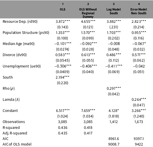
Replication of core results in Baller et al. (for 1990 only).

Standard errors in parentheses, ***
 $p<0.01$
, **
 $p<0.05$
, *
 $p<0.1$
.
To illustrate step 2 in the framework, we return to Baller et al.’s homicide study. The significance of the dummy variable for the South in Table 1 hints at the presence of spatial effects. Baller et al. specify spatial weights on the basis of the distance-related “nearest neighbor criterion,” using both 5 and 10 nearest neighbors (Baller et al.
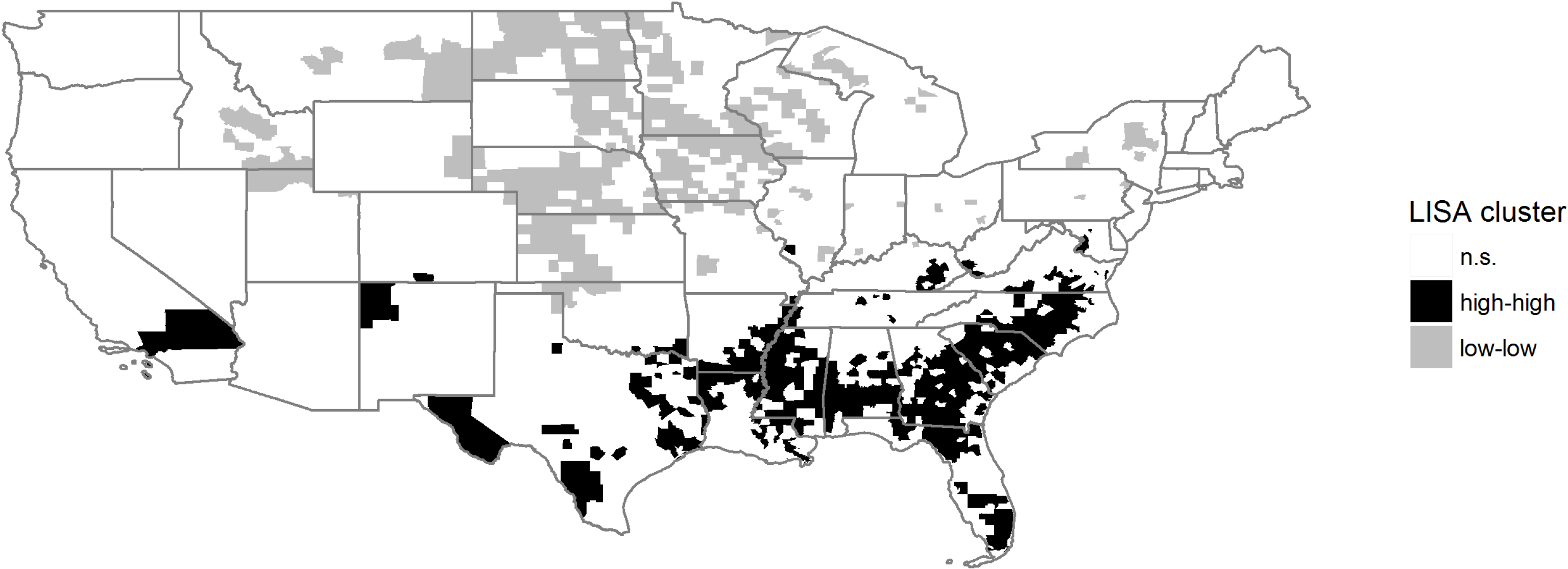
Reference Baller, Anselin, Messner, Deane and Hawkins2001, 572). In their data, the Global Moran’s I for 1990 is 0.37 and statistically significant at the .001 level. To visualize the spatial pattern of homicide rates, Figure 2 replicates the LISA cluster map reported as “Map 4” in Baller et al. (Reference Baller, Anselin, Messner, Deane and Hawkins2001, 577).Footnote
13
LISA stands for “local indicator of spatial autocorrelation” (Anselin Reference Anselin1995) and provides information on the correlation of an outcome of interest among a focal unit
 $i$
and the units to which
 $i$
is connected,
 $j$
(e.g.,
 $i$
’s neighbors,
 $j$
). It also indicates whether the association is positive (i.e., similar values) or negative (i.e., dissimilar values), and whether it is statistically significant. LISA statistics thus serve to identify local clusters. While the Global Moran’s I may suggest little spatial autocorrelation in the data overall, LISA values can identify smaller geographic areas where positive or negative clustering occurs.Footnote
14
In this case, the map shows clusters of high homicide rates across the South (black) and clusters of low homicide rates in the Upper Midwest and Northeast (gray). The overall higher incidence and spatial association of homicide in the South—clearly apparent in the map—is one of the reasons why scholars generally include a dummy for this region. The different clustering patterns across different parts of the U.S. also suggest two different spatial processes in the data.
LISA cluster map.

Once spatial dependence has been detected, the next step in the analysis depends on the nature of this dependence. More specifically, the question is which type of spatial dependence—spatial lag or error—best fits the data according to LM diagnostics. Although conceptually distinct, both processes may be happening at the same time. In such cases, LM diagnostics indicate which is more prominent. To determine the appropriate modeling strategy, researchers must assume that the same data-generating process is at work throughout the territory under study, and thus that coefficients are stable.
Returning to our homicide example, close inspection of the initial OLS diagnostics and the LISA map in Figure 2 lead Baller et al. (Reference Baller, Anselin, Messner, Deane and Hawkins2001) to question their assumption of coefficient stability and to suspect spatial heterogeneity between the South and non-South. Diagnostics indeed revealed that no one spatial regime fits the sample as a whole. They therefore decided to pursue a disaggregated modeling strategy and to estimate separate models for the South and non-South. LM diagnostics indicated that homicide follows a spatial lag structure in the South and a spatial error structure in the non-South.Footnote 15 Stated differently, Baller et al. find that once the variation in violence explained by other predictors of interest is considered, the remaining variation in homicide in any one unit in the South is best explained by the homicide rate in surrounding locations, suggesting the diffusion of violence from nearby communities and the need to identify vectors of transmission. Conversely, the remaining variation in homicide in any one location in the non-South is best explained by the remaining, unexplained component in nearby units, suggesting the need to identify previously unexamined or omitted variables.
The different spatial regimes in the two regions of the U.S. investigated by Baller et al. allow us to illustrate both the spatial lag and spatial error pathways in Figure 1, with each type of spatial dependence raising specific questions for the SNA. If a lag process is detected, the SNA provides the opportunity to uncover the mechanisms of diffusion—that is, what Baller et al. refer to as “vectors of transmission.” If dependence comes in the form of a spatial error process, the SNA can be leveraged to identify spatially clustered omitted variables. For both, insights from a geographically weighted regression (GWR) provide leverage for case selection. More specifically, GWR (Brunsdon, Fotheringham, and Charlton Reference Brunsdon, Fotheringham and Charlton1996; Fotheringham, Brunsdon, and Charlton Reference Fotheringham, Brunsdon and Charlton2002; Charlton, Fotheringham, and Brunsdon Reference Charlton and Fotheringham2009) enables exploring spatial heterogeneity in the data and investigating whether the magnitude, direction, or significance of predictors and the spatially lagged dependent variable is uneven across units. Formally, the baseline model would be adjusted as follows, so that a coefficient
 $\unicode[STIX]{x1D6FD}$
is estimated at each location
 $i$
, contrasting with the single coefficient estimated in the baseline model:
 $$\begin{eqnarray}y_{i}=\mathop{\sum }_{k}x_{ki}\unicode[STIX]{x1D6FD}_{ki}+\unicode[STIX]{x1D700}_{i}.\end{eqnarray}$$
In contrast to OLS or even conventional spatial regressions that assume a single, uniform relationship holds across all units, GWR allows “different relationships to exist at different points in space” (Brunsdon et al. Reference Brunsdon, Fotheringham and Charlton1996, 281), thereby facilitating the analysis of spatial heterogeneity (Shoff, Yi-Ju Chen, and Yang Reference Shoff, Yi-Ju Chen and Yang2014, 558). More specifically, GWR models estimate local coefficients and standard errors for each predictor of interest, generating information about the local statistical significance and substantive magnitude and direction of these predictors. To be clear, where Baller et al. were examining a discrete form of spatial heterogeneity by dividing the U.S. into two discrete spatial regimes, GWR examines a continuous form of spatial heterogeneity, allowing coefficients to vary not just across preidentified regions (South and non-South) but across all individual units (on discrete spatial heterogeneity, see Anselin and Rey Reference Anselin and Rey2014, chaps. 12, 13).
3.3 Step 3a: Conduct SNA to identify vectors of transmission for the spatial lag
In geo-nested analysis, insights gleaned at each stage of analysis set the agenda for the following stage. In situations where the spatial dependence in the data follows a spatial lag process, the SNA, we argue, may provide guidance for identifying vectors of transmission. In the homicide analysis, Baller et al. (Reference Baller, Anselin, Messner, Deane and Hawkins2001, 538) note that—despite statistical evidence for diffusion in the South—advancing a definitive argument “will require the identification and measurement of the precise mechanisms involved.” The SNA provides analytic leverage to pin down these mechanisms—that is, to identify how what happens in nearby places influences what happens locally, either simultaneously or sequentially over time.
Note that vectors of transmission are distinct from the spatial weights specified in the connectivity matrix. Spatial weights define other units with which any given unit is expected to interact, but say nothing about a causal process. Uncovering a vector of transmission therefore goes further than specifying a spatial weight. To identify a vector of transmission, we have to answer two questions: (1) in which other units will the outcome from the focal unit also appear; and (2) how and why is the appearance in both the focal unit and other units connected? Vectors of transmission are thus similar to causal mechanisms. While a causal mechanism in a nonspatial analysis specifies how
 $X$
caused
 $Y$
within the same unit (e.g., Falleti and Lynch Reference Falleti and Lynch2009), a vector of transmission indicates how an outcome in one place influenced an outcome elsewhere. The purpose of case selection for the SNA is thus to identify units in which we are most likely to uncover these vectors.
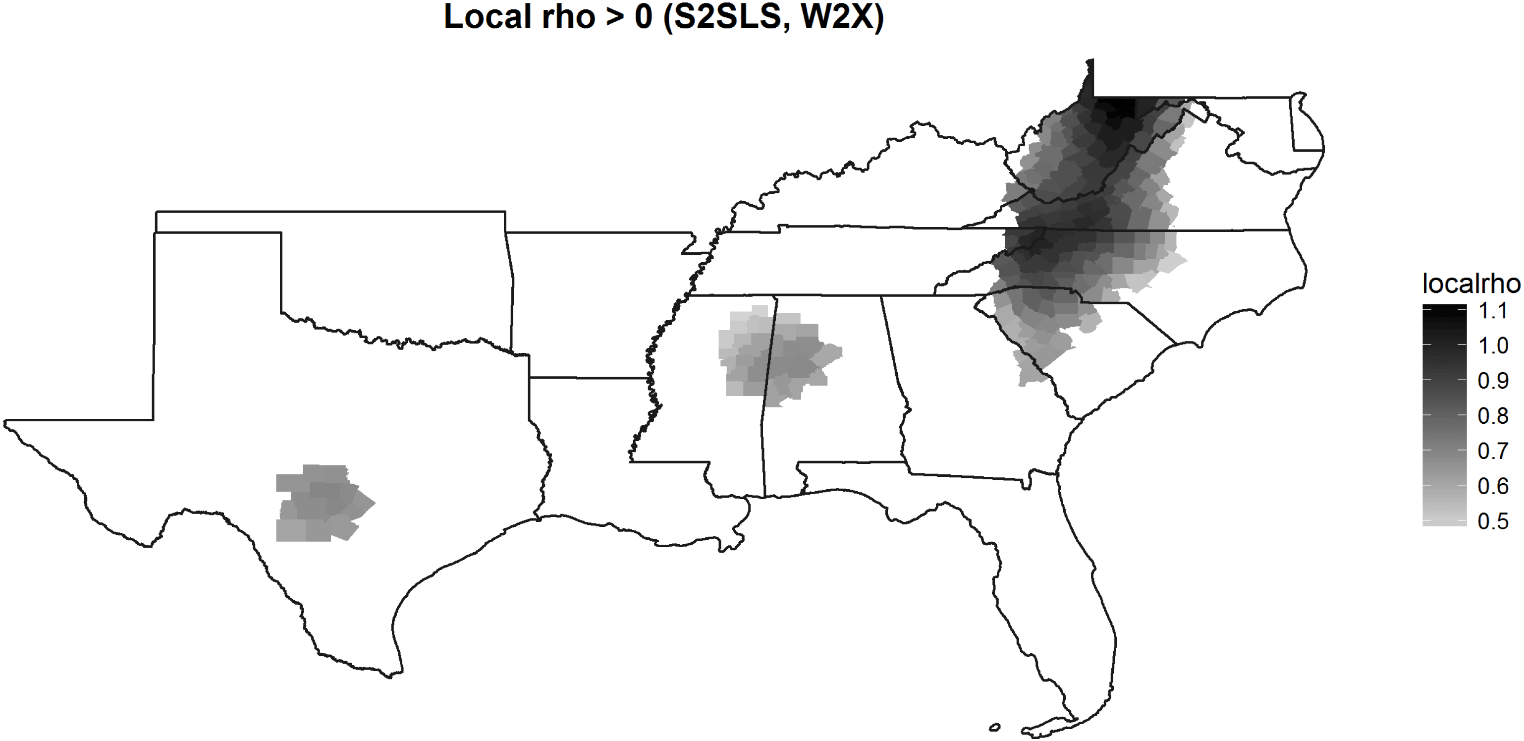
Map of local rho (positive values).

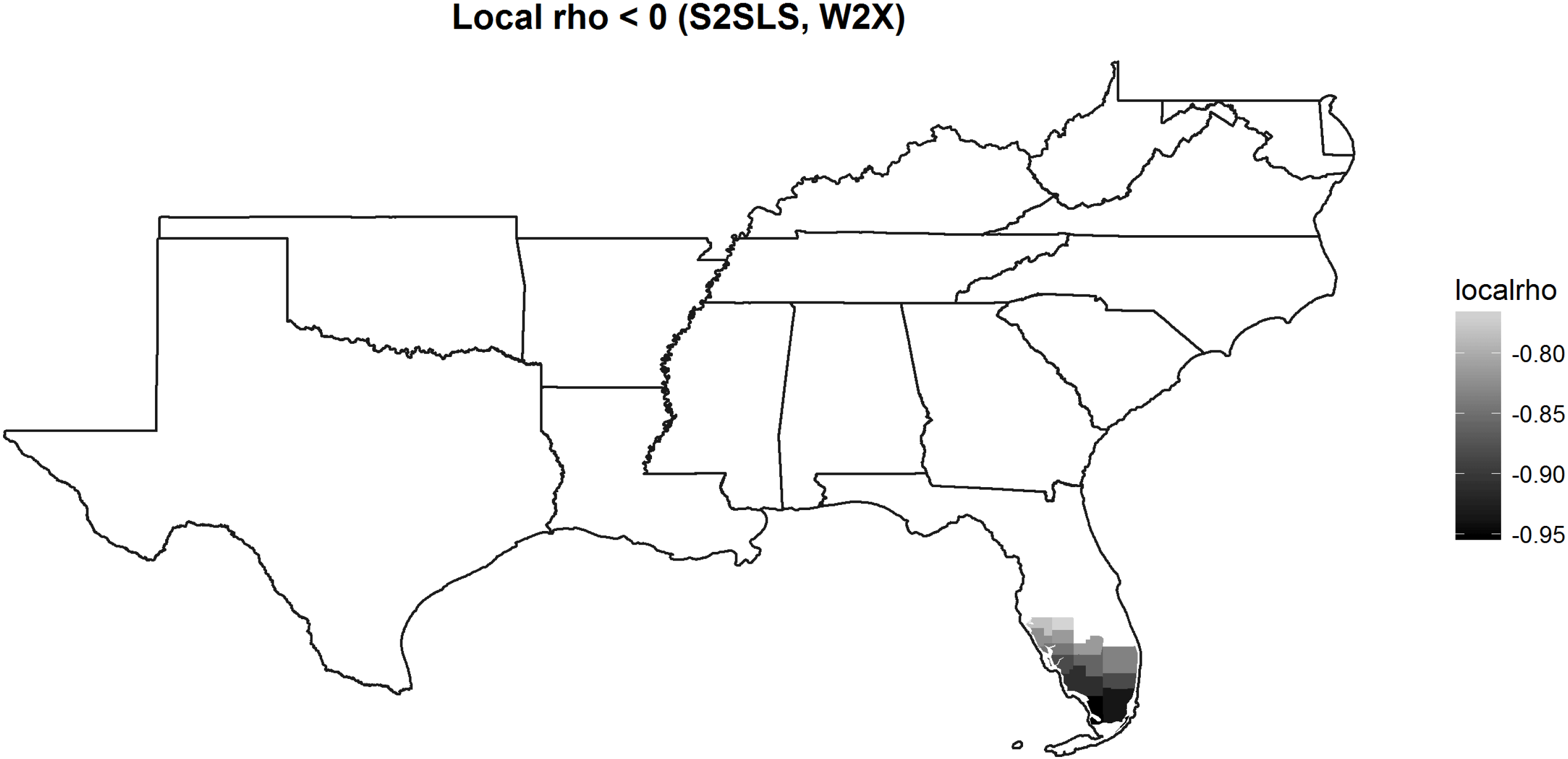
Map of local rho (negative values).

GWR provides a powerful tool to select these cases. By calculating the spatial lag of the outcome of interest and including this term as one of the predictors, we can specify a GWR-spatial lag model (GWR-SL; see Páez, Uchida, and Miyamoto Reference Páez, Uchida and Miyamoto2002; Shoff et al.
Reference Shoff, Yi-Ju Chen and Yang2014) and generate local estimates for the spatial lag term (
 $\unicode[STIX]{x1D70C}$
, rho). That is, we can estimate the locally varying effect of diffusion. Returning to our example, we specify the following model, where the spatial lag term (
 $Wy$
) is first estimated using the first-order and second-order lags of the explanatory variables as instruments (Anselin and Rey, 160–161; Kelejian and Prucha Reference Kelejian and Prucha2010, esp. fn 13):
 $$\begin{eqnarray}y_{i}=\sum \unicode[STIX]{x1D70C}_{i}W_{i}y+\mathop{\sum }_{k}x_{ki}\unicode[STIX]{x1D6FD}_{ki}+\unicode[STIX]{x1D700}_{i}.\end{eqnarray}$$
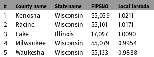
Figures 3 and 4 map the local coefficients for the spatial lag term (rho) in a GWR-SL model of the data in Table 1 but only for the 1,412 southern counties in the U.S. where Baller et al. find a spatial lag process (Model 3 in Table 1).Footnote 16 Whereas the results in Table 1 show a single, uniform, positive coefficient for the diffusion parameter (rho) in a standard spatial lag model (0.297 in Model 3), the maps in Figures 3 and 4 illustrate the locally varying intensity or magnitude, statistical significance, and direction of diffusion in a geographically weighted model of the same process. Figure 3 shows that rho has a statistically significant and positive effect across large portions of the southern region of the U.S. This relationship is particularly strong in a large set of dark gray counties straddling several states, including the western parts of Virginia, North Carolina, and South Carolina, almost all of West Virginia, and the eastern parts of Kentucky and Tennessee. Interestingly, in Figure 4, a set of counties in southern Florida exhibits a negative rho coefficient, suggesting obstacles to diffusion. In a substantial number of blank counties (i.e., white), homicide in nearby counties does not have a statistically significant relationship with homicide in a focal county.
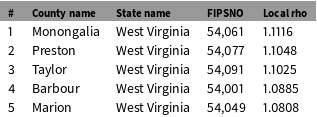
How can insights from the GWR-SL model guide case selection? And, following Lieberman, should case selection be deliberate or random? The answer to the second question depends on the outcome of the GWR, and whether or not meaningful variation in the spatial lag process can be identified. If the GWR suggests very little or no variation in rho throughout the sample, cases may be selected from the sample randomly, as each focal unit and its neighbors provide opportunities to examine the spatial process. But if the GWR reveals variation in the intensity of the spatial lag, as in Figures 3 and 4, case selection should be deliberate. In these instances, variation in rho can be leveraged to identify promising cases for identifying vectors of transmission. More specifically, a researcher may want to analyze cases with high rho values to uncover how the outcome of interest in a focal unit interacts with the outcome of interest in neighboring units. Notably, all five of the top values are counties in the state of West Virginia, marked by the darkest colors in Figure 3. Returning to our example, Table 2 identifies the five counties with the highest rho values—good candidates to serve as focal units for the SNA. Rho values can be positive, where an outcome in one unit increases the likelihood of similar outcomes in neighboring units, or negative, where an outcome decreases the likelihood of a similar outcome nearby. If rho is negative, as in Figure 4, the findings suggest barriers to diffusion or, even more provocatively, negative feedback effects (see “barrier counties” in Messner et al. Reference Messner, Anselin, Baller, Hawkins, Deane and Tolnay1999; also “diffusion proofing” in Koesel and Bunce Reference Koesel and Bunce2013). The identified counties in southern Florida, then, would be promising locations in which to explore the sources of this phenomenon.
In addition to selecting focal units with large positive or negative rho values, another promising case selection strategy is to analyze cases with significant rho values alongside those with nonsignificant rho values where both diffusion and negative feedback are presumably absent. The researcher would then be well placed to detect vectors of transmission among units with significant rho values and barriers to transmission in those where rho is not significant. Awareness of patterns in rho is valuable as it increases the likelihood of fruitful analysis during the SNA phase. Without knowledge of variation in rho, a researcher analyzing homicide diffusion might have chosen counties colored white in Figures 3 and 4 only to be disappointed by the results of the SNA.
Top 5 largest local rho coefficients.

Questions about substantive spatial dependence have generally remained outside the scope of systematic mixed-methods designs. To illustrate the added value of the SNA in a study of substantive spatial dependence—and the types of questions the SNA may address in the research process—we draw on another example of research on violence in the US South. Tolnay et al. (Reference Tolnay, Deane and Beck1996) conduct a quantitative analysis of spatial effects in the incidence of lynchings between 1890 and 1919. They argue that lynchings were a form of political violence—part of a state-tolerated repressive strategy to terrorize African–Americans and to preserve white supremacy. The authors find evidence for substantive spatial dependence as the likelihood of lynchings in a county is negatively associated with mob violence nearby. They hypothesize that this pattern can be explained by a “deterrence effect” as “whites were satisfied that local blacks were sufficiently threatened by nearby lynchings” and “blacks altered their behavior to minimize conflict with local whites” (788). A prerequisite for both mechanisms is that news about violent events spreads beyond the counties where they occurred. Tolnay et al. expect proximity to be associated with “more efficient transmission of information about lynchings” (792). In their quantitative analysis, geographic distance serves as proxy for channels of communication that cannot (yet) be adequately measured. To pin down a vector of transmission, an SNA would then aim to uncover whether and how news about violent incidents spreads from a focal unit to nearby counties. One possibility is that news about violence traveled primarily by word of mouth, in which case travel time or road networks may better capture the vector of transmission than Euclidean distance. Alternatively, lynchings may have been publicized in local newspapers, so that newspaper circulation or common membership in a regional media market may better capture the mechanisms underlying the spatial process.
The identification of vectors of transmission during the SNA entails a shift from dataset to causal-process observations (Collier et al. Reference Collier, Brady, Seawright, Brady and Collier2004). The appropriate technique for process tracing depends on the research question at hand (Bennett and Checkel Reference Bennett and Checkel2015). To probe the plausibility of the “deterrence effect” hypothesized by Tolnay et al., researchers would most likely rely on archival research—evidence of how news about lynchings spread, as well as how this was received by populations in surrounding counties. More contemporary research questions can make use of qualitative techniques including interviews, focus groups, and participatory observation. Qualitative work can take place at a distance (e.g., examining secondary literature or journalistic accounts online) or can be fieldwork consisting of personal interviews, observation, and visits to local archives. Crucially, the SNA focuses on linkages and interactions between units to better understand the spatial pattern.
In studies of substantive spatial dependence, the contribution of the SNA to the overall analysis is twofold. First, the SNA probes the plausibility of the causal claim underlying the LNA by identifying how an outcome in one place influenced events elsewhere. Second, the SNA can inform future iterations of the LNA by refining the specification of the connectivity matrix. Without a thorough understanding of the relationship between units, researchers often begin their analysis with a weights matrix specified on the basis of geographic space. This may ultimately turn out to be a placeholder for other forms of connectedness to be uncovered during the SNA phase. As noted earlier, researchers working in the reverse order—from SNA to LNA—would be advised to pay special attention to identifying vectors of transmission and optimal specifications of the connectivity matrix during the qualitative phase of work in order to develop better models during the large-N phase.
3.4 Step 3b: Conduct SNA to identify spatially clustered omitted variables
While a spatial lag process reflects a substantive relationship between units, a spatial error process suggests the presence of spatially clustered omitted variables. These variables may jeopardize inference if their presence is not modeled adequately, even though the spatial process is generally not of substantive interest. Variation in the error term, identified through GWR, provides leverage for informed case selection. More specifically, by calculating the spatial lag of the residuals and including this term as one of the predictors in a GWR model, we can specify a GWR-spatial error model (GWR-SE). The GWR-SE model generates local estimates for the spatial error term (
 $\unicode[STIX]{x1D706}$
, or lambda) and estimates the locally varying effect of unexplained, contextual factors. Returning to the homicide example, we specify the following model:
 $$\begin{eqnarray}y_{i}=\sum \unicode[STIX]{x1D706}_{i}W_{i}u+\mathop{\sum }_{k}x_{ki}\unicode[STIX]{x1D6FD}_{ki}+\unicode[STIX]{x1D700}_{i}.\end{eqnarray}$$
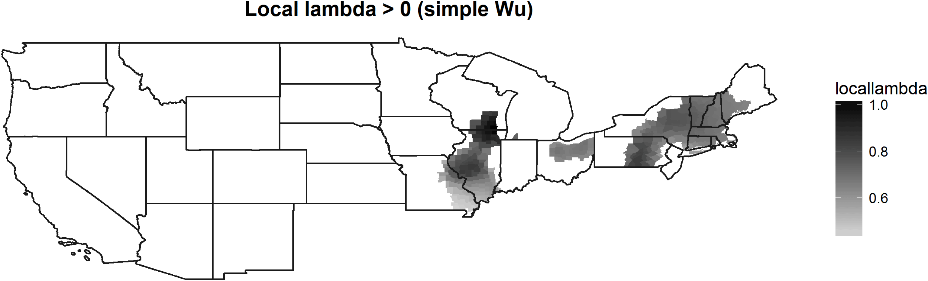
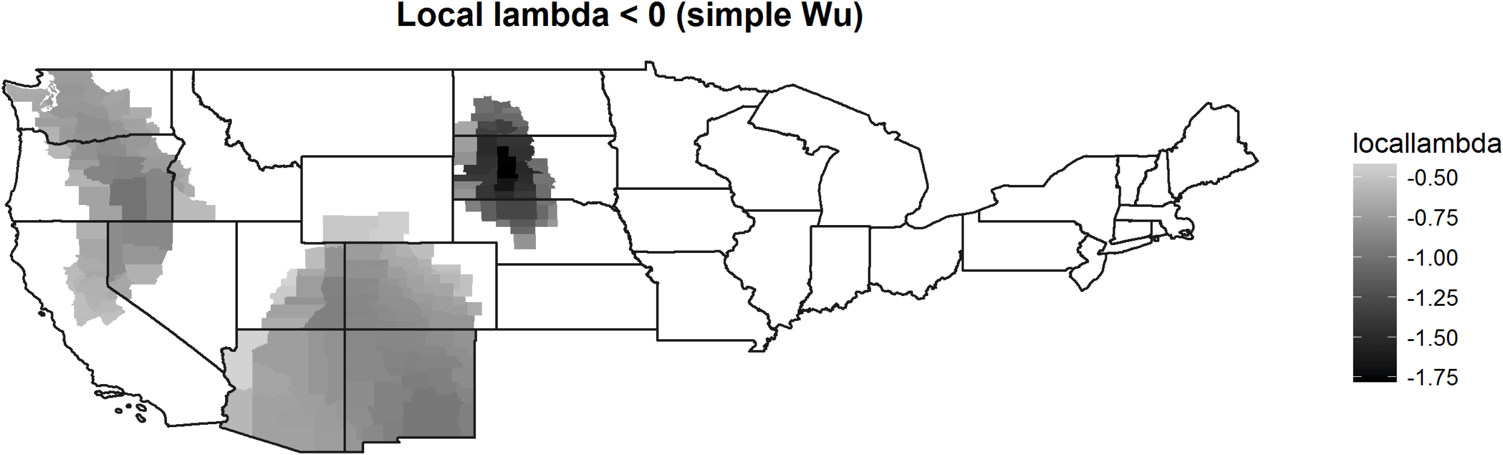
Figures 5 and 6 map the local coefficients for lambda in the 1,673 nonsouthern counties and show where lambda is significant and whether it is positive or negative.Footnote 17 In theory, it is possible that the GWR-SE model might not find variation. However, this is unlikely if the omitted variable is different across space, or if the effect of the omitted variable is uneven, i.e., the effect of the unobserved variable is itself nonstationary.
Map of local lambda (positive).

Map of local lambda (negative).

Based on the calculation and visualization of local lambdas, a researcher may pursue two distinct case selection strategies. The first is analogous to Lieberman’s Model-testing SNA; the second is in line with a Model-building SNA. The first strategy is particularly useful if the researcher is not interested in spatial relationships, but in the causal mechanisms underlying the theoretical variables already in the model. To conduct a Model-testing SNA, a researcher may then want to select cases from among the observations where lambda is not significant. In this group, following Lieberman, cases “on the line” with low residuals in the spatial error model are good candidates. Because lambda is not significant, the researcher might expect that—despite the presence of spatial dependence in the sample—the units selected for SNA are unaffected by the spatial process. Note that these units can be examined individually, without considering the relationship with their neighbors.
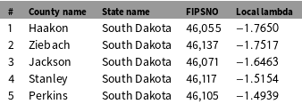
Second, researchers may want to uncover the omitted variables underlying the spatial process to generate new hypotheses, improve the model, and build theory. This is akin to a Model-building SNA. A promising case selection strategy would then be to select focal units with large (positive or negative) and significant values for lambda, and examine them along with their neighbors. This facilitates the identification of omitted variables that are causally linked to the dependent variable and present in similar forms or at similar levels in nearby units. While positive values for lambda suggest the presence of unmeasured covariates that increase the score on the dependent variable, in this case homicide rate, negative lambda values suggest the presence of factors that decrease the score. Illustrating this on the basis of our example, Tables 3 and 4 report the five largest and significant values for lambda for the sample, and the five lowest and significant values of lambda, respectively.
The identification of previously omitted variables has the potential to generate new hypotheses and thus to contribute to theory building. Once identified, these factors can be included in an expanded quantitative model (see Figure 1). During this next iteration of the LNA phase, LM diagnostics may no longer be able to detect spatial dependence. That is, the inclusion of previously omitted, spatially clustered variables may erase contextual effects previously captured by the spatial error term. Spatial dependence may thus disappear once new variables are added. To emphasize this last point, researchers interested in spatial processes may ultimately find that, at least for some portion of their phenomenon of interest, space does not matter. In other words, space was serving as a catch-all variable for mechanisms that were not fully modeled initially.
Five largest and significant values of local lambda.

Five smallest and significant values of local lambda.

4 Conclusion
In this paper, we have outlined case selection techniques for what we label “geo-nested analysis”—where case selection for SNA is based on diagnostics of a previously executed spatial-econometric analysis. We emphasize our commitment to an iterative research process, acknowledging that earlier stages of research generally inform later stages, but that later stages can also help evaluate earlier stages, leading researchers to revisit earlier analytic decisions.
With this iterative process in mind, Figure 1 offers a step-by-step overview for conducting geo-nested analysis. The first step is an OLS analysis containing only theoretically relevant variables. The second step is to check whether there is spatial dependence in the data and, if so, whether it follows a spatial lag or a spatial error process. If there is evidence for spatial lag, the SNA can be leveraged to identify vectors of transmission—that is, the causal mechanisms underlying diffusion. If there is evidence for spatial error, the purpose of the SNA is to uncover spatially clustered omitted variables, generate new hypotheses, and build theory. To be clear, both types of processes may be present in the data; while LM diagnostics help guide researchers about which process is most prominent, researchers need to remain aware of settings in which both processes are present. Still, in both scenarios, insights from GWRs can be used to select promising cases for in-depth analysis. With a GWR-spatial lag model (GWR-SL), we can detect clusters where the diffusion process is particularly pronounced, thus facilitating the identification of vectors of transmission. With a GWR-spatial error model (GWR-SE), we can identify clusters of local contextual factors not yet included in the model. In both scenarios, units should be examined along with their neighbors to better understand the origins and substantive meaning of spatial dependence. In sum, we advocate a mixed-methods strategy that emphasizes the need to examine sets of interdependent units, rather than individual units in isolation.
Funding
Imke Harbers gratefully acknowledges the financial support of an ERC Advanced Grant (Grant # 323899) and a Marie Curie Fellowship (Grant # 656361). Matthew Ingram acknowledges support from the Department of Political Science, the Rockefeller College of Public Affairs and Policy, and a Junior Researcher Award from the Center for Social and Demographic Analysis (CSDA) at the University at Albany, SUNY.