1. Introduction
Self-similarity has played an important role in shaping our understanding of fluid flows, particularly turbulence theory. Several problems in turbulence have been approached by self-preservation or self-similarity hypotheses imposing restrictions on the dynamics of the time dependence of the spectral functions (Monin, Yaglom & Lumley Reference Monin, Yaglom and Lumley1975). The first self-preservation hypothesis of isotropic turbulence was put forward by Von Kármán & Howarth (Reference Von Kármán and Howarth1938), in which the correlation functions or the equivalent spectral functions are reduced to functions of a single variable through an appropriate choice of a length scale
 $l(t)$
. The Von Kármán–Howarth equation
 $$\begin{eqnarray}\frac{\partial E(k,t)}{\partial t}=-2{\it\nu}k^{2}E(k,t)+T(k,t)\end{eqnarray}$$
describes the energy budget in spectral space for isotropic turbulence, where
 $k$
is the wavenumber,
 ${\it\nu}$
is the kinematic viscosity,
 $E(k,t)$
is the energy spectrum function and
 $T(k,t)$
is the spectral transfer function. Von Kármán’s hypotheses can be written in the form
 $$\begin{eqnarray}\displaystyle \left.\begin{array}{@{}c@{}}E(k,t)=l(t)s(t)^{2}f(kl),\\ T(k,t)=s(t)^{3}g(kl),\end{array}\right\} & & \displaystyle\end{eqnarray}$$
where the function
 $s(t)^{2}=\overline{u(t)^{2}}$
and
 $l(t)$
is a characteristic length scale.
Owing to the many simplifications to the governing equations, numerous previous investigations have focused on studying decaying temperature fluctuations in isotropic turbulence. For example, Warhaft & Lumley (Reference Warhaft and Lumley1978) showed that the decay of temperature fluctuations is greatly affected by initial conditions such as mean velocity, temperature and grid size.
The analysis of self-preservation, as conducted by Speziale & Bernard (Reference Speziale and Bernard1992) and George (Reference George1992a
), offered new approaches to the problem. George (Reference George1992a
) analysed the spectral energy equation (1.1) and concluded that it admits self-preservation solutions with the energy
 $\overline{q^{2}}$
decaying as
 $t^{-m}$
where
 $m$
depends on initial conditions. Speziale & Bernard (Reference Speziale and Bernard1992) considered the transport equation for two-point velocity correlations and the viscous rate of dissipation, and found two similarity solutions, with
 $\overline{q^{2}}\sim t^{-m}$
in the limit of vanishing Reynolds number and
 $\overline{q^{2}}\sim t^{-1}$
at high Reynolds number, which holds in the case where Reynolds number (
 $\mathit{Re}_{{\it\lambda}}$
) is constant. However, recent data at very high Reynolds number seem to contradict these predictions (Sinhuber, Bodenschatz & Bewley Reference Sinhuber, Bodenschatz and Bewley2015). George & Gibson (Reference George and Gibson1992) similarly investigated self-preservation of homogeneous shear flow turbulence and identified the velocity scale as the turbulent kinetic energy
 $q^{2}$
and the characteristic length scale as the Taylor microscale
 ${\it\lambda}$
. The authors identified two cases of self-preserving flows, a constant mean shear and a mean shear that is inversely proportional to time. For a constant mean shear the turbulence grew exponentially in time. In addition, the authors showed that the spectral shape strongly depends on initial conditions.
In the case of passive scalars, George (Reference George, Gatski, Speziale and Sarkar1992b
) considered the spectral equations governing the decay of temperature fluctuations in isotropic turbulence, and found that the characteristic length scale is the scalar Taylor microscale and that the scaling function is the scalar variance. This analysis agrees reasonably well with the energy spectra of Comte-Bellot & Corrsin (Reference Comte-Bellot and Corrsin1971) and the temperature spectra of Warhaft & Lumley (Reference Warhaft and Lumley1978), especially at higher wavenumbers. Benaissa et al. (Reference Benaissa, Djenidi, Antonia and Parker2007) considered decaying grid turbulence at low Reynolds number (
 $\mathit{Re}_{{\it\lambda}}\sim 50$
) for different initial conditions, where heat was injected using a mandoline, and showed that the decay depends on the initial conditions. In addition, the authors showed that the second-order temperature structure functions collapse when normalized with the temperature variance and the scalar Taylor microscale. A similarity analysis was performed by Antonia et al. (Reference Antonia, Smalley, Zhou, Anselmet and Danaila2004) and applied to data from a grid and heated mandoline combination, to show that the second-order structure function satisfies similarity and collapses with the temperature variance and the Taylor microscale.
In this work, self-preservation of the temperature spectral equations is investigated for grid turbulence with the addition of a mean cross-stream temperature gradient. In this particular configuration, turbulence is decaying while temperature variance is generated by interaction with the mean temperature gradient and dissipated through the action of thermal diffusivity. This flow has been widely investigated in previous studies, for example in the work of Warhaft (Reference Warhaft2000); however, it has not been approached from a self-preservation perspective. In this configuration, the temperature field is passive and governed by the equation
 $$\begin{eqnarray}\frac{1}{2}\frac{\text{d}\overline{{\it\theta}^{2}}}{\text{d}t}=-\overline{{\it\theta}v}{\it\beta}-{\it\epsilon}_{{\it\theta}},\end{eqnarray}$$
where
 $\overline{{\it\theta}^{2}}$
is the temperature variance, with
 ${\it\theta}$
being the instantaneous temperature,
 ${\it\beta}$
is a constant mean temperature gradient,
 $v$
is the instantaneous cross-stream velocity fluctuation and
 ${\it\epsilon}_{{\it\theta}}$
is the scalar rate of dissipation. It can be seen that the rate of change of temperature variance is affected by production and dissipation. The scalar rate of dissipation is defined by
 $$\begin{eqnarray}{\it\epsilon}_{{\it\theta}}={\it\alpha}\overline{\frac{\partial {\it\theta}}{\partial x_{i}}\frac{\partial {\it\theta}}{\partial x_{i}}}.\end{eqnarray}$$
In this study, we are particularly interested in the spectral equation governing this flow, i.e.
 $$\begin{eqnarray}\frac{\partial E_{{\it\theta}}}{\partial t}=-{\it\beta}E_{v{\it\theta}}-2{\it\alpha}k^{2}E_{{\it\theta}}+T_{{\it\theta}},\end{eqnarray}$$
where
 $E_{{\it\theta}}$
is the spectrum of scalar variance,
 $E_{v{\it\theta}}$
is the spectrum of scalar flux and
 $T_{{\it\theta}}$
is the spectral transfer function.
It will be shown that, for the case of the temperature variance spectra, similar to (1.2),
 $E_{{\it\theta}}(k,t)=\ell _{{\it\theta}}(t)s_{{\it\theta}}(t)^{2}f_{{\it\theta}}(k\ell _{{\it\theta}})$
, where
 $s_{{\it\theta}}(t)^{2}$
can be regarded as
 $\overline{{\it\theta}(t)^{2}}$
. For self-preserving solutions to exist, a characteristic length scale
 $\ell _{{\it\theta}}(t)$
must be defined. According to Kolmogorov’s hypotheses, the small-scale turbulence is characterized by the kinematic viscosity and the rate of dissipation. Therefore, if expressed in Kolmogorov variables, the probability distributions of small-scale velocity fluctuations for different Reynolds numbers are identical. For temperature fluctuations, the common approach is to consider Corrsin (Reference Corrsin1964) or Batchelor (Reference Batchelor1959) scales, each of which applies for different ranges of Prandtl number
 $\mathit{Pr}={\it\nu}/{\it\alpha}$
. For fluids of Prandtl number close to unity, such as air considered in this work, these two scales are equivalent. For consistency, the Batchelor scale
 ${\it\eta}_{{\it\theta}}$
is adopted to represent these two scales throughout this work:
 $$\begin{eqnarray}{\it\eta}_{{\it\theta}}=\frac{{\it\eta}}{\sqrt{\mathit{Pr}}},\end{eqnarray}$$
where
 ${\it\eta}$
is the Kolmogorov microscale.
The remainder of the paper is as follows. The conditions for which self-preserving solutions exist are derived in § 2. A brief description of the experimental set-up is presented in § 3, and the experimental data are investigated for self-similarity in § 4.
2. Similarity analysis
The evolution of a passive scalar in grid turbulence with a mean cross-stream temperature gradient is investigated from a self-preservation perspective. In this particular study, the primary objective is to establish self-preserving solutions of (1.5), for which all terms remain in relative balance. As can be seen, in contrast to previous investigations, (1.5) includes an additional term (
 $-{\it\beta}E_{v{\it\theta}}$
), resulting from the production of temperature variance.
To seek self-similarity of (1.5), a solution of the form
 $$\begin{eqnarray}\displaystyle \left.\begin{array}{@{}c@{}}E_{{\it\theta}}=E_{s,{\it\theta}}(t)f_{1}({\it\gamma}),\\ T_{{\it\theta}}=T_{s,{\it\theta}}(t)g_{1}({\it\gamma}),\\ E_{v{\it\theta}}=E_{s,v{\it\theta}}(t)f_{2}({\it\gamma})\end{array}\right\} & & \displaystyle\end{eqnarray}$$
is assumed. In the equations,
 ${\it\gamma}=k\ell _{i}$
is the similarity variable, where
 $\ell _{i}$
is a characteristic length scale of the flow (
 $\ell _{v}$
for the energy spectra equation,
 $\ell _{{\it\theta}}$
for the temperature equation and
 $\ell _{v{\it\theta}}$
for the temperature flux equation), and
 $E_{s,{\it\theta}}(t)$
,
 $T_{s,{\it\theta}}(t)$
and
 $E_{s,v{\it\theta}}(t)$
are the respective scaling functions. By assuming the above solution, (1.5) reads
 $$\begin{eqnarray}[{\dot{E}}_{s,{\it\theta}}]\,f_{1}+\left[E_{s,{\it\theta}}\frac{\dot{\ell }_{{\it\theta}}}{\ell _{{\it\theta}}}\right]f_{1}^{\prime }{\it\gamma}=-[{\it\beta}E_{s,v{\it\theta}}]\,f_{2}-[T_{s,{\it\theta}}]g_{1}-\left[{\it\alpha}\frac{E_{s,{\it\theta}}}{\ell _{{\it\theta}}^{2}}\right]2{\it\gamma}^{2}f_{1},\end{eqnarray}$$
where the prime denotes differentiation with respect to
 ${\it\gamma}$
and the dot is the time rate of change. For self-similarity to hold, the terms in brackets must have same time dependence. Consequently, a set of conditions can be found as
 $$\begin{eqnarray}\displaystyle & \displaystyle \left[{\dot{E}}_{s,{\it\theta}}\frac{\ell _{{\it\theta}}^{2}}{{\it\alpha}E_{s,{\it\theta}}}\right]={\it\epsilon}_{1}, & \displaystyle\end{eqnarray}$$
 $$\begin{eqnarray}\displaystyle & \displaystyle [{\it\alpha}\ell _{{\it\theta}}\dot{\ell }_{{\it\theta}}]={\it\epsilon}_{2}, & \displaystyle\end{eqnarray}$$
 $$\begin{eqnarray}\displaystyle & \displaystyle \left[{\it\beta}\frac{E_{s,v{\it\theta}}}{{\it\alpha}E_{s,{\it\theta}}}\ell _{{\it\theta}}^{2}\right]={\it\epsilon}_{3}, & \displaystyle\end{eqnarray}$$
 $$\begin{eqnarray}\displaystyle & \displaystyle \left[\frac{T_{s,{\it\theta}}}{{\it\alpha}E_{s,{\it\theta}}}\ell _{{\it\theta}}^{2}\right]={\it\epsilon}_{4}, & \displaystyle\end{eqnarray}$$
 ${\it\epsilon}_{1}$
,
 ${\it\epsilon}_{2}$
,
 ${\it\epsilon}_{3}$
and
 ${\it\epsilon}_{4}$
are constants. For the remainder of the analysis, the primary focus is on the conditions presented in (2.3)–(2.6), but a similar analysis can be performed for the scalar flux, which is governed by
 $$\begin{eqnarray}\frac{\partial E_{v{\it\theta}}}{\partial t}=-{\it\beta}E+({\it\nu}+{\it\alpha})k^{2}E_{v{\it\theta}}+T_{v{\it\theta}},\end{eqnarray}$$
from which the following set of similarity conditions is reached:
 $$\begin{eqnarray}\left[{\dot{E}}_{s,v{\it\theta}}\frac{\ell _{v{\it\theta}}^{2}}{({\it\alpha}+{\it\nu})E_{s,v{\it\theta}}}\right]\sim [({\it\alpha}+{\it\nu})\ell _{v{\it\theta}}\dot{\ell }_{v{\it\theta}}]\sim \left[{\it\beta}\frac{E_{s}}{{\it\alpha}E_{s,v{\it\theta}}}\ell _{v{\it\theta}}^{2}\right]\sim \left[\frac{T_{s,v{\it\theta}}}{({\it\alpha}+{\it\nu})E_{s,v{\it\theta}}}\ell _{v{\it\theta}}^{2}\right]\sim {\it\epsilon}_{v{\it\theta}},\end{eqnarray}$$
where
 ${\it\epsilon}_{v{\it\theta}}$
is a constant. Similarly, (1.1) dictates self-preserving solutions to the spectral equations associated with the velocity field as
 $$\begin{eqnarray}\left[{\dot{E}}_{s}\frac{\ell _{v}^{2}}{{\it\nu}E_{s}}\right]\sim [{\it\nu}\ell _{v}\dot{\ell }_{v}]\sim \left[\frac{T_{s}}{{\it\nu}E_{s}}l_{v}^{2}\right]\sim {\it\epsilon}_{v},\end{eqnarray}$$
where
 ${\it\epsilon}_{v}$
is a constant.
Next, the characteristic length scale
 $\ell _{{\it\theta}}$
is derived from the similarity conditions. Integrating (2.4) where the constant is
 ${\it\epsilon}_{2}={\it\alpha}A_{{\it\theta}}$
reveals the time dependence of
 $\ell _{{\it\theta}}$
to be
 $$\begin{eqnarray}\ell _{{\it\theta}}^{2}=\ell _{0{\it\theta}}^{2}+A_{{\it\theta}}(t-t_{0}),\end{eqnarray}$$
where
 $\ell _{0{\it\theta}}$
is a constant and
 $t_{0}$
is a virtual origin in time. The scaling function
 $E_{s,{\it\theta}}$
can be related to physical quantities, particularly
 $\ell _{{\it\theta}}$
and the temperature variance
 $\overline{{\it\theta}^{2}}$
, by considering the definition of the spectrum of the temperature variance,
 $$\begin{eqnarray}\overline{{\it\theta}^{2}}=\int _{0}^{\infty }E_{{\it\theta}}(k,t)\,\text{d}k=\left(\frac{E_{s,{\it\theta}}}{\ell _{{\it\theta}}}\right)\int _{0}^{\infty }f_{1}({\it\gamma})\,\text{d}{\it\gamma},\end{eqnarray}$$
from which we deduce, without loss of generality, that
 $$\begin{eqnarray}E_{s,{\it\theta}}=\overline{{\it\theta}^{2}}\ell _{{\it\theta}}.\end{eqnarray}$$
Knowing the form of
 $E_{s,{\it\theta}}$
(2.12) and given that (2.4) provides a solution for
 $\ell _{{\it\theta}}$
, the similarity conditions dictate the dynamics of the temperature variance
 $\overline{{\it\theta}^{2}}$
for the existence of a self-preserving solution. In particular, (2.3) provides a form of the scaling function
 $E_{s,{\it\theta}}$
, given that the characteristic scale follows (2.10),
 $$\begin{eqnarray}\ln E_{s,{\it\theta}}=C_{1}\frac{{\it\alpha}}{A_{{\it\theta}}}\ln (l_{0{\it\theta}}^{2}+A_{{\it\theta}}(t-t_{0}))+\ln C_{2}=C_{1}\frac{{\it\alpha}}{A_{{\it\theta}}}\ln \ell _{{\it\theta}}^{2}+\ln C_{2},\end{eqnarray}$$
where
 $C_{1}$
and
 $C_{2}$
are constants. Equation (2.13) implies a form for the temperature variance given by
 $$\begin{eqnarray}\overline{{\it\theta}^{2}}=C_{2}[\ell _{{\it\theta}}]^{(2C_{1}{\it\alpha}/A_{{\it\theta}})-1}.\end{eqnarray}$$
3. Experimental set-up
The experimental investigation is conducted in a grid turbulence set-up with an imposed mean cross-stream temperature gradient
 ${\it\beta}$
. The authors acquired temperature data in an open-loop wind tunnel with a 9.1 m (30 ft) long test section,
 $0.91~\text{m}\times 0.91~\text{m}$
(
 $3~\text{ft}\times 3~\text{ft}$
) cross-section, and a passive grid with mesh size
 $M=2.54~\text{cm}$
. The mean temperature gradient, generated by 32 heated coils placed in a parallel array upstream of the grid, maintains itself throughout the test section (Corrsin Reference Corrsin1952; Sirivat & Warhaft Reference Sirivat and Warhaft1983). The wind tunnel is located at Cornell University, and more details about the experimental set-up can be found in Yoon & Warhaft (Reference Yoon and Warhaft1990).
Data were acquired using a novel microelectromechanical system (MEMS) based temperature sensor, T-NSTAP, developed to minimize both temporal and spatial filtering on the data. The T-NSTAP was designed following the model described in Arwatz, Bahri & Smits (Reference Arwatz, Bahri, Smits and Hultmark2013), with a superior frequency response compared to conventional cold-wire probes. More details about the T-NSTAP, its performance and comparison to conventional cold wires can be found in Arwatz et al. (Reference Arwatz, Fan, Bahri and Hultmark2015).
The T-NSTAP was operated with a constant current of 0.05 mA. The temperature time signal was digitized at a sampling rate of 50 kHz for up to 600 s and low-pass-filtered at 25 kHz. Velocity data were acquired using a hot wire with
 $2.5~{\rm\mu}\text{m}$
diameter at a sampling rate of 300 kHz for 300 s using a 16 bit analogue-to-digital (A/D) converter and low-pass-filtered with a cut-off frequency of 150 kHz.
Various downstream positions (
 $x/M$
ranging between 8 and 200) for
 $M=2.54~\text{cm}$
were studied for two different initial conditions: (i) a mean streamwise velocity
 $U=6~\text{m}~\text{s}^{-1}$
and a mean temperature gradient
 ${\it\beta}=5~\text{K}~\text{m}^{-1}$
, corresponding to
 $\mathit{Re}_{M}=MU/{\it\nu}=9090$
(case I), and (ii) a mean velocity of
 $U=9~\text{m}~\text{s}^{-1}$
and a mean temperature gradient of
 ${\it\beta}=8~\text{K}~\text{m}^{-1}$
, corresponding to
 $\mathit{Re}_{M}=13\,630$
(case II). By using the same set-up, Sirivat & Warhaft (Reference Sirivat and Warhaft1983) and Jayesh, Tong & Warhaft (Reference Jayesh, Tong and Warhaft1994) showed that, for these conditions, temperature behaves as a passive scalar. The Reynolds number
 $\mathit{Re}_{L}$
, where
 $L$
is the integral length scale, ranged from 75 to 330 and 130 to 600 for
 $\mathit{Re}_{M}=9090$
and
 $\mathit{Re}_{M}=13\,630$
, respectively. The Taylor Reynolds number
 $\mathit{Re}_{{\it\lambda}}=u{\it\lambda}/{\it\nu}$
, where
 ${\it\lambda}$
is the Taylor microscale, varied from 35 to 100 and from 45 to 120 for
 $\mathit{Re}_{M}=9090$
and
 $\mathit{Re}_{M}=13\,630$
, respectively.
4. Results
Although thorough studies of this flow have been performed previously (Sirivat & Warhaft Reference Sirivat and Warhaft1983; Warhaft Reference Warhaft2000), this is the first time that self-similarity of the temperature field in grid turbulence with a constant mean temperature gradient has been investigated. In order to relate the similarity analysis described in § 2 to the one-dimensional measured temperature spectra, the following isotropic relation is used:
 $$\begin{eqnarray}E_{{\it\theta}}=-k\frac{\text{d}F_{{\it\theta}}}{\text{d}k},\end{eqnarray}$$
where
 $F_{{\it\theta}}$
is the measured one-dimensional temperature spectrum. It should be noted that, for the present flow, the large-scale thermal field is expected to be anisotropic while the assumption of small-scale isotropy is reasonable. Sirivat & Warhaft (Reference Sirivat and Warhaft1983) observed that the assumption of small-scale isotropy is still valid for this flow, by calculating the scalar rate of dissipation using three different methods, two of which assume isotropy. In other flow conditions, such as with the addition of a mean velocity gradient, the temperature derivative shows significant skewness; however, Sirivat & Warhaft (Reference Sirivat and Warhaft1983) showed that, in their experiments, the magnitude of the skewness of the temperature derivative is small (
 ${<}0.15$
). It has previously been observed that different parameters of the temperature field exhibit homogeneity for
 $x/M\gtrsim 40$
. By inspecting the cross-stream profiles of the standard deviation of temperature for grid turbulence with a linear mean temperature profile, Sirivat & Warhaft (Reference Sirivat and Warhaft1983) observed the establishment of a homogeneous profile by
 $x/M>40$
. A value of
 $x/M=30$
was found by Antonia et al. (Reference Antonia, Smalley, Zhou, Anselmet and Danaila2004) for a heated grid set-up. As shown by Arwatz et al. (Reference Arwatz, Fan, Bahri and Hultmark2015), the current data also suggest that a homogeneous flow is established beyond
 $x/M\sim 40$
. Subsequently, the existence of self-preserving solutions was investigated beyond this limit.
The similarity analysis presented above predicts the scaling function
 $E_{s,{\it\theta}}$
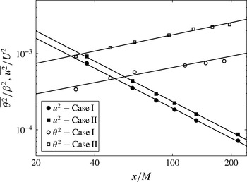
to be a function of the temperature variance. Figure 1 presents the evolution of velocity and temperature variance with streamwise location
 $x/M$
, on a logarithmic scale. As shown, temperature variance increases following a power law, owing to the imposed mean temperature gradient resulting in a non-zero production term in (1.3), while turbulence intensity decays as a power law, owing to the lack of production of turbulent kinetic energy. As indicated in the figure, the velocity variance for both initial conditions decays with the same power. In addition, a power-law behaviour, consistent with the similarity result presented in (2.14), is observed for the temperature variance, indicating a similar growth rate for both initial conditions. As the characteristic length scale (2.10) suggests the possibility of a non-zero virtual origin, the temperature and velocity variance data were used to estimate its location using the method outlined in Comte-Bellot & Corrsin (Reference Comte-Bellot and Corrsin1966), revealing that
 $x_{0}/M<1$
for both fields. Therefore, the virtual origin is dropped from the equations under consideration; however, the effect of a virtual origin is shown below.
Evolution of velocity and temperature variance with streamwise position
 $x/M$
. Solid lines represent power-law fits to the data:
 $\overline{u^{2}}\sim x^{-1.3}$
for both initial conditions,
 $\overline{{\it\theta}^{2}}\sim x^{0.51}$
for case II and
 $\overline{{\it\theta}^{2}}\sim x^{0.49}$
for case I.

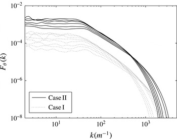
Figure 2 shows the unscaled spectra of temperature variance for different streamwise positions and two different initial conditions. In order to investigate the applicability of the similarity conditions to this particular flow, and specifically the validity of the scaling function
 $E_{s,{\it\theta}}$
in revealing self-preserving solutions, the spectra are scaled by the scaling function
 $E_{s,{\it\theta}}\sim \overline{{\it\theta}^{2}}x^{m}$
and the value of
 $m$
that best scales the data is explored. A new method to determine the quality of the scaling was developed. The coefficient of variation,
 ${\it\sigma}$
, of the scaled temperature spectra
 $E_{{\it\theta}}/E_{s,{\it\theta}}$
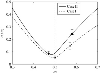
was inspected for different streamwise positions and averaged for all wavenumbers. Figure 3 presents
 ${\it\sigma}$
for different exponents,
 $m$
, normalized by the coefficient of variation
 ${\it\sigma}_{0}$
of the unscaled data. It can be seen that, according to the data, the coefficient of variation reaches a minimum at
 $m=0.495$
for case I and
 $m=0.49$
for case II.
One-dimensional measured temperature spectra for two different initial conditions, cases I and II, for streamwise positions
 $x/M$
ranging from 40 to 200.

Coefficient of variation
 ${\it\sigma}$
normalized by the coefficient of variation of the unscaled data
 ${\it\sigma}_{0}$
versus different exponents,
 $m$
, of the characteristic length scale in the scaling function
 $E_{s,{\it\theta}}$
, for two different initial conditions (cases I and II). The symbols correspond to different length scales: circles, Taylor microscale; triangles, Batchelor length scale. The vertical dashed line corresponds to the predicted similarity solutions, and error bars represent the effect of a virtual origin
 $x_{0}/M\pm 3$
.

The symbols shown in the figure relate to the coefficient of variation obtained by scaling the temperature spectra with the exponent,
 $m$
, that corresponds to the Taylor microscale and the Batchelor scale. The similarity analysis presented in § 2 suggests that, if self-preserving solutions exist, the characteristic length scale should follow the form given by (2.10). In particular, for a zero virtual origin, (2.10) implies a
 $t^{0.5}$
(or
 $x^{0.5}$
) dependence, marked by the vertical dashed line in figure 3. The data suggest that a similarity solution exists, and among the investigated length scales the Taylor microscale scales the spectra better and follows a power that is close to the power found by the similarity analysis.
This result can also be deduced by inspecting the scalar rate of dissipation and (2.12) as follows:
 $$\begin{eqnarray}{\it\epsilon}_{{\it\theta}}=2{\it\alpha}\int _{0}^{\infty }k^{2}E_{{\it\theta}}(k,t)\,\text{d}k=2\left[\frac{{\it\alpha}E_{s,{\it\theta}}}{\ell _{{\it\theta}}^{3}}\right]\int _{0}^{\infty }{\it\gamma}^{2}f_{1}({\it\gamma})\,\text{d}{\it\gamma}.\end{eqnarray}$$
From this it can be deduced that
 $$\begin{eqnarray}{\it\epsilon}_{{\it\theta}}\propto {\it\alpha}\frac{\overline{{\it\theta}^{2}}}{\ell _{{\it\theta}}^{2}}.\end{eqnarray}$$
In addition, considering the following relation of the scalar rate of dissipation to the scalar Taylor microscale
 ${\it\lambda}_{{\it\theta}}$
, specifically
 $$\begin{eqnarray}{\it\epsilon}_{{\it\theta}}=6{\it\alpha}\frac{\overline{{\it\theta}^{2}}}{{\it\lambda}_{{\it\theta}^{2}}},\end{eqnarray}$$
it can be deduced that
 $\ell _{{\it\theta}}\propto {\it\lambda}_{{\it\theta}}$
. Although the data indicate that the virtual origin is close to zero, it is particularly revealing to look at the effect of a virtual origin. The bars shown in figure 3 present the effect of a virtual origin of
 $x_{0}/M\pm 3$
on the coefficient of variation. As indicated, the existence of a small virtual origin does not greatly affect the scaling.
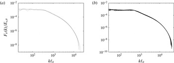
Figure 4(a,b) shows the one-dimensional spectra of figure 2 scaled by
 $\ell _{{\it\theta}}\sim (x/M)^{0.5}$
, as suggested by the similarity analysis, a value very close to the exponent corresponding to the minimum coefficient of variation and to the Taylor microscale. The uniformity of the collapse for different streamwise locations is remarkable and is good at most wavenumbers, particularly in the inertial and dissipation range. Some deviation from a uniform collapse at low wavenumbers is observed for spectra corresponding to locations closer to the grid, which might be due to initial conditions of the flow or to adjustment of the flow to the mean temperature gradient. However, overall, the collapse is convincing and supports the existence of a similarity solution.
One-dimensional measured temperature spectra scaled by
 $E_{s,{\it\theta}}=\overline{{\it\theta}^{2}}\ell _{{\it\theta}}$
, where
 $\ell _{{\it\theta}}\sim (x/M)^{m}$
with
 $m=0.5$
, for two different initial conditions (cases I and II) for streamwise positions
 $x/M$
ranging from 40 to 200.

An interesting consequence of a similarity solution can be observed by considering (2.11), and the definition of the scalar integral scale:
 $$\begin{eqnarray}L_{{\it\theta}}=\frac{{\rm\pi}}{2\overline{{\it\theta}^{2}}}\int _{0}^{\infty }\frac{E_{{\it\theta}}(k)}{k}\,\text{d}k.\end{eqnarray}$$
If the flow is governed by a similarity solution, as suggested above, the integral length scale should relate to the characteristic length scale as
 $$\begin{eqnarray}L_{{\it\theta}}\propto \ell _{{\it\theta}}\int _{0}^{\infty }\frac{f({\it\gamma})}{{\it\gamma}}\,\text{d}{\it\gamma}.\end{eqnarray}$$
Since
 $f$
is a function of
 ${\it\gamma}$
only,
 $L_{{\it\theta}}\propto \ell _{{\it\theta}}$
, and according to above observations
 $L_{{\it\theta}}\propto {\it\lambda}_{{\it\theta}}$
. In addition to the scaling of the spectra, this serves as another way to verify if the flow is self-similar. However, the current data do not support this criterion, and instead show
 ${\it\lambda}_{{\it\theta}}\propto x^{0.47}$
while
 $L_{{\it\theta}}\propto x^{0.34}$
. As the integral length scale measurements relate to the large scales in the wind tunnel, this discrepancy might be related to an experimental bias due to the finite-size wind tunnel or large and slow background fluctuations in the temperature field contaminating the integral length scale. It should be noted that both the velocity integral scale and the scalar integral scale measurement and evolution have been investigated by numerous previous studies (Comte-Bellot & Corrsin Reference Comte-Bellot and Corrsin1966; Sirivat & Warhaft Reference Sirivat and Warhaft1983; Overholt & Pope Reference Overholt and Pope1996; Fossen & Ching Reference Fossen and Ching1997; Wang & George Reference Wang and George2002; O’Neill et al.
Reference O’Neill, Nicolaides, Honnery and Soria2004; Donzis, Sreenivasan & Yeung Reference Donzis, Sreenivasan and Yeung2005), which points to the subtlety involved in those measurements. Looking at various investigations, Comte-Bellot & Corrsin (Reference Comte-Bellot and Corrsin1966) observed that different data indicate that the power-law exponent for the velocity integral scale growth varies between 0.34 and 0.53. For example, Sirivat & Warhaft (Reference Sirivat and Warhaft1983) studied the influence of varying the thermal scale relative to the velocity scale on the evolution of the flow and observed the evolution of the scalar integral scale to be proportional to
 $x^{0.35}$
. Other studies (Wang & George Reference Wang and George2002; O’Neill et al.
Reference O’Neill, Nicolaides, Honnery and Soria2004) assessed and observed a significant effect of wind tunnel confinement or computational domain size on the large-scale fluctuations and therefore on the magnitude and growth of the integral scale, and concluded that the integral scale is proportional to
 $x^{0.5}$
. Consequently, further investigations, with wind tunnels or domain sizes much larger than the integral length scale, are needed to conclusively resolve this issue.
5. Conclusion
The conditions for self-preserving solutions for the evolution of a passive scalar in grid turbulence with a mean cross-stream temperature gradient were derived and experimentally investigated. The similarity analysis predicts the scaling function to be related to the temperature variance and a characteristic length scale. The length scale was found to follow
 $\ell _{{\it\theta}}^{2}=\ell _{0{\it\theta}}^{2}+A_{{\it\theta}}(t-t_{0})$
in time, while the analysis predicts the variance to exhibit a power-law behaviour.
The spectra of temperature variance were investigated for different streamwise positions and two different initial conditions. It was established that the flow reaches cross-stream homogeneity for locations exceeding
 $x/M>40$
, and, therefore, self-similarity is investigated for positions beyond this limit. A new method to objectively assess the quality of the scaling is described. In particular, the minimum of the coefficient of variation for the normalized temperature spectra at different streamwise positions, integrated over all wavenumbers, is investigated. The data for two different initial conditions exhibit a minimum very close to the similarity analysis prediction.
The experimental data confirm the results of the similarity analysis and further suggest that the virtual origin and initial length are both zero, giving rise to the characteristic length scale varying as
 ${\sim}x^{0.5}$
(using Taylor’s hypothesis). As predicted by the similarity analysis, the data show the variance growing as a power law with streamwise position. The collapse of the temperature spectra when scaled with the theoretical result,
 $x^{0.5}$
, is excellent for all wavenumbers with a scatter of 5–10 % based on the normalized coefficient of variation. Another consequence of the similarity analysis is that the scalar integral length scale and the scalar Taylor microscale should be proportional to each other. The data do not verify this requirement and further investigation of the discrepancy is needed. The analysis provides the expected form of the similarity requirements, including requirements for the co-spectrum, which can be investigated when such data are available to further investigate the existence of self-similarity for this flow.
Acknowledgements
The authors would like to thank Professor Z. Warhaft for generously making his wind tunnel and laboratory resources available for this study. We would also like to thank him for his many helpful comments and suggestions.