Origin of reverse bias

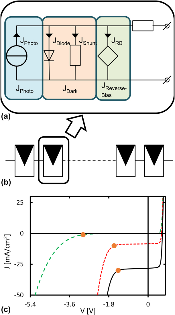
Upon shading, local shunts are formed in regions that have been exposed to a reverse bias voltage. To explain the origin of the reverse bias, the reverse bias behavior of a single cell will be described first. Figures 1(a) and 1(b) show the equivalent circuit of a CIGS solar cell and the graphical representation of the position of one cell in a string of cells within a module, respectively. The light-generated current (blue) varies linearly with light intensity, while the dark current (orange) is the sum of the diode current and the parasitic current through the shunt resistance. The combined contribution of the photo (J _Photo) and dark (J _Dark) current dominates the JV curve at positive voltages, as can be seen in the JV graph of Fig. 1(c). At negative voltages (reverse bias), there is a third contribution [Reference Sun, Raguse, Garris, Deline, Silverman and Alam11] that, besides the shunt resistance, dominates the JV curve, indicated with reverse bias current (J _Reverse-Bias) in Fig. 1 green. For CIGS solar cells, this element is responsible for the rapid increase in current at negative voltages. The onset of this increase is the transition voltage (V _tr) and is indicated with an orange dot in the JV curves in Fig. 1(c). The transition voltage is an indication of the voltage at which the solar cell transits from an isolating nature to a conducting nature. The reverse characteristic, which is the JV curve at negative voltages, is dominated by the transition and depends strongly on both temperature and illumination. It can be influenced by many parameters which will be discussed in a later section. For better readability, all current and voltage values will be treated as absolute numbers, e.g., a change in the transition voltage from 3 to 2 V will be called a reduction of V _tr.

Figure 1:

(a) Equivalent circuit of single cell and (b) representation of this cell in a string of cells as found in a PV module. (c) JV characteristic at different illumination intensities of a single cell. The black solid, red dotted, and green dashed lines represent 1 sun, 0.3 sun, and dark conditions, respectively. The transition voltage (V _tr) is in each curve marked with an orange dot. Measurements performed on a standard cell, fabricated, and measured at the Solliance facilities.

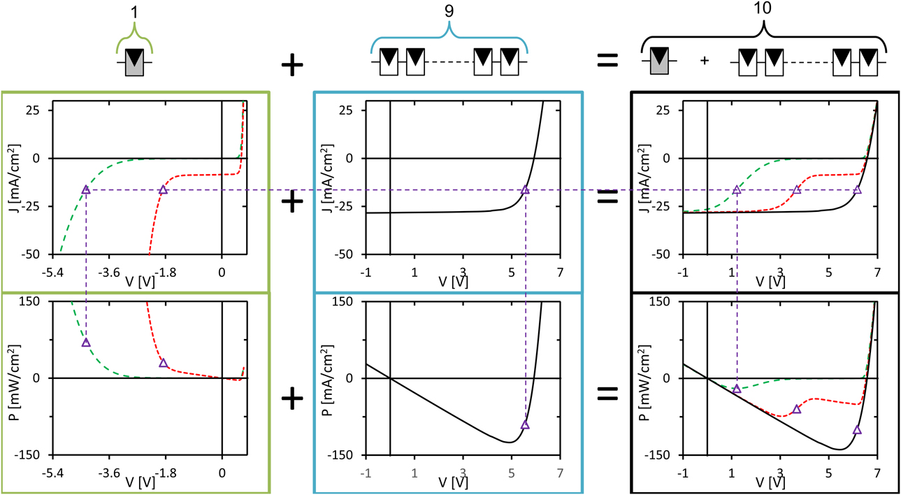
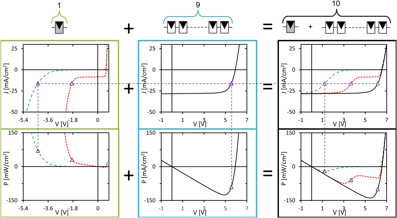
The reverse characteristics of the individual cells in a module determine the internal distribution of voltage and current because a module consists of a string of series connected solar cells. For the example given in Fig. 2, shading is simulated in one cell in a string of ten. The purple dashed line gives the electrical condition at the maximum power point of the constructed JV with nine unshaded and one fully shaded cell. A negative power means that the device is generating energy, while a positive power implies that the device is dissipating energy. Due to the series connection of all cells, the current must be equal in all cells. When the constructed module is operating at the current indicated by the purple dashed line the constructed module is still delivering energy through the external load (negative power in the graph). This energy is supplied by the nine unshaded cells, and the shaded cell is forced to operate at a negative voltage, thus dissipating the majority of the energy generated by the nine unshaded cells. The magnitude of the dissipation can be altered when the reverse bias characteristic of the cell can be influenced.

Figure 2:

Constructed JV curve representing a module with 9 unshaded cells in series with 1 shaded cell. The graphs at the top are JV curves and the graphs at the bottom are PV curves. On the left the JV and PV curves are plotted of 1 cell at different illumination intensities, the red dotted and green dashed lines represent respectively 0.3 sun and dark conditions. The JV and PV graphs in the middle are constructed from a 1 sun illuminated curve; here, the voltage is multiplied by 9 to get the equivalent JV curve of 9 unshaded cells in series. The graphs on the right are the sum of the graphs of the partly shaded cell and the nine unshaded cells together with (black) an unshaded 10 cell module. The purple symbols represent operating points based on the at the maximum power point current of the constructed module with 1 dark and 9 illuminated cells. The construction is based on JV measurements at different illumination intensities of one-standard cell. This cell was fabricated and characterized at the Solliance facilities in Eindhoven, The Netherlands.

Different scenarios for shading tests

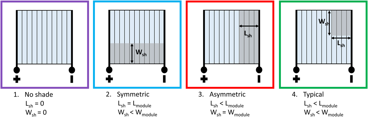
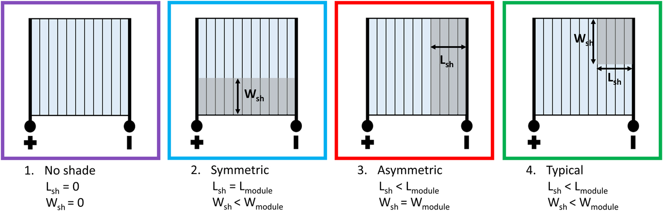
In the field, shading can have any arbitrary form or intensity. Since not every thinkable shadow can be tested, Dongaokar et al. [Reference Dongaonkar, Deline and Alam12] introduced several shading scenarios for testing partial shading in monolithically interconnected thin-film modules. The layouts of the shading masks for these scenarios are depicted in Fig. 3. Almost all reported shading tests can be categorized with these mask layouts, except for diagonal shading or shades that mimic a human body.

Figure 3:

Different shading scenarios as introduced by Donaonkar et al. [Reference Dongaonkar, Deline and Alam12].

Besides the shape of the shading mask, also the opacity of the shading mask is an important parameter. Sometimes, a less opaque mask is used to simulate more realistic conditions: a shadow cast by a distant object, during clear sky conditions, blocks approximately 90% of the incident light. Furthermore, shading tests are always executed under an electrical load or at short circuit conditions. Internal currents will flow as a result of externally extracted current from a partial shaded module, which causes internal power flow in the device under test. This can be large enough to cause permanent damage. At open circuit conditions, no current and power is drawn from the device, so no internal power flow is present.

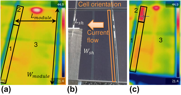
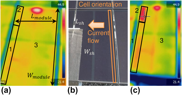
Local differences in operating parameters are expected for each of the shading scenarios, which are listed in Table I. Scenario 1 represents the normal operating condition with no shade. In case of symmetric shading (scenario 2), power generation of each cell is reduced equally and current and voltage in the shaded regions are uniformly reduced. In the third scenario (asymmetric shading), electrical energy is dissipated in the shaded region because the photo-generated current is forced through the shaded cells. This results in a negative (or reverse) operating voltage of the shaded cells. During typical shading (scenario 4), an additional effect of unequal current distribution acts on the top of the stresses in scenarios 2 and 3. Since the effects are strongest when combined with reverse bias conditions, most shading tests are performed with L _sh ≪ W _sh, and this is, unless otherwise stated, the operating condition when referring to the “typical” condition. An example of the temperature distribution for the typical scenario on a module during a field test can be seen in Fig. 4.

TABLE I:

Expected local operating parameters for the different shading conditions. Parameters are based on the authors’ interpretation of Refs. Reference Sun, Raguse, Garris, Deline, Silverman and Alam11, Reference Silverman, Deceglie, Sun, Garris, Alam, Deline and Kurtz18, and Reference Carolus, Purohit, Vandenbergh, Meuris and Tripathi20.

Abbreviations used are Imp: current at maximum power point, Vmp: voltage at maximum power point, OT: operating temperature, NA: not applicable, RB: reverse bias.

Figure 4:

Outdoor measurements of a partial shaded CIGS (Shell Eclipse-80) module. (a) IR picture of module under normal operating condition. The hotspot on top of the module is due to the connectors that caused local heating. (b) Optical picture of module during shading test, with indications of current flow and cell orientation. (c) IR picture directly after the shading test. In (a) and (c) the regions of interest are numbered and indicated. A partly transparent shading mask was applied on region 1. The nonshaded region (Region 2) of the shaded cells exhibit elevated temperatures due to the shading experiment. (Reprinted with permission from Ref. Reference Dongaonkar, Deline and Alam12.)

Shading tests on modules

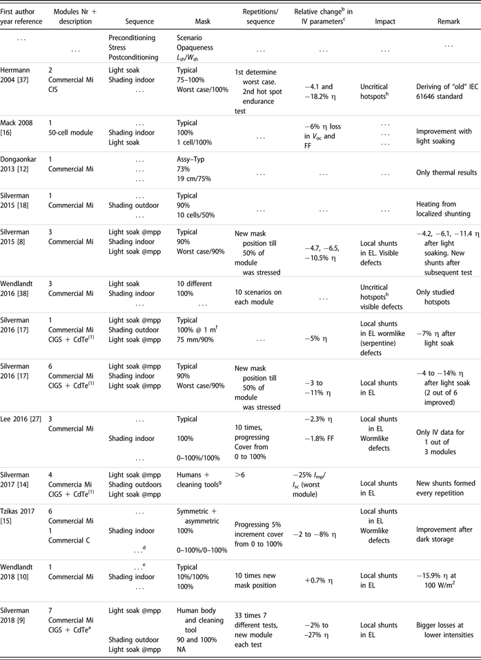
Several studies have been published on shading tests performed on monolithically interconnected CIGS modules. A list of them can be found in Table II. Comparing results presented in the existing literature is challenging due to the following reasons:

1. (i) Lack of uniformity in measurement conditions.

2. (ii) Most sources report on tests executed on only one module or on a comparison of single modules from different types.

3. (iii) Module manufacturers and types are often anonymized.

4. (iv) Changes in efficiency and other electrical parameters are not always mentioned.

5. (v) Large effect of metastabilities and pre-conditioning on module performance [Reference Silverman, Deceglie, Deline and Kurtz8]. It is known that light soaking, electrical biases, and module temperature can temporarily influence the module performance [Reference Gostein and Dunn13]. Therefore, separation of the permanent effects of the partial shading tests and the temporary effects, which are often independent of the partial shading, is very complicated.

TABLE II:

List of available literature that describes shading tests on CIGS modules.

Abbreviations used: L _sh and W _sh: length and width of shading mask, respectively, according to Fig. 3, Mi: monolithically interconnected, C: nonmonolithically interconnected, T _mod: module temperature, CIS: CuInSe₂, I _sc: short circuit current, Imp: current at maximum power point, η: efficiency, V _oc: open circuit voltage, FF: fill factor.

^a Data were anonymized in such a way that the distinction between CIGS and CdTe could not be made.

^b Loss in parameters are relative to before application of stress. For example −10% η means that a module went from an efficiency of 20% before the test to an efficiency of 18% after the test.

^c IV parameters at standard test conditions. If also low light measurements were performed, this is indicated in the last column.

^d Tzikas et al. [Reference Tzikas, Gomez, van den Donker, Bakker, Smets and Folkerts15] also measured IV after several weeks of dark storage.

^e Wendlandt et al. [Reference Wendlandt and Podlowski10] started with stabilized modules.

^f Silverman et al. [Reference Silverman, Mansfield, Repins and Kurtz17] used a 100% opaque mask at a distance of 1 m outdoor that was moved in such a way that the shadow passed over the full width of the module in 20 s.

^g Silverman et al. [Reference Silverman and Ingrid14], tested the influence of real humans and cleaning tools (no artificial masks).

^h In c-Si modules often breakage of glass and melting of encapsulant has been observed; therefore, a noncritical hotspot does not generate sufficient heat to break the glass or melt the encapsulant.

Besides the challenges, the main observation is that after shading tests, modules displayed a reduced efficiency, which is accompanied by the formation of local shunts. In all publications from 2015 till present (Table II), local shunts are described, which are commonly linked to the following observations:

1. (i) Reduction of module efficiency due to a reduced fill factor, associated with local shunts.

2. (ii) The formation of shunts is a very fast process, and hence, defects can form within one 10-ms single flash IV measurement [Reference Wendlandt and Podlowski10] or after several 100-ms flashes [Reference Silverman, Deceglie, Deline and Kurtz8].

3. (iii) The occurrence of shunts does not stop with consecutive measurements, the damage adds up after each new stress exposure [Reference Silverman and Repins9, Reference Silverman and Ingrid14]. The impact on module performance can, therefore, become severe, even though the individual effects of stress exposure are sometimes small.

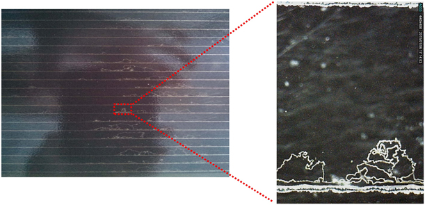
4. (iv) The defects causing the shunts are often referred to as wormlike defect, due to their distinct visual appearance. An example of the typical appearance of wormlike defects after a shading test can be found in Fig. 5. More information on these defects is presented in a later section.

5. (v) The wormlike defects form in the region where a reverse bias voltage was present.

Figure 5:

Pictures of wormlike defects in a CIGS module after shading stress test. (Reprinted with permission from Ref. Reference Lee, Bae, Oh, Park, Kim, Lee, Nam, Bin Mo, Kim, Yang, Kang, Lee and Kim27.)

Another observation is that shading test lead to an initial change in performance, which is not stable over time. Some authors observed recovery after dark storage [Reference Tzikas, Gomez, van den Donker, Bakker, Smets and Folkerts15] or light soaking [Reference Mack, Walter, Kniese, Hariskos and Schäffler16], but also mixed results were found with both improving and degrading modules after light stabilization treatment [Reference Silverman, Deceglie, Deline and Kurtz8, Reference Silverman, Mansfield, Repins and Kurtz17].

Thermoelectrical models on CIGS cells and modules

To estimate the stress loads during partial shading events, it is important to predict the internal voltage, current, and temperature profiles. Thermoelectrical modeling can, therefore, be used to explain the temperature differences during shading events, as would occur in the field (Fig. 4). Specific models that are developed for CIGS devices have to take into account the nonlinear dependency of the reverse curve on illumination. This mechanism is responsible for the internal electrical current flow that is preferential in the illuminated area [Reference Silverman, Deceglie, Sun, Garris, Alam, Deline and Kurtz18]. The following thermoelectrical models and how they included the light dependency for CIGS devices have been published:

1. (i) Sun et al. [Reference Sun, Raguse, Garris, Deline, Silverman and Alam11] introduced the Poole–Frenkel mechanism to account for the light dependency of the reverse characteristic. The model uses a 2D SPICE simulation. The Poole–Frenkel principle was verified with the aid of cell measurements from another publication [Reference Szaniawski, Lindahl, Törndahl, Zimmermann and Edoff19].

2. (ii) Silverman et al. [Reference Silverman, Deceglie, Sun, Garris, Alam, Deline and Kurtz18], used the Poole–Frenkel mechanism introduced by Sun et al. [Reference Sun, Raguse, Garris, Deline, Silverman and Alam11]. They validated the thermoelectrical model with temperature measurements on a commercial module. The model utilizes commercial Finite Element Analyses software.

3. (iii) Carolus et al. [Reference Carolus, Purohit, Vandenbergh, Meuris and Tripathi20], also used a thermoelectrical 2D SPICE model. The light dependency is accounted for by the use of measured JV curve both in the dark and under illumination. Verification of their model is a work in progress that has not yet been published.

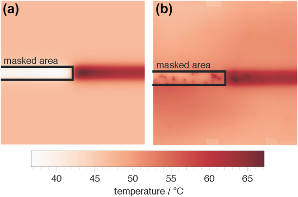
Predictions do not always match reality as was shown by Silverman et al. [Reference Silverman, Deceglie, Sun, Garris, Alam, Deline and Kurtz18] who compared the modeled and actual temperature data (Fig. 6). The model correctly predicted an increase in temperature for the noncovered parts of the partly masked cells. However, their measurements showed small hotspots in both the covered and noncovered parts of the partly masked cells. These hotspots originate from already existing local shunts as well as the formation of new reverse bias induced defects. This type of defects has been successfully predicted by Nardone et al. [Reference Nardone, Dahal and Waddle21], who included local weak spots in their model. These weak spots consumed all current in the shaded cells, causing local heating.

Figure 6:

Simulated and measured maps of the back of the module temperature. The area inside the black line is the shaded area. (a) Simulation results of 100 cells in a 0.5 × 0.5 m module. (b) Measurement of 0.6 × 0.6 m portion of a larger commercial module. (Reprinted with permission from Ref. Reference Silverman, Deceglie, Sun, Garris, Alam, Deline and Kurtz18.)

Reverse bias induced defects

In a module, the reverse bias induced defects act as local shunts and are often referred to as wormlike defects due to their distinct visual appearance. The first observation in 2007 was by van Dyk et al. [Reference van Dyk, Radue and Gxasheka22]; however, they did not name them wormlike defects or linked them with the exposure to reverse bias. Introduction of the term wormlike defect came from Westin et al. [Reference Westin, Zimmermann, Stolt and Edoff23] in 2009. Some descriptions that have been given on the origin and nature of the wormlike defects are follows:

1. (i) Formation has been observed as being a moving hotspot that moves toward the P1 scribe, while propagation along the P1 scribe is also observed [Reference Westin, Zimmermann, Stolt and Edoff23, Reference Johnston, Palmiotti, Gerber, Guthrey, Mansfield, Silverman, Al-Jassiml and Rockett24, Reference Palmiotti, Johnston, Gerber, Guthrey, Rockett, Mansfield, Silverman and Al-Jassim25, Reference Johnston, Sulas, Palmiotti, Gerber, Guthrey, Liu, Mansfield, Silverman, Rockett and Al-Jassim26].

2. (ii) The origin is often an already existing weak spot like a small shunt [Reference Johnston, Palmiotti, Gerber, Guthrey, Mansfield, Silverman, Al-Jassiml and Rockett24, Reference Palmiotti, Johnston, Gerber, Guthrey, Rockett, Mansfield, Silverman and Al-Jassim25, Reference Johnston, Sulas, Palmiotti, Gerber, Guthrey, Liu, Mansfield, Silverman, Rockett and Al-Jassim26].

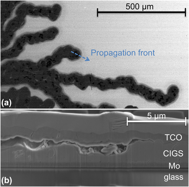
3. (iii) The absorber material has changed into a very porous structure [Reference Westin, Zimmermann, Stolt and Edoff23, Reference Palmiotti, Johnston, Gerber, Guthrey, Rockett, Mansfield, Silverman and Al-Jassim25, Reference Lee, Bae, Oh, Park, Kim, Lee, Nam, Bin Mo, Kim, Yang, Kang, Lee and Kim27] leading to changes in both composition and electronic properties. An example of the changed electronic properties is shown in the electron beam induced current (EBIC) image of Fig. 7(a).

4. (iv) Large voids have been found at the interface of the transparent conductive oxide (TCO) and the CIGS material, as can be seen in Fig. 7(b). Lifting the TCO layer gives the signature appearance [Reference Westin, Zimmermann, Stolt and Edoff23, Reference Palmiotti, Johnston, Gerber, Guthrey, Rockett, Mansfield, Silverman and Al-Jassim25].

5. (v) The composition inside the defects has changed; zinc from the aluminum-doped zinc oxide TCO has been found to migrate into the CIGS absorber, while copper migrated toward the back contact. Brighter areas that have been found in SEM cross-section are believed to be phase segregations [Reference Westin, Zimmermann, Stolt and Edoff23].

Figure 7:

(a) EBIC picture of wormlike defect. Brighter colors represent more efficient current collection. The wormlike defect appears darker in this image, meaning that the defect has completely different electronic properties. (b) Cross-section of wormlike defect prepared with focused ion beam (FIB). Large voids have been formed at the TCO–CIGS interface. (Reprinted with permission from Ref. Reference Palmiotti, Johnston, Gerber, Guthrey, Rockett, Mansfield, Silverman and Al-Jassim25.)

Regardless of these studies, many questions about the origin and propagation mechanisms of these wormlike defects still exist. Explanations using thermoelectrical models are contradictory. Richter et al. [Reference Richter, Neerken and Parisi28] concluded that neither diode-like defects nor ohmic shunts could generate sufficient heat to cause irreversible damage. Nardone et al. [Reference Nardone, Dahal and Waddle21] on the other hand calculated that the current density in a local weak spot can reach approximately 10⁸ A/m [Reference Birant, de Wild, Meuris, Poortmans and Vermang2], with accompanying peak temperatures above 900 K, enough to cause permanent material damage.

Experimental evidence exists that the wormlike defects originate in local weak spots like shunts [Reference Johnston, Palmiotti, Gerber, Guthrey, Mansfield, Silverman, Al-Jassiml and Rockett24, Reference Palmiotti, Johnston, Gerber, Guthrey, Rockett, Mansfield, Silverman and Al-Jassim25, Reference Johnston, Sulas, Palmiotti, Gerber, Guthrey, Liu, Mansfield, Silverman, Rockett and Al-Jassim26]. However, Richter et al. [Reference Richter and Vrenegor29] showed by using statistical analyses that the formation of wormlike defects is likely driven by an electric field rather than high local currents associated with local defects. The results from Richter et al. [Reference Richter and Vrenegor29] are in line with the results from Puttnins et al. [Reference Puttnins, Jander, Pelz, Heinker, Daume, Rahm, Braun and Grundmann30], who found a lower chance of forming wormlike defects when a thicker TCO was used.

Reverse characteristic of single cells

One of the means to prevent reverse bias induced defects from forming is to limit the reverse bias voltage over a cell. This can be achieved by alternating the reverse characteristic in such a way that it acts as a build-in bypass diode. This requires a good understanding of the mechanisms behind the transition. Therefore, several studies have been performed on the reverse characteristic [Reference Mack, Walter, Kniese, Hariskos and Schäffler16, Reference Silverman, Mansfield, Repins and Kurtz17, Reference Silverman, Deceglie, Sun, Garris, Alam, Deline and Kurtz18, Reference Szaniawski, Lindahl, Törndahl, Zimmermann and Edoff19, Reference Puttnins, Jander, Pelz, Heinker, Daume, Rahm, Braun and Grundmann30, Reference Puttnins, Jander, Wehrmann, Benndorf, Stölzel, Müller, von Wenckstern, Daume, Rahm and Grundmann31, Reference Szaniawski, Zabierowski, Olsson, Zimmermann and Edoff32, Reference Puttnins, Purfurst, Hartung, Lee, Daume, Hartmann, Rahm, Braun and Grundmann33].

A uniform description of the reverse characteristic is needed to be able to reliably compare studies from different sources. Unfortunately, the shape of the reverse characteristic has not been described thoroughly, which is in contrast with the forward region of the JV curve. Here, the shape of the curve can be described by the combination of 5 parameters (V _oc, I _sc, FF, R _shunt, and R _series). The shape of the reverse characteristic seems more complex and is less studied. Often, one characteristic point on the reverse bias curve is used to compare samples within a study. The transition voltage is one of these points used to compare reverse characteristics. Two different approaches for the determination of the transition voltage have been published [Reference Puttnins, Jander, Wehrmann, Benndorf, Stölzel, Müller, von Wenckstern, Daume, Rahm and Grundmann31, Reference Szaniawski, Zabierowski, Olsson, Zimmermann and Edoff32]. A more empiric method to compare the shapes of different reverse characteristics is to use the voltage needed to drive either a fixed current [Reference Silverman, Mansfield, Repins and Kurtz17] (30 mA/cm² in the dark and 70 mA/cm² under illumination) or the photocurrent [Reference Mack, Walter, Kniese, Hariskos and Schäffler16].

Several publications have reported on the influence of external conditions, like illumination intensity, spectrum of the light source, and temperature, on the reverse characteristic. The reported trends include the following:

1. (i) A shift in transition voltages with illumination intensity [Reference Mack, Walter, Kniese, Hariskos and Schäffler16, Reference Silverman, Deceglie, Sun, Garris, Alam, Deline and Kurtz18, Reference Puttnins, Jander, Wehrmann, Benndorf, Stölzel, Müller, von Wenckstern, Daume, Rahm and Grundmann31]: a higher light intensity leads to a reduction in V _tr.

2. (ii) Influence of the spectrum of the illumination source on the transition voltage. Several sources [Reference Mack, Walter, Kniese, Hariskos and Schäffler16, Reference Szaniawski, Lindahl, Törndahl, Zimmermann and Edoff19, Reference Puttnins, Jander, Wehrmann, Benndorf, Stölzel, Müller, von Wenckstern, Daume, Rahm and Grundmann31] reported that high energetic blue illumination reduces the transition voltage, while illumination with low energetic (red) light more resembled the behavior in the dark.

3. (iii) The transition voltage increases when the temperature is reduced [Reference Szaniawski, Lindahl, Törndahl, Zimmermann and Edoff19, Reference Puttnins, Jander, Wehrmann, Benndorf, Stölzel, Müller, von Wenckstern, Daume, Rahm and Grundmann31]. However, there seems to be a local maximum in the transition voltage around 200 K which depends on illumination wavelength [Reference Puttnins, Jander, Wehrmann, Benndorf, Stölzel, Müller, von Wenckstern, Daume, Rahm and Grundmann31]. Below this temperature, the transition voltage reduces again.

Besides external factors, the composition of the solar cell also influences the reverse characteristics; some reported compositional influences are as follows:

1. (i) Effects of the buffer layer;

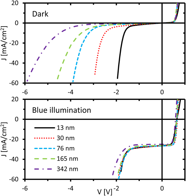
   1. (a) The buffer layer thickness influences the transition voltage, a thicker buffer layer leads to a higher transition voltage in the dark [Reference Szaniawski, Lindahl, Törndahl, Zimmermann and Edoff19, Reference Puttnins, Jander, Pelz, Heinker, Daume, Rahm, Braun and Grundmann30]. This is, however, not the case when illuminated with blue light [Reference Szaniawski, Lindahl, Törndahl, Zimmermann and Edoff19], as is shown in Fig. 8 for cells with a ZnSnO (ZTO) buffer layer with varying thickness.

   2. (b) No influence of the buffer layer material. Cells with CdS and ZTO layers show the same behavior both in the dark [Reference Szaniawski, Lindahl, Törndahl, Zimmermann and Edoff19, Reference Szaniawski, Zabierowski, Olsson, Zimmermann and Edoff32] and with blue illumination [Reference Szaniawski, Lindahl, Törndahl, Zimmermann and Edoff19].

2. (ii) A higher sodium concentration in the CIGS layer reduces the transition voltage [Reference Puttnins, Jander, Wehrmann, Benndorf, Stölzel, Müller, von Wenckstern, Daume, Rahm and Grundmann31, Reference Puttnins, Purfurst, Hartung, Lee, Daume, Hartmann, Rahm, Braun and Grundmann33].

3. (iii) The influence of the TCO layer thickness on the reverse characteristic is very small; however, a thicker TCO layer dramatically improved the survival rate of the cells from 25 to 75% [Reference Puttnins, Jander, Pelz, Heinker, Daume, Rahm, Braun and Grundmann30].

4. (iv) The reverse characteristic reduces when the absorber layer thickness is reduced [Reference Silverman, Mansfield, Repins and Kurtz17].

Figure 8:

Influence of buffer layer thickness on both dark and (blue) illuminated JV curves. The top graph shows JV measurements in the dark with decreasing transition voltage with increasing buffer layer thickness (thickness increase from black solid to purple dashed dotted curve). Bottom graph shows JV measurements of the same cells with blue illumination. (Reprinted with permission from Ref. Reference Szaniawski, Lindahl, Törndahl, Zimmermann and Edoff19.)

The observed trends are the basis of speculation on the mechanism behind the transition. Based on similarities with traditional semiconductor physics, the main mechanisms discussed are impact ionization (avalanche effect) or tunneling (Zener effect). Although also other tunneling mechanism (Poole–Frenkel and Fowler–Nordheim) have been considered specifically for CIGS devices. The suggested mechanisms in chronological order of publication are as follows:

1. (i) Mack et al. [Reference Mack, Walter, Kniese, Hariskos and Schäffler16] concluded that the transition in the dark could be caused by either tunneling or avalanche currents, and the process is likely assisted by metastable interface charges.

2. (ii) Szaniawski et al. [Reference Szaniawski, Lindahl, Törndahl, Zimmermann and Edoff19] concluded that under illumination, tunneling is the exclusive mechanism behind the transition. However, in the dark, it could be either tunneling or a combination of tunneling and avalanching.

3. (iii) Puttnins et al. [Reference Puttnins, Jander, Wehrmann, Benndorf, Stölzel, Müller, von Wenckstern, Daume, Rahm and Grundmann31] argued that in dark, it could be either tunneling or a combination of tunneling and avalanching.

4. (iv) Silverman et al. [Reference Silverman, Deceglie, Sun, Garris, Alam, Deline and Kurtz18] together with Sun et al. [Reference Sun, Raguse, Garris, Deline, Silverman and Alam11] introduced the Poole–Frenkel mechanism to account for the observed differences between dark and illumination behavior.

5. (v) Nardone et al. [Reference Nardone and Dahal34] showed with semiconductor physic device simulations that the conventional mechanisms (including Poole-Frenkel) cannot adequately describe the reverse characteristic of CIGS cells.

6. (vi) Szaniawski et al. [Reference Szaniawski, Zabierowski, Olsson, Zimmermann and Edoff32] introduced the Fowler–Nordheim tunneling as the dominant mechanism in the dark.

Over time, the more traditional Zener and avalanche mechanisms have been replaced by more complicated tunneling mechanisms. However, the mechanisms proposed do not fully explain the observed difference between the behavior under illumination and in the dark. The key in understanding the reverse characteristic of CIGS cells would be a mechanism that explains the discrepancy between light and dark. The Poole–Frenkel mechanism [Reference Sun, Raguse, Garris, Deline, Silverman and Alam11, Reference Silverman, Deceglie, Sun, Garris, Alam, Deline and Kurtz18] could provide such an explanation. However, it was proven both experimentally [Reference Szaniawski, Zabierowski, Olsson, Zimmermann and Edoff32] and theoretically [Reference Nardone and Dahal34] that the Poole–Frenkel mechanism is probably not responsible for the transition in the dark. So, despite all the efforts, there is still more research needed to fully understand the mechanism behind the reverse characteristic.

Nonpermanent effects

While the formation of wormlike defects likely has the largest effect on device performance, various other effects have also been observed on single cells or small research modules:

1. (i) Mack et al. (2008) [Reference Mack, Walter, Kniese, Hariskos and Schäffler16], observed metastabilities caused by illumination and annealing at 160 °C in the dark. Light soaking and annealing reduces and increases the transition voltage, respectively.

2. (ii) Westin et al. (2008) [Reference Westin, Zimmermann, Stolt and Edoff23] observed degradation of V _oc and FF after combined exposure of cells to illumination and reverse bias. This was in contrast to cells that were only exposed to reverse bias in the dark, which only showed a reduction of the FF. They also reported that degradation of the V _oc could be recovered by light soaking.

3. (iii) Szaniawski et al. (2013) [Reference Szaniawski, Lindahl, Törndahl, Zimmermann and Edoff19] observed a very slow response of the current to changes in illumination for cells held at a constant negative voltage. In their study, it could take up to 5 min for the current to reach an equilibrium state after changes in illumination were applied.

4. (iv) Szaniawski et al. (2017) [Reference Szaniawski, Zabierowski, Olsson, Zimmermann and Edoff32] observed that the reverse characteristic was shifting when repeating reverse JV measurements. They also described an increase in current over time when a cell is kept at a fixed negative voltage in the dark.

5. (v) Mortazavi et al. (2017) [Reference Mortazavi, Bakker, Carolus, Daenen, de Amorim Soares, Steijvers, Weeber and Theelen35] observed a decrease in JV parameters for cells after a short (1 min) exposure to reverse bias voltages larger than 2 V. They also reported severe damage for cells after long (1 h) exposure to reverse voltages of 1.5 and 2 V, which could partly be recovered by light soaking.

6. (vi) Theelen et al. (2016) [Reference Theelen, Steijvers, Bakker, Vink, Mortazavi, Mulder, Barreau, Roosen and Haverkamp36] observed that during combined damp heat and illumination conditions, cells that were kept at a negative bias degraded more rapidly than the cells held at V _oc, J _sc, or maximum power point over a period of 200 h.