1 Introduction
A sessile droplet on a structured surface characterized by sufficiently small periodic length scales may be stable in the Cassie state, where solid–liquid contact is exclusively at the tips of the structures (Quéré Reference Quéré2005). A liquid flowing over a structured surface may be as well. We assume this here, and the necessary criteria are provided by Lam, Hodes & Enright (Reference Lam, Hodes and Enright2015). The no-slip boundary condition is valid at solid–liquid interfaces, as the corresponding molecular slip lengths are on the scale of 10 nm or less; see, e.g., Huang et al. (Reference Huang, Sendner, Horinek, Netz and Bocquet2008) for values from molecular dynamics simulations and Cottin-Bizonne et al. (Reference Cottin-Bizonne, Steinberger, Cross, Raccurt and Charlaix2008) for those from experiment. However, lubrication is achieved because of the low shear stress at liquid–gas interfaces (menisci). (Normally, there is vapour on account of the vapour pressure of the liquid phase and inert gas adjacent to menisci. We use the term ‘gas’ for brevity.) The apparent hydrodynamic slip length (
 $b$
), subsequently referred to as the slip length, is used to quantify the effect of such lubrication on flow resistance in microfluidic conduits.
Except for the investigations by Baier, Steffes & Hardt (Reference Baier, Steffes and Hardt2010a
,Reference Baier, Steffes and Hardt
b
) discussed below, available results for
 $b$
apply to adiabatic flows. We summarize those for parallel (streamwise) ridges in a laminar flow. Ybert et al. (Reference Ybert, Barentin, Cottin-Bizonne, Joseph and Bocquet2007) provide a set of scaling laws for
 $b$
that are consistent with their numerical results and capture the oft-neglected effects of shear stress exerted on the liquid phase by the gas phase, meniscus curvature and molecular slip at solid–liquid interfaces. Such effects were not considered in the studies discussed below unless noted.
Lauga & Stone (Reference Lauga and Stone2003) provide an expression for
 $b$
based upon the results of Philip (Reference Philip1972a
,Reference Philip
b
) for Poiseuille flow through a circular tube. For the parallel-plate geometry, when one plate is textured and the other is smooth, Sbragaglia & Prosperetti (Reference Sbragaglia and Prosperetti2007) computed the slip length as a function of ridge width to ridge pitch ratio (solid fraction) and channel spacing to ridge pitch ratio. This was done by numerically solving a set of dual series equations resulting from an eigenfunction expansion and follows from other results by Philip (Reference Philip1972a
,Reference Philip
b
), as discussed in § 3.3. Teo & Khoo (Reference Teo and Khoo2009) considered the additional case of a symmetrically textured parallel-plate channel using the same technique, as did Kirk, Hodes & Papageorgiou (Reference Kirk, Hodes and Papageorgiou2017). In the limit where the height of the channel is large compared with the ridge pitch, the aforementioned studies show that the slip length non-dimensionalized by the ridge pitch is the same as that for the circular tube geometry.
Maynes et al. (Reference Maynes, Jeffs, Woolford and Webb2007) semianalytically and experimentally studied Poiseuille flow through a symmetrically textured parallel-plate channel. The coupled velocity profiles in the liquid (water at standard conditions) and gas (air at standard conditions) phases were computed. It was shown that interfacial shear can substantially reduce the slip length. For example, at a solid fraction of 0.031, ridge pitch to hydraulic diameter ratio of 1 and cavity depth to hydraulic diameter ratio of 0.1, the slip length is reduced by nearly 50 % relative to the shear-free meniscus case. Experimental data obtained by Maynes et al. (Reference Maynes, Jeffs, Woolford and Webb2007) are reasonably consistent with their predictions and exhibit the same trends. Ng, Chu & Wang (Reference Ng, Chu and Wang2010) considered the additional effect of intrinsic slip at solid–liquid interfaces and reduced the computational effort required to compute the slip length by using eigenfunction expansions to avoid the use of a brute-force numerical approach for the gas-phase portion of the domain. Lee, Choi & Kim (Reference Lee, Choi and Kim2008) measured slip lengths for a surface with concentric parallel ridges in a Couette flow using a cone and plate rheometer, and their results were consistent with theoretical predictions. Finally, Sbragaglia & Prosperetti (Reference Sbragaglia and Prosperetti2007) utilized a boundary perturbation to capture the effects of (small) meniscus curvature on slip length in their aforementioned study, as did Kirk et al. (Reference Kirk, Hodes and Papageorgiou2017) when both walls rather than one wall of a parallel-plate channel are textured. When the meniscus bows into the cavity and the liquid, the slip length is increased and decreased respectively, on account of the change in the cross-sectional area of the liquid domain. However, the velocity field is also perturbed, and the net result may be an increase or decrease in the slip length for either direction of meniscus deflection.
In the case of an unbounded shear flow with a periodic array of parallel ridges, the slip length follows from the results of Philip (Reference Philip1972a ). When non-dimensionalized by ridge pitch, it is identical to that obtained for Poiseuille flow through a circular tube. Crowdy (Reference Crowdy2011) extended this flow configuration to an arbitrary pattern of no shear slots in each periodic window along with an arbitrary ridge orientation relative to the flow direction using numerically computed Schottky–Klein prime functions. Moreover, by utilizing a series of conformal maps, Crowdy (Reference Crowdy2010) captured the effects of arbitrary (constant) meniscus curvature on the slip length in the high-solid-fraction limit. Additionally, Teo & Khoo (Reference Teo and Khoo2010) numerically computed slip lengths for Couette and Poiseuille (internal) flows over a wide range of geometric parameters including meniscus curvature, and their results are consistent with those of Crowdy (Reference Crowdy2010) at sufficiently high channel height to ridge pitch ratio and solid fraction.
Only Baier et al. (Reference Baier, Steffes and Hardt2010a
,Reference Baier, Steffes and Hardt
b
) have considered the effect of thermocapillary stress on slip length. A constant streamwise temperature gradient was imposed along the domain and the slip length for a shear flow was computed utilizing the Lorentz reciprocal theorem. The slip lengths were consistent with those predicted by numerical simulations when the channel height to ridge pitch ratio was 4. It was concluded that by the imposition of temperature gradients of the order of
 $10\,^{\circ }\text{C}~\text{cm}^{-1}$
, water may be pumped through microchannels at mean velocities of the order of several
 $\text{mm}~\text{s}^{-1}$
.
We compute the slip length for a diabatic and fully developed laminar Poiseuille flow through a parallel-plate channel textured on one side with uniform width and pitch parallel ridges. Thermocapillary stress along menisci is accounted for and may be set equal to zero to compute the slip lengths for an adiabatic flow. The problem is specified and the governing equations are developed in § 2. In § 3, under simplifying assumptions, exact and, subsequently, asymptotic solutions are developed. Then, a procedure for the numerical solution of the problem is provided. Results are presented in § 4 and conclusions in § 5.
2 Problem formulation
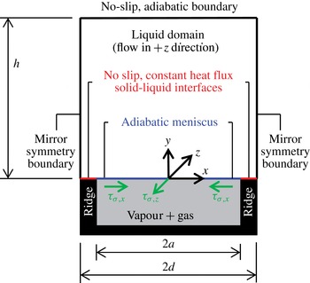
The liquid domain is shown in figure 1. The composite interface corresponds to its
 $y=0$
boundary and includes an adiabatic and flat meniscus and solid–liquid interfaces. The width of the meniscus is
 $2a$
and the pitch of the ridges is
 $2d$
. We note that the assumption of an adiabatic meniscus implies neglect of the velocities induced normal to it by evaporation and condensation (Hodes et al.
Reference Hodes, Lam, Cowley, Enright and MacLachlan2015). Heat is supplied to (or removed from) the liquid through the solid–liquid interfaces, where no-slip and constant heat flux boundary conditions are imposed. Mirror symmetry boundary conditions apply along the sides of the domain at
 $|x|=d$
, and the (flat) top of it at
 $y=h$
is subjected to no-slip and adiabatic boundary conditions. (A mirror symmetry boundary condition may also have been applied at
 $x=0$
.) We note that to minimize the magnitude of the difference between the temperature at a point along the solid–liquid interface and the bulk temperature of the liquid, heat may be exchanged with the solid boundary along the smooth rather than the textured side of the channel, where the surface area for heat transfer (that of the ridge tip) is reduced. Then, however, except when the domain aspect ratio, defined here as half of the ridge pitch (
 $d$
) divided by the domain height (
 $h$
), is large compared with unity, the temperature along the meniscus in the
 $x$
direction is essentially constant. This would preclude us from investigating the effect of transverse thermocapillary stress on slip. It is further noted that, when heat is exchanged exclusively along the smooth side of the channel and the aspect ratio of the domain is small compared with unity, the Stokes flow assumption applies and leads to the exact solutions for the velocity field developed in § 3.2.
Domain and boundary conditions. A streamwise pressure gradient is imposed in the
 $z$
direction.

The directions of the streamwise and transverse thermocapillary stresses acting on the meniscus, i.e.
 $\unicode[STIX]{x1D70F}_{\unicode[STIX]{x1D70E},z}$
and
 $\unicode[STIX]{x1D70F}_{\unicode[STIX]{x1D70E},x}$
respectively, shown in figure 1 assume that the heat flux at the solid–liquid interface (
 $q_{sl}^{\prime \prime }$
) is into the liquid, and the mean flow is in the positive
 $z$
direction (
 $-\unicode[STIX]{x2202}p/\unicode[STIX]{x2202}z>0$
). Then, since surface tension decreases with temperature, the streamwise thermocapillary stress along the meniscus pulls the liquid upstream. In the
 $x$
–
 $y$
plane, the temperature of the meniscus is highest at the triple contact lines and monotonically decreases towards the centre of the domain (
 $x=0$
); consequently, the transverse thermocapillary stresses pull the liquid towards the centre of the meniscus and induce a transverse velocity field.
We assume that the derivative of surface tension with respect to temperature (
 $\text{d}\unicode[STIX]{x1D70E}/\text{d}T$
) is constant and that the thermophysical properties of the liquid are otherwise constant. The relevant forms of the continuity, Navier–Stokes and thermal energy equations are respectively
 $$\begin{eqnarray}\displaystyle & \displaystyle \frac{\unicode[STIX]{x2202}u}{\unicode[STIX]{x2202}x}+\frac{\unicode[STIX]{x2202}v}{\unicode[STIX]{x2202}y}=0, & \displaystyle\end{eqnarray}$$
 $$\begin{eqnarray}\displaystyle & \displaystyle u\frac{\unicode[STIX]{x2202}u}{\unicode[STIX]{x2202}x}+v\frac{\unicode[STIX]{x2202}u}{\unicode[STIX]{x2202}y}=-\frac{1}{\unicode[STIX]{x1D70C}}\frac{\unicode[STIX]{x2202}p}{\unicode[STIX]{x2202}x}+\frac{\unicode[STIX]{x1D707}}{\unicode[STIX]{x1D70C}}\left(\frac{\unicode[STIX]{x2202}^{2}u}{\unicode[STIX]{x2202}x^{2}}+\frac{\unicode[STIX]{x2202}^{2}u}{\unicode[STIX]{x2202}y^{2}}\right), & \displaystyle\end{eqnarray}$$
 $$\begin{eqnarray}\displaystyle & \displaystyle u\frac{\unicode[STIX]{x2202}v}{\unicode[STIX]{x2202}x}+v\frac{\unicode[STIX]{x2202}v}{\unicode[STIX]{x2202}y}=-\frac{1}{\unicode[STIX]{x1D70C}}\frac{\unicode[STIX]{x2202}p}{\unicode[STIX]{x2202}y}+\frac{\unicode[STIX]{x1D707}}{\unicode[STIX]{x1D70C}}\left(\frac{\unicode[STIX]{x2202}^{2}v}{\unicode[STIX]{x2202}x^{2}}+\frac{\unicode[STIX]{x2202}^{2}v}{\unicode[STIX]{x2202}y^{2}}\right), & \displaystyle\end{eqnarray}$$
 $$\begin{eqnarray}\displaystyle & \displaystyle u\frac{\unicode[STIX]{x2202}w}{\unicode[STIX]{x2202}x}+v\frac{\unicode[STIX]{x2202}w}{\unicode[STIX]{x2202}y}=-\frac{1}{\unicode[STIX]{x1D70C}}\frac{\unicode[STIX]{x2202}p}{\unicode[STIX]{x2202}z}+\frac{\unicode[STIX]{x1D707}}{\unicode[STIX]{x1D70C}}\left(\frac{\unicode[STIX]{x2202}^{2}w}{\unicode[STIX]{x2202}x^{2}}+\frac{\unicode[STIX]{x2202}^{2}w}{\unicode[STIX]{x2202}y^{2}}\right), & \displaystyle\end{eqnarray}$$
 $$\begin{eqnarray}\displaystyle & \displaystyle u\frac{\unicode[STIX]{x2202}T}{\unicode[STIX]{x2202}x}+v\frac{\unicode[STIX]{x2202}T}{\unicode[STIX]{x2202}y}+w\frac{\unicode[STIX]{x2202}T}{\unicode[STIX]{x2202}z}=\unicode[STIX]{x1D6FC}\left(\frac{\unicode[STIX]{x2202}^{2}T}{\unicode[STIX]{x2202}x^{2}}+\frac{\unicode[STIX]{x2202}^{2}T}{\unicode[STIX]{x2202}y^{2}}\right), & \displaystyle\end{eqnarray}$$
where
 $u$
,
 $v$
and
 $w$
are the velocity components in the
 $x$
,
 $y$
and
 $z$
directions respectively and
 $\unicode[STIX]{x1D70C}$
,
 $\unicode[STIX]{x1D707}$
and
 $\unicode[STIX]{x1D6FC}$
are the density, viscosity and thermal diffusivity respectively of the liquid. As per the hydrodynamically fully developed flow assumption, we have ignored terms containing partial derivatives of velocities with respect to
 $z$
. Additionally, we do not consider variations in the radius of curvature along the meniscus due to the streamwise pressure gradient along the channel or dependence of the surface tension on temperature. Thus,
 $\unicode[STIX]{x2202}p/\unicode[STIX]{x2202}z$
is a prescribed constant. We note that in the thermal energy equation, axial conduction is absent on account of the fully developed assumption and constant heat flux boundary condition (see, e.g., Papoutsakis, Ramkrishna & Lim Reference Papoutsakis, Ramkrishna and Lim1980), and viscous dissipation is assumed to be negligible.
The temperature field varies linearly in the
 $z$
direction for thermally fully developed flow; therefore,
 $\unicode[STIX]{x2202}T/\unicode[STIX]{x2202}z$
equals the axial gradient in mean temperature (Bergman et al.
Reference Bergman, Incropera, DeWitt and Lavine2011). Hence, a macroscopic energy balance on a
 $2d\times h\times \text{d}z$
control volume yields
 $$\begin{eqnarray}\frac{\unicode[STIX]{x2202}T}{\unicode[STIX]{x2202}z}=\frac{2q_{sl}^{\prime \prime }(d-a)}{\unicode[STIX]{x1D70C}Qc_{p}},\end{eqnarray}$$
where
 $Q$
is the volumetric flow rate of liquid through the domain, i.e.
 $2\bar{w}hd$
, where
 $\bar{w}$
is the mean velocity of the liquid and
 $c_{p}$
is its specific heat at constant pressure.
At
 $x=|d|$
, the mirror symmetry boundary condition manifests itself as
 $\unicode[STIX]{x2202}v/\unicode[STIX]{x2202}x=\unicode[STIX]{x2202}w/\unicode[STIX]{x2202}x=\unicode[STIX]{x2202}T/\unicode[STIX]{x2202}x=\unicode[STIX]{x2202}p/\unicode[STIX]{x2202}x=u=0$
. (In the presence of transverse thermocapillary stress, at
 $x=|d|$
,
 $\unicode[STIX]{x2202}u/\unicode[STIX]{x2202}x\neq 0$
, i.e.
 $u$
is an odd function, whereas
 $v$
,
 $w$
,
 $p$
and
 $T$
are even ones.) Moreover,
 $u$
,
 $v$
,
 $w$
and
 $\unicode[STIX]{x2202}T/\unicode[STIX]{x2202}y$
equal 0 at
 $y=h$
. At the composite interface (
 $y=0$
),
 $u=0$
for
 $a<|x|<d$
and an interfacial (
 $x$
direction) stress balance yields
 $\unicode[STIX]{x1D707}(\unicode[STIX]{x2202}u/\unicode[STIX]{x2202}y+\unicode[STIX]{x2202}v/\unicode[STIX]{x2202}x)=-(\unicode[STIX]{x2202}T/\unicode[STIX]{x2202}x)(\text{d}\unicode[STIX]{x1D70E}/\text{d}T)$
for
 $|x|<a$
. By implication, we have neglected viscous stress on the gas side of the meniscus. Additionally, as per the impermeability condition,
 $v=0$
for all
 $x$
along the composite interface. Moreover,
 $w=0$
for
 $a<|x|<d$
, and knowledge of
 $\unicode[STIX]{x2202}T/\unicode[STIX]{x2202}z$
is sufficient to compute the streamwise thermocapillary stress along the meniscus, where a
 $z$
direction interfacial stress balance yields
 $\unicode[STIX]{x1D707}\unicode[STIX]{x2202}w/\unicode[STIX]{x2202}y=-(\unicode[STIX]{x2202}T/\unicode[STIX]{x2202}z)(\text{d}\unicode[STIX]{x1D70E}/\text{d}T)$
, or, as per (2.6),
 $$\begin{eqnarray}\frac{\unicode[STIX]{x2202}w}{\unicode[STIX]{x2202}y}=-\frac{q_{sl}^{\prime \prime }(d-a)\,\text{d}\unicode[STIX]{x1D70E}/\text{d}T}{\unicode[STIX]{x1D70C}\bar{w}dhc_{p}\unicode[STIX]{x1D707}}\quad \text{for }y=0,~|x|<a.\end{eqnarray}$$
The mixed boundary condition on the thermal energy equation along the composite interface is
 $\unicode[STIX]{x2202}T/\unicode[STIX]{x2202}y=0$
for
 $|x|<a$
and
 $q_{sl}^{\prime \prime }=-k\unicode[STIX]{x2202}T/\unicode[STIX]{x2202}y$
for
 $a<|x|<d$
, where
 $k$
is the thermal conductivity of the liquid.
The Navier slip boundary condition (Navier Reference Navier1823) states that the slip length linearly relates the streamwise velocity averaged over the width of the domain (
 $\bar{w}$
) to its gradient at the composite interface (denoted by the subscript
 $c$
) as per
 $$\begin{eqnarray}\bar{w}_{c}=\left.b\frac{\text{d}\bar{w}}{\text{d}y}\right|_{c}.\end{eqnarray}$$
An expression for the volumetric flow rate through the domain follows from the solution of the corresponding (one-dimensional) streamwise-momentum equation subjected to this condition on the textured surface. Following Lauga & Stone (Reference Lauga and Stone2003), we define the slip length such that this volumetric flow rate corresponds to that through the domain, which we proceed to compute.
3 Analysis
In this section, we discuss the implications of the Pi theorem (see, e.g., Lin & Segal Reference Lin and Segal1988) and scaling on the dimensionless parameters governing the dimensionless slip length. Then, we provide an exact solution for the problem in the Stokes flow limit and a less cumbersome asymptotic one valid when
 $h/d$
is of order 1 or larger. Finally, we specify the means by which we obtain a numerical solution to the general problem using FLUENT®.
3.1 Pi theorem and scaling
The slip length in general is a function of three geometric parameters (
 $a$
,
 $d$
,
 $h$
), five thermophysical properties of the liquid (
 $\unicode[STIX]{x1D70C}$
,
 $\unicode[STIX]{x1D707}$
,
 $k$
,
 $c_{p}$
,
 $\text{d}\unicode[STIX]{x1D70E}/\text{d}T$
) and two external parameters (
 $-\unicode[STIX]{x2202}p/\unicode[STIX]{x2202}z$
,
 $q_{sl}^{\prime \prime }$
). Application of the Pi theorem shows that the dimensionless slip length is a function of six independent dimensionless parameters. A valid set of seven Pi groups is
 $$\begin{eqnarray}\displaystyle & \displaystyle \tilde{b}=\frac{b}{a}, & \displaystyle\end{eqnarray}$$
 $$\begin{eqnarray}\displaystyle & \displaystyle \tilde{d}=\frac{d}{a}, & \displaystyle\end{eqnarray}$$
 $$\begin{eqnarray}\displaystyle & \displaystyle \tilde{h}=\frac{h}{a}, & \displaystyle\end{eqnarray}$$
 $$\begin{eqnarray}\displaystyle & \displaystyle A=-\frac{4(\text{d}\unicode[STIX]{x1D70E}/\text{d}T)q_{sl}^{\prime \prime }(d-a)\unicode[STIX]{x1D707}}{\unicode[STIX]{x1D70C}h^{2}a^{3}c_{p}(\unicode[STIX]{x2202}p/\unicode[STIX]{x2202}z)^{2}}, & \displaystyle\end{eqnarray}$$
 $$\begin{eqnarray}\displaystyle & \displaystyle \mathit{Pr}=\frac{c_{p}\unicode[STIX]{x1D707}}{k}, & \displaystyle\end{eqnarray}$$
 $$\begin{eqnarray}\displaystyle & \displaystyle \mathit{Re}_{\bot }=\frac{\unicode[STIX]{x1D70C}|(\text{d}\unicode[STIX]{x1D70E}/\text{d}T)q_{sl}^{\prime \prime }|(d-a)a}{\unicode[STIX]{x1D707}^{2}k}, & \displaystyle\end{eqnarray}$$
 $$\begin{eqnarray}\displaystyle & \displaystyle Br=\frac{h^{4}(\unicode[STIX]{x2202}p/\unicode[STIX]{x2202}z)^{2}}{144\unicode[STIX]{x1D707}q_{sl}^{\prime \prime }d}, & \displaystyle\end{eqnarray}$$
where
 $A$
captures the effect of streamwise thermocapillary stress,
 $\mathit{Pr}$
is the Prandtl number of the liquid,
 $\mathit{Re}_{\bot }$
is the Reynolds number of the flow based on the characteristic transverse velocity induced by transverse thermocapillary stress and
 $Br$
is the Brinkman number. Conversely, in the absence of heat transfer, the dimensionless slip length depends solely on the dimensionless geometric parameters
 $(\tilde{d},\tilde{h})$
. Finally, in the intermediate case, where
 $q_{sl}^{\prime \prime }\neq 0$
, but Stokes flow may be assumed, such that the streamwise-momentum equation is decoupled from the rest of the convective transfer equations, the dimensional slip length is a function of the three geometric parameters,
 $-\unicode[STIX]{x2202}p/\unicode[STIX]{x2202}z$
and, as per (2.7), the dimensional quantity
 $q_{sl}^{\prime \prime }(\text{d}\unicode[STIX]{x1D70E}/\text{d}T)/(\unicode[STIX]{x1D70C}c_{p}\unicode[STIX]{x1D707})$
. Then, the dimensionless slip length is a function of three independent dimensionless parameters
 $(\tilde{d},\tilde{h},A)$
.
Scaling the transverse interfacial stress balance along the meniscus when the length scale in
 $\unicode[STIX]{x2202}u/\unicode[STIX]{x2202}x$
and
 $\unicode[STIX]{x2202}v/\unicode[STIX]{x2202}y$
is taken as
 $(d-a)$
shows that the scale of the
 $u$
and
 $v$
transverse velocities is
 $u_{tc}\sim (\unicode[STIX]{x2202}T/\unicode[STIX]{x2202}x)(\text{d}\unicode[STIX]{x1D70E}/\text{d}T)(d-a)/\unicode[STIX]{x1D707}$
. As discussed by Enright et al. (Reference Enright, Hodes, Salamon and Muzychka2014), utilizing Fourier’s law and assuming a diffusion-dominated temperature field in the vicinity of the composite interface implies that
 $\unicode[STIX]{x2202}T/\unicode[STIX]{x2202}x\sim q_{sl}^{\prime \prime }/k$
. Then,
 $u_{tc}\sim q_{sl}^{\prime \prime }(\text{d}\unicode[STIX]{x1D70E}/\text{d}T)(d-a)/(k\unicode[STIX]{x1D707})$
. This justifies the definition of a transverse Reynolds number in the form of (3.6). When
 $\mathit{Re}_{\bot }$
is sufficiently small (the Stokes flow limit), the inertial terms in the streamwise-momentum equation may be ignored, and it may be analytically solved to determine the slip length.
3.2 Stokes flow limit
Indicating non-dimensional forms of variables by a tilde over them and non-dimensionalizing lengths,
 $w$
and
 $Q$
by
 $a$
,
 $ah(-\unicode[STIX]{x2202}p/\unicode[STIX]{x2202}z)/(2\unicode[STIX]{x1D707})$
and
 $a^{3}h(-\unicode[STIX]{x2202}p/\unicode[STIX]{x2202}z)/\unicode[STIX]{x1D707}$
respectively, the streamwise-momentum equation (2.4) in the Stokes flow limit becomes
 $$\begin{eqnarray}\frac{\unicode[STIX]{x2202}^{2}\tilde{w}}{\unicode[STIX]{x2202}\widetilde{x}^{2}}+\frac{\unicode[STIX]{x2202}^{2}\tilde{w}}{\unicode[STIX]{x2202}\widetilde{y}^{2}}=-\frac{2}{\tilde{h}},\end{eqnarray}$$
subjected to
 $$\begin{eqnarray}\displaystyle & \displaystyle \frac{\unicode[STIX]{x2202}\tilde{w}}{\unicode[STIX]{x2202}{\tilde{y}}}=\frac{A}{\tilde{Q}},\quad {\tilde{y}}=0,|\tilde{x}|<1, & \displaystyle\end{eqnarray}$$
 $$\begin{eqnarray}\displaystyle & \displaystyle \tilde{w}=0,\quad {\tilde{y}}=0,1<|\tilde{x}|<\tilde{d}, & \displaystyle\end{eqnarray}$$
 $$\begin{eqnarray}\displaystyle & \displaystyle \frac{\unicode[STIX]{x2202}\tilde{w}}{\unicode[STIX]{x2202}\tilde{x}}=0,\quad |\tilde{x}|=\tilde{d},0<{\tilde{y}}<\tilde{h}, & \displaystyle\end{eqnarray}$$
 $$\begin{eqnarray}\displaystyle & \displaystyle \tilde{w}=0,\quad {\tilde{y}}=\tilde{h},0<|\tilde{x}|<\tilde{d}. & \displaystyle\end{eqnarray}$$
3.3 Exact solution in the Stokes flow limit
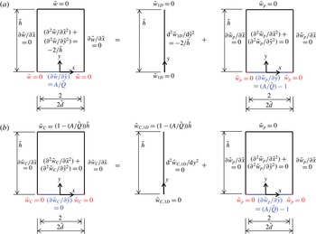
Utilizing superposition, we separate
 $\tilde{w}$
into one-dimensional (
 $\tilde{w}_{1D}$
) and perturbation (
 $\tilde{w}_{p}$
) components as per figure 2(a). It follows that
 $\tilde{w}_{1D}={\tilde{y}}-{\tilde{y}}^{2}/\tilde{h}$
and
 $\text{d}\tilde{w}_{1D}/\text{d}{\tilde{y}}|_{{\tilde{y}}=0}=1$
; therefore, the sum of the shear stresses imposed at the meniscus by the one-dimensional and perturbation problems equals that in the overall problem, i.e.
 $A/\tilde{Q}$
. Following Philip (Reference Philip1972a
), who considered the problem addressed here in the case of a shear-free meniscus, we embed the perturbation problem in an auxiliary Couette flow problem (
 $\tilde{w}_{C}$
) as per figure 2(b). Philip (Reference Philip1972a
) solved a problem of the same form as that for
 $\tilde{w}_{C}$
utilizing a conformal map. It follows from his solution that
 $$\begin{eqnarray}\tilde{w}_{p}=\text{Im}\left\{\frac{\left(1-{\displaystyle \frac{A}{\tilde{Q}}}\right)\tilde{h}}{K^{\prime }(k_{1})}\text{cn}^{-1}\left\{\frac{\text{cn}[\tilde{d}^{-1}K(k)(\tilde{x}+\text{i}{\tilde{y}}),k]}{\text{cn}[\tilde{d}^{-1}K(k),k]},k_{1}\right\}\right\}-\left(1-\frac{A}{\tilde{Q}}\right){\tilde{y}},\end{eqnarray}$$
where
 $k$
(not to be confused with the thermal conductivity of the liquid) and
 $k_{1}$
are such that
 $$\begin{eqnarray}\displaystyle & \displaystyle \frac{K^{\prime }(k)}{K(k)}=\tilde{h}/\tilde{d}, & \displaystyle\end{eqnarray}$$
 $$\begin{eqnarray}\displaystyle & \displaystyle k_{1}=k\,\text{cd}(\tilde{d}^{-1}K(k),k). & \displaystyle\end{eqnarray}$$
Modular notation has been used for the complete elliptic integral
 $K$
and its complement
 $K^{\prime }$
and for the Jacobi elliptic functions cn and cd and inverse function cn
 $^{-1}$
. The conformal map reduces the width of the domain from
 $2\tilde{d}$
to
 $2\tilde{d_{1}}$
, where
 $\tilde{d_{1}}$
, a parameter utilized below, is
 $$\begin{eqnarray}\tilde{d}_{1}=K(k_{1})\tilde{h}/K^{\prime }(k_{1}).\end{eqnarray}$$
(a) Dimensionless formulation of the problem in the Stokes flow limit and its one-dimensional and perturbation components. (b) Auxiliary Couette flow problem.

The shear-free boundary condition along the meniscus in the auxiliary Couette flow problem reduces the magnitude of the shear force required to move the liquid at the prescribed constant velocity at
 ${\tilde{y}}=\tilde{h}$
relative to the one-dimensional problem. Hence, the shear force exerted on the liquid in the perturbation component of this problem at
 ${\tilde{y}}=\tilde{h}$
is in the negative
 $z$
direction when
 $A/\tilde{Q}<1$
. Moreover, as discussed by Philip (Reference Philip1972b
), it is independent of
 ${\tilde{y}}$
because, for fully developed flow, the net shear force on any rectangular control volume spanning the width of the domain is zero. This implies that the mean velocity over the width of the domain
 $(\bar{\tilde{w}}_{p})$
varies linearly in
 ${\tilde{y}}$
(Philip Reference Philip1972b
). Again based upon a result of Philip (Reference Philip1972b
), it follows that
 $$\begin{eqnarray}\bar{\tilde{w}}_{p}=(1-A/\tilde{Q})(\tilde{h}-{\tilde{y}})(1-\tilde{d}_{1}/\tilde{d}).\end{eqnarray}$$
The dimensionless volumetric flow rate is
 $$\begin{eqnarray}\tilde{Q}=\int _{0}^{\tilde{h}}\bar{\tilde{w}}\tilde{d}\,\text{d}{\tilde{y}}.\end{eqnarray}$$
Performing the integration yields
 $$\begin{eqnarray}\tilde{Q}=\left[\frac{1}{6}+\frac{1-A/\tilde{Q}}{2}\left(1-\frac{\tilde{d}_{1}}{\tilde{d}}\right)\right]\tilde{h}^{2}\tilde{d},\end{eqnarray}$$
where the first and second terms in the brackets account for the one-dimensional and perturbative components of the solution respectively. Solution of this quadratic equation yields two solutions for
 $\tilde{Q}$
as per
 $$\begin{eqnarray}\tilde{Q}=\left({\textstyle \frac{1}{3}}\tilde{d}-{\textstyle \frac{1}{4}}\tilde{d}_{1}\right)\tilde{h}^{2}\pm \sqrt{\left({\textstyle \frac{1}{3}}\tilde{d}-{\textstyle \frac{1}{4}}\tilde{d}_{1}\right)^{2}\tilde{h}^{4}+{\textstyle \frac{1}{2}}A\tilde{h}^{2}(\tilde{d}_{1}-\tilde{d})}.\end{eqnarray}$$
Subjecting the one-dimensional form of (3.8) governing the mean streamwise velocity profile to the dimensionless Navier slip boundary condition, i.e.
 $\bar{\tilde{w}}=\tilde{b}(\text{d}\bar{\tilde{w}}/\text{d}{\tilde{y}})$
, at
 ${\tilde{y}}=0$
and the no-slip condition at
 ${\tilde{y}}=\tilde{h}$
yields
 $$\begin{eqnarray}\bar{\tilde{w}}=-\frac{{\tilde{y}}^{2}}{\tilde{h}}+\frac{\tilde{h}{\tilde{y}}+\tilde{h}\tilde{b}}{\tilde{h}+\tilde{b}}.\end{eqnarray}$$
The corresponding dimensionless volumetric flow rate is
 $$\begin{eqnarray}\tilde{Q}=\left[-\frac{\tilde{h}^{2}}{3}+\frac{\tilde{h}^{3}+2\tilde{b}\tilde{h}^{2}}{2(\tilde{h}+\tilde{b})}\right]\tilde{d}.\end{eqnarray}$$
Solving the preceding equation for the dimensionless slip length yields
 $$\begin{eqnarray}\frac{\tilde{b}}{\tilde{h}}=\frac{\tilde{d}\tilde{h}^{2}-6\tilde{Q}}{6\tilde{Q}-4\tilde{h}^{2}\tilde{d}}.\end{eqnarray}$$
Then, substituting the result for
 $\tilde{Q}$
from the conformal map solution as per (3.19) yields
 $$\begin{eqnarray}\frac{\tilde{b}}{\tilde{h}}=\frac{(\tilde{Q}-A)\left({\displaystyle \frac{\tilde{d}}{\tilde{d}_{1}}}-1\right)}{\tilde{Q}+A\left({\displaystyle \frac{\tilde{d}}{\tilde{d}_{1}}}-1\right)},\end{eqnarray}$$
where
 $\tilde{Q}$
is given by (3.20). In the absence of thermocapillary stress, (3.24) reduces to
 $$\begin{eqnarray}\frac{\tilde{b}}{\tilde{h}}=\frac{\tilde{d}}{\tilde{d}_{1}}-1.\end{eqnarray}$$
3.4 Asymptotic solution in the Stokes flow limit
The case when the channel height
 $h$
is sufficiently large in comparison with half of the pitch of the ridges,
 $d$
, can be accurately captured using a matched asymptotic expansion. If we denote the aspect ratio of the domain as
 $\unicode[STIX]{x1D716}=d/h$
, this corresponds to the limit
 $\unicode[STIX]{x1D716}\rightarrow 0$
, while keeping the cavity fraction (
 $\unicode[STIX]{x1D6FF}=a/d$
) fixed. Then, the flow field throughout the majority of the channel away from the wall structure (the ‘outer region’) turns out to be one-dimensional and parabolic, with exponentially small error, and the effect of the ridges is confined to a smaller region near
 $y=0$
where
 $y$
becomes comparable to the period of the ridges (the ‘inner region’, where
 $w=w(x,y)$
). This picture agrees well with many previous studies, but here we tackle it formally. The apparent slip due to the wall structure, seen by the one-dimensional outer flow, can then be found by matching the solutions in these two regions. We remark that the leading-order limit of large channel height compared with ridge period has been considered (without thermocapillary stress) by Teo & Khoo (Reference Teo and Khoo2009), but we present an alternative asymptotic method, and provide an exponentially accurate expression for the entire flow field, equation (3.58).
To improve the clarity of the derivation, and the picture of the different asymptotic regions in the domain, we introduce a different non-dimensionalization from that used in § 3.2. However, for the asymptotic results expressed in that non-dimensionalization scheme, see § 3.4.5. Here, we will instead normalize all lengths with respect to the largest length scale (for
 $\unicode[STIX]{x1D716}<1$
), the channel height
 $h$
, and consequently normalize the streamwise velocity with
 $(-\unicode[STIX]{x2202}p/\unicode[STIX]{x2202}z)h^{2}/(2\unicode[STIX]{x1D707})$
. The terms
 $A$
and
 $\tilde{Q}$
remain as defined in § 3.2. The non-dimensional streamwise-momentum equation becomes
 $$\begin{eqnarray}\frac{\unicode[STIX]{x2202}^{2}w}{\unicode[STIX]{x2202}x^{2}}+\frac{\unicode[STIX]{x2202}^{2}w}{\unicode[STIX]{x2202}y^{2}}=-2,\end{eqnarray}$$
where, for brevity, plain letters correspond to the new non-dimensional quantities. To make the rectangular domain independent of the asymptotic parameter, we rescale the
 $x$
variable to
 $X=x/\unicode[STIX]{x1D716}$
. The problem for
 $w(X,y)$
is then
 $$\begin{eqnarray}\displaystyle & \displaystyle \frac{1}{\unicode[STIX]{x1D716}^{2}}\frac{\unicode[STIX]{x2202}^{2}w}{\unicode[STIX]{x2202}X^{2}}+\frac{\unicode[STIX]{x2202}^{2}w}{\unicode[STIX]{x2202}y^{2}}=-2,\quad 0<X<1,0<y<1, & \displaystyle\end{eqnarray}$$
 $$\begin{eqnarray}\displaystyle & \displaystyle w=0,\quad 0<X<1,y=1, & \displaystyle\end{eqnarray}$$
 $$\begin{eqnarray}\displaystyle & \displaystyle \frac{\unicode[STIX]{x2202}w}{\unicode[STIX]{x2202}y}=\frac{A}{\tilde{Q}},\quad 0<X<\unicode[STIX]{x1D6FF},y=0, & \displaystyle\end{eqnarray}$$
 $$\begin{eqnarray}\displaystyle & \displaystyle w=0,\quad \unicode[STIX]{x1D6FF}<X<1,y=0, & \displaystyle\end{eqnarray}$$
with symmetry conditions
 $\unicode[STIX]{x2202}w/\unicode[STIX]{x2202}X=0$
on
 $X=0,\,1$
.
3.4.1 Outer region
In the limit of small
 $\unicode[STIX]{x1D716}$
, if we fix our position in the channel, this corresponds to keeping
 $X,y=O(1)$
as
 $\unicode[STIX]{x1D716}\rightarrow 0$
. This is the outer region. We expect the effect of the mixed boundary condition to vanish and
 $w$
to become independent of
 $X$
. As
 $\unicode[STIX]{x1D716}\rightarrow 0$
in (3.27) to leading order, we find
 $\unicode[STIX]{x2202}^{2}w/\unicode[STIX]{x2202}X^{2}=0$
, which, when integrated once and subjected to
 $\unicode[STIX]{x2202}_{X}w(0,y)=\unicode[STIX]{x2202}_{X}w(1,y)=0$
and then integrated again, implies that
 $w$
is purely a function of
 $y$
at leading order. Then, the remaining terms in (3.27) balance, giving the estimate
 $w=O(1)$
in the outer region. Therefore, we propose a formal asymptotic expansion
 $$\begin{eqnarray}w\sim w_{0}+\unicode[STIX]{x1D716}w_{1}+\unicode[STIX]{x1D716}^{2}w_{2}+\cdots =\mathop{\sum }_{n=0}^{\infty }\unicode[STIX]{x1D716}^{n}w_{n}(X,y),\quad \unicode[STIX]{x1D716}\rightarrow 0,\end{eqnarray}$$
where
 $w_{n}=O(1)$
for all
 $n\geqslant 0$
. Even though only
 $\unicode[STIX]{x1D716}^{2}$
appears in the problem (3.27)–(3.30), we expand in powers of
 $\unicode[STIX]{x1D716}$
, which will be necessary for matching with the inner solution near
 $y=0$
. Substituting (3.31) into (3.27), we find at each order in
 $\unicode[STIX]{x1D716}$
 $$\begin{eqnarray}\displaystyle & \displaystyle O(\unicode[STIX]{x1D716}^{-2}):\frac{\unicode[STIX]{x2202}^{2}w_{0}}{\unicode[STIX]{x2202}X^{2}}=0, & \displaystyle\end{eqnarray}$$
 $$\begin{eqnarray}\displaystyle & \displaystyle O(\unicode[STIX]{x1D716}^{-1}):\frac{\unicode[STIX]{x2202}^{2}w_{1}}{\unicode[STIX]{x2202}X^{2}}=0, & \displaystyle\end{eqnarray}$$
 $$\begin{eqnarray}\displaystyle & \displaystyle O(\unicode[STIX]{x1D716}^{0}):\frac{\unicode[STIX]{x2202}^{2}w_{2}}{\unicode[STIX]{x2202}X^{2}}+\frac{\unicode[STIX]{x2202}^{2}w_{0}}{\unicode[STIX]{x2202}y^{2}}=-2, & \displaystyle\end{eqnarray}$$
 $$\begin{eqnarray}\displaystyle & \displaystyle O(\unicode[STIX]{x1D716}^{n}):\frac{\unicode[STIX]{x2202}^{2}w_{n+2}}{\unicode[STIX]{x2202}X^{2}}+\frac{\unicode[STIX]{x2202}^{2}w_{n}}{\unicode[STIX]{x2202}y^{2}}=0,\quad n\geqslant 1. & \displaystyle\end{eqnarray}$$
The symmetry conditions
 $\unicode[STIX]{x2202}_{X}w_{n}(0,y)=\unicode[STIX]{x2202}_{X}w_{n}(1,y)=0$
apply at all orders. Integration of (3.33) along with the symmetry boundary conditions shows that
 $w_{1}$
is a function of
 $y$
only. Equation (3.34) and symmetry boundary conditions then imply that
 $\unicode[STIX]{x2202}^{2}w_{2}/\unicode[STIX]{x2202}X^{2}$
is a function of
 $y$
. By induction in
 $n$
, the remaining equations give
 $w_{n}=w_{n}(y)$
for all
 $n\geqslant 0$
. This means that
 $w$
is independent of
 $X$
at all orders in the
 $\unicode[STIX]{x1D716}$
expansion. The equations then collapse to
 $$\begin{eqnarray}\displaystyle & \displaystyle \frac{\text{d}^{2}w_{0}}{\text{d}y^{2}}=-2, & \displaystyle\end{eqnarray}$$
 $$\begin{eqnarray}\displaystyle & \displaystyle \frac{\text{d}^{2}w_{n}}{\text{d}y^{2}}=0,\quad n\geqslant 1. & \displaystyle\end{eqnarray}$$
Integrating and applying the no-slip conditions
 $w_{n}(1)=0,\,n\geqslant 0$
,
 $$\begin{eqnarray}\displaystyle & \displaystyle w_{0}(y)=-y^{2}+y+C_{0}(1-y), & \displaystyle\end{eqnarray}$$
 $$\begin{eqnarray}\displaystyle & \displaystyle w_{n}(y)=C_{n}(1-y),\quad n\geqslant 1, & \displaystyle\end{eqnarray}$$
where the
 $C_{n}$
are constants. The series (3.31) can then be written as
 $$\begin{eqnarray}w\sim -y^{2}+y+C(\unicode[STIX]{x1D716})(1-y),\end{eqnarray}$$
with
 $$\begin{eqnarray}C(\unicode[STIX]{x1D716}):=\mathop{\sum }_{n=0}^{\infty }C_{n}\unicode[STIX]{x1D716}^{n}.\end{eqnarray}$$
The mixed boundary conditions at
 $y=0$
cannot be satisfied by (3.40) since it has no
 $X$
dependence, so a different solution is needed near
 $y=0$
.
3.4.2 Inner region
We expect the effects of the ridges to become significant when
 $y$
is on the same scale as the pitch of the ridges, that is, when
 $y\sim x=O(\unicode[STIX]{x1D716})$
. This can be seen as the region where the
 $x$
and
 $y$
derivatives balance in the Laplacian of the governing equation,
 $\unicode[STIX]{x2202}^{2}/\unicode[STIX]{x2202}x^{2}\sim \unicode[STIX]{x2202}^{2}/\unicode[STIX]{x2202}y^{2}$
. Thus, we introduce inner variables
 $X=x/\unicode[STIX]{x1D716}$
and
 $Y=y/\unicode[STIX]{x1D716}$
, which we fix at
 $O(1)$
as
 $\unicode[STIX]{x1D716}\rightarrow 0.$
The scaling for
 $w$
here can be found from the behaviour of the outer solution as
 $y$
is decreased to
 $O(\unicode[STIX]{x1D716})$
. Substituting
 $y=\unicode[STIX]{x1D716}Y$
into (3.40),
 $$\begin{eqnarray}w\sim -\unicode[STIX]{x1D716}^{2}Y^{2}+\unicode[STIX]{x1D716}Y+C(\unicode[STIX]{x1D716})(1-\unicode[STIX]{x1D716}Y)\end{eqnarray}$$
or
 $$\begin{eqnarray}w\sim C_{0}+\unicode[STIX]{x1D716}[(1-C_{0})Y+C_{1}]+O(\unicode[STIX]{x1D716}^{2}).\end{eqnarray}$$
If
 $C(\unicode[STIX]{x1D716})=O(1)$
, i.e.
 $C_{0}\neq 0$
, then this implies
 $w=O(1)$
in the inner region (
 $Y=O(1)$
). Writing
 $w=W(X,Y)$
in this region, the problem for
 $W$
is
 $$\begin{eqnarray}\displaystyle & \displaystyle \frac{\unicode[STIX]{x2202}^{2}W}{\unicode[STIX]{x2202}X^{2}}+\frac{\unicode[STIX]{x2202}^{2}W}{\unicode[STIX]{x2202}Y^{2}}=-2\unicode[STIX]{x1D716}^{2},\quad 0<X<1,0<Y, & \displaystyle\end{eqnarray}$$
 $$\begin{eqnarray}\displaystyle & \displaystyle \frac{\unicode[STIX]{x2202}W}{\unicode[STIX]{x2202}Y}=\unicode[STIX]{x1D716}\frac{A}{\tilde{Q}},\quad 0<X<\unicode[STIX]{x1D6FF},Y=0, & \displaystyle\end{eqnarray}$$
 $$\begin{eqnarray}\displaystyle & \displaystyle W=0,\quad \unicode[STIX]{x1D6FF}<X<1,Y=0, & \displaystyle\end{eqnarray}$$
with symmetry conditions
 $\unicode[STIX]{x2202}_{X}W(0,Y)=\unicode[STIX]{x2202}_{X}W(1,Y)=0$
. The final condition on
 $W$
comes from the matching condition, which states that the outer expansion (
 $\unicode[STIX]{x1D716}\ll y<1$
) and the inner expansion (
 $0<y\ll 1$
) coincide in their overlap region,
 $\unicode[STIX]{x1D716}\ll y\ll 1$
(or
 $1\ll Y\ll \unicode[STIX]{x1D716}^{-1}$
). The outer solution in this overlap is given by (3.42), and the Van Dyke matching condition is that
 $$\begin{eqnarray}W\sim -\unicode[STIX]{x1D716}^{2}Y^{2}+\unicode[STIX]{x1D716}Y+C(\unicode[STIX]{x1D716})(1-\unicode[STIX]{x1D716}Y),\quad Y\rightarrow \infty .\end{eqnarray}$$
We can solve for
 $W$
by expansion,
 $$\begin{eqnarray}W\sim W_{0}+\unicode[STIX]{x1D716}W_{1}+\unicode[STIX]{x1D716}^{2}W_{2}+\cdots =\mathop{\sum }_{n=0}^{\infty }\unicode[STIX]{x1D716}^{n}W_{n},\quad \unicode[STIX]{x1D716}\rightarrow 0.\end{eqnarray}$$
Doing so, we find that the
 $O(1)$
problem for
 $W_{0}$
only permits the solution
 $W_{0}\equiv 0$
(as there is no shear rate at that order) and consequently
 $C_{0}=0$
. However, notice we can, in fact, solve the inner problem for
 $W$
exactly from (3.44)–(3.47). Writing
 $$\begin{eqnarray}W=-\unicode[STIX]{x1D716}^{2}Y^{2}+\unicode[STIX]{x1D716}\frac{A}{\tilde{Q}}Y+\unicode[STIX]{x1D716}\left[\left[1-C(\unicode[STIX]{x1D716})\right]-\frac{A}{\tilde{Q}}\right]\widehat{W},\end{eqnarray}$$
then, if
 $\widehat{W}$
satisfies
 $$\begin{eqnarray}\displaystyle & \displaystyle \frac{\unicode[STIX]{x2202}^{2}\widehat{W}}{\unicode[STIX]{x2202}X^{2}}+\frac{\unicode[STIX]{x2202}^{2}\widehat{W}}{\unicode[STIX]{x2202}Y^{2}}=0,\quad 0<X<1,0<Y, & \displaystyle\end{eqnarray}$$
 $$\begin{eqnarray}\displaystyle & \displaystyle \frac{\unicode[STIX]{x2202}\widehat{W}}{\unicode[STIX]{x2202}Y}=0,\quad 0<X<\unicode[STIX]{x1D6FF},Y=0, & \displaystyle\end{eqnarray}$$
 $$\begin{eqnarray}\displaystyle & \displaystyle \widehat{W}=0,\quad \unicode[STIX]{x1D6FF}<X<1,Y=0, & \displaystyle\end{eqnarray}$$
 $$\begin{eqnarray}\displaystyle & \displaystyle \widehat{W}\sim Y+\frac{C(\unicode[STIX]{x1D716})}{\unicode[STIX]{x1D716}[[1-C(\unicode[STIX]{x1D716})]-A/\tilde{Q}]},\quad Y\rightarrow \infty , & \displaystyle\end{eqnarray}$$
with symmetry conditions
 $\unicode[STIX]{x2202}_{X}\widehat{W}(0,Y)=\unicode[STIX]{x2202}_{X}\widehat{W}(1,Y)=0$
,
 $W$
will satisfy (3.44)–(3.46). This problem for
 $\widehat{W}$
has the solution (Philip Reference Philip1972a
)
 $$\begin{eqnarray}\displaystyle \left.\begin{array}{@{}rcl@{}}\widehat{W} & = & \text{Im}\left\{{\displaystyle \frac{2}{\unicode[STIX]{x03C0}}}\cos ^{-1}\left[{\displaystyle \frac{\cos (\unicode[STIX]{x03C0}Z/2)}{\cos (\unicode[STIX]{x1D6FF}\unicode[STIX]{x03C0}/2)}}\right]\right\}\\ & {\sim} & Y+F,\quad Y\rightarrow \infty ,\end{array}\right\} & & \displaystyle\end{eqnarray}$$
where
 $Z=X+\text{i}Y$
and
 $F=(2/\unicode[STIX]{x03C0})\log [\sec (\unicode[STIX]{x1D6FF}\unicode[STIX]{x03C0}/2)]$
. This determines
 $C(\unicode[STIX]{x1D716})$
to be
 $$\begin{eqnarray}C(\unicode[STIX]{x1D716})=\frac{(1-A/\tilde{Q})\unicode[STIX]{x1D716}F}{1+\unicode[STIX]{x1D716}F}\end{eqnarray}$$
and the inner solution (3.49) to be
 $$\begin{eqnarray}W\sim -\unicode[STIX]{x1D716}^{2}Y^{2}+\unicode[STIX]{x1D716}\frac{A}{\tilde{Q}}Y+\unicode[STIX]{x1D716}\left(\frac{1-A/\tilde{Q}}{1+\unicode[STIX]{x1D716}F}\right)\text{Im}\left\{\frac{2}{\unicode[STIX]{x03C0}}\cos ^{-1}\left[\frac{\cos (\unicode[STIX]{x03C0}Z/2)}{\cos (\unicode[STIX]{x1D6FF}\unicode[STIX]{x03C0}/2)}\right]\right\}.\end{eqnarray}$$
3.4.3 Composite solution
Since the outer (
 $\unicode[STIX]{x1D716}\ll y\leqslant 1$
) and inner (
 $0\leqslant Y\ll \unicode[STIX]{x1D716}^{-1}$
) expansions agree in the overlap region,
 $\unicode[STIX]{x1D716}\ll y\ll 1$
, a composite asymptotic solution uniformly valid in
 $y$
can be constructed as
 $$\begin{eqnarray}\displaystyle w_{comp}=w_{outer}+w_{inner}-w_{overlap}. & & \displaystyle\end{eqnarray}$$
However, the outer expansion keeps its form all the way into the overlap region (see (3.40) and (3.42)), so
 $w_{overlap}=w_{outer}$
, and their contributions cancel to give
 $$\begin{eqnarray}w_{comp}=w_{inner}.\end{eqnarray}$$
Therefore, the inner solution alone, given above by (3.56), is not only asymptotically correct to all orders in
 $\unicode[STIX]{x1D716}$
, but is uniformly valid throughout the entire domain, for any value of
 $A/\tilde{Q}$
.
3.4.4 Slip length
The slip length, denoted by
 $\unicode[STIX]{x1D6FD}$
rather than
 $b$
to distinguish the asymptotic and exact results for it, is found by equating the average velocity with that of a Navier slip profile of the form
 $$\begin{eqnarray}w=-y^{2}+\frac{y+\unicode[STIX]{x1D6FD}}{1+\unicode[STIX]{x1D6FD}},\end{eqnarray}$$
with slip length
 $\unicode[STIX]{x1D6FD}$
at
 $y=0$
. The average velocity of the asymptotic solution is calculated by splitting the domain at
 $y=\unicode[STIX]{x1D702}(\unicode[STIX]{x1D716})$
, in the overlap region,
 $$\begin{eqnarray}\displaystyle \bar{w} & = & \displaystyle \int _{0}^{1}\int _{0}^{1}w(X,y)\,\text{d}y\,\text{d}X\nonumber\\ \displaystyle & = & \displaystyle \int _{0}^{\unicode[STIX]{x1D702}(\unicode[STIX]{x1D716})}\left(\int _{0}^{1}w_{inner}\,\text{d}X\right)\text{d}y+\int _{\unicode[STIX]{x1D702}(\unicode[STIX]{x1D716})}^{1}\left(\int _{0}^{1}w_{outer}\text{d}X\right)\,\text{d}y,\quad \text{where }\unicode[STIX]{x1D716}\ll \unicode[STIX]{x1D702}(\unicode[STIX]{x1D716})\ll 1,\nonumber\\ \displaystyle & & \displaystyle\end{eqnarray}$$
where
 $w_{inner}$
and
 $w_{outer}$
are given by (3.40) and (3.49) respectively. However, it can be shown that
 $\int _{0}^{1}w_{inner}\text{d}X=\int _{0}^{1}w_{outer}\text{d}X=w_{outer}$
, using similar arguments to those in Philip (Reference Philip1972b
). Therefore,
 $\bar{w}$
can be calculated purely from the outer solution integrated down to
 $y=0$
,
 $$\begin{eqnarray}\bar{w}=\int _{0}^{1}w_{outer}\text{d}y=\frac{1}{6}+\frac{1}{2}C(\unicode[STIX]{x1D716}),\end{eqnarray}$$
giving a slip length
 $$\begin{eqnarray}\unicode[STIX]{x1D6FD}=\frac{(1-A/\tilde{Q})\unicode[STIX]{x1D716}F}{1+(A/\tilde{Q})\unicode[STIX]{x1D716}F}.\end{eqnarray}$$
The outer solution, written in terms of
 $\unicode[STIX]{x1D6FD}$
, is exactly the Navier slip profile (3.59). The quantity
 $\tilde{Q}$
can then be determined by enforcing
 $\tilde{Q}=\tilde{d}\tilde{h}^{2}\bar{w}$
, i.e.
 $$\begin{eqnarray}\tilde{Q}=\tilde{d}\tilde{h}^{2}\left[\frac{1}{6}+\frac{1}{2}\left(\frac{1-A/\tilde{Q}}{1+\unicode[STIX]{x1D716}F}\right)\unicode[STIX]{x1D716}F\right],\end{eqnarray}$$
resulting in a quadratic equation for
 $\tilde{Q}$
, just as in § 3.2.
3.4.5 Comparison with the exact solution
To compare the asymptotic solution with the exact conformal map solution (3.13), we rewrite the expressions (3.40), (3.56) and (3.61) using the original non-dimensional scheme described in § 3.2, and the transformation is given by
 $$\begin{eqnarray}\left.\begin{array}{@{}c@{}}w={\displaystyle \frac{1}{\tilde{h}}}\tilde{w},\quad W={\displaystyle \frac{1}{\tilde{h}}}\tilde{w},\\ x={\displaystyle \frac{1}{\tilde{h}}}\tilde{x},\quad X={\displaystyle \frac{1}{\tilde{d}}}\tilde{x},\\ y={\displaystyle \frac{1}{\tilde{h}}}{\tilde{y}},\quad Y={\displaystyle \frac{1}{\tilde{d}}}{\tilde{y}},\\ \unicode[STIX]{x1D6FD}={\displaystyle \frac{1}{\tilde{h}}}\tilde{\unicode[STIX]{x1D6FD}},\quad \unicode[STIX]{x1D716}={\displaystyle \frac{\tilde{d}}{\tilde{h}}}.\end{array}\right\}\end{eqnarray}$$
First, note that the limit
 $\unicode[STIX]{x1D716}=d/h\rightarrow 0$
with
 $a/d$
fixed (which we have assumed here) is equivalent to
 $\tilde{h}\rightarrow \infty$
with
 $\tilde{d}$
fixed. In the outer region, where now we have
 ${\tilde{y}}=O(\tilde{h})$
as
 $\tilde{h}\rightarrow \infty$
, we have a Navier slip profile,
 $$\begin{eqnarray}\tilde{w}_{outer}\sim -\frac{{\tilde{y}}^{2}}{\tilde{h}}+\frac{\tilde{h}({\tilde{y}}+\tilde{\unicode[STIX]{x1D6FD}})}{\tilde{h}+\tilde{\unicode[STIX]{x1D6FD}}}.\end{eqnarray}$$
The inner region is now
 ${\tilde{y}}=O(1)$
, in which we have
 $$\begin{eqnarray}\tilde{w}_{inner}\sim -\frac{{\tilde{y}}^{2}}{\tilde{h}}+\frac{A}{\tilde{Q}}\,{\tilde{y}}+\tilde{d}\left(\frac{1-A/\tilde{Q}}{1+\unicode[STIX]{x1D716}F}\right)\text{Im}\left(\frac{2}{\unicode[STIX]{x03C0}}\cos ^{-1}\left\{\frac{\cos [\unicode[STIX]{x03C0}(\tilde{x}+\text{i}{\tilde{y}})/(2\tilde{d})]}{\cos [\unicode[STIX]{x03C0}/(2\tilde{d})]}\right\}\right),\end{eqnarray}$$
with
 $$\begin{eqnarray}F=\frac{2}{\unicode[STIX]{x03C0}}\log \left[\sec \left(\frac{\unicode[STIX]{x03C0}}{2\tilde{d}}\right)\right].\end{eqnarray}$$
The slip length is given by
 $$\begin{eqnarray}\frac{\tilde{b}}{\tilde{h}}\sim \frac{\tilde{\unicode[STIX]{x1D6FD}}}{\tilde{h}}=\frac{(\tilde{Q}-A)\unicode[STIX]{x1D716}F}{\tilde{Q}+A\unicode[STIX]{x1D716}F}=\frac{\tilde{d}\tilde{h}^{2}-6\tilde{Q}}{6\tilde{Q}-4\tilde{h}^{2}\tilde{d}},\end{eqnarray}$$
and the two solutions from the quadratic equation (3.62) for
 $\tilde{Q}$
are given by
 $$\begin{eqnarray}\tilde{Q}=\tilde{d}\tilde{h}^{2}\frac{1+4\unicode[STIX]{x1D716}F\pm \sqrt{(1+4\unicode[STIX]{x1D716}F)^{2}-72\unicode[STIX]{x1D716}F(1+\unicode[STIX]{x1D716}F)A/(\tilde{d}\tilde{h}^{2})}}{12(1+\unicode[STIX]{x1D716}F)}.\end{eqnarray}$$
These are identical to the exact expressions for
 $\tilde{Q}$
and
 $\tilde{b}/\tilde{h}$
found from the conformal map, but with the quantity
 $\tilde{d}/\tilde{d}_{1}-1$
replaced everywhere with
 $\unicode[STIX]{x1D716}F$
. This can be explained by observing that
 $\tilde{d}/\tilde{d}_{1}-1$
is the exact slip length with no thermocapillary stress (
 $A/\tilde{Q}=0$
), and the asymptotic approximation in that case is
 $\unicode[STIX]{x1D716}F$
(from (3.67)). However,
 $\tilde{d}/\tilde{d}_{1}-1$
depends only on the geometry, and so the approximation
 $\tilde{d}/\tilde{d}_{1}-1\sim \unicode[STIX]{x1D716}F$
as
 $\unicode[STIX]{x1D716}\rightarrow 0$
should hold independent of thermocapillary stress.
All quantities, except
 $A$
, in the expressions for
 $\tilde{Q}$
given by (3.19) and (3.68) are positive. (The term
 $A$
is negative, 0 and positive when
 $q_{sl}^{\prime \prime }$
is positive, 0 and negative, i.e. heat is transferred from the liquid into the ridges respectively.) Hence, both of the roots for
 $\tilde{Q}$
are real provided that
 $$\begin{eqnarray}A\leqslant A_{max}=\frac{2\left(\frac{1}{3}\tilde{d}-\frac{1}{4}\tilde{d}_{1}\right)^{2}\tilde{h}^{2}}{\tilde{d}-\tilde{d}_{1}}\sim \frac{\tilde{d}\tilde{h}^{2}(1+4\unicode[STIX]{x1D716}F)^{2}}{72\unicode[STIX]{x1D716}F(1+\unicode[STIX]{x1D716}F)}.\end{eqnarray}$$
In the limit
 $A\rightarrow 0$
, the solution with the
 $(+)$
collapses to the unique non-trivial solution in the absence of thermocapillary stress. The
 $(-)$
solution tends to one with zero flow rate,
 $\tilde{Q}=0$
, but with non-zero thermocapillary stress,
 $A/\tilde{Q}=(4\tilde{d}/3-\tilde{d}_{1})/(\tilde{d}-\tilde{d}_{1})$
, its maximum value. Hence, we expect the
 $(+)$
solution to be more physically relevant. For the
 $(+)$
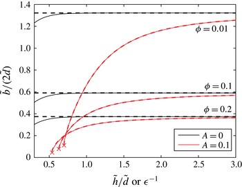
solution, figure 3 compares the asymptotic slip length with the exact slip length when thermocapillary stress is present
 $(A=0.1)$
and absent
 $(A=0)$
. The solutions agree extremely well for
 $A=0$
, even when
 $\unicode[STIX]{x1D716}=1$
, but there is even better agreement when
 $A\neq 0$
. The solutions are indistinguishable all the way down to the critical point where the solutions cease to exist, where
 $A=A_{max}$
. This allows one to use the simple logarithmic expression for
 $F$
instead of calculating
 $\tilde{d}_{1}$
from the cumbersome elliptic integral map, with very small error, even for square domains
 $\tilde{h}/\tilde{d}=1$
. Finally, we note that there is no restriction that
 $A\geqslant 0$
in the derived expressions. When
 $A<0$
because, for example, heat transfer is from the liquid into the ridges, there are always two real solutions and we still expect the
 $(+)$
solution to be more physically relevant since it collapses to the correct solution as
 $A\rightarrow 0$
.
Slip length
 $\tilde{b}/(2\tilde{d})$
with thermocapillary stress (red curves) and without it (black curves) for various solid fractions (
 $\unicode[STIX]{x1D719}$
). The solid curves are the exact solutions and the dashed curves are the asymptotic solutions for
 $\unicode[STIX]{x1D716}\rightarrow 0$
. Only the
 $(+)$
branch is shown. Crosses indicate when a solution ceases to exist.

3.4.6 Error quantification
Here, we utilize the exact solution to verify that the errors in the slip lengths and velocity field given by the asymptotic one are exponentially small in the
 $\unicode[STIX]{x1D716}\rightarrow 0$
limit. We recall that the parameters
 $k$
,
 $k_{1}$
and
 $d_{1}$
characterizing the conformal map used to find it are defined by (3.14), (3.15) and (3.16) respectively. In terms of
 $\unicode[STIX]{x1D716}$
, equation (3.14) becomes
 $$\begin{eqnarray}\frac{K^{\prime }(k)}{K(k)}=\frac{1}{\unicode[STIX]{x1D716}}.\end{eqnarray}$$
Additionally, by noting that
 $\text{cd}[K(k)/\tilde{d},k]=\text{cn}[K(k)/\tilde{d},k]/\text{dn}[K(k)/\tilde{d},k]$
and using relations 8.146(2) and 8.146(3) in Gradshteyn & Ryzhik (Reference Gradshteyn and Ryzhik2014) for the expansions of
 $\text{cn}$
and
 $\text{dn}$
in Lambert series in terms of the nome,
 $q=\text{exp}[-\unicode[STIX]{x03C0}K^{\prime }(k)/K(k)]$
, or, presently,
 $q=\exp (-\unicode[STIX]{x03C0}/\unicode[STIX]{x1D716})$
, it follows from (3.15) that
 $$\begin{eqnarray}k_{1}=\frac{\displaystyle \mathop{\sum }_{n=0}^{\infty }\frac{q^{n+1/2}}{1+q^{2n+1}}\cos \left[(2n+1)\frac{\unicode[STIX]{x03C0}}{2\tilde{d}}\right]}{{\displaystyle \frac{1}{4}}+\displaystyle \mathop{\sum }_{n=1}^{\infty }{\displaystyle \frac{q^{n}}{1+q^{2n}}}\cos \left[2n{\displaystyle \frac{\unicode[STIX]{x03C0}}{2\tilde{d}}}\right]}.\end{eqnarray}$$
Since
 $q$
is exponentially small in the limit as
 $\unicode[STIX]{x1D716}\rightarrow 0$
, it follows that
 $$\begin{eqnarray}k_{1}=4q^{1/2}\cos \left(\frac{\unicode[STIX]{x03C0}}{2\tilde{d}}\right)+O(q^{3/2}(\unicode[STIX]{x1D716})),\quad \unicode[STIX]{x1D716}\rightarrow 0.\end{eqnarray}$$
To evaluate
 $\tilde{d}_{1}$
when
 $\unicode[STIX]{x1D716}\rightarrow 0$
, we first express (3.16) as
 $$\begin{eqnarray}\frac{\tilde{d}}{\tilde{d}_{1}}=\unicode[STIX]{x1D716}\frac{K^{\prime }(k_{1})}{K(k)}.\end{eqnarray}$$
Noting that
 $k_{1}\rightarrow 0$
as
 $\unicode[STIX]{x1D716}\rightarrow 0$
, it follows from the series representations of the complete elliptic integral given by relations 8.113(1) and 8.113(3) in Gradshteyn & Ryzhik (Reference Gradshteyn and Ryzhik2014) that
 $$\begin{eqnarray}\displaystyle & \displaystyle K^{\prime }(k_{1})=-\log \left(\frac{k_{1}}{4}\right)+O(k_{1}^{2}\log k_{1}),\quad k_{1}\rightarrow 0, & \displaystyle\end{eqnarray}$$
 $$\begin{eqnarray}\displaystyle & \displaystyle K(k_{1})=\frac{\unicode[STIX]{x03C0}}{2}+O(k_{1}^{2}),\quad k_{1}\rightarrow 0. & \displaystyle\end{eqnarray}$$
Utilizing the foregoing expressions and (3.72), (3.73) becomes
 $$\begin{eqnarray}\displaystyle \frac{\tilde{d}}{\tilde{d}_{1}}=\frac{2}{\unicode[STIX]{x03C0}}\unicode[STIX]{x1D716}\left\{-\frac{1}{2}\log q+\log \left[\sec \left(\frac{\unicode[STIX]{x03C0}}{2\tilde{d}}\right)\right]+O(q\log q)\right\},\quad q\rightarrow 0, & & \displaystyle\end{eqnarray}$$
or, in terms of
 $\unicode[STIX]{x1D716}$
,
 $$\begin{eqnarray}\frac{\tilde{d}}{\tilde{d}_{1}}=1+\unicode[STIX]{x1D716}F+O(\text{e}^{-\unicode[STIX]{x03C0}/\unicode[STIX]{x1D716}}),\quad \unicode[STIX]{x1D716}\rightarrow 0.\end{eqnarray}$$
Substituting this result into (3.20), we find that
 $\tilde{Q}^{\pm }=\tilde{Q}_{asym}^{\pm }+O(\unicode[STIX]{x1D716}^{-2}\text{e}^{-\unicode[STIX]{x03C0}/\unicode[STIX]{x1D716}})$
, where the
 $\tilde{Q}_{asym}^{\pm }$
are the asymptotic solutions as per (3.68). It can further be shown that
 $\tilde{Q}_{asym}^{+}=O(1/\unicode[STIX]{x1D716}^{2})$
and
 $\tilde{Q}_{asym}^{-}=O(\unicode[STIX]{x1D716})$
, from which it follows that
 $$\begin{eqnarray}\displaystyle & \displaystyle \frac{\tilde{b}}{\tilde{h}}^{+}=\frac{\tilde{\unicode[STIX]{x1D6FD}}}{\tilde{h}}^{+}+O(\text{e}^{-\unicode[STIX]{x03C0}/\unicode[STIX]{x1D716}}), & \displaystyle\end{eqnarray}$$
 $$\begin{eqnarray}\displaystyle & \displaystyle \frac{\tilde{b}}{\tilde{h}}^{-}=\frac{\tilde{\unicode[STIX]{x1D6FD}}}{\tilde{h}}^{-}+O(\unicode[STIX]{x1D716}^{-5}\text{e}^{-\unicode[STIX]{x03C0}/\unicode[STIX]{x1D716}}). & \displaystyle\end{eqnarray}$$
Hence, the error in the slip lengths computed from the matched asymptotic expansion is confirmed to be exponentially small, but takes a different form depending upon the root chosen for
 $\tilde{Q}$
. Finally, it follows immediately that (3.78) also holds in the absence of thermocapillary stress (
 $A=0$
).
The behaviour of the exact solution for the velocity field given by (3.13) when
 $\unicode[STIX]{x1D716}\rightarrow 0$
follows from that of
 $\tilde{Q}$
provided above and that of the quantity
 $$\begin{eqnarray}\unicode[STIX]{x1D709}=\frac{\tilde{h}}{K^{\prime }(k_{1})}\text{cn}^{-1}\left\{\frac{\text{cn}[\tilde{d}^{-1}K(k)\tilde{z},k]}{\text{cn}[\tilde{d}^{-1}K(k),k]},k_{1}\right\},\quad \text{where }\tilde{z}=\tilde{x}+\text{i}{\tilde{y}}.\end{eqnarray}$$
Moreover, upon replacing
 $\tilde{h}/K^{\prime }(k)$
with
 $\tilde{d}_{1}/K(k)$
as per (3.16) and rearranging,
 $$\begin{eqnarray}\text{cn}[\tilde{d}_{1}^{-1}K(k_{1})\unicode[STIX]{x1D709},k_{1}]=\frac{\text{cn}[\tilde{d}^{-1}K(k)\tilde{z},k]}{\text{cn}[\tilde{d}^{-1}K(k),k]}.\end{eqnarray}$$
We note that from (3.73) the left-hand side of (3.76) is
 $\unicode[STIX]{x1D716}K^{\prime }(k_{1})/K(k_{1})$
, such that the nome of
 $k_{1}$
, which we denote by
 $q_{1}$
, becomes
 $q_{1}\sim \text{e}^{-\unicode[STIX]{x03C0}F}q+O(q^{2})$
. Then, using the previously mentioned expansion for cn in terms of the nome, the preceding equation becomes
 $$\begin{eqnarray}\frac{2\unicode[STIX]{x03C0}}{K(k_{1})\,k_{1}}\left[\text{e}^{-\unicode[STIX]{x03C0}F/2}q^{1/2}\cos \left(\frac{\unicode[STIX]{x03C0}}{2\tilde{d}_{1}}\unicode[STIX]{x1D709}\right)+O(q^{3/2})\right]=\frac{\cos \left({\displaystyle \frac{\unicode[STIX]{x03C0}}{2\tilde{d}}}\tilde{z}\right)}{\cos \left({\displaystyle \frac{\unicode[STIX]{x03C0}}{2\tilde{d}}}\right)}+O(q),\quad q\rightarrow 0.\end{eqnarray}$$
It then follows from (3.72), (3.75) and (3.77) that, after rearrangement,
 $$\begin{eqnarray}\unicode[STIX]{x1D709}=\frac{2}{\unicode[STIX]{x03C0}}\frac{\tilde{d}}{1+\unicode[STIX]{x1D716}F}\cos ^{-1}\left[\frac{\cos \left({\displaystyle \frac{\unicode[STIX]{x03C0}}{2\tilde{d}}}\tilde{z}\right)}{\cos \left({\displaystyle \frac{\unicode[STIX]{x03C0}}{2\tilde{d}}}\right)}\right]+O(q^{1/2}).\end{eqnarray}$$
The form of the exact solution (
 $\tilde{w}$
) in the
 $\unicode[STIX]{x1D716}\rightarrow 0$
limit follows by evaluating its perturbative component as per (3.13) and adding the one-dimensional component, i.e.
 $-{\tilde{y}}^{2}/\tilde{h}+{\tilde{y}}$
, to the result. Comparison with the composite matched asymptotic solution (
 $\tilde{w}_{comp}$
) shows that
 $$\begin{eqnarray}\tilde{w}=\tilde{w}_{comp}+O(\text{e}^{-\unicode[STIX]{x03C0}/\unicode[STIX]{x1D716}}),\quad \unicode[STIX]{x1D716}\rightarrow 0.\end{eqnarray}$$
We remark that this holds for both choices of sign in
 $\tilde{Q}$
, and at every fixed location
 $\tilde{z}=\tilde{x}+\text{i}{\tilde{y}}$
throughout the domain. Therefore, we have not only validated the matched asymptotics, but confirmed that the accuracy is to all orders in
 $\unicode[STIX]{x1D716}$
and provided the asymptotic error terms – see (3.78), (3.79) and (3.84).
3.5 Numerical solution to the general problem
The general problem is governed by the three-dimensional steady-state forms of the continuity, Navier–Stokes and thermal energy equations. It was solved using FLUENT® with the viscous dissipation terms in the thermal energy equation set equal to zero.
Given the symmetry of the problem with respect to the
 $y$
-axis, the computational domain corresponded only to the right half of the domain depicted in figure 1, i.e.
 $0<x<d$
and
 $0<y<h$
. Moreover, the computational domain necessarily had a finite streamwise length
 $\unicode[STIX]{x1D6FF}z$
due to the structure of FLUENT®. The boundary conditions at the solid–liquid interfaces, at the meniscus and at
 $x=d$
were the same as those described in § 2, and a mirror symmetry boundary condition was imposed at
 $x=0$
. Conditions of hydrodynamically and thermally developed flow were imposed by imposing a translational periodic boundary condition (Patankar, Liu & Sparrow Reference Patankar, Liu and Sparrow1977; ANSYS 2013) between the boundaries at
 $z=0$
and
 $z=\unicode[STIX]{x1D6FF}z$
. Thus, the pressure and temperature fields were separated into linear and periodic components, where the former come from the prescription of
 $(-\unicode[STIX]{x2202}p/\unicode[STIX]{x2202}z)$
and that of
 $q_{sl}^{\prime \prime }$
, along with (2.6). The periodic components of
 $p$
and
 $T$
vanish upon convergence.
The governing equations were discretized using a second-order upwind scheme and, because the velocity and temperature fields are coupled, they were simultaneously computed in an iterative manner. The steps of the solution process were as follows. At the
 $n$
th iteration, the thermocapillary stress along the meniscus was calculated utilizing the computed temperature field from the
 $(n-1)$
th iteration, and, subsequently, the continuity equation and the Navier–Stokes equations were solved using the pressure-based coupled solver. Next, the thermal energy equation was solved utilizing the new velocity field. These steps were repeated sequentially until convergence.
Mesh independence was achieved by adopting the following procedure. The domain was initially discretized with a uniform structured mesh, and the model was executed. Then, the mesh was refined utilizing the gradient and boundary adaptation options in FLUENT®, and the model was executed again. The mesh refinement procedure was repeated four or five times for each case. The calculated value of
 $\tilde{b}$
changed by less than 0.1 % after the final mesh refinement. Given that the mesh refinement was case-dependent, the final number of control volumes for each case was different, but it was always greater than 6.1 million.
4 Illustrative results
4.1 Analytical
There is a single value of the dimensionless parameter
 $A$
for a prescribed set of physical parameters, but the analytical solutions show that there are two real solutions for
 $\tilde{Q}$
(and
 $\tilde{b}$
) when
 $A<A_{max}$
, one when
 $A=A_{max}$
, and none when
 $A>A_{max}$
, as per (3.20) and (3.68). Therefore, when
 $A>A_{max}$
, no steady-state fully developed solutions exist. This is consistent with our numerical model, which did not converge when
 $A>A_{max}$
. For the range
 $0<A<A_{max}$
, both solution branches,
 $(+)$
and
 $(-)$
, for the slip length
 $(\tilde{b}/(2\tilde{d}))$
and shear stress
 $(A/\tilde{Q})$
for selected solid fractions and
 $\tilde{h}/\tilde{d}=1$
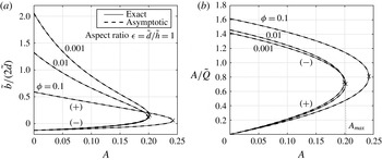
are shown in figure 4. The upper and lower branches for
 $\tilde{b}/(2\tilde{d})$
correspond to the
 $(+)$
and
 $(-)$
solutions respectively. The opposite is true for the shear stress,
 $A/\tilde{Q}$
. The crosses indicate the critical point, i.e. saddle-node bifurcation, at
 $A=A_{max}$
where the solution branches meet and annihilate, leaving no solutions for larger values of
 $A$
. Even though
 $\tilde{h}/\tilde{d}=1$
in figure 4, the asymptotic solution (dashed lines) is indistinguishable from the exact solution (solid lines) for all parameter values.
Both solution branches,
 $(+)$
and
 $(-)$
, of
 $(a)$
the dimensionless slip length and
 $(b)$
the dimensionless thermocapillary stress as
 $A$
is varied. Crosses indicate saddle-node bifurcations at
 $A=A_{max}$
. The aspect ratio
 $\tilde{h}/\tilde{d}=1$
, and
 $\unicode[STIX]{x1D719}$
values are labelled.

When the solutions exist, increasing
 $A$
increases the shear stress
 $A/\tilde{Q}$
for the
 $(+)$
branch, and decreases
 $A/\tilde{Q}$
for the
 $(-)$
branch, until
 $A/\tilde{Q}=1/2(4\tilde{d}/3-\tilde{d}_{1})/(\tilde{d}-\tilde{d}_{1})$
at the bifurcation point. Consequently, there is a decrease in slip for the
 $(+)$
branch and an increase in slip for the
 $(-)$
branch. Since the
 $(+)$
branch collapses to the classical solution in the absence of thermocapillary stress as
 $A\rightarrow 0$
, and behaves as we expect physically as
 $A$
is increased, it is most likely the stable solution realizable in experiments – at least for sufficiently small
 $A$
. Indeed, the numerical schemes employed in § 3.5 found only the
 $(+)$
branch. The
 $(-)$
branch is likely to be temporally unstable, but such a determination would need full time-dependent simulations of the coupled hydrodynamic and thermal problems.
Lastly, results are presented for two liquids, water and Galinstan, a liquid metal. Galinstan is relevant because structured surfaces may be used to enhance its effectiveness as a coolant in the thermal management of electronics, as discussed by Lam et al. (Reference Lam, Hodes and Enright2015). We set
 $d=10\,\unicode[STIX]{x03BC}\text{m}$
and
 $\tilde{h}/\tilde{d}=2$
and consider solid fractions in the range
 $0.001\leqslant \unicode[STIX]{x1D719}\leqslant 1$
for illustrative purposes. The pressure gradient used is the maximum value,
 $\unicode[STIX]{x2202}p/\unicode[STIX]{x2202}z|_{max}$
, such that the liquid remains in the Cassie state at the inlet to a 1 cm long channel, where the pressure difference across the meniscus is highest. This pressure difference is supported by the upward surface tension forces along the triple contact lines, and as per Lam et al. (Reference Lam, Hodes and Enright2015) it follows that
 $$\begin{eqnarray}\left.\frac{\unicode[STIX]{x2202}p}{\unicode[STIX]{x2202}z}\right|_{max}=\frac{\unicode[STIX]{x1D70E}\cos (\unicode[STIX]{x03C0}-\unicode[STIX]{x1D703}_{A})}{\text{d}L},\end{eqnarray}$$
where
 $\unicode[STIX]{x1D703}_{A}$
is the advancing contact angle and
 $L$
is the channel length. The parameter
 $A$
is expressed as
 $$\begin{eqnarray}A=\overbrace{\frac{-4(\text{d}\unicode[STIX]{x1D70E}/\text{d}T)q_{sl}^{\prime \prime }\unicode[STIX]{x1D707}L^{2}}{\unicode[STIX]{x1D70C}d^{2}c_{p}\unicode[STIX]{x1D70E}^{2}\cos ^{2}(\unicode[STIX]{x03C0}-\unicode[STIX]{x1D703}_{A})}}^{A^{\ast }}\frac{\unicode[STIX]{x1D719}}{(h/d)^{2}(1-\unicode[STIX]{x1D719})}.\end{eqnarray}$$
The parameter
 $A^{\ast }$
defined by the preceding equation depends on thermophysical and external parameters and the ridge pitch, but it is independent of the solid fraction
 $(\unicode[STIX]{x1D719})$
and aspect ratio
 $(h/d)$
. We prescribe a heat flux at the solid–liquid interface of
 $25~\text{W}~\text{cm}^{-2}$
and obtain the relevant thermophysical properties from those compiled by Lam et al. (Reference Lam, Hodes and Enright2015), except for the values of
 $(\text{d}\unicode[STIX]{x1D70E}/\text{d}T)$
, which follow from Lemmon, McLinden & Friend (Reference Lemmon, McLinden, Friend, Linstrom and Mallard2015) for water and, albeit not to a great degree of accuracy, from Prokhorenko et al. (Reference Prokhorenko, Roshchupkin, Pokrasin, Prokhorenko and Kotov2000) for Galinstan. It follows that
 $A^{\ast }=58.0$
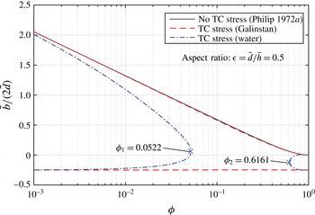
in the case of water and 0.797 in the case of Galinstan. Figure 5 shows the slip length against
 $\unicode[STIX]{x1D719}$
with
 $A^{\ast }$
fixed at zero (thermocapillary stress neglected) and its value for each liquid. Both solution branches are shown in the latter cases only for illustrative purposes. The effect of thermocapillary stress is very small for Galinstan as the
 $(+)$
branch is only slightly lower than if it was neglected. However, thermocapillary stress, except at sufficiently low or high solid fractions, substantially reduces the slip length in the case of water, e.g. from 0.795 to 0.0591 at a solid fraction of 0.0522. Moreover, because of the distinct functional dependences of
 $A_{max}$
and
 $A$
on the solid fraction, steady-state solutions exist only for
 $\unicode[STIX]{x1D719}\leqslant 0.0522$
or
 $\unicode[STIX]{x1D719}\geqslant 0.6161$
.
Dimensionless slip length versus solid fraction when thermocapillary (TC) stress is included for water (
 $A^{\ast }=58.0$
) and Galinstan (
 $A^{\ast }=0.797$
), compared with when it is neglected (
 $A^{\ast }=0$
).

4.2 Numerical
We performed numerical simulations for a domain with an aspect ratio,
 $\tilde{h}/\tilde{d}$
, of 4 and solid fraction,
 $\unicode[STIX]{x1D719}$
, of 0.025, such that
 $|\tilde{x}|\leqslant 1.03$
and
 $0\leqslant {\tilde{y}}\leqslant 4.10$
. The Prandtl number of the liquid was 0.043, typical of a liquid metal such as Galinstan, and the dimensionless parameters
 $A$
and
 $Br$
were 1 and
 $7.87\times 10^{-7}$
respectively. By varying the quantity
 $\unicode[STIX]{x1D70C}(\text{d}\unicode[STIX]{x1D70E}/\text{d}T)$
while holding the ratio
 $(\text{d}\unicode[STIX]{x1D70E}/\text{d}T)/\unicode[STIX]{x1D70C}$
constant, five transverse Reynolds numbers, i.e.
 $\mathit{Re}_{\bot }=3.90\times 10^{-3},3.90\times 10^{-2},0.390,3.90$
and 39.0, were considered. (The corresponding Reynolds numbers based on the hydraulic diameter of the channel (
 $2h$
) are 3.08, 9.74, 30.8, 97.1 and 279.)
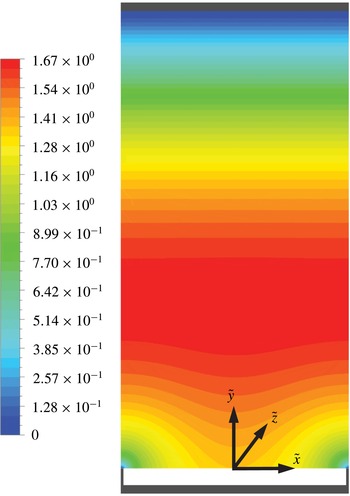
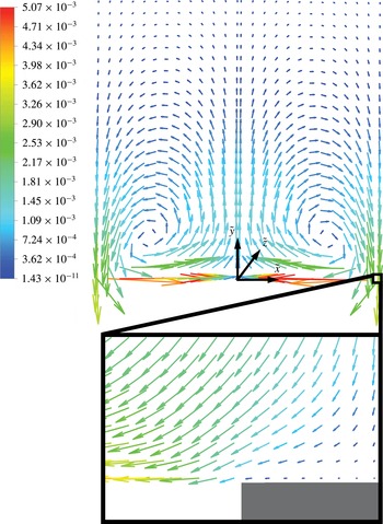
The computed three-dimensional velocity field when
 $\mathit{Re}_{\bot }=3.90\times 10^{-3}$
is presented in figure 6 (contour plot of dimensionless streamwise velocity field) and figure 7 (vector plot of dimensionless transverse velocity field). Velocities in both of these figures have been non-dimensionalized by
 $ah(-\unicode[STIX]{x2202}p/\unicode[STIX]{x2202}z)/(2\unicode[STIX]{x1D707})$
. Even the maximum transverse speed of the flow is more than an order of magnitude smaller than the characteristic streamwise one. Moreover, as expected, the flow field is close to unidirectional and one-dimensional one half of a dimensionless ridge pitch (
 $\tilde{d}$
) away from the composite interface. The transverse thermocapillary stress along the meniscus drives liquid from the triple contact lines towards the centre of the meniscus and produces a pair of counter-rotating vortices, as shown in figure 7.
Dimensionless streamwise velocity (
 $\tilde{w}$
) field when
 $\mathit{Re}_{\bot }=3.90\times 10^{-3}$
,
 $|\tilde{x}|\leqslant 1.03=\tilde{d}$
and
 $0\leqslant {\tilde{y}}\leqslant 4.10=\tilde{h}$
.

Dimensionless transverse velocity field when
 $\mathit{Re}_{\bot }=3.90\times 10^{-3}$
. The domain spans
 $|\tilde{x}|\leqslant 1.03=\tilde{d}$
and
 $0\leqslant {\tilde{y}}\leqslant 4.10=\tilde{h}$
. The regions shown correspond to
 $|\tilde{x}|\leqslant 1.03$
and
 $0\leqslant {\tilde{y}}\leqslant 2.05$
(upper figure) and
 $0.97\leqslant \tilde{x}\leqslant 1.03$
and
 $0\leqslant {\tilde{y}}\leqslant 0.03$
(lower figure). The tails of the velocity vectors in the upper figure are within the (liquid) domain, but some of their heads protrude out of it.

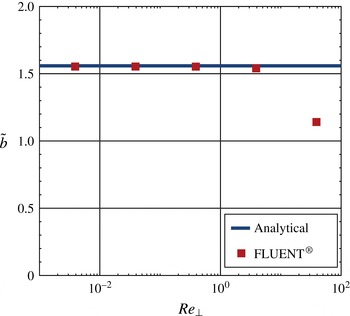
The numerically computed
 $\tilde{b}$
values are compared with the analytical results in figure 8. The corresponding discrepancies starting from the minimum value of
 $\mathit{Re}_{\bot }$
are 0.35 %, 0.35 %, 0.39 %, 1.21 % and 26.81 % respectively. As expected, at sufficiently high transverse Reynolds number, the analytical result for
 $\tilde{b}$
is invalid as it does not capture inertial effects, which reduce the slip length.
Plot of
 $\tilde{b}$
versus
 $\mathit{Re}_{\bot }$
, showing that the exact solution breaks down at sufficiently high
 $Re_{\bot }$
due to inertial effects.

5 Conclusions
We analytically and numerically computed the slip length for laminar Poiseuille flow in the Cassie state over uniform width and pitch parallel (streamwise) ridges on one side of a parallel-plate channel. Menisci between ridges were considered to be smooth and adiabatic. No-slip and constant heat flux boundary conditions were imposed at the solid–liquid interfaces between the ridge tips and liquid on the textured side of the channel. The opposite side was flat (no slip) and adiabatic. Streamwise thermocapillary stress along menisci was accounted for and could be set equal to zero to compute the slip length for an adiabatic flow. The functional dependence of the dimensionless slip length (
 $b/d$
) on the ridge solid fraction (
 $\unicode[STIX]{x1D719}$
), dimensionless channel height (
 $h/d$
) and a dimensionless parameter characterizing streamwise thermocapillary stress (
 $A$
) for the above flow configurations has been established. Our analytical results are valid provided that the transverse Reynolds number is small enough that the streamwise velocity field is decoupled from the transverse one. Otherwise, a numerical solution is required, and this has been provided for a representative case. When the analytical results are valid, the exact solution is based on a cumbersome conformal map; however, a matched asymptotic expansion that avoids the use of special functions is shown to be accurate provided that the channel height to ridge pitch ratio is
 ${\gtrsim}1$
.
Acknowledgements
M.H. and G.K. were supported in part by NSF grant no. 1402783, and T.L.K. was supported by an EPSRC doctoral scholarship. S.M. was partially supported by an NSERC discovery grant. M.H. acknowledges Dr R. Enright of Bell Labs Ireland for drawing his attention to the importance of thermocapillary stress on apparent slip and sharing his detailed thoughts on the subject. Valuable insight was provided by Professor D. Papageorgiou of Imperial College London and by Dr L. Lam and Mr D. Kane of Tufts University. We also acknowledge an anonymous reviewer for suggesting the analysis presented in § 3.4.6.