1. Introduction
In reality, most solid surfaces are intrinsically rough or chemically heterogeneous. As a consequence, the contact line may get pinned at the topological or chemical defects and results in non-unique values in the static contact angle (also known as the equilibrium contact angle). The maximum and minimum static contact angles are referred to as the advancing ( $\theta _A$) and receding (
 $\theta _R$) angles; their difference
 $\theta _A-\theta _R$ is known as the contact angle hysteresis (CAH) (Dussan V. Reference Dussan V.1979; Quéré Reference Quéré2008). There has been a sizable body of literature exploring the underlying physics of CAH (e.g. Extrand Reference Extrand2002; Gao & McCarthy Reference Gao and McCarthy2006; Whyman, Bormashenko & Stein Reference Whyman, Bormashenko and Stein2008; Makkonen Reference Makkonen2017; Wu & Ma Reference Wu and Ma2017). The readers are referred to Eral, ’t Mannetje & Oh (Reference Eral, ’t Mannetje and Oh2013) and Extrand (Reference Extrand2016) for recent reviews on this topic. It should be noted that CAH is even observed on inherently smooth and homogeneous surfaces (Rahimi & Ward Reference Rahimi and Ward2005). Thus, CAH is ubiquitous and should be considered in contact line simulations if possible.
Contact angle hysteresis can be computationally reproduced if topological or chemical heterogeneities on the solid wall are sufficiently resolved. For example, the phase-field method has been successfully used to investigate CAH on chemically heterogeneous (Kusumaatmaja & Yeomans Reference Kusumaatmaja and Yeomans2007; Wylock et al. Reference Wylock, Pradas, Haut, Colinet and Kalliadasis2012) surfaces and topologically rough (Luo, Wang & Cai Reference Luo, Wang and Cai2017) surfaces. There has also been many theoretical works aiming to predict advancing and receding angles based on chemical and topological patterns (Iwamatsu Reference Iwamatsu2006; Xu & Wang Reference Xu and Wang2011, Reference Xu and Wang2013).
We do not intend to explore the microscopic origin of contact angle hysteresis. Instead, we focus on numerical simulations at length scales much greater than the characteristic scales of the topological or chemical heterogeneities. At this macroscopic level, the solid surface can be considered smooth and  $\theta _A$ and
 $\theta _R$ can be treated as measurable constants associated with the given system. The contact line is pinned if the contact angle is within the hysteresis window
 $[\theta _R,\theta _A]$ and moves if otherwise. This is much more computationally affordable than treating the surface as topologically or chemically patterned. The most popular approach for CAH was developed by Spelt (Reference Spelt2005) for a level-set method. In this approach, an intermediate contact angle is obtained such that the contact line is pinned. If this angle is within the hysteresis window, the solution is accepted; otherwise, the solution is abandoned and the contact line is moved with prescribed contact angles. This approach was widely adopted and later extended to the phase field (Ding & Spelt Reference Ding and Spelt2008; Huang, Huang & Wang Reference Huang, Huang and Wang2014), volume-of-fluid (Dupont & Legendre Reference Dupont and Legendre2010; Maglio & Legendre Reference Maglio, Legendre, Sigalotti, Klapp and Sira2014; Linder et al. Reference Linder, Criscione, Roisman, Marschall and Tropea2015) and lattice Boltzmann methods (Ba et al. Reference Ba, Liu, Sun and Zheng2013; Wang, Huang & Lu Reference Wang, Huang and Lu2013; Liu et al. Reference Liu, Ju, Wang, Xi and Zhang2015). However, this approach requires ghost cells outside the boundary to impose the contact angle condition or pin the contact line, which can be challenging on curved boundaries and unstructured meshes. Furthermore, to capture slip lengths much smaller than the mesh size, a macroscale model has to be used to find the dynamic contact angle on the boundary. This requires an accurate evaluation of the contact line velocity, which can be tricky to compute due to complications from the wedge flow (Linder et al. Reference Linder, Criscione, Roisman, Marschall and Tropea2015; Afkhami et al. Reference Afkhami, Buongiorno, Guion, Popinet, Saade, Scardovelli and Zaleski2018). Recently, Shin, Chergui & Juric (Reference Shin, Chergui and Juric2018) introduced an extended interface approach to model CAH in a front tracking method, where the generalized Navier boundary condition (GNBC) (Qian, Wang & Sheng Reference Qian, Wang and Sheng2003) was adopted for the moving contact line. This method, however, still requires ghost cells to impose CAH condition and a hydrodynamic model to impose the dynamic contact angle.
The phase-field method, also known as the diffuse-interface method, has turned into a favourable numerical tool for moving contact line problems since the pioneering work of Jacqmin (Reference Jacqmin2000). The built-in Cahn–Hilliard diffusion automatically regularizes the stress singularity at the moving contact line. Another benefit is its energy formulation, which can be used to guide the design of energy stable numerical schemes, such as convex splitting (Eyre Reference Eyre1998), linear stabilization (Shen & Yang Reference Shen and Yang2010; Shen, Yang & Yu Reference Shen, Yang and Yu2015; Yu & Yang Reference Yu and Yang2017), invariant energy quadratization (Yang Reference Yang2016) and scalar auxiliary variable (Shen, Xu & Yang Reference Shen, Xu and Yang2018) methods. In this work we will develop a boundary condition for CAH based on wall energy relaxation. Our method does not require ghost cells or the evaluation of contact angle or contact line velocity. More importantly, the energy formulation is preserved. It should be noted that, in the literature, the first phase-field model for CAH was proposed by Vedantam & Panchagnula (Reference Vedantam and Panchagnula2007): an Allen–Cahn equation on the solid surface was used to model liquid spreading. But no fluid flow was considered and the whole set-up was purely phenomenological. It is thus totally different from the current work.
The rest of this paper is organized as follows. We first introduce the governing equations for contact line problems without CAH in § 2. We then develop the CAH model in § 3, where we also prove the dissipative energy law. The weak form together with numerical discretization is provided in § 4. Numerical results including benchmarks are given in § 5, where we also come up with a computational strategy for CAH. For the reader's convenience, the following technical topics are included in the appendices: the derivation of wall energy is given in appendix A; constitutive relations, including GNBC, are derived based on the second law of thermodynamics in appendix B; compressibility caused by Cahn–Hilliard diffusion is discussed in appendix C.
2. Phase-field method for moving contact lines
We consider an incompressible two-phase system of Newtonian fluids in domain  $\Omega$ and in contact with a solid wall
 $\partial \Omega _w$ which is a subset of the domain boundary
 $\partial \Omega$. We introduce a phase-field variable
 $\phi$, which changes from
 $+1$ in fluid 1 to
 $-1$ in fluid 2. The total free energy, including the kinetic energy, can be written as
 \begin{equation} \mathcal{F}=\int_\Omega \left(f_m(\phi,\boldsymbol{\nabla}\phi) + \frac{1}{2}\rho |\boldsymbol{u}|^{2}\right) {\textrm{d}}\boldsymbol{x} + \int_{\partial \Omega_w} f_w(\phi) \,{\textrm{d}}s, \end{equation}
where
 \begin{equation} f_m(\phi,\boldsymbol{\nabla}\phi)=\lambda \left(\frac{1}{2}|\boldsymbol{\nabla}\phi|^{2} + f_0(\phi) \right) \end{equation}
is the mixing energy per unit volume (Cahn & Hilliard Reference Cahn and Hilliard1958),
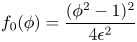 \begin{equation} f_0(\phi)=\frac{(\phi^{2}-1)^{2}}{4\epsilon^{2}} \end{equation}
is the double-well potential, and
 \begin{equation} f_w(\phi)=-\sigma \cos\theta_S\frac{\phi(3-\phi^{2})}{4} \end{equation}
is the surface energy per unit area on the wall (Cahn Reference Cahn1977; Jacqmin Reference Jacqmin2000). Here  $\rho$ is the fluid density,
 $\boldsymbol {u}$ is the fluid velocity,
 $\lambda$ is the mixing energy density,
 $\epsilon$ is the capillary width,
 $\sigma$ is the surface tension and
 $\theta _S$ is the static contact angle (also known as the equilibrium contact angle) defined in fluid 1 (
 $\phi =1$). For a one-dimensional diffuse interface in equilibrium, we have (Yue et al. Reference Yue, Feng, Liu and Shen2004)
 \begin{equation} \sigma =\frac{2\sqrt 2}{3}\frac{\lambda }{\epsilon} \end{equation}
and
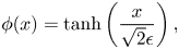 \begin{equation} \phi(x)=\tanh\left(\frac{x}{\sqrt 2 \epsilon}\right), \end{equation}
where we have assumed that the diffuse interface is centred at  $x=0$. The derivation of
 $f_w$ can be found in appendix A.
The free energy (2.1) leads to the following coupled system of Navier–Stokes and Cahn–Hilliard equations:
 \begin{gather} \rho \left( \frac{\partial \boldsymbol{u} }{\partial t} + \boldsymbol{u} \boldsymbol{\cdot} \boldsymbol{\nabla} \boldsymbol{u} \right) + \boldsymbol{J} \boldsymbol{\cdot} \boldsymbol{\nabla} \boldsymbol{u} = -\boldsymbol{\nabla} p + \boldsymbol{\nabla} \boldsymbol{\cdot} \boldsymbol{\tau} + G \boldsymbol{\nabla} \phi + \rho \boldsymbol{g}, \end{gather}
 \begin{gather}\boldsymbol{\nabla} \boldsymbol{\cdot} \boldsymbol{u} = 0, \end{gather}
 \begin{gather}\frac{\partial \phi}{\partial t} + \boldsymbol{u} \boldsymbol{\cdot} \boldsymbol{\nabla} \phi = \boldsymbol{\nabla} \boldsymbol{\cdot} (M \boldsymbol{\nabla} G), \end{gather}
 \begin{gather}G=\lambda(-{\rm \Delta} \phi + f_0'(\phi)) . \end{gather}
Here  $\rho$ is the density,
 $\boldsymbol {u}$ is the volume-averaged velocity,
 $\boldsymbol{J}$ is a diffusive flux caused by the discrepancy between
 $\boldsymbol {u}$ and the mass-averaged velocity (Abels, Garcke & Grün Reference Abels, Garcke and Grün2012),
 $\boldsymbol {\tau }=\mu (\boldsymbol {\nabla } \boldsymbol {u} + (\boldsymbol {\nabla } \boldsymbol {u})^{T})$ is the viscous stress,
 $\mu$ is the viscosity and
 $G$ is the chemical potential. It should be noted that the Cahn–Hilliard equation is split into two second order equations (2.9) and (2.10). This is a common treatment in finite element methods (Yue et al. Reference Yue, Zhou, Feng, Ollivier-Gooch and Hu2006; Khatavkar, Anderson & Meijer Reference Khatavkar, Anderson and Meijer2007b), because the
 $C^{0}$ finite elements cannot handle fourth-order derivatives directly. These equations are complemented by the following boundary conditions:
 \begin{gather} \boldsymbol{u} = \boldsymbol{u}_w \quad \mbox{on }\partial \Omega_w, \end{gather}
 \begin{gather}\boldsymbol{n} \boldsymbol{\cdot} \boldsymbol{\nabla} G = 0\quad \mbox{on }\partial \Omega, \end{gather}
 \begin{gather}\frac{\partial \phi}{\partial t} + \boldsymbol{u} \boldsymbol{\cdot} \boldsymbol{\nabla}\phi = -\Gamma L(\phi,\boldsymbol{\nabla}\phi) \quad \mbox{on } \partial \Omega_w, \end{gather}
 \begin{gather}\boldsymbol{n} \boldsymbol{\cdot} \boldsymbol{\nabla} \phi = 0\quad \mbox{on }\partial\Omega \backslash \partial\Omega_w . \end{gather}
Here  $\boldsymbol {u}_w$ is the wall velocity,
 $\Gamma$ is a positive phenomenological parameter that controls the rate of wall energy relaxation and
 \begin{equation} L(\phi,\boldsymbol{\nabla}\phi)=\lambda \boldsymbol{n} \boldsymbol{\cdot} \boldsymbol{\nabla} \phi + f_w'(\phi) \end{equation}
is the wall potential. Equations (2.11)–(2.13) correspond to the no-slip, zero diffusive flux and wall energy relaxation conditions, respectively. Equation (2.14) corresponds to a homogeneous natural boundary condition, which does not require any special attention in the finite element methods. The interested readers are referred to appendices B and C for the derivation of these equations. On  $\partial \Omega \backslash \partial \Omega _w$, i.e. boundaries other than solid walls, additional velocity or stress conditions are required depending on the particular problem.
In our phase-field formulation,  $\phi$ is related to volume fraction and the mixture properties are computed by
 \begin{equation} \rho(\phi)=\frac{1+\phi}{2}\rho_1+\frac{1-\phi}{2}\rho_2,\quad \mu(\phi)=\frac{1+\phi}{2}\mu_1+\frac{1-\phi}{2}\mu_2, \end{equation}
where subscripts ‘ $_1$’ and ‘
 $_2$’ denote the properties of the pure fluids 1 and 2, respectively. Then, according to (B 13) and (C 4), the diffusive mass flux can be written as
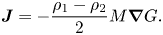 \begin{equation} \boldsymbol{J}=-\frac{\rho_1-\rho_2}{2} M\boldsymbol{\nabla} G. \end{equation}
The wall energy relaxation (2.13), together with the no-slip condition (2.11), is a special case of GNBC. It works together with interface mobility to generate the desired slip length (Yue & Feng Reference Yue and Feng2011). According to Carlson, Do-Quang & Amberg (Reference Carlson, Do-Quang and Amberg2011), the wall energy relaxation accounts for the dissipation due to the reorganization of molecules at the contact line.
For a planar interface,  $\theta _S$ is recovered exactly if
 $L=0$, i.e. when the system is in equilibrium at the contact line. Equation (2.13) allows the contact line to deviate from equilibrium, i.e.
 $L\neq 0$ when the contact line moves. This causes the actual microscopic contact angle measured at the wall (see figure 5b), termed the dynamic contact angle
 $\theta _D$, to deviate from
 $\theta _S$. This deviation has been confirmed by various molecular-dynamics studies (Ren & E Reference Ren and E2007; Fernández-Toledano et al. Reference Fernández-Toledano, Blake, Limat and De Coninck2019). Alternatively, if we assume that the microscopic angle stays at its equilibrium value
 $\theta _S$ then
 $\theta _D$ in the phase-field model can be viewed as the interface angle at a distance of
 $\mathcal {O}(l_D)$ to the contact line, where
 $l_D=\sqrt {M\mu }$ is the diffusion length and
 $\mu$ is an effective viscosity (Yue, Zhou & Feng Reference Yue, Zhou and Feng2010; Yue & Feng Reference Yue and Feng2011). Numerically, this
 $\theta _D$ plays a role similar to the intermediate angle in the macroscale approach of Spelt (Reference Spelt2005) and the numerical angle in the mesh-independent volume-of-fluid method of Afkhami, Zaleski & Bussmann (Reference Afkhami, Zaleski and Bussmann2009). The major difference is that our
 $\theta _D$ is automatically obtained from the phase-field simulations instead of being manually imposed based on external models such as the hydrodynamic model developed by Voinov (Reference Voinov1976) and Cox (Reference Cox1986).
3. Contact angle hysteresis
3.1. Boundary condition for contact angle hysteresis
On the solid wall, the motion of the contact line is directly related to the variation of  $\phi$: the contact line advances if
 ${\textrm {D} \phi }/{\textrm {D}t}>0$ (i.e. the region previously occupied by
 $\phi =-1$ is now occupied by
 $\phi =1$), recedes if
 ${\textrm {D} \phi }/{\textrm {D}t}<0$ and is pinned if
 ${\textrm {D} \phi }/{\textrm {D}t}=0$. Here
 ${\textrm {D}}/{\textrm {D}t}={\partial }/{\partial t} + \boldsymbol {u} \boldsymbol {\cdot } \boldsymbol {\nabla }$ denotes the material derivative and, in particular,
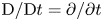 ${\textrm {D}}/{\textrm {D}t}={\partial }/{\partial t}$ on fixed walls. Meanwhile,
 $\theta _D$ is embedded in the
 $\boldsymbol {n}\boldsymbol {\cdot } \boldsymbol {\nabla }\phi$ term of the wall potential
 $L$. We have
 $L<0$ if
 $\theta _D>\theta _S$,
 $L>0$ if
 $\theta _D<\theta _S$ and
 $L=0$ if
 $\theta _D=\theta _S$. Interested readers are referred to appendix A for more details. Thus, we recover the criterion for contact line motion: contact line advances (or recedes) if
 $\theta _D>\theta _S$ (or
 $\theta _D<\theta _S$) and is pinned if
 $\theta _D=\theta _S$.
When CAH exists, the static contact angle has non-unique values, the maximum of which is the advancing contact angle  $\theta _A$ and the minimum of which is the receding contact angle
 $\theta _R$. The contact line advances if
 $\theta _D>\theta _A$, recedes if
 $\theta _D<\theta _R$ and is pinned if
 $\theta _R\le \theta _D \le \theta _A$, as illustrated in figure 1.
Different states of a contact line with CAH. We define the advancing and receding states with respect to the  $\phi =1$ fluid: (a) receding,
 $\theta _D< \theta _R$, (b) pinned,
 $\theta _R\le \theta _D \le \theta _A$ and (c)advancing,
 $\theta _D>\theta _A$.

For convenience, we rewrite the wall energy as
 \begin{equation} f_w(\phi;\theta)=-\sigma\cos \theta \frac{\phi(3-\phi^{2})}{4}, \end{equation}
where the contact angle  $\theta$ is included as a parameter. For the physically relevant range
 $\phi \in [-1,1]$,
 \begin{equation} f_w'(\phi;\theta)=-\frac{3}{4}\sigma \cos \theta (1-\phi^{2}) \end{equation}
is an increasing function in  $\theta$, where
 $'$ denotes the derivative in the first argument. It follows that
 $L(\phi ,\boldsymbol {\nabla }\phi ; \theta )=\lambda \boldsymbol {n} \boldsymbol {\cdot } \boldsymbol {\nabla }\phi + f_w'(\phi ;\theta )$ is also an increasing function in
 $\theta$. For brevity, we denote
 $L(\phi ,\boldsymbol {\nabla }\phi ;\theta _A)$ by
 $L_A$ and
 $L(\phi ,\boldsymbol {\nabla }\phi ;\theta _R)$ by
 $L_R$.
For a contact line with dynamic angle  $\theta _D$, the contact line would be in equilibrium if
 $\theta _D$ were also the static contact angle; it follows that
 $L(\phi ,\boldsymbol {\nabla }\phi ; \theta _D) = 0$, i.e.
 $\lambda \boldsymbol {n}\boldsymbol {\cdot }\boldsymbol {\nabla } \phi = -f_w'(\phi ;\theta _D)$. This is exactly (A 7) in appendix A. Then the relations between
 $\theta _D$,
 $\theta _A$ and
 $\theta _R$ can be mapped to the relations between the wall potentials associated with these angles:
(i) advancing contact line (
 ${\textrm {D} \phi }/{\textrm {D}t}>0) \Leftrightarrow \theta _D>\theta _A>\theta _R \Leftrightarrow 0>L_A>L_R$;
(ii) receding contact line (
${\textrm {D} \phi }/{\textrm {D}t}<0) \Leftrightarrow \theta _A>\theta _R>\theta _D \Leftrightarrow L_A>L_R>0$;(iii) pinned contact line (
${\textrm {D} \phi }/{\textrm {D}t}=0) \Leftrightarrow \theta _A\ge \theta _D\ge \theta _R \Leftrightarrow L_A\ge 0 \ge L_R$.



Apparently, the state (advancing, receding or pinned) of the contact line can be determined by comparing the values of  $L_A$ and
 $L_R$. This motivates the following equation in place of (2.13) on
 $\partial \Omega _w$:
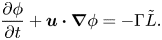 \begin{equation} \frac{\partial \phi}{\partial t} + \boldsymbol{u} \boldsymbol{\cdot} \boldsymbol{\nabla}\phi = - \Gamma \tilde L . \end{equation}
Here
 \begin{equation} \tilde L = \mbox{minmod}(L_A,L_R).\end{equation}
We use the minmod function
 \[ \mbox{minmod}(a,b)=\begin{cases} \mbox{sign}(a)\min(|a|,|b|) & \mbox{if } ab>0,\\ 0 & \mbox{otherwise}, \end{cases} \]
which returns the argument with the smaller magnitude if both arguments have the same sign and zero if otherwise. This equation pins the contact line if  $\theta _D\in [\theta _R,\theta _A]$. If the contact line moves, it automatically picks the correct static contact angle:
 $\theta _A$ if the contact line advances and
 $\theta _R$ if the contact line recedes. It should be noted that, at the leading order, (3.3) is consistent with equation (6) in Prabhala, Panchagnula & Vedantam (Reference Prabhala, Panchagnula and Vedantam2013) for quasi-static computations of drop shapes on hysteric surfaces.
This boundary condition is very easy to implement numerically. In each cell face on the solid wall, we compute the two copies of wall potentials, namely  $L(\phi ,\boldsymbol {\nabla }\phi ;\theta _A)$ and
 $L(\phi ,\boldsymbol {\nabla }\phi ;\theta _R)$. Then we compare the cell average of these two potentials, and decide which one (including 0) we need to take into (3.3). There is no need to extract
 $\theta _D$ or contact line velocity.
3.2. Energy law for contact angle hysteresis
In thermodynamics hysteresis cannot be described by a path-independent state function. Therefore, we cannot find a single-valued wall energy to describe the contact line motion with CAH. However, that does not prevent the system from satisfying a dissipative energy law.
Theorem 3.1 The equation system (2.7)–(2.10), together with the boundary conditions (2.11), (2.12), (2.14) and (3.3), satisfies the energy law
 \begin{equation} \frac{{\rm{d}}}{{\rm{d}}t}\left\{\int_{\Omega} \left(\frac{1}{2}\rho |\boldsymbol{u}|^{2} + f_m\right) {\rm{d}}\boldsymbol{x} + \int_{\partial\Omega_w} f_w(\phi;\theta_A)\,{\rm{d}}s\right\} = {\mathcal{W}} - {\mathcal{D}} -{\mathcal{D}}_{cah}, \end{equation}
where
 \[ {\mathcal{W}} = \oint_{\partial\Omega}{\boldsymbol{n} \boldsymbol{\cdot} \boldsymbol{\mathsf{T}} \boldsymbol{\cdot} \boldsymbol{u}}\,{\rm{d}}s + \int_{\Omega}\rho \boldsymbol{g}\boldsymbol{\cdot} \boldsymbol{u} \,{\rm{d}}\boldsymbol{x} \]
is the power of the reversible work done by the boundary and body force,
 \[ {\mathcal{D}}= \int_\Omega \boldsymbol{\tau}:\boldsymbol{\nabla}\boldsymbol{u}\,{\rm{d}}\boldsymbol{x} +\int_\Omega M |\boldsymbol{\nabla} G|^{2}\,{\rm{d}}\boldsymbol{x} + \int_{\partial\Omega_w}\Gamma \tilde L^{2} \,{\rm{d}}s \ge 0 \]
is the dissipation rate as seen in the standard contact line problem, and
 \[ {\mathcal{D}}_{cah}= \int_{\partial\Omega_w} [\,f_w'(\phi;\theta_R)-f_w'(\phi;\theta_A)] \min\left(\frac{{\rm D} \phi}{{\rm D}t},0\right) \,{\rm{d}}s \ge 0 \]
is the dissipation rate due to CAH. Here  $\boldsymbol{\mathsf{T}} = -p \boldsymbol{\mathsf{I}} +\boldsymbol {\tau } +\boldsymbol {\tau }_\phi$ is the total stress and
 $\boldsymbol {\tau }_\phi$ is given by (B 7). The term in the curly braces is the ‘free energy’ including the kinetic energy, the mixing energy and the wall energy based on the advancing contact angle.
Proof. To save space, we will focus on the proof related to CAH and only provide a sketch for the rest.
From (2.9), (2.16) and (2.17), we recover
 \begin{equation} \frac{\textrm{D}\rho}{\textrm{D}t} = \frac{\rho_1-\rho_2}{2} \frac{\textrm{D} \phi}{\textrm{D}t} =\frac{\rho_1-\rho_2}{2} \boldsymbol{\nabla} \boldsymbol{\cdot} (M\boldsymbol{\nabla} G) = -\boldsymbol{\nabla}\boldsymbol{\cdot} \boldsymbol{J}. \end{equation}
By taking the inner product of (2.7) and  $\boldsymbol {u}$, taking the inner product of (3.6) and
 ${|\boldsymbol {u}|^{2}}/{2}$, and summing them up, we obtain
 \begin{equation} \frac{{\textrm{d}}}{{\textrm{d}}t}\int_{\Omega}\frac{1}{2}\rho |\boldsymbol{u}|^{2}\,{\textrm{d}}\boldsymbol{x} = \oint_{\partial\Omega} \boldsymbol{n} \boldsymbol{\cdot} \boldsymbol{\mathsf{T}} \boldsymbol{\cdot} \boldsymbol{u} \,{\textrm{d}}s+ \int_{\Omega}\rho\boldsymbol{g}\boldsymbol{\cdot} \boldsymbol{u}\,{\textrm{d}}\boldsymbol{x} -\int_{\Omega} \boldsymbol{\mathsf{T}}:\boldsymbol{\nabla} \boldsymbol{u}\,{\rm d}\kern0.5pt \boldsymbol{x}. \end{equation}
Here we have used the incompressibility condition (2.8) and replaced  $G\boldsymbol {\nabla }\phi$ with
 $\boldsymbol {\nabla }\boldsymbol {\cdot } \boldsymbol {\tau }_\phi$ based on the identity (B 19). The derivation of this equation is essentially the same as (C 6). The only difference is that we now include a body force and replace
 $\tilde{\boldsymbol{\mathsf{T}}}$ with
 $\boldsymbol{\mathsf{T}}$.
By taking the inner product of (2.9) and  $G$, taking the inner product of (2.10) with
 $-{\textrm {D} \phi }/{\textrm {D}t}$, and summing them up, we obtain
 \begin{equation} \frac{{\textrm{d}}}{{\textrm{d}}t}\int_{\Omega}f_m\,{\textrm{d}}\boldsymbol{x} = \int_{\partial\Omega_w} \lambda \boldsymbol{n} \boldsymbol{\cdot} \boldsymbol{\nabla}\phi \frac{\textrm{D} \phi}{\textrm{D}t}\,{\textrm{d}}s +\int_\Omega \boldsymbol{\tau}_\phi :\boldsymbol{\nabla}\boldsymbol{u}\,{\textrm{d}}\boldsymbol{x} - \int_\Omega M|\boldsymbol{\nabla}\phi|^{2}\,{\textrm{d}}\boldsymbol{x}, \end{equation}
where we have considered (2.14). The proof of this equation is essentially the reverse of (B 5).
The  $\tilde L$ term in (3.3) takes different values depending on the state of the contact line. If the contact line advances, we have
 ${\textrm {D} \phi }/{\textrm {D}t}={\partial \phi }/{\partial t} + \boldsymbol {u}_w\boldsymbol {\cdot } \boldsymbol {\nabla } \phi >0$ and
 $\tilde L=L_A=\lambda \boldsymbol {n} \boldsymbol {\cdot } \boldsymbol {\nabla }\phi + f_w'(\phi ;\theta _A)$ on
 $\partial \Omega _w$; if the contact line recedes, we have
 ${\textrm {D} \phi }/{\textrm {D}t}<0$ and
 $\tilde L=L_R=\lambda \boldsymbol {n} \boldsymbol {\cdot } \boldsymbol {\nabla }\phi + f_w'(\phi ;\theta _R)$; if the contact line is pinned, we have
 ${\textrm {D} \phi }/{\textrm {D}t}=0$ and
 $\tilde L=0$. This leads to the identity
 \begin{align} \tilde L \frac{\textrm{D} \phi}{\textrm{D}t} & = \lambda \boldsymbol{n} \boldsymbol{\cdot} \boldsymbol{\nabla} \phi \frac{\textrm{D} \phi}{\textrm{D}t} + f_w'(\phi;\theta_A)\max\left(\frac{\textrm{D} \phi}{\textrm{D}t},0\right) + f_w'(\phi;\theta_R)\min\left(\frac{\textrm{D} \phi}{\textrm{D}t},0\right) \nonumber\\ &=\left[ \lambda\boldsymbol{n}\boldsymbol{\cdot} \boldsymbol{\nabla}\phi + f_w'(\phi;\theta_A)\right] \frac{\textrm{D} \phi}{\textrm{D}t}+[\,f_w'(\phi;\theta_R)-f_w'(\phi;\theta_A)]\min\left(\frac{\textrm{D} \phi}{\textrm{D}t},0\right). \end{align}
By taking the inner product of (3.3) and  $-({1}/{\Gamma })({\textrm {D} \phi }/{\textrm {D}t})$ on
 $\partial \Omega _w$, and considering (3.9), we obtain
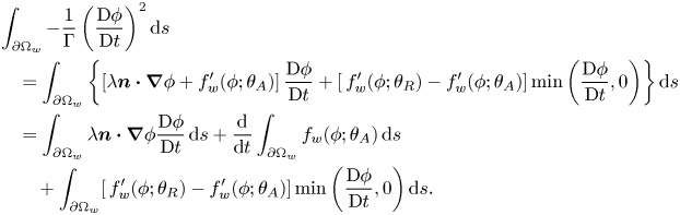 \begin{align} &\int_{\partial\Omega_w} -\frac{1}{\Gamma}\left(\frac{\textrm{D} \phi}{\textrm{D}t}\right)^{2} {\textrm{d}}s \nonumber\\ &\quad = \int_{\partial\Omega_w} \left\{\left[ \lambda\boldsymbol{n}\boldsymbol{\cdot} \boldsymbol{\nabla}\phi + f_w'(\phi;\theta_A)\right] \frac{\textrm{D} \phi}{\textrm{D}t} +[\,f_w'(\phi;\theta_R)-f_w'(\phi;\theta_A)]\min\left(\frac{\textrm{D} \phi}{\textrm{D}t},0\right) \right\}{\textrm{d}}s\nonumber\\ &\quad = \int_{\partial\Omega_w} \lambda \boldsymbol{n} \boldsymbol{\cdot} \boldsymbol{\nabla}\phi \frac{\textrm{D} \phi}{\textrm{D}t} \,{\textrm{d}}s + \frac{{\textrm{d}}}{{\textrm{d}}t}\int_{\partial\Omega_w} f_w(\phi;\theta_A) \,{\textrm{d}}s\nonumber\\ &\qquad + \int_{\partial\Omega_w} [\,f_w'(\phi;\theta_R)-f_w'(\phi;\theta_A)]\min\left(\frac{\textrm{D} \phi}{\textrm{D}t},0\right){\textrm{d}}s. \end{align}
Equation (3.5) can be easily obtained by combining (3.7), (3.8) and (3.10).
The positivity of  ${\mathcal {D}}$ is easily seen. Since
 $\theta _A>\theta _R$, we have
 $f_w'(\phi ;\theta _A)>f_w'(\phi ;\theta _R)$ based on (3.2). Thus, both
 $f_w'(\phi ;\theta _R)-f_w'(\phi ;\theta _A)$ and
 $\min ({\textrm {D} \phi }/{\textrm {D}t},0)$ are non-positive, and
 ${\mathcal {D}}\ge 0$ follows.
Remark 3.1 This theorem neither assumes the fluid domain  $\Omega$ to be fixed, nor does it require
 $\boldsymbol {n}\boldsymbol {\cdot } \boldsymbol {u}=0$ on the boundary. It should be noted that (3.5) can also be cast into
 \begin{equation} \frac{{\textrm{d}}}{{\textrm{d}}t}\left\{\int_{\Omega} \left(\frac{1}{2}\rho |\boldsymbol{u}|^{2} + f_m\right){\textrm{d}}\boldsymbol{x} + \int_{\partial\Omega_w} f_w(\phi;\theta_R)\,{\textrm{d}}s\right\} = {\mathcal{W}} - {\mathcal{D}} -\tilde{{\mathcal{D}}}_{cah}{, }\end{equation}
with
 \[ \tilde{{\mathcal{D}}}_{cah}=\int_{\partial\Omega_w} [\,f_w'(\phi;\theta_A)-f_w'(\phi;\theta_R)] \max\left(\frac{\textrm{D} \phi}{\textrm{D}t},0\right){\textrm{d}}s \ge {0. }\]
It is obvious that  ${\mathcal {D}}_{cah}=0$ if the contact line never recedes and
 $\tilde {{\mathcal {D}}}_{cah}=0$ if the contact line never advances. The dissipation of CAH takes action only when a region on the solid surface is swept by both an advancing contact line and a receding contact line.
It should be noted that the ‘free energy’ in (3.5) can not be understood in the traditional sense. Not all this ‘free energy’ can be used to do work and the portion that can do work is path dependent. For example, if we use  $\theta _A$ to define the wall energy then all the ‘free energy’ can do work if the contact line advances; but if the contact line recedes, only part of the ‘free energy’ can do work and the missing part is
 ${\mathcal {D}}_{cah}$. Similarly, if we use
 $\theta _R$ then only part of the ‘free energy’ can do work when the contact line advances and the missing part is
 $\tilde {{\mathcal {D}}}_{cah}$.
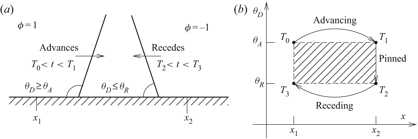
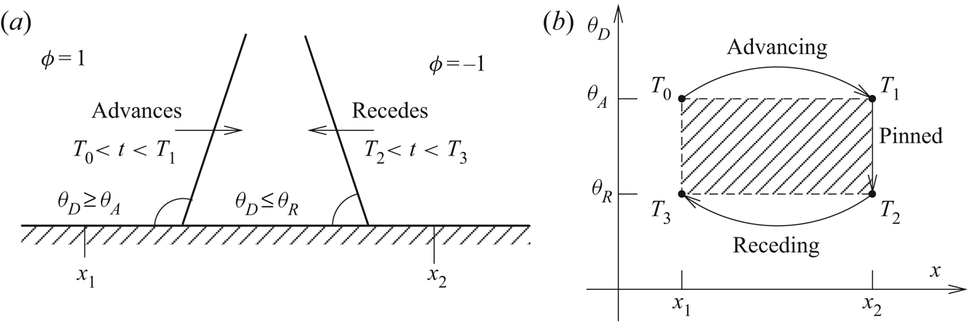
In the following we provide a physical explanation to the dissipation terms that occur on the solid wall. We consider a contact line problem in two dimensions with a stationary solid wall (such that  ${\textrm {D} \phi }/{\textrm {D}t}={\partial \phi }/{\partial t}$) for simplicity. Suppose a contact line advances over a region
 $A=[x_1,x_2]$ with length
 $a=x_2-x_1$ on the solid wall at
 $t\in [T_0,T_3]$, as illustrated in figure 2. At
 $t=T_0$, the contact line starts from
 $x_1$ with
 $\theta _D=\theta _A$. Then the contact line advances with
 $\theta _D\ge \theta _A$ and arrives at
 $x_1$ at
 $t=T_1$. During
 $[T_1,T_2]$ the contact line is pinned at
 $x_2$ and adjusts its microscopic contact angle from
 $\theta _A$ to
 $\theta _R$. Then the contact line recedes with
 $\theta _D\le \theta _R$ and returns to its original position
 $x_1$ at
 $t=T_3$.
Dissipations due to contact line motion. The contact line advances from  $x_1$ to
 $x_2$ and then recedes back to
 $x_1$. (a) Advancing and receding motions of a contact line. (b) Hysteresis loop in the
 $x$–
 $\theta _D$ plane.
In the phase-field context, we have  $\phi =-1$ at
 $t=T_0$,
 $\phi =1$ at
 $t\in [T_1,T_2]$ and
 $\phi =-1$ again at
 $t=T_3$ in
 $A$. Correspondingly,
 ${\partial \phi }/{\partial t}\ge 0$ at
 $t\in [T_0,T_1]$,
 $\partial \phi/\partial t=0$ at
 $t\in [T_1,T_2]$ and
 ${\partial \phi }/{\partial t}\le 0$ at
 $t\in [T_2,T_3]$. Then the energy dissipated due to CAH is
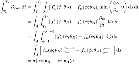 \begin{align} \int_{T_0}^{T_3} {\mathcal{D}}_{cah}\,{\textrm{d}}t &= \int_{T_0}^{T_3} \int_{A} [\,f_w'(\phi;\theta_R)-f_w'(\phi;\theta_A)] \min\left(\frac{\partial\phi}{\partial t},0\right) {\textrm{d}}s \,{\textrm{d}}t \nonumber\\ &= \int_{A} \int_{T_2}^{T_3} [\,f_w'(\phi;\theta_R)-f_w'(\phi;\theta_A)] \frac{\partial\phi}{\partial t}\,{\textrm{d}}t\,{\textrm{d}}s \nonumber\\ &= \int_A \int_{\phi=1}^{\phi=-1} [\,f_w'(\phi;\theta_R)-f_w'(\phi;\theta_A)] \,{\textrm{d}}\phi \,{\textrm{d}}s \nonumber\\ &= \int_A \left[\left. f_w(\phi;\theta_R)\right|_{\phi=1}^{\phi=-1} - \left. f_w(\phi;\theta_A)\right|_{\phi=1}^{\phi=-1}\right] {\textrm{d}}s\nonumber\\ &=\sigma(\cos\theta_R-\cos\theta_A)a, \end{align}
which is non-negative because  $\theta _R\le \theta _A$. This corresponds to the region enclosed by
 $x=x_1$,
 $x=x_2$,
 $\theta _D=\theta _A$ and
 $\theta _D=\theta _R$, which is shaded in figure 2(b). The same amount of dissipation can also be obtained using
 ${\mathcal {D}}^{*}_{cah}$.
Meanwhile, during  $[T_0,T_1]$, the dissipation due to the deviation of
 $\theta _D$ from
 $\theta _A$ is
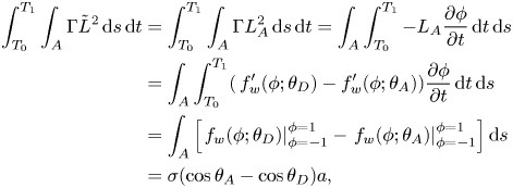 \begin{align} \int_{T_0}^{T_1} \int_A\Gamma \tilde{L}^{2}\,{\textrm{d}}s\,{\textrm{d}}t &=\int_{T_0}^{T_1} \int_A \Gamma L_A^{2}\,{\textrm{d}}s\,{\textrm{d}}t=\int_A \int_{T_0}^{T_1} -L_A \frac{\partial \phi}{\partial t} \,{\textrm{d}}t \,{\textrm{d}}s \nonumber\\ &= \int_A \int_{T_0}^{T_1} (\,f_w'(\phi;\theta_D)-f_w'(\phi;\theta_A)) \frac{\partial \phi}{\partial t}\,{\textrm{d}}t\,{\textrm{d}}s \nonumber \\ &=\int_A \left[\left. f_w(\phi;\theta_D)\right|_{\phi=-1}^{\phi=1} - \left. f_w(\phi;\theta_A)\right|_{\phi=-1}^{\phi=1}\right] {\textrm{d}}s \nonumber\\ &=\sigma(\cos\theta_A-\cos\theta_D)a, \end{align}
where we have used the relation  $\lambda \boldsymbol {n}\boldsymbol {\cdot }\boldsymbol {\nabla }\phi =-f_w'(\phi ;\theta _D)$ (see (A 7)) in the third equality. This corresponds to the region enclosed by the advancing branch of
 $\theta _D$ and
 $\theta _D=\theta _A$ in figure 2(b). It should be noted a tangential force of
 $\sigma \cos \theta _D$ has to be exerted at the contact line in order to move the interface with a contact angle
 $\theta _D$ while the wettability supplies a force of
 $\sigma \cos \theta _A$. The difference between these two forces, which has been referred to as the uncompensated (Qian et al. Reference Qian, Wang and Sheng2003) or unbalanced (Ren & E Reference Ren and E2007) Young's stress in the literature, is responsible for the additional dissipation in (3.13). Similarly, we can get the dissipation due to the deviation of
 $\theta _D$ from
 $\theta _R$ during
 $[T_2,T_3]$, i.e.
 \begin{equation} \int_{T_2}^{T_3} \int_A\Gamma \tilde{L}^{2}\,{\textrm{d}}s\,{\textrm{d}}t = \sigma(\cos\theta_D-\cos\theta_R)a, \end{equation}
which corresponds to the region enclosed by  $\theta _D=\theta _R$ and the receding branch of
 $\theta _D$. A complete hysteresis loop is formed if the contact line stays pinned at
 $x_1$ at
 $t\ge T_3$ and
 $\theta _D$ changes from
 $\theta _R$ to
 $\theta _A$. This pinned state does not cause any dissipation on the solid wall (of course, viscous dissipation in the bulk may be incurred to deform the interface away from the contact line). The argument here can be easily extended to three-dimensional (3-D) flows, where
 $A$ is a two-dimensional (2-D) region on the wall boundary and
 $a$ is the area of
 $A$.
4. Numerical discretization
4.1. Weak form and discrete energy law
The weak form of the governing equations (2.7)–(2.10) and (3.3) can be expressed as
 \begin{align} \left( \rho\frac{D \boldsymbol{u}}{D t} + \boldsymbol{J} \boldsymbol{\cdot} \boldsymbol{\nabla} \boldsymbol{u}, \hat{\boldsymbol{u}} \right) &= \left(\boldsymbol{n} \boldsymbol{\cdot} (-p \boldsymbol{\mathsf{I}} + \boldsymbol{\tau}),\hat{\boldsymbol{u}}\right)_{\partial\Omega} - \left(-p \boldsymbol{\mathsf{I}} + \boldsymbol{\tau}, \boldsymbol{\nabla} \hat{\boldsymbol{u}}\right) \nonumber\\ &\quad +(G\boldsymbol{\nabla}\phi +\rho \boldsymbol{g}, \hat{\boldsymbol{u}}), \end{align}
 \begin{gather} -\left(\boldsymbol{\nabla}\boldsymbol{\cdot} \boldsymbol{u}, \hat p\right) =0, \end{gather}
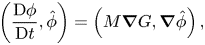 \begin{gather}\left(\frac{\textrm{D} \phi}{\textrm{D}t},\hat \phi \right) = \left( M \boldsymbol{\nabla} G, \boldsymbol{\nabla} \hat\phi\right), \end{gather}
 \begin{gather}\left(G,\hat G\right) -\frac{1}{\Gamma}\left(\frac{\textrm{D} \phi}{\textrm{D}t}, \hat G\right)_{\partial\Omega_w} = (\lambda \boldsymbol{\nabla}\phi, \boldsymbol{\nabla} \hat G) +(\lambda f_0'(\phi), \hat G) + \left(A,\hat G\right)_{\partial\Omega_w}, \end{gather}
where  $(\cdot ,\cdot )$ denotes the
 $L_2$ inner product in the domain
 $\Omega$,
 $(\cdot ,\cdot )_{\partial \Omega }$ and
 $(\cdot ,\cdot )_{\partial \Omega _w}$ denote the inner product on
 $\partial \Omega$ and
 $\partial \Omega _w$. We seek solutions
 $\boldsymbol {u}\in H^{1}(\Omega )^{d}$,
 $p\in L^{2}(\Omega )$,
 $\phi \in H^{1}(\Omega )$ and
 $G \in H^{1}(\Omega )$ satisfying the equations above, where
 $d$ is the dimension of the problem. The variables with
 $\hat {}$ are the corresponding test functions. The special form of (4.4) is motivated by the proof of Theorem 3.1. The
 $\lambda \boldsymbol {n}\boldsymbol {\cdot }\boldsymbol {\nabla }\phi$ term in
 $\tilde L$ is cancelled out on
 $\partial \Omega _w$ unless the contact line is pinned. The term
 $A$ comes from CAH and can be expressed as
 \begin{equation} A=\begin{cases} f_w'(\phi;\theta_A)= -\frac{3}{4}\sigma\cos\theta_A (1-\phi^{2}) & \mbox{ if } 0\ge L_A\ge L_R \mbox{ (contact line advances)},\\ f_w'(\phi;\theta_R)=-\frac{3}{4}\sigma\cos\theta_R (1-\phi^{2}) & \mbox{ if } L_A\ge L_R>0 \mbox{ (contact line recedes)},\\ -\lambda \boldsymbol{n} \boldsymbol{\cdot} \boldsymbol{\nabla}\phi & \mbox{ otherwise}. \end{cases} \end{equation}
If  $\boldsymbol {\nabla }\boldsymbol {\cdot }\boldsymbol {u}=0$ is satisfied in the strong sense then the energy law (3.5) is recovered if we take
 $\hat{\boldsymbol {u}} =\boldsymbol {u}$,
 $\hat \phi =G$ and
 $\hat G={\textrm {D} \phi }/{\textrm {D}t}$. To obtain a similar energy law under the weak incompressibility condition (4.2), special care must be taken on the momentum equation, e.g. the skew-symmetric form for flows with constant density and the method of Guermond& Quartapelle (Reference Guermond and Quartapelle2000) for flows with variable density.
There have been energy stable numerical schemes for moving contact line problems with variable densities (e.g. Gao & Wang Reference Gao and Wang2014; Yu & Yang Reference Yu and Yang2017; Metzger Reference Metzger2019). But they are all first order in time and the time step has to be very small for reasonable temporal accuracy. In this work we adopt a second-order time discretization based on the Crank–Nicolson method and a skew-symmetric form for the convection term in the momentum equation. In the semi-discrete form, we seek  $\boldsymbol {u}^{{n+1}}$,
 $p^{{n+{1}/{2}}}$,
 $\phi ^{{n+1}}$ and
 $G^{{n+{1}/{2}}}$ satisfying
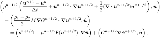 \begin{align} &\left(\rho^{{n+{1}/{2}}} \left(\frac{\boldsymbol{u}^{{n+1}}-\boldsymbol{u}^{n}}{{\rm \Delta} t} +\bar{\boldsymbol{u}}^{{n+{1}/{2}}} \boldsymbol{\cdot} \boldsymbol{\nabla} \boldsymbol{u}^{{n+{1}/{2}}} +\frac{1}{2} (\boldsymbol{\nabla}\boldsymbol{\cdot} \bar{\boldsymbol{u}}^{{n+{1}/{2}}}) \boldsymbol{u}^{{n+{1}/{2}}}\right), \hat{\boldsymbol{u}}\right)\nonumber\\ &\quad -\left(\frac{\rho_1-\rho_2}{2} M \boldsymbol{\nabla} G^{{n+{1}/{2}}} \boldsymbol{\cdot} \boldsymbol{\nabla}\boldsymbol{u}^{{n+{1}/{2}}},\hat{\boldsymbol{u}} \right)\nonumber\\ &\qquad =\left(p^{{n+{1}/{2}}} \boldsymbol{\mathsf{I}}-\mu^{{n+{1}/{2}}} {\boldsymbol{\mathsf{E}}}(\boldsymbol{u}^{{n+{1}/{2}}}), \boldsymbol{\nabla} \hat{\boldsymbol{u}}\right) + \left(G^{{n+{1}/{2}}} \boldsymbol{\nabla}\phi^{{n+{1}/{2}}}, \hat{\boldsymbol{u}}\right), \end{align}
 \begin{equation} -\left(\boldsymbol{\nabla} \boldsymbol{\cdot} \boldsymbol{u}^{n}, \hat p\right)=0 , \end{equation}
 \begin{equation}\left(\frac{\phi^{n+1}-\phi^{n}}{{\rm \Delta} t} + \boldsymbol{u}^{{n+{1}/{2}}}\boldsymbol{\cdot}\boldsymbol{\nabla}\phi^{{n+{1}/{2}}}, \hat \phi\right)=(-M\boldsymbol{\nabla} G^{{n+{1}/{2}}},\boldsymbol{\nabla} \hat\phi), \end{equation}
 \begin{align} &(G^{{n+{1}/{2}}},\hat G)-\left(\frac{1}{\Gamma}\left(\frac{\phi^{{n+1}}-\phi^{n}}{{\rm \Delta} t}+\boldsymbol{u}_w\boldsymbol{\cdot} \boldsymbol{\nabla} \phi^{{n+{1}/{2}}} \right),\hat G\right)_{\partial\Omega_w}\nonumber\\ &\quad =\left(\lambda \boldsymbol{\nabla} \phi^{{n+{1}/{2}}},\boldsymbol{\nabla} \hat G\right) + \left(\lambda Df_0(\phi^{n},\phi^{{n+1}}), \hat G\right) + \sum_{e\in \mathcal{T}(\partial\Omega_w)}\left(A^{{n+{1}/{2}}},\hat G\right)_e, \end{align}
for all admissible test functions  $\hat{\boldsymbol {u}} $,
 $\hat p$,
 $\hat \phi$ and
 $\hat G$. Here,
 ${\rm \Delta} t =t^{{n+1}}-t^{n}$ is the time step,
 $\boldsymbol {u}^{{n+{1}/{2}}}={(\boldsymbol {u}^{{n+1}}+\boldsymbol {u}^{n})}/{2}$ and
 $\phi ^{{n+{1}/{2}}}={(\phi ^{{n+1}}+\phi ^{n})}/{2}$ are second-order approximations at half-time level
 $t^{{n+{1}/{2}}}$,
 $\bar{\boldsymbol {u}}^{{n+{1}/{2}}}={(3 \boldsymbol {u}^{n}-\boldsymbol {u}^{n-1})}/{2}$ (
 $\bar{\boldsymbol {u}}^{{n+{1}/{2}}}=\boldsymbol {u}^{n}$ for
 $n=0$) is an explicit approximation at
 $t^{{n+{1}/{2}}}$ by extrapolation,
 \[ \rho^{{n+{1}/{2}}}=\frac{1+\phi^{{n+{1}/{2}}}}{2}\rho_1+\frac{1-\phi^{{n+{1}/{2}}}}{2}\rho_2,\quad \mu^{{n+{1}/{2}}}=\frac{1+\phi^{{n+{1}/{2}}}}{2}\mu_1+\frac{1-\phi^{{n+{1}/{2}}}}{2}\mu_2, \]
 $\mathcal {T}(\partial \Omega _w)$ denotes the triangulation of the wall boundary
 $\partial \Omega _w$ and
 $e$ denotes an element face (or edge in two dimensions) on
 $\partial \Omega _w$. We have also introduced the strain rate tensor
 $\boldsymbol{\mathsf{E}}(\boldsymbol {u})=\boldsymbol {\nabla }\boldsymbol {u} + (\boldsymbol {\nabla }\boldsymbol {u})^{T}$ for convenience. The term
 $Df_0$, first introduced by Du & Nicolaides (Reference Du and Nicolaides1991) and sometimes referred to as the discrete variational derivative (Gomez & van der Zee Reference Gomez and van der Zee2017), is a second-order approximation to
 $f_0'(\phi ^{{n+{1}/{2}}})$ for the purpose of energy stability:
 \begin{equation} Df_0(\phi^{n},\phi^{{n+1}}) =\begin{cases} \dfrac{f_0(\phi^{{n+1}})-f_0(\phi^{n})}{\phi^{{n+1}}-\phi^{n}} & \mbox{if } \phi^{{n+1}}\neq \phi^{n}, \\ f_0'(\phi^{n}) & \mbox{if } \phi^{{n+1}}=\phi^{n}. \end{cases} \end{equation}
The term  $A^{{n+{1}/{2}}}$ takes care of CAH. For the convenience of numerical implementation, we determine the status of the contact line by comparing the integral of wall potential. On each element face
 $e$ on the wall boundary, we have
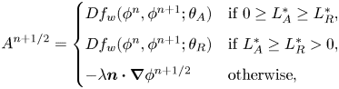 \begin{equation} A^{{n+{1}/{2}}}=\begin{cases} Df_w(\phi^{n},\phi^{{n+1}};\theta_A) & \mbox{if } 0\ge L^{*}_A\ge L^{*}_R,\\ Df_w(\phi^{n},\phi^{{n+1}};\theta_R) & \mbox{if } L^{*}_A\ge L^{*}_R>0,\\ -\lambda \boldsymbol{n} \boldsymbol{\cdot} \boldsymbol{\nabla}\phi^{{n+{1}/{2}}} & \mbox{otherwise}, \end{cases} \end{equation}
where  $Df_w$ is the discrete variational derivative of
 $f_w$.
 $L^{*}_A$ and
 $L^{*}_R$ are the integrals of wall potentials on the element face and they are defined explicitly for numerical convenience:
 $L^{*}_{A,R}=\int _e[\lambda \boldsymbol {n} \boldsymbol {\cdot } \boldsymbol {\nabla }\phi ^{n} + f_w'(\phi ^{n};\theta _{A,R}) ]\,{\textrm {d}}s$.
In most problems we impose either a zero traction condition  $\boldsymbol {n}\boldsymbol {\cdot } {\boldsymbol{\mathsf{T}}} = \boldsymbol {0}$ or a Dirichlet condition for
 $\boldsymbol {u}$ on the domain boundary, which causes the surface integral term in (4.1) to vanish. Thus, for brevity, the surface integral term is dropped in (4.6).
This scheme does not have unconditional energy stability, but it satisfies the following discrete energy law for matched density.
Theorem 4.1 If  $\rho _1=\rho _2=\rho$ and
 $\boldsymbol {u}_w=0$, then the semi-discrete system (4.6)–(4.9) with the non-penetrating essential boundary condition
 $\boldsymbol {n} \boldsymbol {\cdot } \boldsymbol {u}|_{{{\partial \Omega }}} =0$ satisfies the discrete energy law
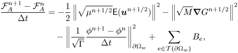 \begin{align} \frac{\mathcal{F}_A^{{n+1}}-\mathcal{F}_A^{n}}{{\rm \Delta} t} &= - \frac{1}{2}\left\|\sqrt{\mu^{{n+{1}/{2}}}} \boldsymbol{\mathsf{E}}(\boldsymbol{u}^{{n+{1}/{2}}})\right\|^{2}-\left\|\sqrt M\boldsymbol{\nabla} G^{{n+{1}/{2}}}\right\|^{2}\nonumber\\ &\quad - \left\| \frac{1}{\sqrt \Gamma} \frac{\phi^{{n+1}}-\phi^{n}}{{\rm \Delta} t}\right\|^{2}_{\partial\Omega_w}+\sum_{e\in \mathcal{T} (\partial\Omega_w)} B_e {, } \end{align}
where
 \begin{equation} \mathcal{F}_A^{n}= \int_{\Omega} \left[\frac{1}{2}\rho|\boldsymbol{u}^{n}|^{2} + \lambda\left(\frac{1}{2}|\boldsymbol{\nabla}\phi^{n}|^{2} + f_0(\phi^{n})\right)\right]{\rm{d}}\boldsymbol{x} + \int_{\partial\Omega_w} f_w(\phi^{n};\theta_A) \,{\rm{d}}s \end{equation}
and
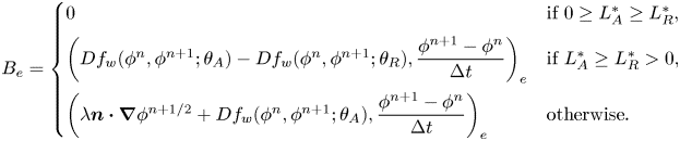 \begin{equation} B_e=\begin{cases} 0 & \mbox{if } 0\ge L^{*}_A\ge L^{*}_R, \\ \left(Df_w(\phi^{n},\phi^{{n+1}};\theta_A) -Df_w(\phi^{n},\phi^{{n+1}};\theta_R),\dfrac{\phi^{{n+1}}-\phi^{n}}{{\rm \Delta} t} \right)_e & \mbox{if } L^{*}_A\ge L^{*}_R>0,\\ \left(\lambda\boldsymbol{n}\boldsymbol{\cdot} \boldsymbol{\nabla}\phi^{{n+{1}/{2}}} + Df_w(\phi^{n},\phi^{{n+1}};\theta_A), \dfrac{\phi^{{n+1}}-\phi^{n}}{{\rm \Delta} t}\right)_e & \mbox{otherwise}. \end{cases} \end{equation}
Proof. Taking  $\hat{\boldsymbol {u}} =\boldsymbol {u}^{{n+{1}/{2}}}$, the left-hand side (LHS) of (4.6) becomes
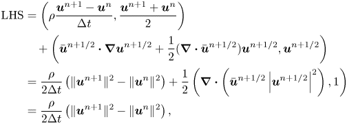 \begin{align} \textrm{LHS} &= \left(\rho\frac{\boldsymbol{u}^{{n+1}}-\boldsymbol{u}^{n}}{{\rm \Delta} t},\frac{\boldsymbol{u}^{{n+1}}+\boldsymbol{u}^{n}}{2}\right) \nonumber\\ &\quad +\left(\bar{\boldsymbol{u}}^{{n+{1}/{2}}} \boldsymbol{\cdot} \boldsymbol{\nabla} \boldsymbol{u}^{{n+{1}/{2}}} +\frac{1}{2} (\boldsymbol{\nabla}\boldsymbol{\cdot} \bar{\boldsymbol{u}}^{{n+{1}/{2}}}) \boldsymbol{u}^{{n+{1}/{2}}},\boldsymbol{u}^{{n+{1}/{2}}}\right) \nonumber\\ &=\frac{\rho}{2{\rm \Delta} t} \left(\|\boldsymbol{u}^{{n+1}}\|^{2}-\|\boldsymbol{u}^{n}\|^{2}\right) + \frac{1}{2}\left(\boldsymbol{\nabla}\boldsymbol{\cdot}\left(\bar{\boldsymbol{u}}^{{n+{1}/{2}}} \left|\boldsymbol{u}^{{n+{1}/{2}}}\right|^{2}\right),1\right) \nonumber\\ &= \frac{\rho}{2{\rm \Delta} t} \left(\|\boldsymbol{u}^{{n+1}}\|^{2}-\|\boldsymbol{u}^{n}\|^{2}\right), \end{align}
where we have used the boundary condition  $\bar{\boldsymbol {u}}^{{n+{1}/{2}}}\boldsymbol {\cdot }\boldsymbol {n}|_{{\partial \Omega }}={(3\boldsymbol {u}^{{n+1}}-\boldsymbol {u}^{n})}/{2}\boldsymbol {\cdot }\boldsymbol {n}|_{{\partial \Omega }} = \boldsymbol {0}$ in the last equality. It should be noted that this equation does not require
 $\boldsymbol {\nabla }\boldsymbol {\cdot }\boldsymbol {u}^{n}=0$ to be exactly satisfied. The right-hand side (RHS) of (4.6) becomes
 \begin{align} \textrm{RHS} & = \left(p^{{n+{1}/{2}}}, \boldsymbol{\nabla}\boldsymbol{\cdot} \boldsymbol{u}^{{n+{1}/{2}}}\right)-\left(\mu^{{n+{1}/{2}}} \boldsymbol{\mathsf{E}}(\boldsymbol{u}^{{n+{1}/{2}}}), \boldsymbol{\nabla}\boldsymbol{u}^{{n+{1}/{2}}}\right) +\left(G^{{n+{1}/{2}}}\boldsymbol{\nabla}\phi^{{n+{1}/{2}}},\boldsymbol{u}^{{n+{1}/{2}}}\right)\nonumber\\ &= \left(p^{{n+{1}/{2}}}, \boldsymbol{\nabla}\boldsymbol{\cdot} \boldsymbol{u}^{{n+{1}/{2}}}\right) - \|\sqrt{\mu^{{n+{1}/{2}}}} \boldsymbol{\mathsf{E}}(\boldsymbol{u}^{{n+{1}/{2}}})\|^{2} + \left(G^{{n+{1}/{2}}}\boldsymbol{\nabla}\phi^{{n+{1}/{2}}},\boldsymbol{u}^{{n+{1}/{2}}}\right). \end{align}
Since (4.7) is satisfied at each time level, it follows that  $-(\boldsymbol {\nabla }\boldsymbol {\cdot } ({(\boldsymbol {u}^{{n+1}}+\boldsymbol {u}^{n})}/{2}),\hat p)=0$. By taking
 $\hat p=p^{{n+{1}/{2}}}$, we obtain
 \begin{equation} -\left(\boldsymbol{\nabla}\boldsymbol{\cdot}\boldsymbol{u}^{{n+{1}/{2}}}, p^{{n+{1}/{2}}}\right)=0. \end{equation}
By taking  $\hat \phi =G^{{n+{1}/{2}}}$, (4.8) leads to
 \begin{equation} \left(\frac{\phi^{{n+1}}-\phi^{n}}{{\rm \Delta} t}, G^{{n+{1}/{2}}}\right) + \left(\boldsymbol{u}^{{n+{1}/{2}}}\boldsymbol{\cdot}\boldsymbol{\nabla}\phi^{{n+{1}/{2}}}, G^{{n+{1}/{2}}}\right) = -\left(M\boldsymbol{\nabla} G^{{n+{1}/{2}}},\boldsymbol{\nabla} G^{{n+{1}/{2}}}\right). \end{equation}
We then take  $\hat G={(\phi ^{{n+1}}-\phi ^{n})}/{{\rm \Delta} t}$ in (4.9) and obtain
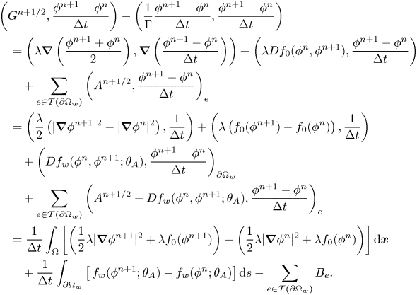 \begin{align} &\left(G^{{n+{1}/{2}}},\frac{\phi^{{n+1}}-\phi^{n}}{{\rm \Delta} t}\right) -\left(\frac{1}{\Gamma}\frac{\phi^{{n+1}}-\phi^{n}}{{\rm \Delta} t},\frac{\phi^{{n+1}}-\phi^{n}}{{\rm \Delta} t}\right) \nonumber\\ &\quad =\left(\lambda\boldsymbol{\nabla}\left(\frac{\phi^{{n+1}}+\phi^{n}}{2}\right), \boldsymbol{\nabla} \left(\frac{\phi^{{n+1}}-\phi^{n}}{{\rm \Delta} t}\right)\right) + \left(\lambda Df_0(\phi^{n},\phi^{{n+1}}), \frac{\phi^{{n+1}}-\phi^{n}}{{\rm \Delta} t}\right) \nonumber\\ &\qquad + \sum_{e\in \mathcal{T} (\partial\Omega_w)}\left(A^{{n+{1}/{2}}}, \frac{\phi^{{n+1}}-\phi^{n}}{{\rm \Delta} t}\right)_e \nonumber\\ &\quad =\left(\frac{\lambda}{2}\left(|\boldsymbol{\nabla}\phi^{{n+1}}|^{2}-|\boldsymbol{\nabla}\phi^{n}|^{2}\right),\frac{1}{{\rm \Delta} t}\right)+ \left(\lambda\left(f_0(\phi^{{n+1}})-f_0(\phi^{n})\right),\frac{1}{{\rm \Delta} t}\right)\nonumber\\ &\qquad + \left(Df_w(\phi^{n},\phi^{{n+1}};\theta_A),\frac{\phi^{{n+1}}-\phi^{n}}{{\rm \Delta} t}\right)_{\partial\Omega_w} \nonumber\\ &\qquad +\sum_{e\in \mathcal{T} (\partial\Omega_w)}\left(A^{{n+{1}/{2}}}-Df_w(\phi^{n},\phi^{{n+1}};\theta_A), \frac{\phi^{{n+1}}-\phi^{n}}{{\rm \Delta} t}\right)_e \nonumber \\ &\quad = \frac{1}{{\rm \Delta} t}\int_\Omega \left[\left(\frac{1}{2}\lambda|\boldsymbol{\nabla}\phi^{{n+1}}|^{2} +\lambda f_0(\phi^{{n+1}})\right)-\left(\frac{1}{2}\lambda|\boldsymbol{\nabla}\phi^{n}|^{2} +\lambda f_0(\phi^{n})\right)\right]{\textrm{d}}\boldsymbol{x} \nonumber\\ &\qquad +\frac{1}{{\rm \Delta} t} \int_{\partial\Omega_w} \left[\,f_w(\phi^{{n+1}};\theta_A)-f_w(\phi^{n};\theta_A)\right]{\textrm{d}}s - \sum_{e\in \mathcal{T} (\partial\Omega_w)} B_e. \end{align}
Finally, by summing up equations (4.15)–(4.18) and subtracting (4.19), we arrive at (4.12).
Remark 4.1 Since the proof is based on weak form and integration by parts, it can be easily extended to Galerkin methods with finite-dimensional function spaces (Shen et al. Reference Shen, Yang and Yu2015). This energy law thus also applies to the fully discrete Galerkin finite element methods. The only additional requirement is that  $\phi$ and
 $G$ must share the same function space such that we can take
 $\hat \phi =G^{n+1/2}$ and
 $\hat G={(\phi ^{n+1}-\phi ^{n})}/{{\rm \Delta} t}$.
Remark 4.2 The energy law (4.12) is dissipative except for the  $B_e$ term due to hystersis. We cannot prove this term to be non-positive from the weak form. However, we can show
 $B_e\le 0$ if the strong form (3.3) is satisfied.
(i) If
$0>L^{*}_A>L^{*}_R$, the contact line advances and we have the trivial relation $B_e=0$.(ii) If
$L^{*}_A>L^{*}_R>0$, the contact line recedes according to the strong form (3.3) and, thus, $\phi ^{{n+1}}-\phi ^{n}\le 0$. Similar to the inequality $f_w'(\phi ,\theta _A)\ge f_w'(\phi ;\theta _R)$, it can be easily shown that $Df_w(\phi ^{n},\phi ^{{n+1}};\theta _A)\ge Df_w(\phi ^{n},\phi ^{{n+1}}; \theta _R)$ for $\phi ^{n},\phi ^{{n+1}}\in [-1,1]$. Thus, we have $B_e\le 0$ when the contact line recedes. This corresponds to the dissipation term ${\mathcal {D}}_{cah}$ in Theorem 3.1.(iii) Otherwise, the contact line is pinned according to (3.3). In this case
$\phi ^{{n+1}}=\phi ^{n}$ and, thus, $B_e=0$.
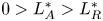

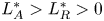






It should be noted, however, that the weak form cannot exactly guarantee  $\phi ^{{n+1}}>\phi ^{n}$ when
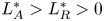 $L^{*}_A>L^{*}_R>0$ or
 $\phi ^{{n+1}}=\phi ^{n}$ when
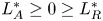 $L^{*}_A\ge 0 \ge L^{*}_R$. Thus, there might be regions with
 $Be > 0$ on wall boundaries in finite element computations. But, in practice, we do expect the weak solution to be a reasonable approximation to the strong solution and thus
 $B_e\le 0$ to be ‘approximately’ satisfied.
Remark 4.3 In the absence of CAH, we have  $\theta _A=\theta _R$ and, thus,
 $B_e=0$. In this case, (4.12) recovers unconditional energy stability. It should be noted, however, that our numerical scheme is nonlinear and requires iterations. Thus, the time step still cannot be too large in practical computations.
Although we can not establish the energy stability for variable density problems, it does not raise severe stability concerns in practical computations as demonstrated later in § 5.3.
4.2. Numerical methods
The equation system (4.6)–(4.9) are solved by the finite element method using the deal.ii library (Bangerth, Hartmann & Kanschat Reference Bangerth, Hartmann and Kanschat2007; Alzetta et al. Reference Alzetta, Arndt, Bangerth, Boddu, Brands, Davydov, Gassmoeller, Heister, Heltai and Kormann2018). Hierarchical adaptive meshes, quadrilateral in two dimensions and hexagonal in three dimensions, are used to discretize the computational domain. We use  $Q2$ elements for
 $\boldsymbol {u}$,
 $Q1$ elements for
 $p$ and
 $Q3$ elements for
 $\phi$ and
 $G$. For easy implementation, we solve the flow equations (4.6) and (4.7) separately from the Cahn–Hilliard equations (4.8) and (4.9), and then couple them together using a Picard iteration.
The nonlinear system of (4.8) and (4.9) are solved by Newton's method. On each element face  $e$ on
 $\partial \Omega _w$, we compute two copies of chemical potential
 $L_A$ and
 $L_R$, and their integrals
 $L^{*}_A$ and
 $L^{*}_R$ on
 $e$. The value of
 $A^{{n+{1}/{2}}}$ is then determined from (4.11). The linear system in each Newton step is solved by the generalized minimal residual method (GMRES) with the incomplete LU factorization (ILU) preconditioner.
The momentum equation (4.6) and the continuity equation (4.7) are solved by the mixed finite element method. Thanks to the explicit  $\bar{\boldsymbol {u}}^{{n+{1}/{2}}}$, we have the linear saddle point system
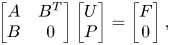 \begin{equation} \begin{bmatrix}A & B^{T} \\ B & 0\end{bmatrix} \begin{bmatrix}U \\ P\end{bmatrix} =\begin{bmatrix}F\\0\end{bmatrix}, \end{equation}
where  $U$ and
 $P$ are solutions vectors for
 $\boldsymbol {u}^{{n+1}}$ and
 $p^{{n+{1}/{2}}}$, respectively. The asymmetric block
 $A$ comes from the momentum equation except for the pressure term and the block
 $B$ comes from the continuity equation. For 2-D problems, where the number of degrees of freedom is typically below one million, we solve this system by the direct sparse linear solver UMFPACK (Davis Reference Davis2004). For 3-D problems, we adopt the grad-div stabilization and solve the saddle point system by GMRES with a block-triangular Schur complement preconditioner developed by Heister & Rapin (Reference Heister and Rapin2013). Detailed implementation of this preconditioner can be found in tutorial step-57 of deal.ii.
The solution procedure can be summarized as follows.
(i) Create an initial mesh which is refined at the interface and set the initial data
$\boldsymbol {u}^{0}$ and $\phi ^{0}$.(ii) For each time step
$n\ge 0$, choose a proper ${\rm \Delta} t$ and perform the following steps until the stopping time is reached.
(a) Based on
$\phi ^{n}$, locally refine or coarsen the mesh such that the mesh is the finest at the interface with $h_{min} \in [0.5\epsilon ,\epsilon ]$ and gets coarsened away from the interface. Transfer data from the old mesh to the new mesh if the mesh is modified.(b) Let
$k$ denote the iteration step. Set $k=0$ and $\boldsymbol {u}^{{{n+{1}/{2}}},0}=\bar{\boldsymbol {u}}^{{n+{1}/{2}}}$, and iterate over the following steps until convergence.
(1) Solve the Cahn–Hilliard equations (4.8) and (4.9) for
$\phi ^{{{n+1}},k+1}$ and $G^{{{n+{1}/{2}}},k+1}$ based on $\phi ^{n}$ and $\boldsymbol {u}^{{{n+{1}/{2}}},k}$.(2) Solve the flow equations (4.6) and (4.7) for
$\boldsymbol {u}^{{{n+1}},k+1}$ and $p^{{{n+{1}/{2}}},k+1}$ based on $\boldsymbol {u}^{n}$, $\bar{\boldsymbol {u}}^{{n+{1}/{2}}}$, $\phi ^{{{n+{1}/{2}}},k+1}$ and $G^{{{n+{1}/{2}}},k+1}$.(3) Set
$k=k+1$.
(c) Update solution at
$t^{n+1}$: $\boldsymbol {u}^{{n+1}}=\boldsymbol {u}^{{{n+1}},k}$, $p^{{n+{1}/{2}}}=p^{{{n+{1}/{2}}},k}$, $\phi ^{{n+1}}=\phi ^{{{n+1}},k}$ and $G^{{n+{1}/{2}}}=G^{nh,k}$.












In practice we only need a few iterations in (iib). For the computationally expensive 3-D problems, we only compute two iterations, i.e. up to  $k=2$.
5. Results and discussions
5.1. Drop deformation in plane Poiseuille flow
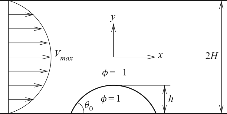
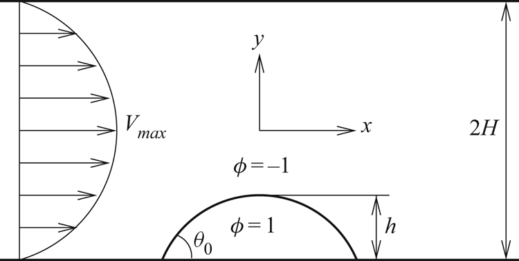
We first validate our method by computing the drop deformation with pinned contact lines in plane Poiseuille flow (Schleizer & Bonnecaze Reference Schleizer and Bonnecaze1999). This 2-D test case has been widely used for validation purpose (e.g. Spelt Reference Spelt2005; Dupont & Legendre Reference Dupont and Legendre2010; Huang et al. Reference Huang, Huang and Wang2014; Liu et al. Reference Liu, Ju, Wang, Xi and Zhang2015). The computational domain is a  $8H\times 2H$ rectangle with a drop adhered to the lower wall, as shown in figure 3(a). At the inlet, we impose a fully developed flow velocity
 $u=[1-({y}/{H})^{2}]V_{max}$, where
 $V_{max}$ is the maximum velocity along the centreline of the channel. At the outlet, we impose the zero traction condition. The lower and upper boundaries are stationary walls, where the velocity is set to zero. A drop is placed on the lower wall. Initially, the drop is a circular segment with contact angle
 $\theta _0=60^{\circ }$. The drop has radius
 $R_0=0.9023H$ and height
 $h=0.4511H$, such that its area is
 $0.5H^{2}$. Inertia is neglected and the viscosity ratio is unity, i.e.
 $\mu _1=\mu _2=\mu$. Following Schleizer & Bonnecaze (Reference Schleizer and Bonnecaze1999), we define the characteristic shear rate
 $E={\partial u}/{\partial y} |_{y=-H}={2V_{max}}/{H}$ and the capillary number
 $Ca={\mu Eh}/{\sigma } =({\mu V_{max}}/{\sigma })({2h}/{H})$. To pin the contact line, we set
 $\theta _A=170^{\circ }$ and
 $\theta _R=10^{\circ }$.
Schematic of a drop under shear in plane Poiseuille flow.
For the Cahn–Hilliard equation, we introduce the following dimensionless parameters (Yue et al. Reference Yue, Zhou and Feng2010; Yue & Feng Reference Yue and Feng2011): the Cahn number
 \begin{equation} Cn=\frac{\epsilon}{H} \end{equation}
that characterizes the thickness of the interface,
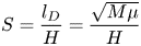 \begin{equation} S=\frac{l_D}{H}=\frac{\sqrt{M\mu}}{H} \end{equation}
that characterizes the slip due to Cahn–Hilliard diffusion, and
 \begin{equation} \Pi=\frac{1}{\mu\Gamma H} \end{equation}
that characterizes the wall energy relaxation rate. Here  $l_D=\sqrt {M\mu }$ is the diffusion length in the phase-field method, which is the counterpart of slip length in the slip models. For this test case, we choose
 $Cn=0.01$,
 $S=0.01$ and
 $\Pi =0.1$. The computational mesh is adaptively refined at the interface and the mesh sizes are
 $h_{min}={H}/{128}$ at the interface and
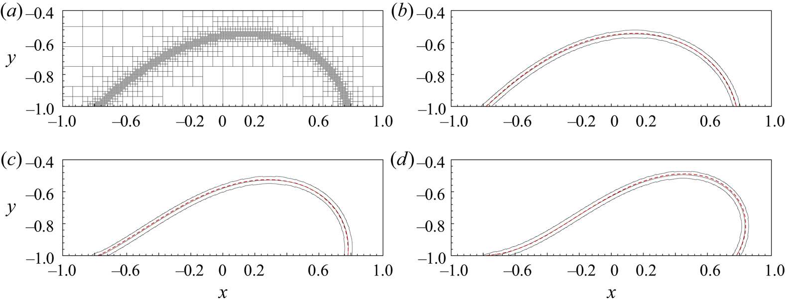
 $h_{max}={H}/{8}$ in the bulk phases, as shown in figure 4(a). There are typically five layers of mesh cells in the diffuse interface (between
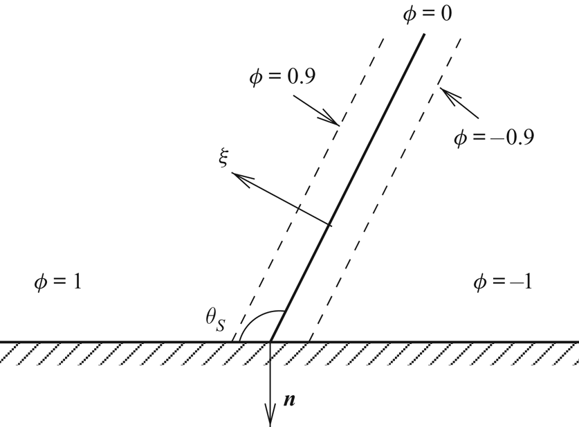
 $\phi =\pm 0.9$ contours), which guarantees the sufficient resolution of the interface (Yue et al. Reference Yue, Feng, Liu and Shen2004, Reference Yue, Zhou, Feng, Ollivier-Gooch and Hu2006). Thanks to the adaptive mesh refinement, there are only 3022 elements in the whole computational mesh corresponding to figure 4(a).
An example of the computational mesh near the drop (a) and steady-state drop shapes (b–d). The (red) dashed curve denotes the interface obtained by Schleizer & Bonnecaze (Reference Schleizer and Bonnecaze1999) using a boundary integral method. The (black) solid curves denote the  $\phi =-0.9,0,0.9$ contours by the phase-field method. Computational mesh for (a)
 $Ca=0.05$, (b)
 $Ca=0.05$, (c)
 $Ca=0.10$, (d)
 $Ca=0.15$.
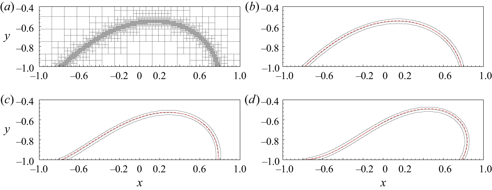
We take  ${\rm \Delta} t=0.04 ({\mu H }/{\sigma })$ and run the simulation for 1000 steps, which is sufficient for the flow to reach steady state. The numerical results are given in figure 4. For different capillary numbers, the
 $\phi =0$ level sets match the boundary integral curves very well. In theory, the contact lines should be pinned at
 $x/H=\pm 0.7814$. The contact line at the right is pinned very accurately for all
 $Ca$. In comparison, there is an observable error at the left contact line for
 $Ca=0.15$: the intersection of
 $\phi =0$ and the wall is shifted slightly downstream. This is because the contact angle is very small and the diffuse interface has a much larger intersection with the wall. This, in return, introduces more uncertainty to the exact location of the sharp interface.
5.2. Advancing and receding interfaces in plane Poiseuille flow
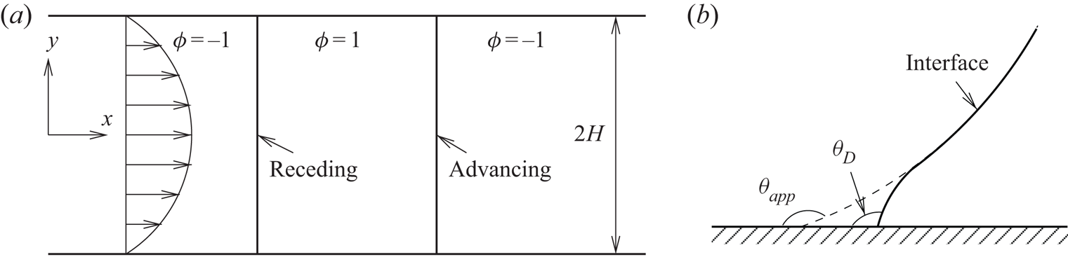
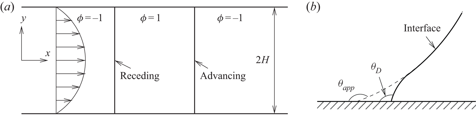
The contact lines in the previous section are pinned. In this subsection we investigate the dynamics of moving contact lines. We consider the advancing and receding interfaces between two parallel plates, as shown in figure 5(a). The velocity and stress boundary conditions are the same as those in the previous subsection. The domain size is  $10H\times 2H$. The interfaces are initially vertical lines located at
 $x=3H$ and
 $6H$. For convenience, we refer to the contact line on the left as the receding contact line and the one on the right as the advancing contact line, although they may both get pinned.
Schematic of advancing and receding interfaces under plane Poiseuille flow (a) and a zoomed-in view of the contact line (b). The dashed line in (b) represents a circular fit to the deformed interface.
We still neglect inertia and only consider matched viscosities. At steady state, the interfaces together with the contact lines move at the average velocity  $\bar V=\frac {2}{3}V_{max}$ of the Poiseuille flow. We thus define the capillary number as
 $Ca={\mu \bar V}/{\sigma }$. In the following computations, we take
 $S=0.01$,
 $\theta _A=135^{\circ }$ and
 $\theta _R=75^{\circ }$. Other parameters will be given in the detailed discussions.
The apparent contact angle is usually introduced to describe the macroscopic behaviour of the interface and there is never a unified definition that works for all flow conditions. In this work, following Hoffman (Reference Hoffman1975), we compute a circular fit to the  $\phi =0$ level set, and then determine
 $\theta _{\textit{app}}$ based on the intersection between the circular fit and the wall, as shown in figure 5(b). At small capillary numbers, the interface away from the contact line is very close to a circular arc, and
 $\theta _{\textit{app}}$ defined above faithfully represents the interface behaviour at the macroscopic length scale.
5.2.1. Transient behaviour of the contact line
We consider a small capillary number  $Ca=0.01$, under which the interfaces remain almost circular. For convenience, we define a dimensionless time
 $t^{*}=t({\bar V}/{H})$ and length
 $x^{*}={x}/{H}$.
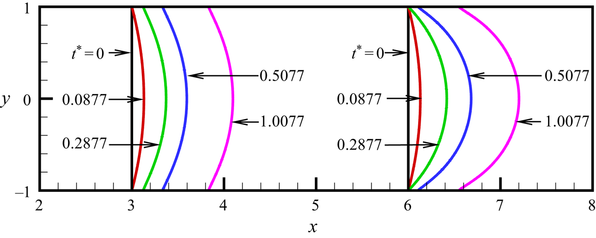
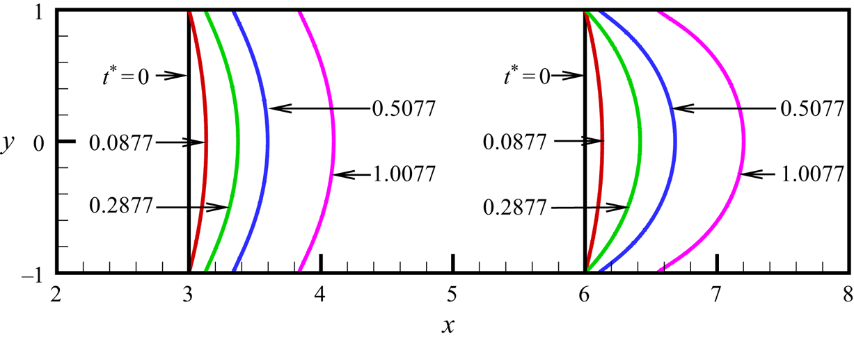
A typical interface evolution is given in figure 6. At  $t^{*}=0$, the vertical interfaces correspond to
 $\theta _D=90^{\circ }\in [\theta _R,\theta _A]$, and both contact lines are pinned. Under slow flow, each interface remains circular and
 $\theta _D=\theta _{\textit{app}}$ when the contact line is pinned. We can thus easily find out the time instant to achieve a given
 $\theta _D$ by mass conservation and geometric relations, i.e.
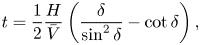 \begin{equation} t=\frac{1}{2}\frac{H}{\bar V} \left(\frac{\delta}{\sin^{2}\delta}-\cot\delta\right), \end{equation}
where  $\delta =|\frac {{\rm \pi} }{2}-\theta _D|$ is half of the central angle of the circular interface. Thus, theoretically,
 $\theta _D$ at the receding contact line achieves
 $\theta _R$ at
 $t^{*}= 0.0881$ and
 $\theta _D$ at the advancing contact line achieves
 $\theta _A$ at
 $t^{*}=0.2854$. These values agree very well with the numerical ones, which are approximately
 $t^{*}=0.0877$ and
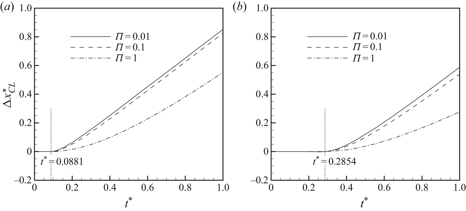
 $t^{*}=0.2877$. After these time instants the contact lines start to move, which is also manifested by figure 7.
Snapshots of advancing and receding interfaces;  $\Pi =0.1$,
 $Ca=0.01$. The dimensionless time step is set to
 ${\rm \Delta} t^{*}=10^{-4}$ initially and then gradually increases to
 $10^{-3}$. Theoretically, the receding and advancing contact lines are depinned at
 $t^{*}=0.0881$ and
 $0.2854$, respectively, if the interfaces remain circular.
Displacements of contact lines;  $Ca=0.01$. Here
 ${\rm \Delta} x^{*}_{CL}$ is the normalized
 $x$-coordinate of the contact line relative to its initial position: (a) receding contact line and (b)advancing contact line.
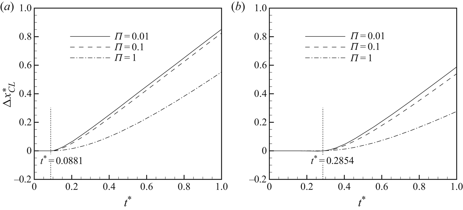
The value of  $\Pi$ affects the effective slip and thus the contact line dynamics once the contact line moves. The transient behaviours for
 $\Pi =0.01$, 0.1 and 1 are given in figures 7 and 8. It should be noted that, for each contact line, the curves for different
 $\Pi$ values collapse in the beginning. After the contact line is depinned, the effect of
 $\Pi$ kicks in and the curves start to deviate from each other.
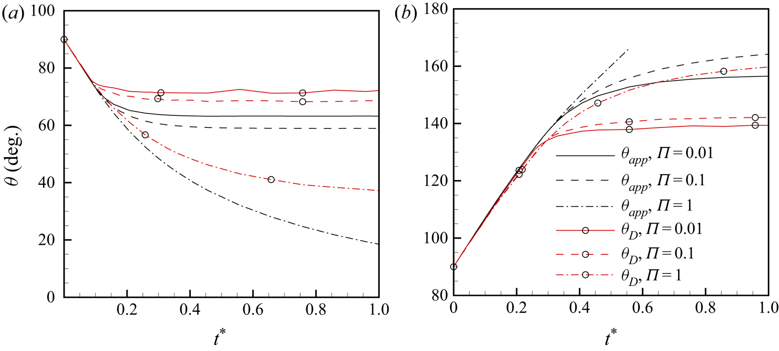
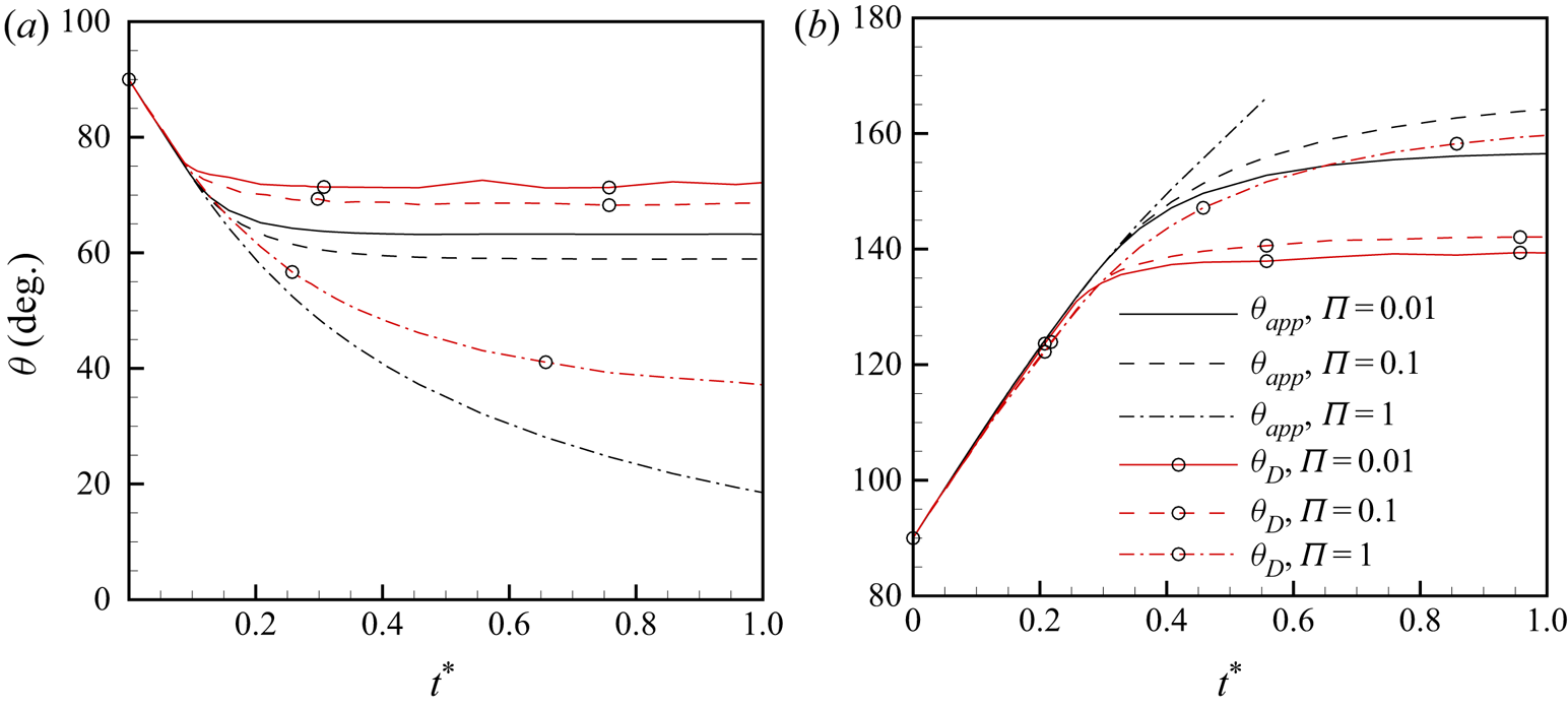
Transients of apparent and dynamic contact angles;  $Ca=0.01$: (a) receding contact line and (b) advancing contact line.
In figure 7 each contact line starts to accelerate after it is depinned and eventually achieves the steady-state contact line velocity, which equals  $\bar V$ due to mass conservation. After normalization, this velocity corresponds to a slope of 1 in figure 7. The only exception is the advancing contact line with
 $\Pi =1$, where a steady state is never achieved and wetting failure occurs. Before reaching the steady state, the contact line velocity decreases as
 $\Pi$ increases. This is easy to understand since the effective slip length decreases as
 $\Pi$ increases (Yue & Feng Reference Yue and Feng2011). In the context of the phase-field method, this trend can also be explained from energy dissipation: the dissipation rate associated with the wall energy relaxation,
 $\int _{\partial \Omega _w} \Gamma \tilde L^{2} \,{\textrm {d}}s = \int _{\partial \Omega _w} ({1}/{\Gamma }) ({\textrm {D} \phi }/{\textrm {D}t})^{2} \,{\textrm {d}}s$, is proportional to
 $\Pi \propto {1}/{\Gamma }$ for the same amount of
 ${\textrm {D} \phi }/{\textrm {D}t}$; this additional dissipation slows down the contact line motion.
The transient behaviours of contact angles are given in figure 8. The dynamic contact angle  $\theta _D$ is measured based on the
 $\phi =0$ level curve in the first two layers of cells adjacent to the wall. Compared to
 $\theta _{\textit{app}}$ from circular fitting,
 $\theta _D$ is more prone to numerical errors, as manifested by the oscillations in the
 $\theta _D$ curves with
 $\Pi =0.01$ in both figures 8(a) and 8(b). As
 $\Pi$ increases, both
 $\theta _D$ and
 $\theta _{\textit{app}}$ deviate more from the static contact angle, consistent with the analysis in Yue & Feng (Reference Yue and Feng2011). For the advancing contact line with
 $\Pi =1$, we terminate the
 $\theta _{\textit{app}}$ curve around
 $t^{*}=0.6$ because the radius of the circular fit to the interface drops below
 $H$. In this case,
 $\theta _{\textit{app}}$ exceeds
 $180^{\circ }$ and is no longer physical, which usually signifies the onset of wetting failure.
5.2.2. Steady-state contact line dynamics
From matched asymptotic analysis, Cox (Reference Cox1986) showed that, to the leading order, the apparent contact angle  $\theta _{app}$ follows
 \begin{equation} g(\theta_{app})=g(\theta_S) + Ca \ln \left(\frac{W}{l_s}\right), \end{equation}
where  $W$ is a characteristic macroscopic length,
 $l_s$ is a slip length and
 $Ca$ is the capillary number defined based on the advancing fluid. The function
 $g$ is given by
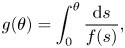 \[ g(\theta)=\int_0^{\theta} \frac{{\textrm{d}}s}{f(s)}, \]
where
 \[ f(\theta)=\frac{2 \sin\theta\{\lambda_\mu^{2}(\theta^{2}-\sin^{2}\theta)+2\lambda_\mu [\theta({\rm \pi}-\theta)+\sin^{2}\theta]+[({\rm \pi}-\theta)^{2}-\sin^{2}\theta]\}}{\lambda_\mu(\theta^{2}-\sin^{2}\theta)[({\rm \pi}-\theta)+\sin\theta\cos\theta] +[({\rm \pi}-\theta)^{2}-\sin^{2}\theta](\theta-\sin\theta\cos\theta)} \]
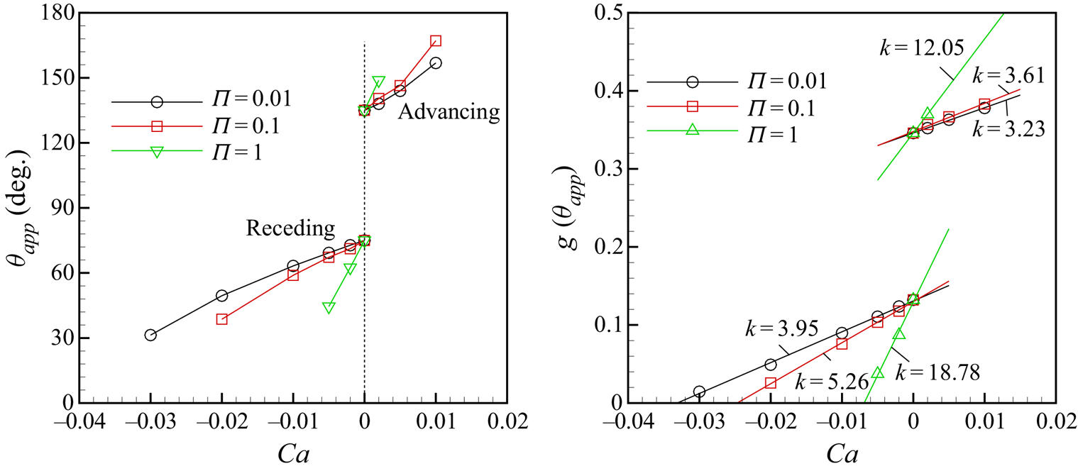
and  $\lambda _\mu$ is the viscosity ratio between the receding and advancing fluids. The steady state apparent contact angle
 $\theta _{\textit{app}}$ and the corresponding
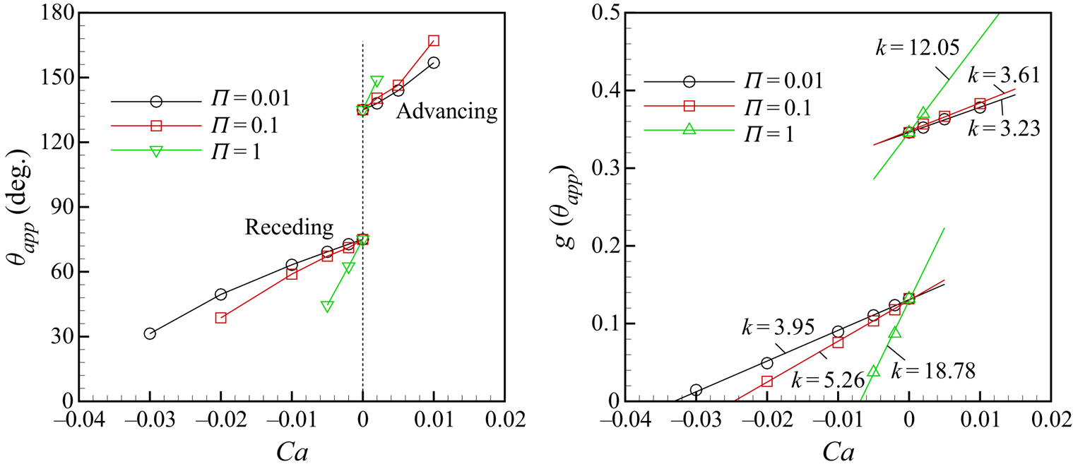
 $g(\theta _{\textit{app}})$ from phase-field simulations are given in figure 9, where the linear relation between
 $g(\theta _{\textit{app}})$ and
 $Ca$ is faithfully captured for both the advancing and receding contact lines at different
 $\Pi$ values.
Steady-state dynamics of moving contact lines:  $\theta _R=75^{\circ }$,
 $\theta _A=135^{\circ }$,
 $\lambda _\mu =1$,
 $S=0.01$,
 $Cn=0.01$. The contact line advances if
 $Ca>0$ and recedes if
 $Ca<0$. The
 $k$ values are the slopes of linear fits.
According to Yue et al. (Reference Yue, Zhou and Feng2010), the slip length of the phase-field model due to interfacial mobility is approximately  $2.5l_D$ for fluids with equal density. Furthermore, good agreements between Cox's formula and the phase-field method are achieved when
 $W$ is taken to be the radius of the pipe for Poiseuille flows. For the plane Poiseuille flow considered here, it is then reasonable to take
 $W$ to be the half-channel height
 $H$. When wall energy relaxation exists, the actual slip
 $l_s$ differs from the
 $2.5l_D$. According to Yue & Feng (Reference Yue and Feng2011), we have
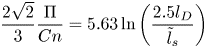 \begin{equation} \frac{2\sqrt 2}{3}\frac{\Pi}{Cn} = 5.63 \ln \left(\frac{2.5 l_D}{\tilde l_s}\right) \end{equation}
for  $\theta _D$ close to
 $90^{\circ }$. Thus, the slope of the
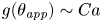 $g(\theta _{\textit{app}})\sim Ca$ curve should be
 \[ k=\ln\left(\frac{W}{l_s}\right)= \ln\left(\frac{H}{2.5 l_D}\right) + \ln \left(\frac{2.5 l_D}{\tilde l_s}\right)= \ln\left(\frac{1}{2.5 S}\right)+ \frac{2\sqrt 2}{3}\frac{\Pi}{5.63 Cn}. \]
This gives the theoretical slopes of  $k=3.86$,
 $5.36$ and
 $20.44$ for
 $\Pi =0.01$, 0.1 and 1, respectively. These values agree reasonably well with the numerical values for the receding contact lines in figure 9(b). Much greater discrepancies are however observed on the advancing branch. This is probably because
 $\theta _D$ is too close to
 $180^{\circ }$. In this case, (5.6) is less accurate and we also expect larger errors in computing
 $\theta _{\textit{app}}$.
In summary, our current method captures the correct contact line dynamics, similar to the standard phase-field method without CAH (Yue et al. Reference Yue, Zhou and Feng2010; Yue & Feng Reference Yue and Feng2011). The only complication is that  $\theta _S$ may take different values, i.e.
 $\theta _R$ or
 $\theta _A$, depending on whether the contact line recedes or advances.
5.2.3. Pinning of the contact line and choice of $\Gamma$

As we have mentioned before, the discretized weak form can not guarantee the exact satisfaction of (3.3). That is, in real calculations, the contact line may still move even when it is supposed to be pinned. This actually happens when  $\Pi$ (or
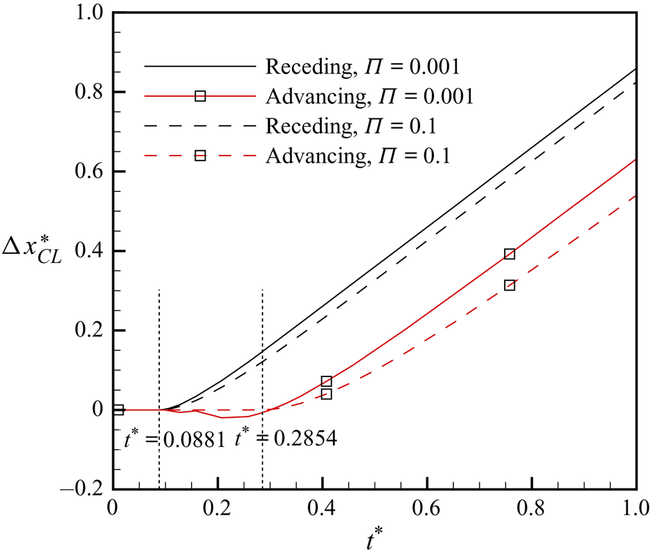
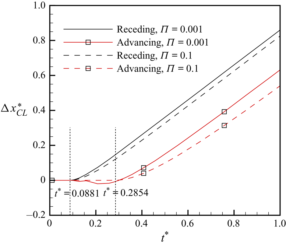
 ${1}/{\Gamma }$) is not sufficiently large, as shown in figures 10 and 11(b). The advancing contact line with
 $\Pi =0.001$ recedes slightly when it is supposed to be pinned at
 $t^{*}<0.2854$. At
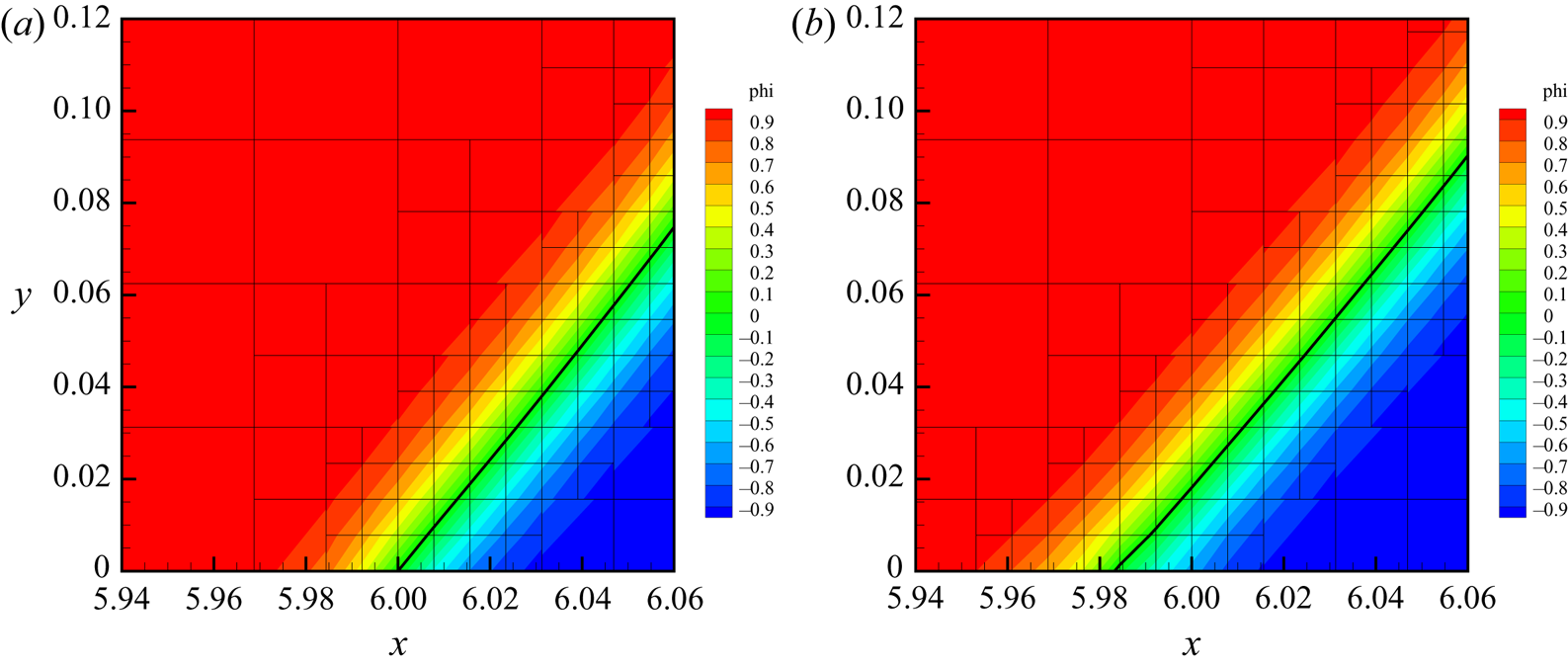
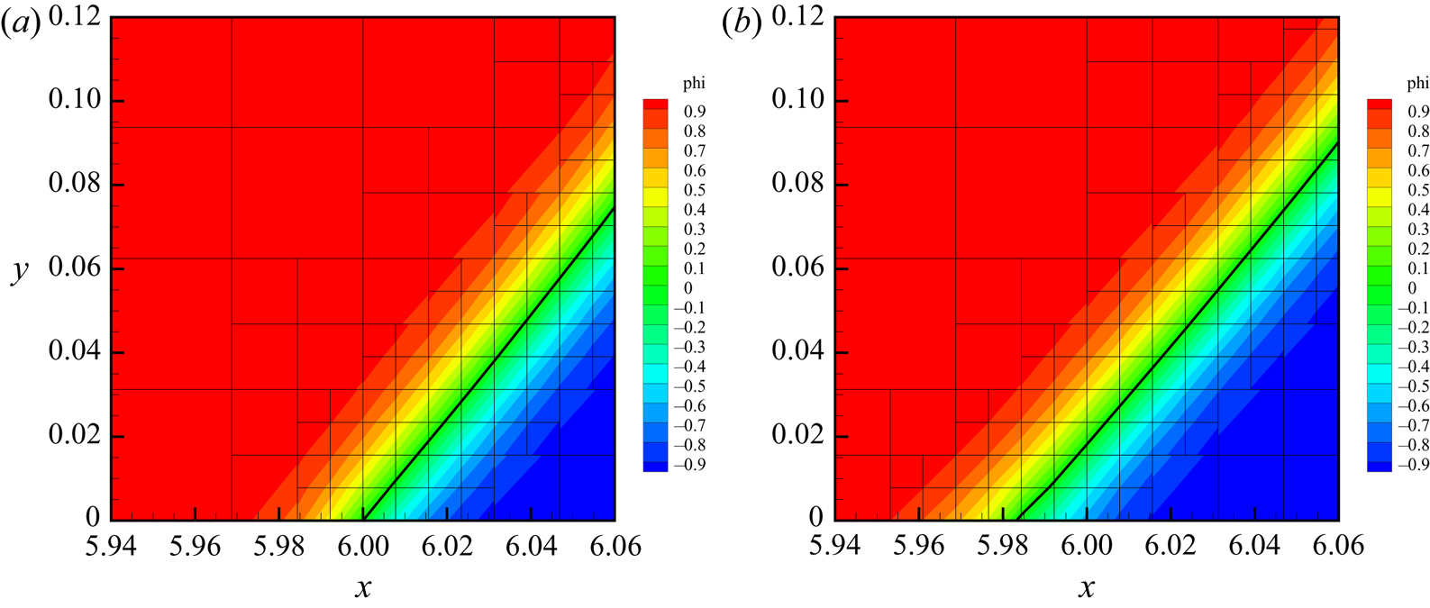
 $t^{*}=0.2577$, the contact line with
 $\Pi =0.1$ is nicely pinned at
 $x^{*}=6$ while that with
 $\Pi =0.001$ shifts upstream by about two grid cells. A close inspection of figure 11(b) shows that the diffuse interface is slightly dilated near the wall. This type of pinning failure does not happen to the receding contact line, where the dynamic contact angle is very close to
 $90^{\circ }$ before the contact line moves. Numerical tests with various contact angles and
 $\Pi$ reveal that the pinning failure is more likely to occur for a smaller
 $\Pi$ and when
 $\theta _D$ is further away from
 $90^{\circ }$.
Pinning failure at a small  $\Pi$;
 $\theta _R=75^{\circ }$,
 $\theta _A=135^{\circ }$,
 $Ca=0.01$,
 $S=0.01$,
 $Cn=0.01$.
Plots of the  $\phi$ contours at the vicinity of the advancing contact line at
 $t^{*}=0.2577$;
 $\theta _R=75^{\circ }$,
 $\theta _A=135^{\circ }$,
 $Ca=0.01$,
 $S=0.01$,
 $Cn=0.01$. (a)
 $\Pi =0.1$, (b)
 $\Pi =0.001$. The thick lines denote the interface (
 $\phi =0$) and the thin lines are grid lines. The contact line is supposed to be pinned at
 $x^{*}=6$.
To capture contact line pinning with good accuracy, we need a guideline for the choice of  $\Pi$, i.e.
 $\Gamma$. By inspecting (4.12), we note that the energy dissipation rate on the solid wall
 $\partial \Omega _w$ for a pinned contact line can be written as
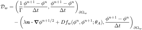 \begin{align} {\mathcal{D}}_w&=\left(\frac{1}{\Gamma}\frac{\phi^{{n+1}}-\phi^{n}}{{\rm \Delta} t},\frac{\phi^{{n+1}}-\phi^{n}}{{\rm \Delta} t}\right)_{\partial\Omega_w}\nonumber\\ &\quad -\left(\lambda\boldsymbol{n}\boldsymbol{\cdot} \boldsymbol{\nabla}\phi^{{n+{1}/{2}}} + Df_w(\phi^{n},\phi^{{n+1}};\theta_A), \frac{\phi^{{n+1}}-\phi^{n}}{{\rm \Delta} t}\right)_{\partial\Omega_w} \end{align}
and is supposed to be zero since  $\phi ^{{n+1}}=\phi ^{n}$. However, in practice,
 $\phi ^{{n+1}}=\phi ^{n}$ is not guaranteed by the weak form and we have no control over the sign of the second term of
 ${\mathcal {D}}_w$. A negative dissipation
 ${\mathcal {D}}_w<0$ may thus occur and lead to numerical instability. A positive dissipation can be achieved if the first term overpowers the second term, which can be roughly satisfied by
 $|({1}/{\Gamma })({\partial \phi }/{\partial t})| \gtrsim | \lambda \boldsymbol {n}\boldsymbol {\cdot } \boldsymbol {\nabla }\phi |$. For a contact line moving with speed
 $V$ and angle
 $\theta _D$, we have
 $|{\partial \phi }/{\partial t}| \sim V |\boldsymbol {\nabla }\phi | |\sin \theta _D|$ and
 $|\lambda \boldsymbol {n}\boldsymbol {\cdot } \boldsymbol {\nabla }\phi | \sim \sigma \epsilon |\boldsymbol {\nabla }\phi | |\cos \theta _D|$. This leads to the approximate criterion
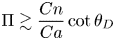 \begin{equation} \Pi \gtrsim \frac{Cn}{Ca} \cot\theta_D \end{equation}
for numerical stability.
We have tested different combinations of  $\Pi$,
 $Ca$,
 $Cn$ and
 $S$, with
 $\theta _R=75^{\circ }$ and
 $\theta _A=135^{\circ }$ being fixed. For the advancing contact line to falsely recede for the same displacement,
 $\Pi$ has to be chosen such that it is proportional to
 $Cn$, inversely proportional to
 $Ca$ and independent of
 $S$, i.e.
 $\Pi \propto {Cn}/{Ca}$.
To investigate the influence of  $\theta _D$, we take
 $\theta _A=170^{\circ }$ so that pinning failure eventually occurs when
 $\theta _D$ is sufficiently close to
 $180^{\circ }$. We compute the advancing contact line with
 $\Pi =0.001$, 0.01, 0.1, 0.2 and 0.5, until the contact line starts to move upstream for about one grid spacing
 $h_{min}$. Other parameters are kept constant:
 $Ca=0.01$,
 $S=0.01$ and
 $Cn=0.01$. The instantaneous
 $\theta _D$ is then recorded as the critical value that causes pinning failure. We have also tested
 $\Pi =1$, but pinning failure never occurs. The numerical results, however, do not suggest a linear relation between the
 $\Pi$ and
 $\cot \theta _D$. If we relax (5.8) to
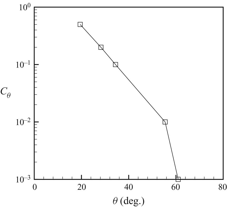
 \begin{equation} \Pi \gtrsim \frac{Cn}{Ca} C_\theta \end{equation}
then parameter  $C_\theta$ can be numerically determined as shown in figure 12.
Numerical values of  $C_\theta$.
 $\theta =\min (\theta _D,{\rm \pi} -\theta _D)$.
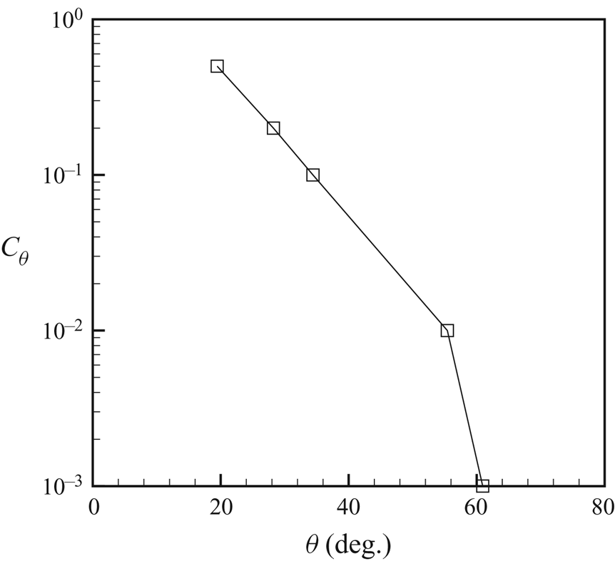
To achieve desired pinning performance in practical computations, we suggest using (5.9) together with figure 12 as a guideline for choosing  $\Pi$. It should be noted that the derivations and numerical tests here are by no means rigorous.
5.2.4. A computational strategy for hysteresis
In the absence of CAH, a computational strategy has been proposed in Yue & Feng (Reference Yue and Feng2011) as follows. First, we choose a capillary width  $\epsilon$ (or the dimensionless group
 $Cn$) based on the computational mesh that we can afford. Usually, we take
 $\epsilon \in [h_{min}, 2 h_{min}]$, where
 $h_{min}$ is the mesh size at the interface. This guarantees that the diffuse interface is sufficiently resolved. To reduce the influence of interfacial thickness on numerical results,
 $Cn$ should be as small as possible, e.g.
 $Cn\le 0.01$, which makes adaptive mesh refinement almost necessary. Second, we choose the mobility parameter
 $M$ such that the diffusion length is well resolved:
 $l_D=\sqrt {M\mu }>\epsilon /4$ (or
 $S\ge Cn/4$ in the dimensionless form). This guarantees that the numerical results are independent of
 $\epsilon$ and
 $h_{min}$. Finally, we tune
 $\Gamma$ (or the dimensionless group
 $\Pi$) to achieve the desired effective slip length.
This last step may however lead to a  $\Pi$ that is too small to numerically pin the contact line. Actually, the wall energy relaxation parameter
 $\Gamma$ has no physical meaning when the contact line is pinned and we just need a non-zero number. Furthermore, there is no physical requirement that
 $\Gamma$ must be a single-valued constant. We thus allow
 $\Gamma$ to take different values depending on the status of the contact line and amend the third step above as follows. We estimate a
 $\Gamma$ for pinning, denoted by
 $\Gamma _P$, based on (5.9) or numerical experiments. If
 $\Gamma$ required for slip is greater than
 $\Gamma _P$ then we impose
 $\Gamma _P$ where the contact line is pinned and
 $\Gamma$ elsewhere.
5.3. Oscillating drop
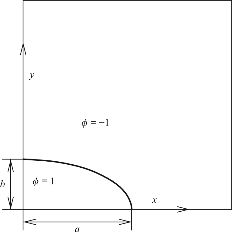
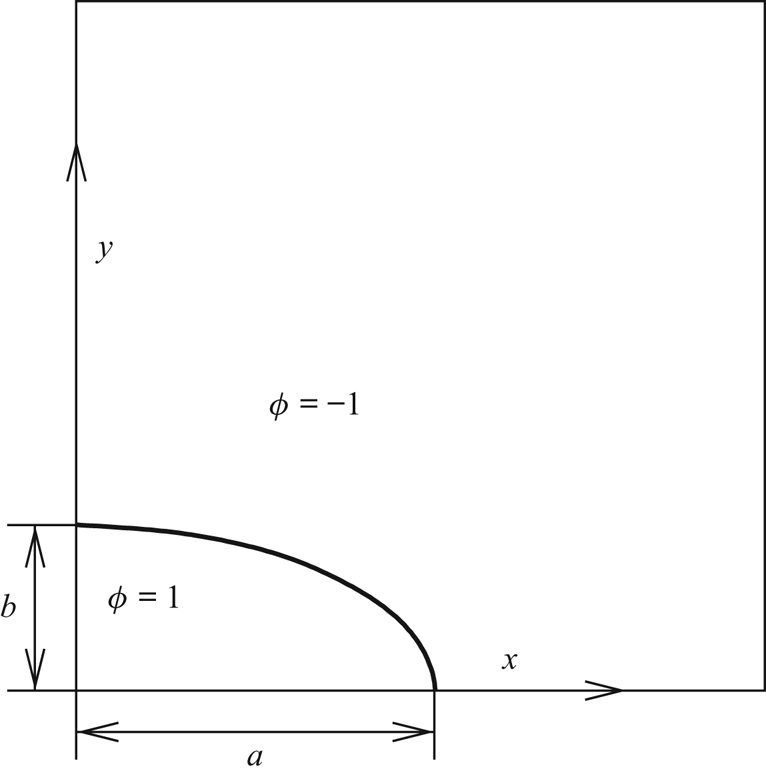
In this subsection we consider an oscillating drop on a solid wall, where the contact line transitions between receding, pinning and advancing. A schematic of the computational set-up is given in figure 13. The initially elliptic drop will undergo oscillations due to inertia-capillary effects. The computational domain is a square of  $4R_0\times 4R_0$. Symmetry conditions are applied at the two vertical boundaries. Zero traction is applied on the upper boundary. The lower boundary is a solid wall with no-slip velocity and prescribed contact line conditions.
Schematic of an oscillating drop. The drop is initially elliptic with semi-axes  $a=2R_0$ and
 $b=0.5R_0$, where
 $R_0$ is the effective drop radius.
For convenience, we use effective drop radius  $R_0$, drop density
 $\rho _1$ and surface tension
 $\sigma$ to non-dimensionalize all the parameters, and denote the dimensionless parameters with a superscript
 $^{*}$. For example,
 $t^{*}=t/t_c$, where
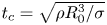 $t_c=\sqrt {{\rho R_0^{3}}/{\sigma }}$ is the capillary time, viscosity
 $\mu ^{*}={\mu }/{\sqrt {\rho _1\sigma R_0}}$ and energy
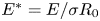 $E^{*}={E}/{\sigma R_0}$.
The fluid parameters are  $\rho _1^{*}=1$,
 $\rho _2^{*}=0.01$,
 $\mu _1^{*}=0.01$,
 $\mu _2^{*}=0.001$ and
 $\sigma ^{*}=1$. This choice corresponds to a small Ohnesorge number
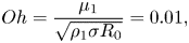 \begin{equation} Oh=\frac{\mu_1}{\sqrt{\rho_1\sigma R_0}}=0.01, \end{equation}
such that the oscillation is not overdamped. For the diffuse interface, we choose  $\epsilon ^{*}=0.01$,
 $M^{*}=10^{-3}$ and
 $\Gamma ^{*}=10^{3}$. Some relevant dimensionless groups are
 $S={\sqrt {M \mu _1}}/{R_0}=3.16\times 10^{-3}$ and
 $\Pi ={1}/{\mu _1\Gamma R_0} = 0.1$. For the computational mesh, we choose
 $h_{min}^{*}=\frac {1}{128}$ at the interface and
 $h_{max}^{*}=\frac {1}{4}$ in the bulk.
We run three simulations with different contact angles:  $(\theta _R, \theta _A)=(90^{\circ },90^{\circ })$,
 $(90^{\circ }, 105^{\circ })$,
 $(75^{\circ }, 105^{\circ })$. The evolution of the drop interface for
 $(90^{\circ }, 105^{\circ })$ and
 $(90^{\circ }, 90^{\circ })$ are shown in figures 14 and 15, respectively. In the initial stage, the contact line moves to the left (i.e. recedes), and its dynamics is controlled by
 $\theta _R$ solely. Therefore, these two cases are identical before the contact line stops at the leftmost position at
 $t^{*}\approx 1.723$. This is also manifested by the overlapping curves at
 $t^{*}\lesssim 1.723$ in figures 16 and 17. For
 $(\theta _R, \theta _A)=(90^{\circ },105^{\circ })$, the contact line is pinned for a short period (around
 $t\in [1.723,1.960]$) while the interface continues to protrude to the right. Once
 $\theta _D$ reaches
 $105^{\circ }$ (
 $t\approx 1.960$), the contact line starts to move rightward. The contact line is pinned again around
 $t\in [3.073,3.0534]$, and then retracts. Finally, the contact line stays pinned after
 $t^{*}=4.033$ while the other part of the interface keeps oscillating. In contrast, there is no obvious contact line pinning for
 $(\theta _R, \theta _A)=(90^{\circ },90^{\circ })$, i.e. when there is no CAH.
Snapshots of an oscillating drop with CAH;  $\theta _R=90^{\circ }$,
 $\theta _A=105^{\circ }$. The contact line is pinned at
 $t^{*}\in [1.723,1.960]$,
 $[3.073,3.534]$ and
 $[4.033,\infty )$.
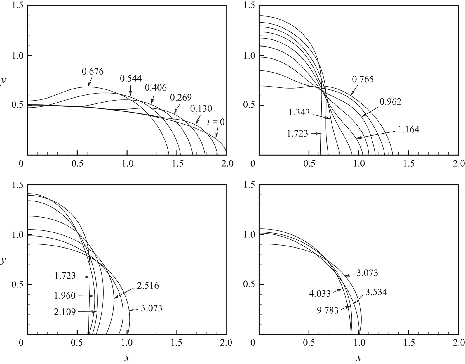
Snapshots of an oscillating drop without CAH;  $\theta _R=\theta _A=90^{\circ }$.
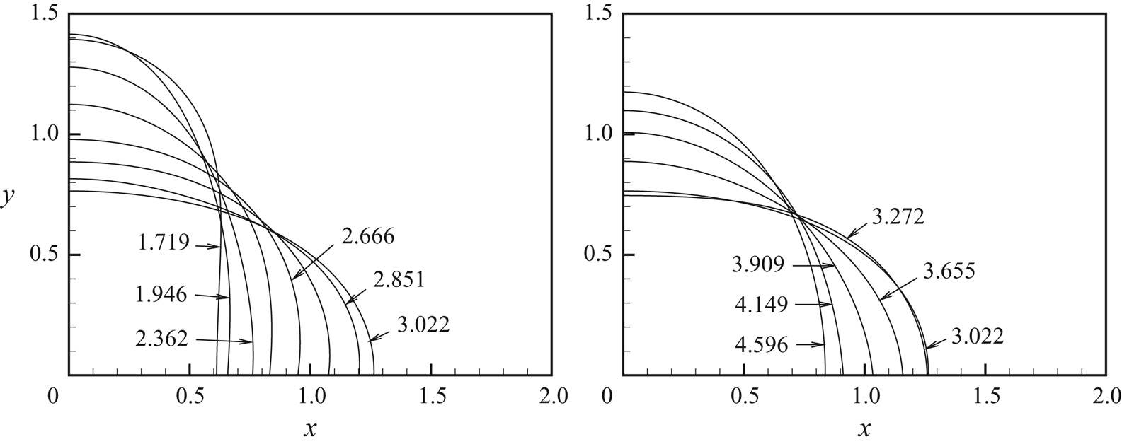
Contact line positions of oscillating drops. The plateaus denote the pinning of contact lines.
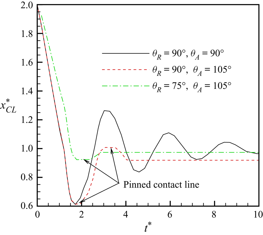
Time history of dimensionless free energies of oscillating drops: (a) kinetic energy, (b) mixing energy, (c) total energy excluding wall energy and (d) total energy.
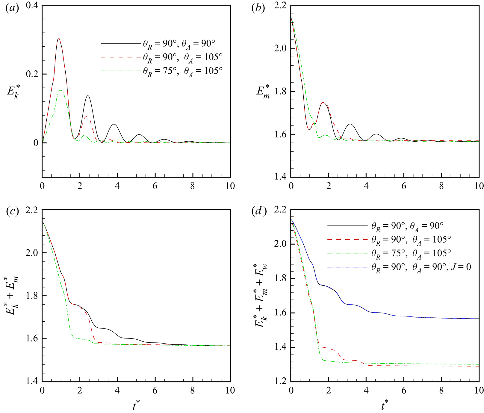
At  $t^{*}\to \infty$, the drop will eventually settle to a static circular shape. The contact line position, i.e. the spreading radius, is related to the
 $\theta _{\textit{app}}$ (which is also the same as
 $\theta _D$) by
 \[ x_{CL}^{*}=\sqrt{\frac{{\rm \pi}}{2[\theta_{\mathit{app}} -\frac{1}{2}\sin(2\theta_{\mathit{app}})]}}\sin\theta_{\mathit{app}}. \]
This gives  $x_{CL}^{*}=1.176$,
 $1$ and
 $0.839$ for
 $\theta _{\textit{app}}=75^{\circ }$,
 $90^{\circ }$ and
 $105^{\circ }$, respectively. The trajectories of the contact line are given in figure 16. It is obvious that the contact line keeps oscillating around
 $x_{CL}^{*}=1$ when there is no CAH. When there exists CAH, the contact line is finally pinned at
 $x_{CL}^{*}=0.919$ and 0.973 for
 $(\theta _R, \theta _A)=(90^{\circ }, 105^{\circ })$ and
 $(75^{\circ }, 105^{\circ })$, both in the range determined by
 $\theta _R$ and
 $\theta _A$. But the exact location of the final
 $x_{CL}^{*}$ is also dependent on the transient process, i.e. the history of the contact line.
The evolution of free energies are given in figure 17. Here, the dimensionless free energies are computed as follows: kinetic energy  $E_k^{*}={\int _{\Omega }\frac {1}{2}\rho |\boldsymbol {u}|^{2}\,{\textrm {d}}\boldsymbol {x}}/({\sigma R_0})$, mixing energy
 $E_m^{*}={\int _{\Omega }f_m\,{\textrm {d}}\boldsymbol {x}}/({\sigma R_0})$ and wall energy
 $E_w^{*}={\int _{\partial \Omega _w}f_w(\phi ;\theta _A) \,{\textrm {d}}s}/({\sigma R_0})$. At
 $t^{*}=0$, the whole system is static, which corresponds to a zero kinetic energy
 $E^{*}_k$ and a maximum mixing energy
 $E^{*}_m$. As the drop retracts, part of the mixing energy is converted into kinetic energy. The repeated conversions between mixing and kinetic energies are manifested by the oscillatory curves in figures 17(a) and 17(b). As time approaches
 $t^{*}=10$,
 $E_k^{*}$ drops to zero while
 $E_m^{*}$ stabilizes around 1.57. The latter is consistent with the surface energy of a drop with
 $\theta _{\textit{app}}=90^{\circ }$:
 $({{\rm \pi} }/{2})\sigma R_0^{2} =1.571\sigma R_0^{2}$. The two curves with CAH stabilize much faster than the one without due to additional dissipation from CAH.
In the initial retraction stage ( $t^{*}\lesssim 1.723$), the
 $E_k^{*}$ curve for
 $\theta _R=75^{\circ }$ deviates from the other two because contact line dynamics is determined by
 $\theta _R$. Similarly, the sum
 $E_k^{*}+E_m^{*}$ decreases faster for
 $\theta _R=75^{\circ }$ in the initial retraction stage, as shown in figure 17(c). The evolution of the total free energy is provided in figure 17(d) to demonstrate the energy dissipative nature of our model. Although we can only prove the discrete energy law (4.12) for matched density and zero CAH, the numerical solutions satisfy a dissipative discrete energy law for a broader choice of parameters.
We also investigate the influence of the diffusive flux  $\boldsymbol{J}$ on the phase-field simulations of interfacial flows with non-matched densities. We set
 $\boldsymbol{J}=0$, i.e. neglecting the diffusive flux as in many previous phase-field simulations (e.g. Jacqmin Reference Jacqmin1999; Villanueva & Amberg Reference Villanueva and Amberg2006; Yue et al. Reference Yue, Zhou, Feng, Ollivier-Gooch and Hu2006; Khatavkar et al. Reference Khatavkar, Anderson, Duineveld and Meijer2007a), and show the result for
 $\theta _R=\theta _A=90^{\circ }$ in figure 17(d). The curve with
 $\boldsymbol{J}=0$ is almost identical to the one considering diffusive flux. This is not surprising because the diffusive flux only occurs in the diffuse-interface region and its effect diminishes as
 $Cn$ decreases. Thus, in interfacial flows with non-matched densities we expect the diffusive flux
 $\boldsymbol{J}$ to be negligible, at least in the case of
 $Cn\ll 1$.
5.4. Three-dimensional drop on an inclined wall
Our code can be easily switched to three dimensions, thanks to the dimension-independent programming advocated in deal.ii (Bangerth Reference Bangerth2000). However, the discrete system resulting from the mixed finite element method is very costly to solve and thus we can only perform some preliminary 3-D simulations. A more efficient projection-based flow solver is currently under development. The purpose of this subsection is only to demonstrate the capability of our hysteresis model in 3-D flows.
We consider a drop on an inclined wall, as shown in figures 18 and 19. Similar to § 5.3, we use drop density  $\rho _1$, surface tension
 $\sigma$ and drop radius
 $R_0$ to non-dimensionalize all parameters. Owing to symmetry in the
 $z$-direction, we only compute half of the drop. The computational domain is a rectangular box defined by
 $[0,8]\times [0,3]\times [0,3]$ with a hemispherical drop initially centred at
 $(5,0,0)$. The following dimensionless parameters are adopted:
 $\rho _1^{*}=1$,
 $\rho _2^{*}=0.01$,
 $\mu _1^{*}=1$,
 $\mu _2^{*}=0.01$,
 $\sigma ^{*}=1$,
 $R_0^{*}=1$,
 $\epsilon ^{*}=0.02$,
 $M^{*}=10^{-4}$,
 $\theta _R=60^{\circ }$,
 $\theta _A=120^{\circ }$,
 $\Gamma ^{*}=100$ and slope inclination angle
 $\alpha =60^{\circ }$. These parameters correspond to the following dimensionless groups:
 $Cn={\epsilon }/{R_0}=\epsilon ^{*}=0.02$,
 $S={\sqrt {M\mu _1}}/{R_0}=\sqrt {M^{*}}=10^{-2}$,
 $\Pi ={1}/{\mu _1\Gamma R_0}= {1}/{\Gamma ^{*}}=0.01$ and
 $Oh={\mu _1}/{\sqrt {\rho _1\sigma R_0}}=1$. We test
 $g^{*}=1$ and
 $g^{*}=2$, which correspond to the Bond numbers
 $Bo={(\rho _1-\rho _2)gR_0^{2}}/{\sigma }=(1-\rho _2^{*})g^{*}=0.99$ and 1.98, respectively. For the computational mesh, we choose
 $h^{*}_{min}=\frac {1}{64}$ at the interface and
 $h^{*}_{max}=\frac {1}{8}$ in the bulk. The time step is set to
 ${\rm \Delta} t^{*}=0.01$ initially and is gradually increased to
 ${\rm \Delta} t^{*}=0.05$.
Three-dimensional drop sticking to an inclined wall;  $Bo=0.99$: (a)
 $t^{*}=0$, (b)
 $t^{*}=4.52$ and (c)
 $t^{*}=24.52$.
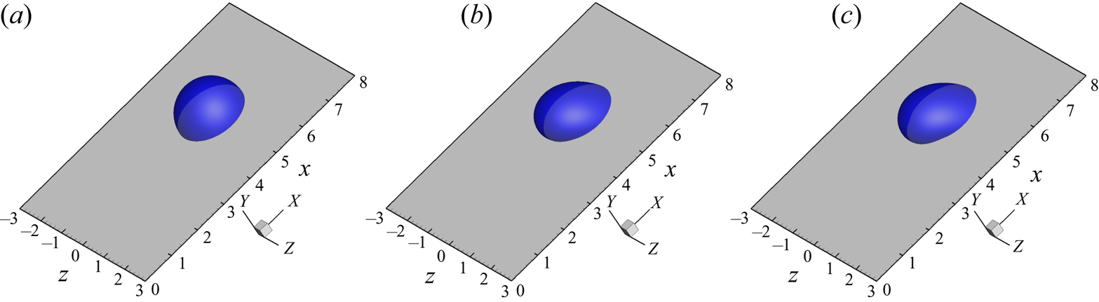
Three-dimensional drop sliding on an inclined wall;  $Bo=1.98$: (a)
 $t^{*}=0$, (b)
 $t^{*}=4.52$, (c)
 $t^{*}=14.52$, (d)
 $t^{*}=24.52$, (e)
 $t^{*}=34.52$ and (f)
 $t^{*}=44.52$.
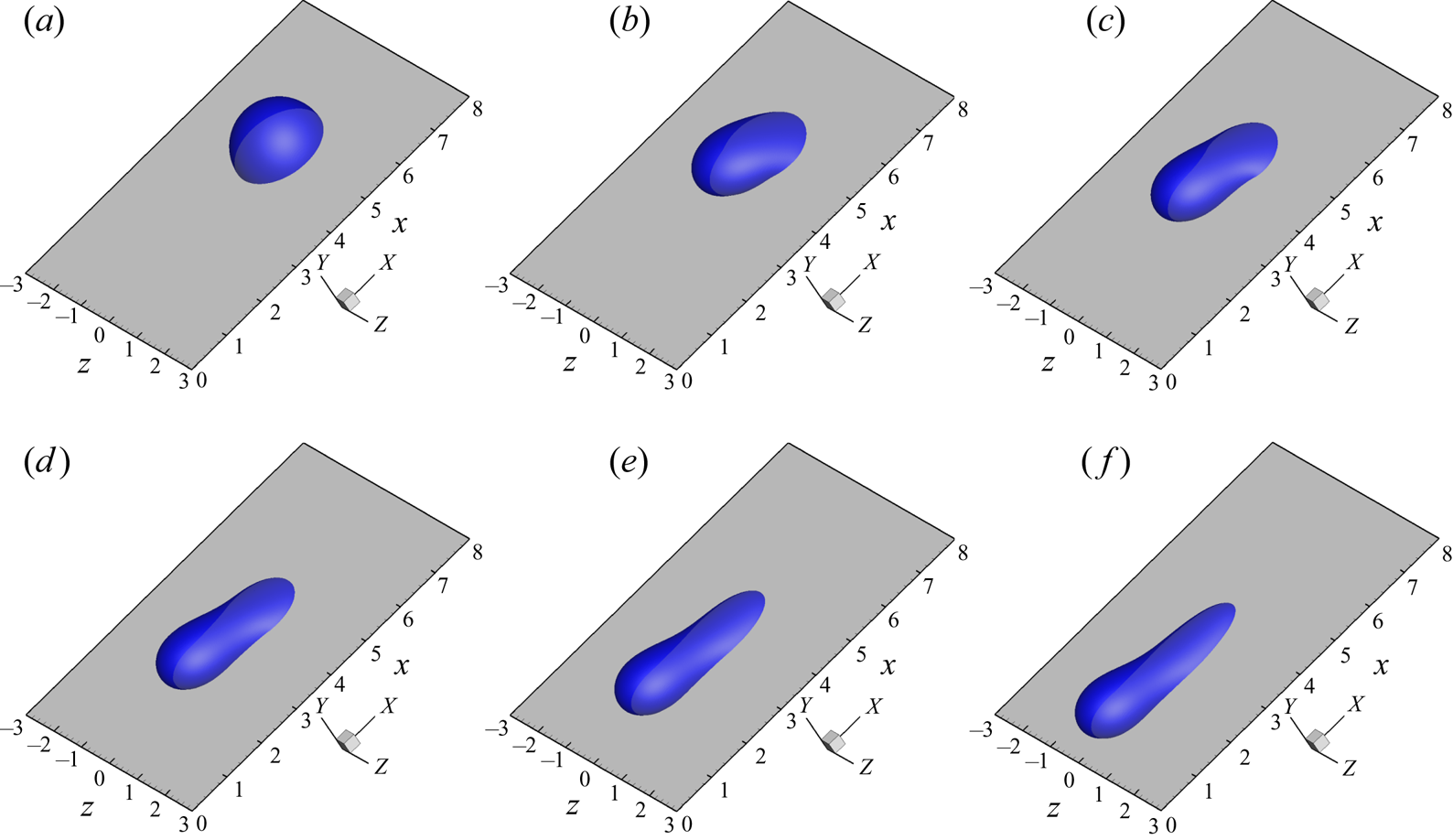
To achieve a good pinning performance, we take a smaller wall energy relaxation parameter  $\Gamma _P^{*}=10$ (such that
 $\Pi _P=0.1$) when the contact line is pinned. It should be noted that this problem does not have a well-defined capillary number when the drop is pinned as shown in figure 18. In this case, we can do a rough estimation. Suppose we want the pinned contact line to move less than the grid spacing
 $h^{*}_{min}$ during the whole simulation that lasts for
 $t^{*}\sim 20$. This gives
 $Ca\sim 10^{-3}$ and then (5.9) predicts
 $\Pi \gtrsim 0.02$ if we take
 $C_\theta =0.001$ based on figure 12. Thus,
 $\Pi _P=0.1$ should be a safe choice.
It is well known that, due to CAH, relatively small drops have a tendency to stick to solid surfaces even when the latter is tilted. The critical parameters for the onset of drop sliding satisfy
 \begin{equation} (\rho_1-\rho_2)V_d g\sin\alpha=w\sigma (\cos\theta_R-\cos\theta_A), \end{equation}
where  $V_d$ is the volume of the drop and
 $w$ is the width of the drop. This relation was first given by Furmidge (Reference Furmidge1962) based on experimental observations, and was later proved to be exact by Dussan V. & Chow (Reference Dussan V. and Chow1983) as long as the footprint of the drop is convex. In practice,
 $w$ is dependent on drop deformation and is unknown a priori. However, for an initially hemispherical drop, we can take the approximation
 $w\approx 2R_0$. This leads to the critical Bond number
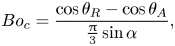 \begin{equation} Bo_c=\frac{\cos\theta_R-\cos\theta_A}{\frac{{\rm \pi}}{3}\sin\alpha}, \end{equation}
which is 1.1027 for our chosen angles. It should be noted that  $Bo_c$ in the real situation may be more complicated and a problem-dependent prefactor needs to be included (Janardan & Panchagnula Reference Janardan and Panchagnula2014).
Theoretically, the drop with  $Bo=0.99$ should stick to the slope while the drop with
 $Bo=1.98$ should slide. This is confirmed by our numerical results in figures 18 and 19. The side views of the drops are given in figure 20, where the initial pinning of the contact line is observed for both Bond numbers. It should be noted that the contact line in (a) moves slightly because of the initial transient and the fact that
 $Bo=0.99$ is very close to the critical value. The top views of the drops, i.e. the contact lines, are given in figure 21. Theoretically, we expect a steadily sliding drop to have two straight sides parallel to the moving direction (Furmidge Reference Furmidge1962; Eral et al. Reference Eral, ’t Mannetje and Oh2013). This trend can be found from the contact line shape at
 $t^{*}=44.52$. It should be noted that we have to terminate the simulation before a steady state was achieved because of the small computational domain. We will leave computations with realistic fluid properties and a larger computational domain for future work when a much more efficient flow solver is ready.
Side views of 3-D drops on an inclined wall: (a)  $Bo=0.99$ and (b)
 $Bo=1.98$.
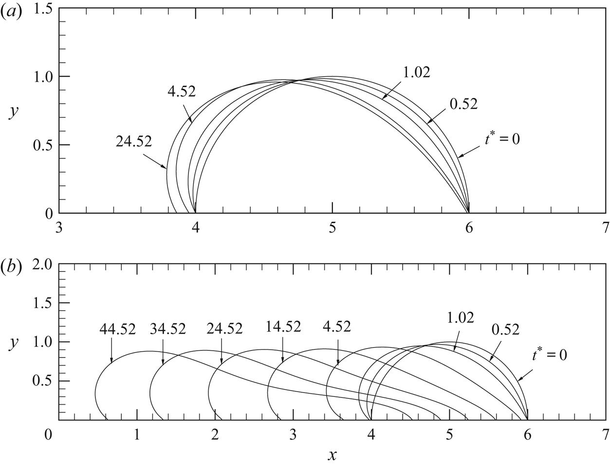
Evolution of contact lines: (a)  $Bo=0.99$ and (b)
 $Bo=1.98$.
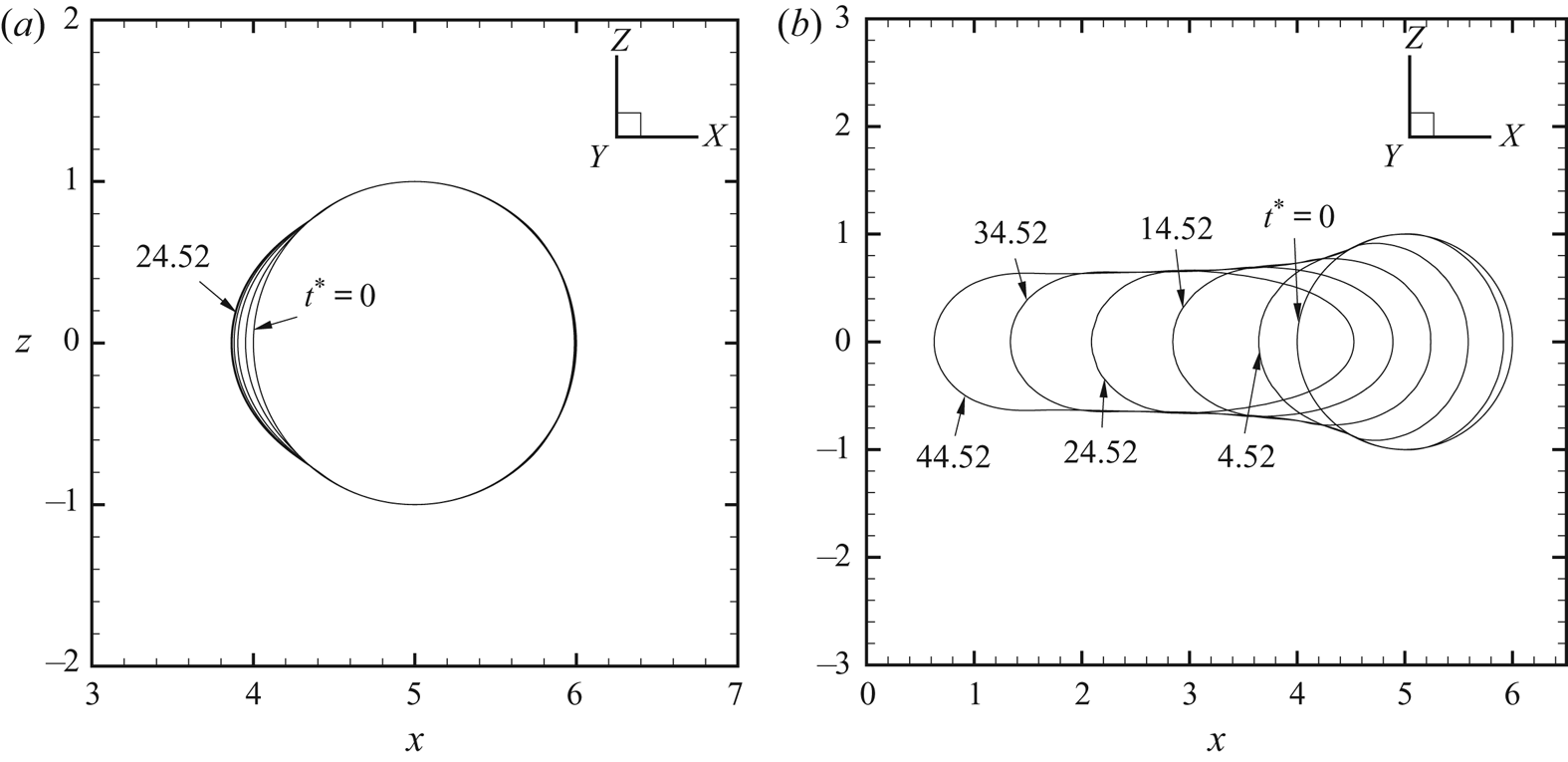
In the end we investigate the dynamic contact angle  $\theta _D$. It is difficult to directly measure
 $\theta _D$ based on the level surface of
 $\phi =0$ in three dimensions. We thus compute
 $\theta _D$ based on the relation
 $\cos \theta _D= ({\boldsymbol {n} \boldsymbol {\cdot } \boldsymbol {\nabla }\phi })/{|\boldsymbol {\nabla }\phi |}$ and the results are shown in figure 22. For the static drop in (a),
 $\theta _D\in [60^{\circ },120^{\circ }]$ along the whole contact line, consistent with the pinning condition. For the sliding drop in (b),
 $\theta _D>120^{\circ }$ at the leading edge,
 $\theta _D<160^{\circ }$ at the trailing edge and
 $\theta _D\in [60^{\circ },120^{\circ }]$ along majority of the two sides. Correspondingly, the contact line advances at the leading edge, recedes at the trailing edge and is pinned at the two sides as expected.
Dynamic contact angle: (a)  $Bo=0.99$,
 $t^{*}=24.52$ and (b)
 $Bo=1.98$,
 $t^{*}=44.52$.
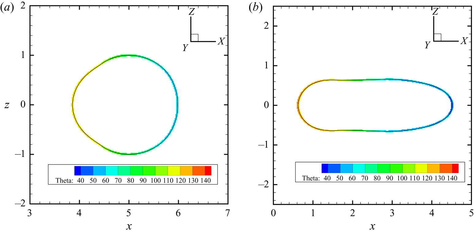
6. Concluding remarks
We have developed an energy-based boundary condition for CAH. The wall energy relaxation allows the two-phase system to deviate from equilibrium at the contact line. As a result, the microscopic dynamic contact angle  $\theta _D$, which is computed by the phase-field method, may differ from the prescribed static angle
 $\theta _S$. The tendency of contact line motion can then be deduced from the difference between these two angles. When CAH exists, the single valued
 $\theta _S$ is extended to a range of angles, namely, the hysteresis window
 $[\theta _R,\theta _A]$. Similarly, the tendency of contact line motion can be readily obtained from the computed
 $\theta _D$ and the prescribed
 $\theta _R$ and
 $\theta _A$: the contact line advances if
 $\theta _D>\theta _A$, recedes if
 $\theta _D<\theta _R$ and is pinned otherwise. The major conclusions are summarized as follows.
(i) In the phase-field method the relations between
$\theta _D$, $\theta _R$ and $\theta _A$ can be directly obtained from the values of the wall potentials defined based on $\theta _R$ and $\theta _A$. As a result, our method captures CAH automatically, without the need to compute the contact line velocity or the dynamic contact angle.(ii) When the contact line moves, our method automatically picks
$\theta _R$ or $\theta _A$ depending on whether the contact line recedes or advances. The resulting contact line dynamics is exactly the same as the one without hysteresis. Furthermore, it agrees quantitatively with the well-established Cox theory.(iii) The whole equation system satisfies a dissipative energy law and is thermodynamically consistent. In particular, the dissipation due to CAH is faithfully accounted for. Our Galerkin-type numerical discretization inherits this energy-dissipative property and is unconditionally energy stable for matched density and zero hysteresis. Numerical tests show that the numerical scheme remains energy dissipative for a broader range of parameters.
(iv) The wall energy relaxation parameter
$\Gamma$ is the only free parameter that can be tuned. We have provided a guideline for $\Gamma$ to achieve good pinning performance when the contact line is pinned and to produce desired effective slip when the contact line is in motion.(v) Our method has no limitation on dimensionality and it can be directly applied to three-dimensional flows.


The proposed method is easy to implement. If one has a phase-field code that allows wall energy relaxation then hysteresis can be easily added with one additional copy of wall potential. Since wall potentials are only evaluated on the wall boundary, the additional computational cost is almost negligible.
A key component of our method is the dynamic contact angle  $\theta _D$ that is computed and may deviate from
 $\theta _S$. The same idea can be extended to Ren and E's version of GNBC (Ren & E Reference Ren and E2007, Reference Ren and E2011a), which also works for sharp-interface methods. We have developed a level-set method for CAH based on Ren and E's slip condition, and more details can be found in Zhang & Yue (Reference Zhang and Yue2020).
Acknowledgments
This work was supported by the National Science Foundation (grant DMS-1522604). The author thanks J. J. Feng at the University of British Columbia for insightful comments on the draft of this manuscript. The author also acknowledges Advanced Research Computing at Virginia Tech for providing computational resources and technical support that have contributed to the results in this work.
Declaration of interests
The author reports no conflict of interest.
Appendix A. Wall energy and contact angle
In this section we provide a brief derivation of the wall energy formulation that is consistent with the  $\phi$ profile across the diffuse interface. We consider a planar interface that intersects the wall with angle
 $\theta _S$ and assume the whole system to be in static equilibrium, as shown in figure 23.
Schematic of a contact line formed by a planar interface at static equilibrium. Here  $\xi$ is the local coordinate in the direction of
 $\boldsymbol {\nabla } \phi$ with
 $\xi =0$ at the centre of the diffuse interface and
 $\boldsymbol {n}$ is the unit normal to the solid wall. The contours of
 $\phi$ are parallel lines intersecting the solid wall with
 $\theta _S$.
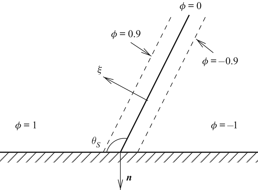
The equilibrium of the diffuse interface with mixing energy (2.2) requires
 \begin{equation} G=\lambda\left(-\frac{{\textrm{d}}^{2} \phi}{{\textrm{d}} \xi^{2}} +f_0'(\phi)\right)=0, \end{equation}
where we have considered the fact that  $\phi$ is only dependent on
 $\xi$ for the planar interface (Yue et al. Reference Yue, Feng, Liu and Shen2004). Multiplying this equation by
 ${{\textrm {d}} \phi }/{{\textrm {d}}\xi }$ gives
 \begin{equation} \frac{1}{2}\frac{{\textrm{d}}}{{\textrm{d}}\xi}\left(\frac{{\textrm{d}} \phi}{{\textrm{d}} \xi}\right)^{2} =\frac{{\textrm{d}}f_0}{{\textrm{d}} \xi}. \end{equation}
Since  $f_0=0$ and
 ${{\textrm {d}} \phi }/{{\textrm {d}} \xi }=0$ at
 $\xi =\pm \infty$, this equation can be integrated to give
 \begin{equation} \frac{{\textrm{d}} \phi}{{\textrm{d}} \xi} =\sqrt{2 f_0} = \frac{1-\phi^{2}}{\sqrt 2 \epsilon}. \end{equation}
It should be noted that the hyperbolic tangent profile  $\phi (\xi )=\tanh ({\xi }/{\sqrt 2 \epsilon })$ can be obtained by further integrating (A 3) and taking
 $\phi (\pm \infty )=\pm 1$.
When the planar interface intersects the wall with angle  $\theta _S$, we get
 \begin{equation} \lambda \boldsymbol{n} \boldsymbol{\cdot} \boldsymbol{\nabla}\phi = \lambda (\boldsymbol{n}\boldsymbol{\cdot}\boldsymbol{e}_\xi) \frac{{\textrm{d}} \phi}{{\textrm{d}}\xi}=\lambda \cos\theta_S \frac{1-\phi^{2}}{\sqrt 2 \epsilon}=\frac{3}{4}\sigma\cos\theta_S (1-\phi^{2}), \end{equation}
where  $\boldsymbol {e}_\xi = {\boldsymbol {\nabla }\phi }/{|\boldsymbol {\nabla } \phi |}$ is the unit vector in the direction of
 $\xi$ and we have used
 $\sigma =({2\sqrt 2}/{3})({\lambda }/{\epsilon })$. Meanwhile, the equilibrium at the contact line requires
 \begin{equation} L(\phi,\boldsymbol{\nabla}\phi;\theta_S)= \lambda \boldsymbol{n}\boldsymbol{\cdot} \boldsymbol{\nabla}\phi + f_w'(\phi)=0, \end{equation}
from which we can obtain the wall energy
 \begin{equation} f_w(\phi)= -\int \frac{3}{4}\sigma\cos\theta_S (1-\phi^{2}) \,{\textrm{d}}\phi = -\sigma\frac{\phi(3-\phi^{2})}{4}\cos \theta_S + c, \end{equation}
where  $c$ is an integration constant. Theoretically,
 $c$ is determined by the interfacial tensions between the fluids and the solid wall. However, the exact value of
 $c$ does not matter in practice, since we only care about the variation in free energy rather than its absolute value. We simply take
 $c=0$ in our simulations.
When a planar interface intersects the wall with a dynamic angle  $\theta _D$, similar to (A 4), we obtain
 \begin{equation} \lambda \boldsymbol{n}\boldsymbol{\cdot}\boldsymbol{\nabla}\phi = \lambda \cos\theta_D \frac{1-\phi^{2}}{\sqrt 2 \epsilon}= -f_w'(\phi;\theta_D), \end{equation}
which is used in § 3 to determine the relation between  $\theta _D$ and the static contact angles
 $\theta _A$ and
 $\theta _R$. Here the definition of
 $f_w(\phi ;\theta )$ is given in (3.1). It should be noted that other forms of wall energy that do not satisfy (A 6), e.g. those in Qian, Wang & Sheng (Reference Qian, Wang and Sheng2006b), Gao & Wang (Reference Gao and Wang2014) and Luo et al. (Reference Luo, Wang and Cai2017), may lead to distortions of
 $\phi$ contours at the contact line and cannot guarantee (A 7).
Appendix B. Constitutive relations in the phase-field model
In this section, motivated by the work of Ren & E (Reference Ren and E2011b) and the review article of Gomez & van der Zee (Reference Gomez and van der Zee2017), we derive the constitutive relations in moving contact line problems based on thermodynamic principles. The same technique was also used in de Gennes & Prost (Reference de Gennes and Prost1993) to pose constitutive laws for nematic liquid crystals. Different from the work in Ren & E (Reference Ren and E2011b), we consider a general fluid domain without requiring  $\boldsymbol {n} \boldsymbol {\cdot } \boldsymbol {u} = 0$ on the boundary.
For an incompressible two-phase system in contact with a solid wall, the total free energy can be written as
 \begin{equation} \mathcal{F}=\int_\Omega \left(f_m(\phi,\boldsymbol{\nabla}\phi) + \frac{1}{2}\rho |\boldsymbol{u}|^{2}\right) {\textrm{d}}\boldsymbol{x} + \int_{\partial \Omega_w} f_w(\phi) \,{\textrm{d}}s, \end{equation}
where  $f_m$ is the mixing energy per unit volume,
 $f_w$ is the surface energy per unit area on the wall,
 $\Omega$ is the domain occupied by the two-phase system and
 $\partial \Omega _w \subset \partial \Omega$ denotes the solid wall surface which can only perform rigid-body motion. Here we have neglected external forces such as gravity, which can be easily accounted for. The fluid domain
 $\Omega$ is advected by fluid velocity
 $\boldsymbol {u}$ and
 $\partial \Omega _w$ by wall velocity
 $\boldsymbol {u}_w$. For an impermeable wall,
 $\boldsymbol {n}\boldsymbol {\cdot } (\boldsymbol {u} -\boldsymbol {u}_w) =0$ is satisfied, where
 $\boldsymbol{n}$ is the outward pointing unit normal to the boundary. We define slip velocity
 $\boldsymbol {u}_s=\boldsymbol {u} -\boldsymbol {u}_w$, and then impermeability yields
 $\boldsymbol {u}_s\boldsymbol {\cdot } \boldsymbol {n}=0$.
Different conventions have been used for tensor operations. In this work we follow Soutas-Little (Reference Soutas-Little1999) and define the tensor operations as follows:  $(\boldsymbol{\mathsf{A}}\boldsymbol {\cdot } \boldsymbol{\mathsf{B}})_{ik}=\boldsymbol{\mathsf{A}}_{ij}\boldsymbol{\mathsf{B}}_{jk}$,
 $\boldsymbol{\mathsf{A}}:\boldsymbol{\mathsf{B}}=\boldsymbol{\mathsf{A}}_{ij}\boldsymbol{\mathsf{B}}_{ij}$,
 $(\boldsymbol {a}\boldsymbol {\cdot } \boldsymbol{\mathsf{A}})_j= a_iA_{ij}$,
 $(\boldsymbol{\mathsf{A}}\boldsymbol {\cdot } \boldsymbol {a})_i=A_{ij}a_j$,
 $(\boldsymbol {a} \otimes \boldsymbol {b})_{ij}= a_ib_j$,
 $(\boldsymbol {\nabla } \boldsymbol {a})_{ij}=({\partial }/{\partial x_i}) a_j$, and
 $(\boldsymbol {\nabla }\boldsymbol {\cdot } \boldsymbol{\mathsf{A}})_j =({\partial }/{\partial x_i})\boldsymbol{\mathsf{A}}_{ij}$. Here
 $\boldsymbol{\mathsf{A}}$ and
 $\boldsymbol{\mathsf{B}}$ are second-order tensors,
 $\boldsymbol {a}$ and
 $\boldsymbol {b}$ are vectors, and we have used the Einstein summation convention over repeated indices.
The flow needs to satisfy mass conservation
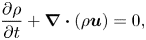 \begin{equation} \frac{\partial \rho}{\partial t} + \boldsymbol{\nabla} \boldsymbol{\cdot} (\rho \boldsymbol{u}) =0, \end{equation}
and the momentum equation
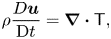 \begin{equation} \rho \frac{D\boldsymbol{u}}{\textrm{D}t} = \boldsymbol{\nabla} \boldsymbol{\cdot} \boldsymbol{\mathsf{T}}, \end{equation}
where  $\boldsymbol{\mathsf{T}}$ is the stress term to be determined later and
 ${D}/{\textrm {D}t}={\partial }/{\partial t} + \boldsymbol {u} \boldsymbol {\cdot } \boldsymbol {\nabla }$ denotes the material derivative. To conserve mass of each phase, we adopt the following equation for
 $\phi$:
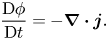 \begin{equation} \frac{\textrm{D} \phi}{\textrm{D}t}=-\boldsymbol{\nabla} \boldsymbol{\cdot} \boldsymbol{j} {. }\end{equation}
Here  $\boldsymbol {j}$ is a diffusive flux to be determined. For simplicity, we assume zero diffusive flux on the whole boundary
 $\partial \Omega$:
 $\boldsymbol{n} \boldsymbol {\cdot } \boldsymbol {j}=0$.
For the mixing energy, following the Reynolds transport theorem, we obtain
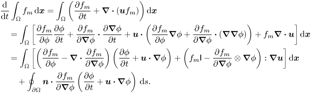 \begin{align} &\frac{{\textrm{d}}}{{\textrm{d}}t} \int_\Omega f_m \,{\textrm{d}}\boldsymbol{x} = \int_{\Omega} \left(\frac{\partial f_m}{\partial t} + \boldsymbol{\nabla}\boldsymbol{\cdot}(\boldsymbol{u} f_m) \right) {\textrm{d}}\boldsymbol{x} \nonumber\\ &\quad = \int_{\Omega} \left[ \frac{\partial f_m}{\partial \phi}\frac{\partial \phi}{\partial t} + \frac{\partial f_m}{\partial \boldsymbol{\nabla}\phi} \boldsymbol{\cdot} \frac{\partial \boldsymbol{\nabla} \phi}{\partial t} +\boldsymbol{u} \boldsymbol{\cdot} \left(\frac{\partial f_m}{\partial \phi}\boldsymbol{\nabla} \phi + \frac{\partial f_m}{\partial \boldsymbol{\nabla} \phi} \boldsymbol{\cdot} (\boldsymbol{\nabla}\boldsymbol{\nabla}\phi)\right) + f_m\boldsymbol{\nabla} \boldsymbol{\cdot} \boldsymbol{u} \right]{\textrm{d}}\boldsymbol{x} \nonumber\\ &\quad = \int_{\Omega}\left[ \left(\frac{\partial f_m}{\partial \phi}-\boldsymbol{\nabla} \boldsymbol{\cdot} \frac{\partial f_m}{\partial \boldsymbol{\nabla} \phi}\right) \left(\frac{\partial \phi}{\partial t} +\boldsymbol{u} \boldsymbol{\cdot} \boldsymbol{\nabla} \phi\right) + \left(f_m \boldsymbol{\mathsf{I}} - \frac{\partial f_m}{\partial \boldsymbol{\nabla} \phi} \otimes \boldsymbol{\nabla} \phi \right) :\boldsymbol{\nabla} \boldsymbol{u}\right]{\textrm{d}}\boldsymbol{x}\nonumber\\ &\qquad+\oint_{\partial \Omega} \boldsymbol{n} \boldsymbol{\cdot} \frac{\partial f_m}{\partial \boldsymbol{\nabla} \phi} \left(\frac{\partial \phi}{\partial t} +\boldsymbol{u} \boldsymbol{\cdot} \boldsymbol{\nabla} \phi\right) \,{\textrm{d}}s. \end{align}
Here we have recovered the chemical potential
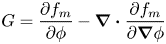 \begin{equation} G=\frac{\partial f_m}{\partial \phi}-\boldsymbol{\nabla} \boldsymbol{\cdot} \frac{\partial f_m}{\partial \boldsymbol{\nabla} \phi} \end{equation}
and the stress term due to surface tension
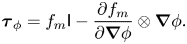 \begin{equation} \boldsymbol{\tau}_\phi =f_m\boldsymbol{\mathsf{I}} - \frac{\partial f_m}{\partial \boldsymbol{\nabla} \phi} \otimes \boldsymbol{\nabla} \phi. \end{equation}
The surface tension term (B 7) can also be obtained by the virtual work principle without imposing the incompressibility condition. Considering the conserved phase dynamics (B 4), (B 5) can be further written as
 \begin{equation} \frac{{\textrm{d}}}{{\textrm{d}}t}\int_{\Omega}f_m \,{\textrm{d}}\boldsymbol{x} = \int_{\Omega}\left(\boldsymbol{\nabla} G \boldsymbol{\cdot} \boldsymbol{j} +\boldsymbol{\tau}_\phi : \boldsymbol{\nabla} \boldsymbol{u}\right) {\textrm{d}}\boldsymbol{x} + \oint_{\partial \Omega}\left(\boldsymbol{n} \boldsymbol{\cdot} \frac{\partial f_m}{\partial \boldsymbol{\nabla} \phi} \right)\frac{\textrm{D} \phi}{\textrm{D}t}\,{\textrm{d}}s, \end{equation}
where we have used the condition  $\boldsymbol {n} \boldsymbol {\cdot } \boldsymbol {j}=0$ on
 $\partial \Omega$.
For the kinetic energy, we get
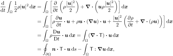 \begin{align} \frac{{\textrm{d}}}{{\textrm{d}}t}\int_\Omega \frac{1}{2}\rho |\boldsymbol{u}|^{2} \,{\textrm{d}}\boldsymbol{x} & = \int_{\Omega}\left[ \frac{\partial}{\partial t} \left(\rho\frac{|\boldsymbol{u}|^{2}}{2}\right) + \boldsymbol{\nabla}\boldsymbol{\cdot}\left(\boldsymbol{u} \rho \frac{|\boldsymbol{u}|^{2}}{2}\right) \right]{\textrm{d}}\boldsymbol{x} \nonumber\\ &= \int_{\Omega}\left[ \rho \frac{\partial \boldsymbol{u}}{\partial t} \boldsymbol{\cdot} \boldsymbol{u}+ \rho \boldsymbol{u} \boldsymbol{\cdot} (\boldsymbol{\nabla} \boldsymbol{u}) \boldsymbol{\cdot} \boldsymbol{u} + \frac{|\boldsymbol{u}|^{2}}{2}\left(\frac{\partial \rho}{\partial t} +\boldsymbol{\nabla} \boldsymbol{\cdot} (\rho\boldsymbol{u}) \right) \right]{\textrm{d}}\boldsymbol{x} \nonumber\\ &= \int_{\Omega} \rho \frac{\textrm{D}\boldsymbol{u}}{\textrm{D}t}\boldsymbol{\cdot} \boldsymbol{u} \,{\textrm{d}}\boldsymbol{x}= \int_{\Omega} (\boldsymbol{\nabla}\boldsymbol{\cdot} \boldsymbol{\mathsf{T}})\boldsymbol{\cdot} \boldsymbol{u} \,{\textrm{d}}\boldsymbol{x}\nonumber\\ & =\oint_{\partial\Omega} \boldsymbol{n}\boldsymbol{\cdot}\boldsymbol{\mathsf{T}}\boldsymbol{\cdot} \boldsymbol{u} \,{\textrm{d}}s -\int_{ \Omega} \boldsymbol{\mathsf{T}}: \boldsymbol{\nabla} \boldsymbol{u} \,{\textrm{d}}\boldsymbol{x}, \end{align}
where we have used (B 2) in the third equality and (B 3) in the fourth equality.
Different from the mixing and kinetic energies, the wall energy is associated with the solid wall and is thus advected by  $\boldsymbol {u}_w$ instead of
 $\boldsymbol {u}$. Since the wall surface is rigid (thus, the surface divergence of
 $\boldsymbol {u}_w$ vanishes), we have
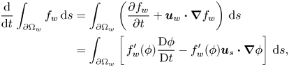 \begin{align} \frac{{\textrm{d}}}{{\textrm{d}}t}\int_{\partial \Omega_w}f_w \,{\textrm{d}}s & = \int_{\partial\Omega_w} \left(\frac{\partial f_w}{\partial t} +\boldsymbol{u}_w \boldsymbol{\cdot} \boldsymbol{\nabla} f_w\right)\,{\textrm{d}}s \nonumber\\ &=\int_{\partial\Omega_w} \left[\,f_w'(\phi) \frac{\textrm{D} \phi}{\textrm{D}t} -f_w'(\phi)\boldsymbol{u}_s \boldsymbol{\cdot} \boldsymbol{\nabla}\phi\right] \,{\textrm{d}}s, \end{align}
where we have used the relation  $\boldsymbol {u}_s=\boldsymbol {u}- \boldsymbol {u}_w$.
Summing up (B 8), (B 9) and (B 10), we arrive at the energy equation
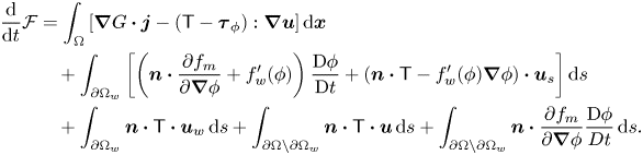 \begin{align} \frac{{\textrm{d}}}{{\textrm{d}}t}{\mathcal{F}} & = \int_{\Omega} \left[\boldsymbol{\nabla} G \boldsymbol{\cdot} \boldsymbol{j} - (\boldsymbol{\mathsf{T}} -\boldsymbol{\tau}_\phi):\boldsymbol{\nabla}\boldsymbol{u}\right] {\textrm{d}}\boldsymbol{x} \nonumber\\ &\quad + \int_{\partial \Omega_w} \left[\left(\boldsymbol{n}\boldsymbol{\cdot} \frac{\partial f_m}{\partial \boldsymbol{\nabla} \phi} + f_w'(\phi)\right)\frac{\textrm{D} \phi}{\textrm{D}t} + (\boldsymbol{n}\boldsymbol{\cdot} \boldsymbol{\mathsf{T}} -f_w'(\phi)\boldsymbol{\nabla}\phi)\boldsymbol{\cdot} \boldsymbol{u}_s \right]{\textrm{d}}s \nonumber\\ &\quad + \int_{\partial\Omega_w} \boldsymbol{n} \boldsymbol{\cdot} {\boldsymbol{\mathsf{T}}}\boldsymbol{\cdot} \boldsymbol{u}_w \,{\textrm{d}}s + \int_{\partial\Omega\backslash \partial\Omega_w} \boldsymbol{n} \boldsymbol{\cdot} {\boldsymbol{\mathsf{T}}} \boldsymbol{\cdot} \boldsymbol{u} \,{\textrm{d}}s + \int_{\partial\Omega\backslash \partial\Omega_w} \boldsymbol{n} \boldsymbol{\cdot} \frac{\partial f_m}{\partial \boldsymbol{\nabla} \phi} \frac{\textrm{D} \phi}{D t} \,{\textrm{d}}s. \end{align}
Here we have recovered the surface potential on the wall boundary  $\partial \Omega _w$:
 \begin{equation} L(\phi,\boldsymbol{\nabla}\phi)=\boldsymbol{n}\boldsymbol{\cdot} \frac{\partial f_m}{\partial \boldsymbol{\nabla} \phi} + f_w'(\phi). \end{equation}
The first two terms on the right-hand side of (B 11) denote the dissipation rate in the system, which corresponds to entropy production due to irreversible processes. The third and fourth terms account for the work done by the moving wall and other boundaries. The last term vanishes if we impose  $\boldsymbol {n} \boldsymbol {\cdot } ({\partial f_m}/{\partial \boldsymbol {\nabla } \phi })=0$ on
 $\partial \Omega \backslash \partial \Omega _w$, i.e. the interface is perpendicular to the boundary. This corresponds to a neutral wetting condition, which is automatically satisfied if we use homogeneous natural boundary conditions for the Cahn–Hilliard equation on boundaries other than the wall.
The dissipation terms in (B 11) have been written in the form of products of the ‘generalized flux’ and the corresponding ‘generalized force’. According to the second law of thermodynamics, the irreversible processes must be entropy-productive, i.e. the associated energy dissipation rate must be non-negative. If we assume linear response then energy dissipation is satisfied if we take
 \begin{gather} \boldsymbol{j} = -M\boldsymbol{\nabla} G \quad\mbox{in } \Omega, \end{gather}
 \begin{gather}\boldsymbol{\mathsf{T}}= -\mu (\boldsymbol{\nabla} \boldsymbol{u} +(\boldsymbol{\nabla}\boldsymbol{u})^{T}) +\boldsymbol{\tau}_\phi \quad \mbox{in } \Omega, \end{gather}
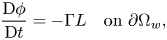 \begin{gather}\frac{\textrm{D} \phi}{\textrm{D}t}=-\Gamma L \quad \mbox{on }\partial \Omega_w, \end{gather}
 \begin{gather}-\beta \boldsymbol{u}_s= (\boldsymbol{n}\boldsymbol{\cdot} \boldsymbol{\mathsf{T}} -f_w'(\phi)\boldsymbol{\nabla}\phi)\boldsymbol{\cdot} (\boldsymbol{\mathsf{I}}-\boldsymbol{n} \otimes \boldsymbol{n}) \quad \mbox{on }\partial \Omega_w, \end{gather}
with some positive parameters  $M$,
 $\mu$,
 $\Gamma$ and
 $\beta$. It should be noted that there might be other energy-dissipative constitutive relations than (B 13)–(B 16) and additional conditions are required to determine the physically correct constitutive relations. In (B 14) we have assumed that
 ${\boldsymbol{\mathsf{T}}}-\boldsymbol {\tau }_\phi$ is a symmetric tensor, which is usually the case for physically relevant systems. In (B 16) we have used
 $\boldsymbol {u}_s= (\boldsymbol{\mathsf{I}} -\boldsymbol {n}\otimes \boldsymbol {n})\boldsymbol {\cdot } \boldsymbol {u}_s$ which is a direct result of the impermeability condition
 $\boldsymbol {n}\boldsymbol {\cdot }\boldsymbol {u}_s=0$.
Plugging (B 13) into (B 4), we arrive at the Cahn–Hilliard equation
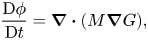 \begin{equation} \frac{\textrm{D} \phi}{\textrm{D}t}= \boldsymbol{\nabla}\boldsymbol{\cdot} (M\boldsymbol{\nabla} G), \end{equation}
where  $M$ is called the mobility parameter.
For incompressible flows,  $\boldsymbol{\mathsf{I}} : \boldsymbol {\nabla } \boldsymbol {u} =\boldsymbol {\nabla }\boldsymbol {\cdot } \boldsymbol {u} = 0$; thus, an isotropic term
 $-p \boldsymbol{\mathsf{I}}$ can be added to
 ${\boldsymbol{\mathsf{T}}}$ without affecting dissipation. This parameter
 $p$, interpreted as pressure, serves as a Lagrange multiplier to enforce incompressibility. The momentum equation (B 3) thus reads as
 \begin{equation} \rho\frac{D\boldsymbol{u}}{\textrm{D}t}=\boldsymbol{\nabla} \boldsymbol{\cdot} \left[-p\boldsymbol{\mathsf{I}} +\mu \left(\boldsymbol{\nabla}\boldsymbol{u} +(\boldsymbol{\nabla}\boldsymbol{u})^{T} \right)+\boldsymbol{\tau}_\phi\right]. \end{equation}
It should be noted that different forms of  $\boldsymbol {\tau }_\phi$ have been used in the literature. For example, the isotropic term
 $f_m \boldsymbol{\mathsf{I}}$ can be absorbed into
 $p\boldsymbol{\mathsf{I}}$ such that one can effectively use
 $\tilde{\boldsymbol {\tau }}_\phi =- {\partial f_m}/{\partial \boldsymbol {\nabla } \phi } \otimes \boldsymbol {\nabla } \phi$ to replace
 $\boldsymbol {\tau }_\phi$ (Yue et al. Reference Yue, Feng, Liu and Shen2004). The forcing term due to
 $\boldsymbol {\tau }_\phi$ can also be written as
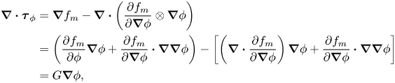 \begin{align} \boldsymbol{\nabla}\boldsymbol{\cdot} \boldsymbol{\tau}_\phi & =\boldsymbol{\nabla} f_m - \boldsymbol{\nabla}\boldsymbol{\cdot} \left( \frac{\partial f_m}{\partial \boldsymbol{\nabla} \phi}\otimes \boldsymbol{\nabla}\phi \right) \nonumber\\ &= \left(\frac{\partial f_m}{\partial \phi}\boldsymbol{\nabla}\phi + \frac{\partial f_m}{\partial \boldsymbol{\nabla}\phi}\boldsymbol{\cdot} \boldsymbol{\nabla}\boldsymbol{\nabla}\phi\right)-\left[ \left(\boldsymbol{\nabla}\boldsymbol{\cdot} \frac{\partial f_m}{\partial \boldsymbol{\nabla} \phi}\right)\boldsymbol{\nabla} \phi + \frac{\partial f_m}{\partial \boldsymbol{\nabla} \phi}\boldsymbol{\cdot} \boldsymbol{\nabla}\boldsymbol{\nabla}\phi\right] \nonumber\\ &=G\boldsymbol{\nabla}\phi, \end{align}
which is adopted in this work. Alternatively, a body force of the form  $-\phi \boldsymbol {\nabla } G=G\boldsymbol {\nabla }\phi -\boldsymbol {\nabla }(G\phi )$ was also found in the literature (Jacqmin Reference Jacqmin2000).
On the solid wall, the wall energy relaxation is governed by (B 15). Equation (B 16) is exactly the generalized Navier boundary condition (Qian, Wang & Sheng Reference Qian, Wang and Sheng2006a; Qian et al. Reference Qian, Wang and Sheng2006b), which was originally derived based on Onsager's principle of minimum energy dissipation. It should be noted that the no-slip condition  $\boldsymbol {u}_s=0$, adopted by us and many others (Jacqmin Reference Jacqmin2000; Khatavkar et al. Reference Khatavkar, Anderson and Meijer2007b; Carlson, Do-Quang & Amberg Reference Carlson, Do-Quang and Amberg2009), provides a simpler formulation which also satisfies energy dissipation.
Appendix C. Compressibility and Mass diffusion
For incompressible flows, we usually impose  $\boldsymbol {\nabla }\boldsymbol {\cdot } \boldsymbol {u}=0$. The mixture density
 $\rho$ is governed by mass conservation (B 2). Meanwhile, given the densities of the pure phases, the mixture density can also be expressed as a function of the phase-field variable
 $\phi$, and is therefore governed by the phase-field equation (B 17) unless
 $\rho '(\phi )=0$. Thus, the system in appendix B. may be over-determined if the two phases have different densities. To remedy this, the governing equations need to be modified and there are primarily two ways to derive physically consistent models.
The first method, proposed by Lowengrub & Truskinovsky (Reference Lowengrub and Truskinovsky1998), is to consider the system as quasi-incompressible. In this treatment,  $\phi$ is associated with mass fraction and the mixture velocity
 $\boldsymbol {u}$ is interpreted as the mass-averaged velocity. Then, from mass conservation (B 2), we can obtain
 \begin{equation} \boldsymbol{\nabla}\boldsymbol{\cdot} \boldsymbol{u} = -\frac{1}{\rho}\frac{\textrm{D}\rho}{\textrm{D}t} = -\frac{\rho'(\phi)}{\rho}\frac{\textrm{D} \phi}{\textrm{D}t}, \end{equation}
where  ${\textrm {D} \phi }/{\textrm {D}t}$ is determined by the Cahn–Hilliard equation. This equation replaces the original
 $\boldsymbol {\nabla }\boldsymbol {\cdot } \boldsymbol {u}=0$. Moreover, due to compressibility, the mixing energy
 $f_m$ has to be interpreted as a free energy per unit mass (and, thus, the total mixing energy is
 $\int _\Omega \rho f_m\,{\textrm {d}}\boldsymbol {x})$, which will cause substantial changes to the governing equations. Applications of this method can be found in Guo, Lin & Lowengrub (Reference Guo, Lin and Lowengrub2014) and Guo & Lin (Reference Guo and Lin2015).
The other method, first proposed by Ding, Spelt & Shu (Reference Ding, Spelt and Shu2007) and later improved by Abels et al. (Reference Abels, Garcke and Grün2012), associates  $\phi$ with volume fraction and interprets
 $\boldsymbol {u}$ as the volume-averaged velocity. It can be easily shown that
 $\boldsymbol {\nabla }\boldsymbol {\cdot } \boldsymbol {u}=0$ is still satisfied. However, this volume-averaged velocity modifies the mass conservation equation (B 2) to
 \begin{equation} \frac{\partial \rho}{\partial t} + \boldsymbol{\nabla}\boldsymbol{\cdot}(\rho \boldsymbol{u}) + \boldsymbol{\nabla}\boldsymbol{\cdot} \boldsymbol{J}=0, \end{equation}
where  $\boldsymbol{J}$ is the diffusive mass flux. It is obvious that
 \begin{equation} \boldsymbol{\nabla}\boldsymbol{\cdot} J=-\frac{\textrm{D}\rho}{\textrm{D}t} = -\rho'(\phi) \frac{\textrm{D} \phi}{\textrm{D}t}. \end{equation}
Comparing this equation with (B 4) and considering the fact that  $\rho '(\phi )$ is usually a constant (see (2.16) for an example), we arrive at the identity
 \begin{equation} \boldsymbol{J}=\rho'(\phi) \boldsymbol{j}. \end{equation}
Considering (C 2) and the Galilean invariance requirement, the momentum equation (B 3) is updated to
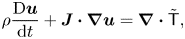 \begin{equation} \rho \frac{\textrm{D}\boldsymbol{u}}{{\textrm{d}}t} + \boldsymbol{J} \boldsymbol{\cdot} \boldsymbol{\nabla} \boldsymbol{u} = \boldsymbol{\nabla} \boldsymbol{\cdot} \tilde{\boldsymbol{\mathsf{T}}}, \end{equation}
where  $\tilde{\boldsymbol{\mathsf{T}}} = \boldsymbol{\mathsf{T}} + \boldsymbol{J} \otimes \boldsymbol {u}$ is an objective tensor that replaces the original
 $\boldsymbol{\mathsf{T}}$ in (B 3). The interested reader may refer to Abels et al. (Reference Abels, Garcke and Grün2012) for detailed derivations and Dong (Reference Dong2014, Reference Dong2015) for extensions to
 $N$-phase systems with
 $N\ge 2$. It should be noted that the original formulation in Ding et al. (Reference Ding, Spelt and Shu2007) is not Galilean invariant.
The method by Abels et al. allows us to use the existing numerical algorithms for incompressible flows with very little modification, and is thus more frequently seen in the recent literature (e.g. Shen & Yang Reference Shen and Yang2015; Yu & Yang Reference Yu and Yang2017). In the following we only focus on this method.
With the modified mass conservation (C 2) and momentum equation (C 5), the time derivative of kinetic energy is updated to
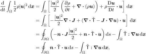 \begin{align} \frac{{\textrm{d}}}{{\textrm{d}}t}\int_\Omega \frac{1}{2}\rho|\boldsymbol{u}|^{2} \,{\textrm{d}}\boldsymbol{x} & = \int_\Omega \left[\frac{|\boldsymbol{u}|^{2}}{2} \left(\frac{\partial \rho}{\partial t} + \boldsymbol{\nabla} \boldsymbol{\cdot} (\rho\boldsymbol{u}) \right) + \rho \frac{\textrm{D} \boldsymbol{u}}{\textrm{D}t}\boldsymbol{\cdot} \boldsymbol{u} \right]\,{\textrm{d}}\boldsymbol{x} \nonumber\\ & = \int_{\Omega} \left[-\frac{|\boldsymbol{u}|^{2}}{2}\boldsymbol{\nabla}\boldsymbol{\cdot} \boldsymbol{J} + (\boldsymbol{\nabla}\boldsymbol{\cdot} \tilde{\boldsymbol{\mathsf{T}}} - \boldsymbol{J}\boldsymbol{\cdot} \boldsymbol{\nabla} \boldsymbol{u}) \boldsymbol{\cdot} \boldsymbol{u}\right]\,{\textrm{d}}\boldsymbol{x} \nonumber\\ & =\oint_{\partial \Omega} \left(-\boldsymbol{n} \boldsymbol{\cdot} \boldsymbol{J} \frac{|\boldsymbol{u}|^{2}}{2} +\boldsymbol{n}\boldsymbol{\cdot} \tilde{\boldsymbol{\mathsf{T}}} \boldsymbol{\cdot} \boldsymbol{u} \right){\textrm{d}}s - \int_{\Omega} \tilde{\boldsymbol{\mathsf{T}}}:\boldsymbol{\nabla}\boldsymbol{u}\,{\textrm{d}}\boldsymbol{x} \nonumber\\ & =\oint_{\partial \Omega} \boldsymbol{n}\boldsymbol{\cdot} \tilde{\boldsymbol{\mathsf{T}}} \boldsymbol{\cdot} \boldsymbol{u} \,{\textrm{d}}s - \int_{\Omega} \tilde{\boldsymbol{\mathsf{T}}}:\boldsymbol{\nabla}\boldsymbol{u}\,{\textrm{d}}\boldsymbol{x}{, } \end{align}
where we have used the zero-diffusive-flux condition  $\boldsymbol {n}\boldsymbol {\cdot } \boldsymbol{J}=\rho '(\phi )\boldsymbol {n} \boldsymbol {\cdot } \boldsymbol {j}=0$ on the boundary. This equation is identical to (B 9) except for a different interpretation of the stress tensor. Consequently, all the equations remain the same as those in appendix B, except for the modified mass conservation and momentum equations.
In our computations on oscillating drops (see figure 17d), however, we did not find any noticeable difference between the results from (B 3) and (C 5). Thus, in practice, the effect of compressibility is only limited to the diffuse interface and has negligible effect on the macroscopic flow.