








1. Introduction
We consider the three-dimensional incompressible non-stationary Navier–Stokes equations

Here $u$ describes the velocity of the flow and the scalar function $\Pi$
 represents the pressure of the fluid. The initial data $u_{0}(x)$
 satisfies the divergence-free condition.
The full regularity of solutions of the three-dimensional Navier–Stokes equations is not known, the partial regularity theory of suitable weak solutions of this system starting from Scheffer's work [Reference Scheffer23–Reference Scheffer25] is well-known. The famous Caffarelli–Kohn–Nirenberg theorem in [Reference Caffarelli, Kohn and Nirenberg4] is that the one-dimensional parabolic Hausdorff measure of the potential space–time singular points set $\mathcal {S}$ of suitable weak solutions to the 3D Navier–Stokes equations is zero. The critical tool is the following so-called $\epsilon$
 -regularity criterion: there is an absolute constant $\epsilon$
 such that if

then $u$ is bounded in a neighbourhood of $(0,0)$
 , where $Q(\varrho ):=B(\varrho )\times (-\varrho ^{2},0)$
 and $B(\varrho )$
 denotes the ball of centre $0$
 and radius $\varrho$
 . To this end, Caffarelli–Kohn–Nirenberg [Reference Caffarelli, Kohn and Nirenberg4] established an $\epsilon$
 -regularity criterion at one scale

An alternative approach of Caffarelli–Kohn–Nirenberg theorem based on blow-up argument was due to Lin, Ladyzhenskaya and Seregin [Reference Ladyzenskaja and Seregin17, Reference Lin18], where the corresponding $\epsilon$ -regularity criterion at one scale reads

In what follows, a point $z=(x,t)$ in (1.1) is said to be regular if $u$
 belongs to $L^{\infty }$
 at a neighbourhood of $z$
 . Otherwise, it is called singular. Estimates of the size of potential singular points set in the 3D Navier–Stokes equations can be found in [Reference Barker and Wang1, Reference Gustafson, Kang and Tsai9, Reference Kukavica14, Reference Kukavica and Pei15, Reference Robinson and Sadowski20–Reference Robinson and Sadowski22, Reference Wang and Zhang30, Reference Wang and Wu31].
On the other hand, the integral (Serrin) type conditions based on the velocity, the gradient of the velocity or the pressure lead to the full regularity of Leray–Hopf weak solutions of the 3D Navier–Stokes equations. Precisely, a weak solution $u$ is smooth on $(0,T]$
 if it satisfies one of the following three conditions
(1) Serrin [Reference Serrin27], Struwe [Reference Struwe26], Escauriaza, Seregin and Šverák [Reference Escauriaza, Seregin and Šverák7]
(1.5)\begin{equation} u\in L^{p} (0,T;L^{q}( \mathbb{R}^{3}))\ \text{with}\ 2/p+3/q=1, \quad q\geq3. \end{equation}
(2) Beirao da Veiga [Reference Beirao da Veiga2]
(1.6)\begin{equation} \nabla u\in L^{p} (0,T;L^{q}( \mathbb{R}^{3}))\ \text{with}\ 2/p+3/q=2,\quad q>3/2. \end{equation}
(3) Berselli and Galdi [Reference Berselli and Galdi3], Zhou [Reference Zhou36, Reference Zhou37]
(1.7)\begin{equation} \Pi \in L^{p} (0,T;L^{q}( \mathbb{R}^{3}))\ \text{with}\ 2/p+3/q=2 , \quad q>3/2. \end{equation}


The aforementioned integral (Serrin) type conditions can be seen as the critical regularity, which is scale invariant under the natural scaling of the Navier–Stokes equations (1.1). The full regularity means that the set of $\mathcal {S}$ is empty. The natural (supercritical) regularity $u \in L^{q}(0,\,T;\,L^{p}(\mathbb {R}^{3}))$
 with $\frac 2q+\frac 3p=\frac 32$
 in suitable weak solutions means that

which can be found in [Reference Caffarelli, Kohn and Nirenberg4, Reference Robinson and Sadowski20] and $\dim _{H}(S)$ and $\dim _{B}(S)$
 denote the Hausdorff dimension and box dimension of a set $S$
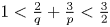
 , respectively. A natural question is whether the suitable weak solutions satisfying supercritical regularity $u \in L^{q}(0,\, T;\,L^{p}(\mathbb {R}^{3}))$
 with $1<\frac 2q+\frac 3p<\frac 32$
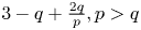
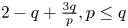
 lower the fractal dimension in (1.8). In this direction, Gustafson, Kang and Tsai [Reference Gustafson, Kang and Tsai9] proved that the Hausdorff dimension of the potential singular points set $\mathcal {S}$
 of a Leray–Hopf weak solution belonging to $u\in L^{q}(0,T;L^{p}(\mathbb {R}^{3}))$
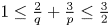
 for $1\leq \frac {2}{q}+\frac {3}{p}$
 with $\frac 2p+\frac 2q<1$
 and $\frac 3p+\frac 1q<1$
 is at most $3-q+\frac {2q}{p}, p>q$
 or $2-q+\frac {3q}{p}, p\leq q$
 . Robinson and Sadowski [Reference Robinson and Sadowski22] showed that the upper box dimension of potential singular points set $\mathcal {S}$
 of a suitable weak solution belonging to $u\in L^{q}(0,T;L^{p}(\mathbb {R}^{3}))$
 for $1\leq \frac {2}{q}+\frac { 3}{p} \leq \frac 32$
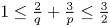 with $3< p,q<\infty$
 is no greater than

In addition, the Hausdorff dimension of potential singular points set $\mathcal {S}$ of a suitable weak solution belonging to $\nabla u\in L^{q}(0,T;L^{p}(\mathbb {R}^{3}))$
 for $2\leq \frac {2}{q}+\frac {3}{p} \leq \frac 52$
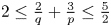 with $2< p\leq q<\infty$
 is less than or equal to

In [Reference Robinson and Sadowski22, Conclusion, Page 9], Robinson and Sadowski mentioned some natural questions from their results:
(1) It would be interesting to relax the assumption $q> 3$
in (1.9) and obtain the same bound for any $q \geq 2$;(2) Similarly in (1.10) one would like to relax the condition $q\geq p$
.(3) In order to obtain (1.9) in a bounded domain we would require the analogue of Lemma 2 (estimates for the pressure when $u\in L^{q}(0,T;L^{p}(\Omega ))$
.(4) An order of magnitude harder is to determine whether any of these partial regularity results can be proved for general weak solutions, and not only suitable weak solutions.



In this paper, our first result is the following theorem.
Theorem 1.1 Let $u$ be a suitable weak solution belonging to $u\in L^{q}(0,T;L^{p}(\mathbb {R}^{3}))$
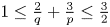
 for $1\leq \frac {2}{q}+\frac { 3}{p}\leq \frac 32$
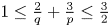 with $2\leq q<\infty$
 and $2< p<\infty$
 . Then, the upper box dimension of its potential singular points set $\mathcal {S}$
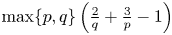
 is at most $\max \{p,q\}\left (\frac {2}{q}+\frac {3}{p}-1\right )$
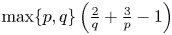 .
Remark 1.2 Theorem 1.1 answers Robinson and Sadowski's first question (1).
As observed in [Reference Gustafson, Kang and Tsai9], the weak solutions in spaces $L^{q}(0,T;L^{p}(\mathbb {R}^{3}))$ with $\frac 2p+\frac 2q<1$
 and $\frac 3p+\frac 1q<1$
 are suitable weak solutions. Therefore, towards the Robinson and Sadowski's fourth question (4), we have
Corollary 1.3 Let $u$ be a Leray–Hopf weak solution belonging to $u\in L^{q}(0,T;L^{p}(\mathbb {R}^{3}))$
 for $1\leq \frac {2}{q}+\frac { 3}{p}\leq \frac 32$
 with $\frac 2p+\frac 2q<1$
 and $\frac 3p+\frac 1q<1$
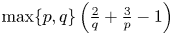
 . Then, the upper box dimension of its potential singular points set $\mathcal {S}$
 is at most $\max \{p,q\}\left (\frac {2}{q}+\frac {3}{p}-1\right )$
 .
With a slight modification of the proof of theorem 1.1 and using the $\epsilon$ -regularity criterion at one scale without pressure in [Reference Wang, Wu and Zhou33], we can obtain a parallel result of (1.9) in a bounded domain, which is corresponding to Robinson and Sadowski's third issue.
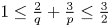
Theorem 1.4 Let $u$ be a suitable weak solution belonging to $u\in L^{q}(0,T;L^{p}(\Omega ))$
 for $1\leq \frac {2}{q}+\frac { 3}{p}\leq \frac 32$
 with $\frac 52< q,p<\infty$
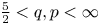 . Then, the upper box dimension of its interior potential singular points set $\mathcal {S}$
 is at most $\max \{p,q\}\left (\frac {2}{q}+\frac {3}{p}-1\right )$
 .
Robinson–Sadowski results on $\mathbb {R}^{3}$ .

Theorem 1.1 on $\mathbb {R}^{3}$ .

Corollary 1.3 weak solutions.

Theorem 1.4 on bounded domain.

Roughly, the following figures (Figures 1–4) summarize the known upper box dimension of its potential singular points set $\mathcal {S}$ of suitable weak solutions under supercritical regularity in the Navier–Stokes equations.
Next, we study the Robinson and Sadowski's second issue involving the gradient of the velocity with additional regularity. It seems that this problem is more complicated. Very recently, in the other direction, Barker and Wang [Reference Barker and Wang1] estimate the Hausdorff dimension of the singular set for the Navier–Stokes equations with supercritical assumptions on the pressure. There are two new ingredients in their proof. The first one is the higher integrability of the solutions with certain supercritical assumptions on pressure in the Navier–Stokes equations. The second one is the $\epsilon$ -regularity criterion in terms of quantity $|\nabla u|^{2}|u|^{q-2}$
 with $2< q<3$
 , which usually arises in the $L^{p}$
 type energy estimates of the Navier–Stokes equations. In the spirit of [Reference Barker and Wang1], we consider the $\epsilon$
 -regularity criterion via quantity $\Lambda ^{s+1}u$
 with $s>0$
 , which usually appears in the $\dot {H}^{s+1}$
 type energy estimates of the Navier–Stokes equations. One naturally invokes the Caffarelli–Silvestre extension used in [Reference Colombo, De Lellis and Massaccesi6, Reference Ren, Wang and Wu19, Reference Tang and Yu29] to overcome non-local derivatives. However, since $s>0$
 , one requires higher-order Caffarelli–Silvestre (Yang) extensions [Reference Yang35]. To this end, we observe that the following identity due to [Reference Colombo, De Lellis and Massaccesi6], for $\alpha =s+1>1$
 ,

that is,

which helps us to reduce the proof of theorem 1.5 to show theorem 1.6 just by Caffarelli–Silvestre extension rather than higher-order (Yang) extension. Theorem 1.5 can be viewed as the interpolation between the Caffarelli–Kohn–Nirenberg theorem and Kozono-Taniuchi regular class $L^{2}(0,T; BMO)$ , which is of independent interest.
Theorem 1.5 Let $u$ be a suitable weak solution belonging to $u\in L^{2}(0,T;\dot {H}^{s+1}(\mathbb {R}^{3}))$
 for $0\leq s\leq \frac 12$
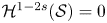
 . Then, $\mathcal {H}^{ 1-2 s}(\mathcal {S})=0$
 .
Proposition 1.6 Suppose that $u$ is a suitable weak solution to (1.1). Then there exists an absolute positive constant $\epsilon _{01}$
 such that $(0,0)$
 is a regular point if

First part of corollary 1.7.

Second part of corollary 1.7.

Known Hausdorff dimension of the gradient of the velocity.

As an application of theorem 1.5 and the energy estimate of the Navier–Stokes equations, we can partially answer the Robinson and Sadowski's second question.
Corollary 1.7 Let $u$ be a suitable weak solution belonging to $\nabla u\in L^{q}(0,T;L^{p}(\mathbb {R}^{3}))$
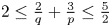
 for $2\leq \frac {2}{q}+\frac { 3}{p}\leq \frac 52$
 .
(1) If $\frac 52-\frac 3p-\frac {5}{2q}\geq 0,2< p<\frac {54+12\sqrt {14}}{25}, 1< q\leq 2$
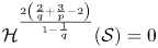
, then $\mathcal {H}^{ \frac {2\left (\frac {2}{q}+\frac {3}{p}-2\right )}{1-\frac 1q}}(\mathcal {S})=0$.(2) If $2-\frac 3p-\frac 1q\geq 0,\frac 32< p<\frac {12}{7},q\geq 4$
, then $\mathcal {H}^{q\left (\frac {2}{q}+\frac {3}{p}-2\right )}(\mathcal {S})=0$.



Currently, the Hausdorff dimension of suitable weak solutions with the gradient of the velocity under supercritical regularity are summarized in the following figures (Figures 5–7).
The remainder of this paper is organized as follows. In §2, we begin with the notations and the definition of fractal dimension including the Box dimension and Hausdorff dimension. Then we recall the Caffarelli and Silvestre's generalized extension for the fractional Laplacian operator and $\epsilon$ -regularity criterion at one scale. Section 3 is devoted to the proof of theorem 1.1 concerning Box dimension. Partial regularity results involving Hausdorff dimension is proved in §4.
2. Preliminaries
First, we introduce some notations used in this paper. Throughout this paper, we denote

For $p\in [1,\,\infty ]$ , the notation $L^{p}(0,\,T;X)$
 stands for the set of measurable functions on the interval $(0,\,T)$
 with values in $X$
 and $\|f(\cdot,t)\|_{X}$
 belonging to $L^{p}(0,\,T)$
 . For simplicity, we write $\|f\| _{L^{p,q}(Q(\mu ))}:=\|f\| _{L^{p}(-\mu ^{2},0;L^{q}(B(\mu )))}$
 and $\|f\| _{L^{p}(Q(\mu ))}:=\|f\| _{L^{p}L^{p}(Q(\mu ))}$
 . We shall denote by $\langle f,\,g\rangle$
 the $L^{2}$
 inner product of $f$
 and $g$
 . The classical Sobolev norm $\|\cdot \|_{H^{s}}$
 is defined as $\|f\|^{2} _{{H}^{s}}= \int _{\mathbb {R}^{n}} (1+|\xi |)^{2s}|\hat {f}(\xi )|^{2}\,{\rm d}\xi$
 , $s\in \mathbb {R}$
 . We denote by $\dot {H}^{s}$
 homogenous Sobolev spaces with the norm $\|f\|^{2} _{\dot {H}^{s}}= \int _{\mathbb {R}^{n}} |\xi |^{2s}|\hat {f}(\xi )|^{2}\,{\rm d}\xi$
 . Denote the average of $f$
 on the ball $B(\mu )$
 by $\overline {f}_{\mu }$
 . $\Gamma$
 denotes the standard normalized fundamental solution of Laplace equation in $\mathbb {R}^{3}$
 . We denote by $\text {Div}$
 the divergence operator in $\mathbb {R}^{n+1}$
 and $\nabla ^{\ast }$
 the gradient operator in $\mathbb {R}^{n+1}$
 . $|S|$
 represents the Lebesgue measure of the set $S$
 . We will use the summation convention on repeated indices. $C$
 is an absolute constant which may be different from line to line unless otherwise stated in this paper.
Definition 2.1 The (upper) box-counting dimension of a set $X$ is usually defined as

where $N(X,\,\epsilon )$ is the minimum number of balls of radius $\epsilon$
 required to cover $X$
 .
Let $\beta >0$ , $\delta >0$
 and $\Omega \times I$
 can be covered by the union of series of parabolic balls $Q(r)$
 with radius $r_{j}$
 less than $\delta$
 for $j\in \mathbb {N}$
 . Define

and $\mathcal {P}^{\beta }(\Omega \times I)=\lim _{\delta \rightarrow 0}\mathcal {P}^{\beta }_{\delta }(\Omega \times I)$ . If there is $\beta _{0}$
 such that $\mathcal {P}^{\beta }(\Omega \times I)=\infty$
 if $\beta <\beta _{0}$
 and $\mathcal {P}^{\beta }(\Omega \times I)=0$
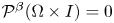 if $\beta >\beta _{0}$
 , then $\beta _{0}$
 is called as the parabolic Hausdorff dimension and $\mathcal {P}^{\beta }(\Omega \times I)$
 is the parabolic Hausdorff measure. The details of fractal dimension can be found in [Reference Falconer8].
Next, we focus on Caffarelli and Silvestre's generalized extension for the fractional Laplacian operator $(-\Delta )^{\alpha }$ with $0<\alpha <1$
 in [Reference Caffarelli and Silvestre5]. The fractional power of Laplacian in $\mathbb {R}^{3}$
 can be interpreted as

where $u^{\ast }$ satisfies

As a by-product of the above equation, for any $v |_{y=0}=u$ , it holds

Moreover, from § 3.2 in [Reference Caffarelli and Silvestre5], the definition of the $\dot {H}^{\alpha }$ norm can be written as

We recall the following observation due to [Reference Colombo, De Lellis and Massaccesi6], for $\alpha >1$ ,

Hence,

Based on the natural scaling of the Navier–Stokes equations, we set the following two dimensionless quantities:

To make our paper more self-contained and more readable, we outline the proof of the Poincaré inequality concerning Caffarelli and Silvestre's generalized extension.
Lemma 2.2 Let $u$ and $u^{\ast }$
 be defined in (2.1). There exist a constant $C$
 such that


Proof. Consider the usual cut-off functions

and

satisfying

By the Young inequalities, (2.3) and (2.2), we arrive at

This guarantees that

where $\overline {u^{\ast }}_{B^{\ast }(\mu )}=\frac {1}{|B^{\ast }(\mu )|} \int _{B^{\ast }(\mu )}y^{1-2s} u^{\ast }\,{\rm d}x\,{\rm d}y$ and $|B^{\ast }(\mu )|=\int _{B^{\ast }(\mu )} y^{1-2s}\,{\rm d}y\,{\rm d}x.$

Thanks to the classical weighted Poincaré inequality, we infer that

Plugging (2.8) into (2.7), we observe that

This together with the Sobolev embedding yields that

It follows from $u^{\ast } = u(x)+\int ^{y}_{0}\partial _{z}u^{\ast }\,{\rm d}z$ and the Hölder inequality that

Combining (2.9) with the latter inequality, we deduct that

Proposition 2.3 ([Reference He, Wang and Zhou11]) Let the pair $(u, \Pi )$ be a suitable weak solution to the 3D Navier–Stokes system (1.1) in $Q(1)$
 . There exists an absolute positive constant $\epsilon$
 depending only on $p$
 and $q$
 such that if the pair $(u,\Pi )$
 satisfies

for $1\leq 2/q+3/p <2, 1\leq p,\,q\leq \infty$ , then $u\in L^{\infty }(Q(1/2))$
 .
Proposition 2.4 ([Reference Wang, Wu and Zhou33]) Let the pair $(u, \Pi )$ be a suitable weak solution to the 3D Navier–Stokes system (1.1) in $Q(1)$
 . For any $\delta >0$
 , there exists an absolute positive constant $\epsilon$
 such that if $u$
 satisfies

then $u\in L^{\infty }(Q(1/16)).$
For the generalization of the $\epsilon$ -regularity criterion (2.12) at one scale without pressure, the reader may refer to recent work [Reference Kwon16] by Kwon. Next, we recall the Leibniz rule for fractional derivatives and product estimates for the fractional Laplacian.
Lemma 2.5 ([Reference Kenig, Ponce and Vega12]) Let $\alpha >0$ , $p\in (1,\infty )$
 and $p_{i}\in (1,\infty )$
 , $i=1,2,3,4.$
 Then there exists a positive constant $C$
 such that

and

where $\frac 1p=\frac {1}{p_{1}}+\frac {1}{p_{2}}=\frac {1}{p_{3}}+\frac {1}{p_{4}}$ .
For the convenience of readers, we present the known fractional Gagliardo–Nirenberg inequality at the end of this section.
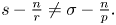
Proposition 2.6 ([Reference Hajaiej, Molinet, Ozawa and Wang10, Reference Wang, Mei and Wei32, Reference Wei, Wang and Ye34]) Suppose that $u\in L^{q}(\mathbb {R}^{n})$ and $\Lambda ^{s}u\in L^{r}(\mathbb {R}^{n})$
 . Let $0 \leq \sigma < s<\infty$
 and $1< q, r \leq \infty.$
 Then there exists a positive constant $C=C(n,q,p,r, s,\sigma )$
 such that

with

where $0 <\theta < 1-\frac {\sigma }{s}\,$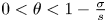 and $\,s-\frac {n}{r} \neq \sigma -\frac {n}{p}.$
3. Box dimension of possible singular points set of suitable weak solutions
This section contains the proof of theorem 1.1, corollary 1.3 and theorem 1.4. The key point is an application of the $\epsilon$ -regularity criteria (2.11) and (2.12) at one scale.
Proof of theorem 1.1. Proof of theorem 1.1
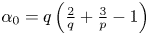
We present the proof by contradiction. We suppose that $\dim _{B}({\mathcal {S}})> \max \{p,q\}(\frac {2}{q}+\frac { 3}{p}-1).$ We pick a constant $\alpha$
 such that $\alpha _{0}=\max \{p,q\}\left (\frac {2}{q}+\frac {3}{p}-1\right )<\alpha <\dim _{B}({\mathcal {S}})$
 . Therefore, using the definition of the box dimension, we know that there exists a sequence $\delta _{j}\rightarrow 0$
 such that $N(\mathcal {S},\delta _{j})>\delta _{j}^{-\alpha }.$
 We assume that $(x_{i},t_{i})_{i=1}^{N(\mathcal {S},\delta _{j})}$
 be a collection of $\delta _{j}$
 - separated points in $\mathcal {S}$
 . By the regularity criterion in proposition 2.3, for any $(x_{i},t_{i})\in \mathcal {S}$
 , we get

where $B_{i}(\mu ):=B(x_{i}, \mu )$ . Thus we have

The pressure equation helps us to obtain, for $p>2$ , $q\geq 2$
 ,

For the case $\frac {q}{p}>1$ , we know that $\alpha _{0}=q\left (\frac {2}{q}+\frac {3}{p}-1\right )$
 .
Now, we can apply the inequality $\sum ^{N(\mathcal {S},\,{\delta _{j}})}_{i=1 } (a_{i})^{\frac {q}{p}}\leq (\sum ^{N(\mathcal {S},\,{\delta _{j}})}_{i=1 }a_{i})^{\frac {q}{p}}$ to control the left-hand side of (3.1) by $\|u\|^{q}_{L^{q}(0,T;L^{p}(\mathbb {R}^{3}))} +\|\Pi \|^{{q/2}}_{L^{q/2}(0,T;L^{p/2}(\mathbb {R}^{3}))}$
 . This together with (3.2) implies that

We immediately get a contradiction as $j\rightarrow \infty.$
For the rest case $\frac {q}{p}\leq 1$ , we invoke the inequality $\sum ^{N(\mathcal {S},\,{\delta _{j}})}_{i=1 } (a_{i})^{\frac {q}{p}}\leq N^{(1-\frac {q}{p})}(\mathcal {S},\,{\delta _{j}})(\sum ^{N(\mathcal {S},\,{\delta _{j}})}_{i=1 }a_{i})^{\frac {q}{p}}$
 in the proof. With a slight modification of the above proof, we see that $C \geq N^{\frac {q}{p}}(\mathcal {S},\,{\delta _{j}}) \delta _{j}^{(-p+3)\frac {q}{p}+2}\varepsilon _{1}$
 . This means that

This led a contradiction as $j\rightarrow \infty$ . The proof of this theorem is achieved.
Proof of corollary 1.3. Proof of corollary 1.3
It follows from $1\leq \frac {2}{q}+\frac { 3}{p}\leq \frac 32$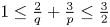 with $\frac 2p+\frac 2q<1$
 and $\frac 3p+\frac 1q<1$
 that $u\in L^{4}(0,T;L^{4}(\mathbb {R}^{n}))$
 . Thanks to the work [Reference Taniuchi28], we observe that $u$
 is a suitable weak solution. Following the path of the above proof, we complete the proof.
4. Hausdorff dimension of possible singular points set of suitable weak solutions
First, we prove proposition 1.6. As an application of this proposition, we can achieve the proof of corollary 1.7. To this end, we prove the following lemma, which roughly indicates that the smallness of $\nabla ^{\ast } (\nabla u)^{\ast }$ yields the smallness of $\nabla u$
 .
Lemma 4.1 For $0<\mu \leq \frac {1}{2}\rho$ , there is an absolute constant $C$
 independent of $\mu$
 and $\rho$
 , such that

Proof. With the help of the triangle inequality, the Hölder inequality and (2.6), we see that

that is,

Integrating in time on $({-\mu ^{2}},\,0)$ this inequality, we obtain

which leads to

This achieves the proof of this lemma.
Proof of proposition 1.6. Proof of proposition 1.6
From (1.12), we know that there exists a constant $\rho _{1}$ such that

Combining this with lemma 4.1, we conclude that, for $0<\rho \leq \rho _{1}$ ,

Before going further, we set $\lambda =\frac {\mu }{\rho }\leq \frac 12$ . Hence, there holds

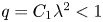
Choosing $\lambda$ sufficiently small such that $q=C_{1}\lambda ^{2}<1$
 and taking $\epsilon _{01}$
 such that $C_{1}\lambda ^{-1} \epsilon _{01}\leq \frac {(1-q)\epsilon \lambda }{2 }$
 , we obtain

Iterating this inequality, we infer that

Based on the definition of $E_{\ast }(\nabla u; \rho )$ , there is a positive sufficiently large number $K_{0}$
 such that

We write $\rho _{2}=\lambda ^{K_{0}}\rho _{1}$ , then, for all $0<\rho \leq \rho _{2}$
 , there is a positive constant $k\geq K_{0}$
 such that $\lambda ^{k+1}\rho _{1}\leq \rho \leq {\lambda ^{k}\rho _{1}}$
 and

where (4.2) and (4.3) were used.
Finally, the famous $\epsilon$ -regularity criterion (1.2) helps us to finish the proof of this proposition.
Now we are in a position to complete the proof of theorem 1.5.
Proof of theorem 1.5. Proof of theorem 1.5
For the case $s=0$ , we complete the proof by the Caffarelli–Kohn–Nirenberg theorem in [Reference Caffarelli, Kohn and Nirenberg4]. For the other borderline case $s=1/2$
 , by the fact $\dot {H}^{\frac 32}(\mathbb {R}^{3})\hookrightarrow BMO$
 and the Serrin class $L^{2}(0,T;BMO)$
 due to Kozono and Taniuchi [Reference Kozono and Taniuchi13], we know there is no singular point in the weak solutions of the Navier–Stokes equations. Hence, we achieve the proof of two borderline cases. For the rest cases, from (2.4), we derive from $u\in L^{2}(0,T;\dot {H}^{s+1}(\mathbb {R}^{3}))$
 with $0< s<\frac 12$
 that

At this stage, the Vitali covering lemma used in [Reference Caffarelli, Kohn and Nirenberg4] together with proposition 1.6 yields that $1-2 s$ dimension of potential singular points set of suitable weak solutions satisfying $u\in L^{2}(0,T;\dot {H}^{s+1}(\mathbb {R}^{3}))$
 for $0< s <\frac 12$
 is zero. The process is standard, hence, we omit the detail here.
In summary, the desired result is derived.
The proof of corollary 1.7 is a consequence of the following two lemmas.
Lemma 4.2 Let $\nabla u\in L^{q}(0,T;L^{p}(\mathbb {R}^{3}))$ for $2\leq \frac {2}{q}+\frac { 3}{p}\leq \frac 52$
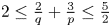 with $\frac 52-\frac 3p-\frac {5}{2q}\geq 0, 2< p<\frac {54+12\sqrt {14}}{25},{1< q\leq 2}$
 . Then

where $0\leq s=\frac {\frac 52-\frac 3p-\frac {5}{2q}}{1-\frac 1q}{\leq \frac {1}{2}}$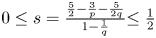 .
Proof. The incompressible condition allow us to get

Multiplying the Navier–Stokes equations with $\Lambda ^{2s}u$ , using the divergence-free condition and (4.4), we know that

The Hölder inequality guarantees that

By means of the Leibniz rule for fractional derivatives (2.13), we infer that

Consequently, we arrive at

We conclude by the fractional Gagliardo–Nirenberg inequality (2.15) and the Sobolev inequality that,

where we require

Indeed, in the light of the definition of $s$ and $1< q\leq 2$
 , we observe that $\frac {\frac {3}{p}}{\frac 52-s-\frac 3p}\leq 1$
 . In addition, taking advantage of the definition of $s$
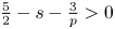
 again, we know that $\frac 52-s-\frac 3p>0$
 . Some straightforward computations yield that $\frac {9-\sqrt {56}}{6}<\frac 1p<\frac {9+\sqrt {56}}{6}$
 guarantees that $s\leq \frac {\frac {3}{p}}{\frac {5}{2}-s-\frac 3p}$
 .
Inserting (4.6) into (4.5), we have

Thanks to $\frac { \frac 52-s-\frac 6p}{\frac 52-s-\frac 3p}\leq 1$ , we derive from (4.7) and $\nabla u\in L^{q}(0,T;L^{p}(\mathbb {R}^{3}))$
 for $2\leq \frac {2}{q}+\frac { 3}{p}\leq \frac 52$
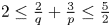 that $u\in L^{2}(0,T;\dot {H}^{1+s}(\mathbb {R}^{3}))$
 .
Lemma 4.3 Let $u$ be a suitable weak solution belonging to $\nabla u\in L^{q}(0,T;L^{p}(\mathbb {R}^{3}))$
 for $2\leq \frac {2}{q}+\frac { 3}{p}\leq \frac 52$
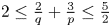 with $2-\frac 3p-\frac 1q\geq 0,\frac 32< p<\frac {12}{7},q\geq 4$
 . Then

where ${0\leq }s=\frac {2-\frac 3p-\frac 1q}{\frac 2q}{\leq \frac {1}{2}}$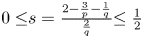 .
Proof. In view of the standard energy estimate, the integration by parts and the incompressible condition, we have

It follows from the Hölder inequality that

We deduce from the product estimates for the fractional Laplacian (2.14) and the Sobolev embedding that

Combining the above estimates together, we observe that

According to the fractional Gagliardo–Nirenberg inequality (2.15) and the Sobolev inequality, we discover that

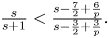
where we need $p\geq \frac 32,0\leq \frac {s-\frac 72+\frac 6p}{s-\frac 32+\frac 3p}\leq 1$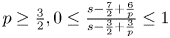 , $s-\frac 32+\frac 3p>0$
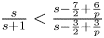
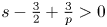 and $\frac {s}{s+1}<\frac {s-\frac 72+\frac 6p}{s-\frac 32+\frac 3p}$
 .
On one hand, we can examine $\frac {2-\frac 3p}{s-\frac 32+\frac 3p}\leq 1$ via $q\geq 4$
 and $2>p\geq \frac 32$
 . On the other, direct calculation ensures that $q>2, p>\frac 32$
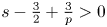
 yields that $s-\frac 32+\frac 3p>0$
 . Moreover, $\frac 32< p<\frac {12}{7}$
 means $\frac {s}{s+1}<\frac {s-\frac 72+\frac 6p}{s-\frac 32+\frac 3p}.$
Inserting (4.9) into (4.8), we find

which implies that

We deduce from $p>\frac 32$ that $\frac { s-\frac 72+\frac 6p}{s-\frac 32+\frac 3p}+1<2$
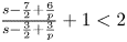 . Hence, the Young inequality further allows us to get that

The proof of this lemma is completed.
Acknowledgements
The authors express their sincere gratitude to Dr. Wei Wei at Northwest University, for the discussion involving the inequalities (4.6) and (4.9). The research of Wang was partially supported by the National Natural Science Foundation of China (Nos. 11971446 and 11601492) and sponsored by Natural Science Foundation of Henan (No. 232300421077). The research of Wu was partially supported by the National Natural Science Foundation of China under Grant No. 11771423.



