1. Introduction
Tubercles are rounded leading edge protuberances that alter the flow field around a foil. It has been suggested that tubercles on the humpback whale flipper function as lift enhancement devices, allowing flow to remain attached for a larger range of attack angles, thus delaying stall and increasing the maximum lift coefficient with minimal drag penalties (Miklosovic et al. Reference Miklosovic, Murray, Howle and Fish2004). This improved performance has been demonstrated both experimentally and numerically (Watts & Fish Reference Watts and Fish2001; Miklosovic et al. Reference Miklosovic, Murray, Howle and Fish2004; Pedro & Kobayashi Reference Pedro and Kobayashi2008).
A number of explanations for the observed performance enhancement have been proposed, which include increased boundary-layer momentum exchange (Fish & Battle Reference Fish and Battle1995; Miklosovic et al. Reference Miklosovic, Murray, Howle and Fish2004; Custodio Reference Custodio2007; Johari et al. Reference Johari, Henoch, Custodio and Levshin2007; Pedro & Kobayashi Reference Pedro and Kobayashi2008), compartmentalisation of the flow and subsequent minimisation of tip stall (Fish & Battle Reference Fish and Battle1995; Stein & Murray Reference Stein and Murray2005; Miklosovic & Murray Reference Miklosovic and Murray2007; Pedro & Kobayashi Reference Pedro and Kobayashi2008), non-uniform separation characteristics (Fish & Lauder Reference Fish and Lauder2006; Johari et al. Reference Johari, Henoch, Custodio and Levshin2007; van Nierop, Alben & Brenner Reference van Nierop, Alben and Brenner2008; Pedro & Kobayashi Reference Pedro and Kobayashi2008), alteration of the pressure distribution over the foil surface (van Nierop et al. Reference van Nierop, Alben and Brenner2008) and vortex lift (Custodio Reference Custodio2007; Miklosovic & Murray Reference Miklosovic and Murray2007). The different explanations for performance enhancement may arise from variations in the Reynolds number, aspect ratio, wing tip condition, sweep, taper and tubercle geometry. A more detailed literature review on the effect of these parameters can be found in Hansen (Reference Hansen2012), but here the discussion will be limited to the effect of the tubercle geometry.
According to a parametric study carried out by Favier, Pinelli & Piomelli (Reference Favier, Pinelli and Piomelli2012), variation of the amplitude and wavelength of tubercles affects the wake topology, the size of the recirculation zone and the strength of the wake vortex shedding. These researchers investigated a deep stall condition with an angle of attack of
 ${\it\alpha}=20^{\circ }$
and a low Reynolds number of
 $Re=800$
. It was shown that for amplitude to chord ratios
 $A/c<0.07$
, the intensity of the vortices is too weak to stabilise the separation region. For
 $A/c\geqslant 0.07$
, the frequency spectrum was observed to flatten, indicating a weakening of the wake vortex shedding. The wavelength between tubercles was found to influence the separation characteristics, where the flow was fully separated for
 $A/c=0.07,{\it\lambda}/c=0.5$
but attached behind the peaks for
 $A/c=0.07,{\it\lambda}/c=1$
. A parametric study was also performed by Johari et al. (Reference Johari, Henoch, Custodio and Levshin2007), and it was highlighted that the maximum lift coefficient, highest stall angle and minimum drag were achieved by the tubercle configuration with the smallest amplitude and smallest wavelength of tubercles (
 $A/c=0.025,{\it\lambda}/c=0.25$
). On the other hand, the tubercle configuration with the largest-amplitude tubercles (
 $A/c=0.12$
) exhibited the most gradual stall. These findings were supported by Hansen, Kelso & Dally (Reference Hansen, Kelso and Dally2011), and it was shown that for a given amplitude to wavelength ratio,
 $A/{\it\lambda}$
, the maximum lift coefficient, highest stall angle and minimum drag were attained for the smallest amplitude and wavelength configuration (
 $A/c=0.029,{\it\lambda}/c=0.11$
). Flow visualisation results indicated that streamwise vortices were present for all tubercle configurations investigated, but the size of these structures increased with tubercle amplitude (Hansen Reference Hansen2012).
Previous studies have shown that streamwise vortices exist as counter-rotating pairs which are located in the troughs between tubercles (Custodio Reference Custodio2007; Stanway Reference Stanway2008; Hansen et al. Reference Hansen, Kelso and Dally2011). The existence of streamwise vortices is of importance since many of the proposed performance enhancement mechanisms can be explained with reference to this flow phenomenon. Various mechanisms have been proposed to be responsible for the generation of streamwise vorticity. Weber et al. (Reference Weber, Howle, Murray and Miklosovic2011) suggested that each tubercle can be modelled as a small delta wing with a rounded leading edge. For a delta wing, the flow separates from the leading edge as it passes from the pressure surface to the suction surface, leading to the formation of a pair of streamwise vortices (Andersen Reference Andersen2007). On the other hand, Favier et al. (Reference Favier, Pinelli and Piomelli2012) proposed that the generation of streamwise vortices is attributed to a Kelvin–Helmholtz instability which arises due to differences in flow velocities behind the tubercle peaks and troughs. It was suggested that this instability produces tubes of vorticity, aligned normal to the surface in the leading edge region, which are abruptly rotated into the streamwise direction as the vorticity is advected by the mean flow. The existence of surface normal vorticity was shown experimentally by Stanway (Reference Stanway2008) using particle image velocimetry (PIV). Pairs of vortical structures of opposite sign were identified in the regions downstream from each tubercle (Stanway Reference Stanway2008). These structures were found to strengthen with increasing angle of attack (Stanway Reference Stanway2008).
Considering the flow field to contain a series of counter-rotating streamwise vortices as observed by Weber et al. (Reference Weber, Howle, Murray and Miklosovic2011), it can be deduced that there is a net downwash at the tubercle peaks and a net upwash at the troughs. This is consistent with the results presented by van Nierop et al. (Reference van Nierop, Alben and Brenner2008), which show mathematically that the variation in chord and thickness for a foil with tubercles creates changes in the circulation with spanwise location. Consequently, a sheet of streamwise vortices is generated behind the wing, causing a higher relative downwash at the peaks relative to the troughs and a variation in the effective angle of attack with spanwise location (van Nierop et al. Reference van Nierop, Alben and Brenner2008). There is also a more severe pressure gradient behind the troughs, which leads to earlier separation compared with the peak regions (Johari et al. Reference Johari, Henoch, Custodio and Levshin2007; van Nierop et al. Reference van Nierop, Alben and Brenner2008; Weber et al. Reference Weber, Howle, Murray and Miklosovic2011). Moreover, the magnitude of the suction peak within the troughs is higher than that on the peaks for a given angle of attack, which leads to a spanwise variation in pressure (Skillen et al. Reference Skillen, Revell, Pinelli, Piomelli and Favier2014).
The strong spanwise pressure gradient near the leading edge is another important aspect of the flow physics specific to tubercles, which has been observed in several numerical simulations (Weber et al. Reference Weber, Howle, Murray and Miklosovic2011; Rostamzadeh et al. Reference Rostamzadeh, Kelso, Dally and Hansen2013; Skillen et al. Reference Skillen, Revell, Pinelli, Piomelli and Favier2014) and also experimentally using pressure taps (Hansen et al. Reference Hansen, Kelso and Dally2011; Rostamzadeh et al. Reference Rostamzadeh, Kelso, Dally and Hansen2013). According to Skillen et al. (Reference Skillen, Revell, Pinelli, Piomelli and Favier2014), this spanwise pressure gradient induces a secondary flow slightly aft of the leading edge whereby low-momentum boundary-layer fluid is transported in the spanwise direction from peak to trough. The low-inertia fluid which has been transported away from the peak location by this secondary flow is replaced by high-momentum fluid drawn from above. There is a corresponding delay in flow separation behind the tubercle peaks (Skillen et al. Reference Skillen, Revell, Pinelli, Piomelli and Favier2014). This mechanism is complemented by a lower effective angle of attack at the peak position, which also leads to greater flow attachment (van Nierop et al. Reference van Nierop, Alben and Brenner2008). Rostamzadeh et al. (Reference Rostamzadeh, Hansen, Kelso and Dally2014) identified that since the spanwise circulation varies along the span of the foil (van Nierop et al. Reference van Nierop, Alben and Brenner2008), the spanwise vorticity should also vary by virtue of Stokes’ law. The cyclic variation in spanwise vorticity was shown to lead to the development of pairs of counter-rotating streamwise vortices. Turning of the vortex lines from a spanwise-dominant orientation towards the streamwise and surface-normal directions was attributed to the development of Prandtl’s secondary flow of the first type. This mechanism is activated by the presence of skewness in the flow, arising from spanwise pressure gradients, and vorticity within the boundary layer (Rostamzadeh et al. Reference Rostamzadeh, Hansen, Kelso and Dally2014). The existence of surface-normal vorticity observed in the experiments by Stanway (Reference Stanway2008) is attributed to this mechanism rather than a Kelvin–Helmholtz instability as suggested by Favier et al. (Reference Favier, Pinelli and Piomelli2012).
Therefore, one of the aims of the present work is to investigate the nature, formation and development of streamwise vortices over the suction surface of a foil with tubercles in the laminar flow regime. This is facilitated by the analysis of PIV results to determine the velocity fields on a series of image planes positioned perpendicular to the mean flow. These image planes are located at different chordwise positions, allowing observation of the downstream development of the velocity field. This information enables the vorticity and circulation to be determined, thus facilitating identification of the streamwise vortices and quantification of their strength. The PIV investigation is complemented with a computational fluid dynamics (CFD) simulation, where the experimental conditions are matched as closely as possible. The CFD results provide a means of investigating the flow structure in greater depth to reveal the complex nature of the flow pattern and mechanisms of vorticity generation. The evolution of the flow pattern over time is also illustrated using hydrogen bubble visualisation, and the results support the observations made in the PIV and CFD investigations.
2. Experimental work
2.1. Equipment
Experiments were undertaken in a free-surface closed-return water channel at the University of Adelaide. The working section of this flow facility is
 $350~\text{mm}\times 500~\text{mm}$
and is made entirely of clear acrylic. A free-stream velocity of
 $U_{\infty }=32~\text{mm}~\text{s}^{-1}$
was selected for the PIV measurements as the lowest number of outliers (spurious velocity vectors) in the velocity-vector field was recorded at this velocity compared with higher free-stream velocities. This remained the case even when the timing between laser pulses was varied, since the flow structures moved relatively slowly at this velocity. At a free-stream velocity of
 $U_{\infty }=32~\text{mm}~\text{s}^{-1}$
, the Reynolds number based on the foil chord was
 $Re=2230$
and the measured turbulence intensity was approximately 1.7 % based on an ensemble average of 3845 image pairs.
The foil profile chosen for the experiments was the NACA 0021, since it resembles the cross-section of the humpback whale flipper (Miklosovic et al.
Reference Miklosovic, Murray, Howle and Fish2004). The mean foil chord length was
 $c=70~\text{mm}$
and the planform shape was rectangular. The foil was machined from aluminium on a numerically controlled milling machine, and in order to reduce laser reflections, it was anodised in matte black. It was mounted such that it extended from the water surface to within 1 mm of the channel floor to minimise three-dimensional effects. This is within the range of the suggested maximum gap of
 $0.005\times \text{span}$
(Barlow, Rae & Pope Reference Barlow, Rae and Pope1999).
Based on results from a study by Fish & Battle (Reference Fish and Battle1995), the average amplitude,
 $A$
, and wavelength,
 ${\it\lambda}$
, for tubercles on a humpback whale flipper are approximately
 $A=4~\text{mm}$
and
 ${\it\lambda}=30~\text{mm}$
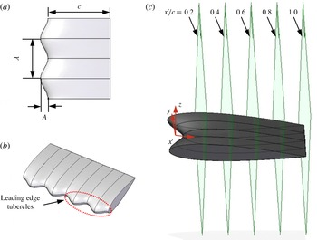
. However, to ensure that the vortex structures would be resolvable with sufficient accuracy, a larger amplitude was chosen compared with the average tubercle amplitude on the humpback whale flipper. Figure 1(a,b) shows the foil with tubercles, where the amplitude was selected to be
 $A=8~\text{mm}$
and the wavelength to be
 ${\it\lambda}=30~\text{mm}$
.
(a) Tubercle dimensions, (b) 3D view of foil section with tubercles, (c) foil section with tubercles showing PIV image planes.

This configuration was chosen based on the results of previous studies, which indicated that a larger amount of post-stall lift is achieved for larger-amplitude tubercles (Custodio Reference Custodio2007; Johari et al. Reference Johari, Henoch, Custodio and Levshin2007; van Nierop et al. Reference van Nierop, Alben and Brenner2008; Hansen et al. Reference Hansen, Kelso and Dally2011). If the streamwise vortices are either directly or indirectly responsible for this increased post-stall lift, it is implied that the strength and perhaps size of vortices for larger-amplitude tubercles is greater. An increase in the vortex intensity with tubercle amplitude has, in fact, been demonstrated by Favier et al. (Reference Favier, Pinelli and Piomelli2012), and flow visualisation results indicate that the size of the vortices increases with tubercle amplitude (Hansen Reference Hansen2012). Larger vortex structures with relatively high vorticity are desirable for PIV measurements as there is a corresponding improvement in the spatial resolution and signal-to-noise ratio of the results. Potential applications for larger-amplitude tubercles include wind turbines, where increased post-stall lift and more gradual stall characteristics would be beneficial, especially in light and variable conditions.
2.2. Hydrogen bubble visualisation
For the hydrogen bubble visualisation investigation, the foil was mounted vertically at an angle of attack of
 ${\it\alpha}=10^{\circ }$
. Streaklines of hydrogen bubbles were generated by passing a low current through a sinusoidally kinked platinum wire with a diameter of
 $40~{\rm\mu}\text{m}$
. The wire was mounted vertically and connected to electrodes which were wired to a power supply that supplied the current necessary for electrolysis. The mounts were constructed and positioned in such a way as to minimise interference with the flow. The flow was illuminated with a thin light sheet (
 ${\sim}10~\text{mm}$
thick) generated using an overhead projector that was partially covered, leaving a narrow slit. Images were digitally recorded via a Sony DCR-TRV900E Mini-DV video camera which was connected to a laptop computer.
The water channel velocity was selected to give optimum flow conditions for visualisation with the hydrogen bubble method. Thus, a velocity of
 $U_{\infty }=70~\text{mm}~\text{s}^{-1}$
was utilised, corresponding to a Reynolds number based on the foil chord length of
 $Re=4370$
. This Reynolds number is still in the laminar range and therefore the corresponding flow patterns would be consistent with the slightly lower Reynolds number of
 $Re=2230$
that was used in the PIV experiments.
2.3. Particle image velocimetry
A series of image planes at
 $x^{\prime }/c=0.2$
, 0.4, 0.6, 0.8 and 1 were used to observe the development of the streamwise vortices, as shown in figure 1(c). The
 $x$
–
 $y$
–
 $z$
coordinate system is also shown in the figure, and this remains stationary for the remainder of this paper. The
 $z$
-axis is perpendicular to both the
 ${\it\alpha}=0^{\circ }$
chordline and the trailing edge. The
 $x$
-axis is aligned with the chordline at
 ${\it\alpha}=0^{\circ }$
and the
 $x^{\prime }$
-axis follows the foil chord at all angles of attack and is related to the
 $x$
-axis by
 $x^{\prime }=x/\cos {\it\alpha}$
, since the foil is rotated about the trailing edge. While the foil is stationary and does not undergo any pitching motion, the angle between the
 $z$
-axis and the
 $x^{\prime }$
-axis is dependent on the angle of attack. The
 $y$
-axis is perpendicular to the chordline and parallel with the trailing edge. The origin is located at the trough location with respect to the span, at the mean chord location with respect to the chord and at the chord line with respect to the thickness. The experimental investigation considered angles of attack of
 ${\it\alpha}=5^{\circ }$
and 10°. The image plane at
 $x^{\prime }/c=0.2$
yielded successful results for
 ${\it\alpha}=10^{\circ }$
only, hence this plane is not considered for
 ${\it\alpha}=5^{\circ }$
.
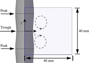
Since the pattern of the sinusoidal tubercles was periodic, it was not necessary to measure the velocity field for the entire foil span. Therefore, a compromise was made between resolving the flow patterns and ensuring that the area under investigation was sufficiently large to give an accurate representation of the overall flow behaviour. Based on these considerations, the field of view shown in figure 2 was chosen, giving an area of interest of
 $40~\text{mm}\times 40~\text{mm}$
and including two peaks and one trough. It was expected that the streamwise vortices would exist as counter-rotating pairs in each trough, as shown in figure 2. The measurement plane was located at the midspan of the foil to minimise end effects.
Typical field of view for PIV experiments (as seen by the camera), where the trailing edge and
 $x^{\prime }$
-axis point out of the page.

Velocity components in the plane shown in figure 2 were measured using two-component PIV. The flow was seeded with polyamide seeding particles (PSPs) which had a mean diameter of
 $d_{p}=50~{\rm\mu}\text{m}$
and a density of
 ${\it\rho}_{p}=1030~\text{kg}~\text{m}^{-3}$
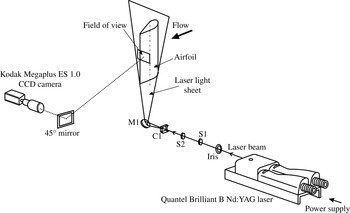
. Illumination was provided by a dual-cavity Quantel Brilliant B Nd:YAG laser. The wavelength of the laser light was 532 nm and the duration of each laser pulse was approximately 5 ns. From the laser beam, an optics train generated a 2 mm-thick light sheet. The optics set-up and camera positioning are shown in figure 3.
Optics set-up for PIV experiments (not to scale).

Particle image velocimetry images were recorded using a Kodak Megaplus ES 1.0 CCD camera with an array of
 $1008~\text{pixels}\times 1018~\text{pixels}$
and a Nikon 70–300 mm zoom lens. The image region of
 $40~\text{mm}\times 40~\text{mm}$
gave a spatial resolution of approximately
 $25~\text{pixels}~\text{mm}^{-1}$
. Particle image velocimetry image pairs were collected at a rate of 10 Hz, with the time delay between the laser pulses that illuminated the first and second images in each pair ranging from 20 to 32 ms. A Stanford DG535 pulse-delay generator regulated the triggering of the laser pulses from each laser cavity and enabled synchronisation with the recording system. XCAP-Plus software collected and transferred images to the computer hard disk as uncompressed 16-bit TIFF files. Particle image velocimetry velocity vectors were obtained by cross-correlation of the image pairs using the software package PivView v1.75. An interrogation window size of
 $32~\text{pixels}\times 32~\text{pixels}$
was used with 50 % overlap. Correlation peaks were detected using a multipass double-correlation least-squares Gaussian fit. Spurious velocity vectors or outliers were detected using a custom-written Matlab code which implemented the universal median technique described by Westerweel & Scarano (Reference Westerweel and Scarano2005).
To minimise uncertainties in the velocity-vector field, a total of 2085 image pairs were averaged temporally. Due to the large number of image pairs available, outliers detected using the normalised mean test (Westerweel & Scarano Reference Westerweel and Scarano2005) were not replaced and instead were omitted from the averaging process. For all averaged results presented in this paper, the number of outliers in a given velocity-vector field was less than 1 % of the total number of vectors. This confirms the validity of the measurements and verifies that out-of-plane particle motion had negligible effect on the results.
For the instantaneous results which were used to show time-dependent characteristics, detected outliers were replaced with a weighted average of valid surrounding vectors. Subsequently, an adaptive Gaussian window interpolator was implemented to reduce the amount of random noise associated with the velocity-vector field, as suggested by Agui & Jiminez (Reference Agui and Jiminez1987).
The average out-of-plane vorticity field,
 ${\it\omega}_{x}$
, was calculated from the in-plane velocity components using
 $$\begin{eqnarray}{\it\omega}_{x}=\frac{\partial w}{\partial y}-\frac{\partial v}{\partial z}.\end{eqnarray}$$
The chosen numerical scheme was the central difference scheme, which is adequate for most applications (Etebari & Vlachos Reference Etebari and Vlachos2005). Other schemes were considered but since the areas of interest were in close proximity to the boundaries of the velocity field, their large computational stencil caused inaccuracies.
The circulation,
 ${\it\Gamma}$
, of each vortex core was estimated by numerical integration based on the closed-curve line integral
 $$\begin{eqnarray}{\it\Gamma}_{vel}=\oint _{c}~(v\,\text{d}y+w\,\text{d}z),\end{eqnarray}$$
where
 $v$
is the component of velocity in the
 $y$
-direction and
 $w$
is the component of velocity in the
 $z$
-direction. The region enclosed by the path of integration encompassed the streamwise vortices and remained constant in area for each spanwise plane.
The random and bias uncertainties in particle displacement were calculated with reference to Willert & Gharib (Reference Willert and Gharib1991), Fouras & Soria (Reference Fouras and Soria1998), Hassan, Lau & Kelso (Reference Hassan, Lau and Kelso2007), Raffel, Willert & Kompenhans (Reference Raffel, Willert and Kompenhans2007) and Lau (Reference Lau2010). The overall uncertainty in vorticity for the averaged data was 1.4 % and the uncertainty in circulation was less than 1 %. The uncertainty analysis is discussed in further detail in appendix A.
3. Vorticity
A series of vorticity plots are shown in this section for angles of attack of
 ${\it\alpha}=5^{\circ }$
and
 ${\it\alpha}=10^{\circ }$
. In the vorticity plots, a counterclockwise sense of rotation is defined as positive (red) and a clockwise sense of rotation is defined as negative (blue). Images associated with each spanwise plane have been located adjacent to one another for comparison. Both the
 $y$
- and
 $z$
-axes have been made non-dimensional through dividing by the tubercle wavelength. The lower limit of the
 $z$
-axis values is governed by the foil curvature as well as the angle of attack, and hence is non-zero in most cases. For example, at
 $x^{\prime }/c=0.4$
and
 ${\it\alpha}=5^{\circ }$
, the distance in the
 $z$
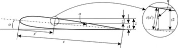
-direction between the origin and the foil surface can be calculated as
 $z_{surface}=10.7~\text{mm}$
, using the following equation:
 $$\begin{eqnarray}z_{surface}=(1-x^{\prime }/c)\times c\sin {\it\alpha}+t(x^{\prime })\times \cos {\it\alpha}.\end{eqnarray}$$
Here,
 $t(x)$
is the local thickness of the foil, which is evaluated at the point of interest. A schematic diagram is shown in figure 4 to illustrate the methodology used to derive equation (3.1). The corresponding non-dimensional value is
 $z/{\it\lambda}=0.36$
, which is close to the minimum value of the
 $z$
-axis in figure 5(a). Differences are due to the discretisation error associated with the size of the PIV interrogation windows.
Schematic diagram showing geometric quantities used to derive (3.1).

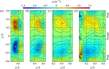
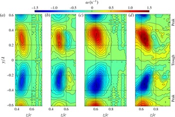
View of the vorticity field from behind the foil where the counterclockwise vortex core (red/upper) is positive and the clockwise vortex core (blue/lower) is negative. Angle of attack
 ${\it\alpha}=5^{\circ }$
,
 $Re=2230$
, image planes are shown for
 $x^{\prime }/c=0.4$
, 0.6, 0.8 and 1 (a–d).

Figure 5(a–d) shows that between tubercle peaks, there exist adjacent regions of positive (upper section) and negative (lower section) vorticity for all image planes. These regions of vorticity, marked ‘P’ in figure 5(a,b), will henceforth be described as the primary vorticity. With streamwise distance, vortex spreading leads to a decrease in the peak primary vorticity and an increase in the area over which vorticity is distributed. As shown in figure 5(a,b), vortex spreading is greater in the
 $y$
-direction than the
 $z$
-direction, where it is inhibited due to adjacent vorticity of opposite sign.
This vorticity of opposite sign (or secondary vorticity) has been marked with an asterix and is evident in the image planes of
 $x^{\prime }/c=0.4$
and
 $x^{\prime }/c=0.6$
in figure 5(a,b). This vorticity appears to be annihilated by the primary vorticity of opposite sign adjacent to it, as evidenced by its absence for image planes further aft. The process of annihilation is further evidenced by the closely spaced contours of vorticity between the primary and secondary structures in figure 5(a,b).
The asymmetrical appearance of figure 5(d) is consistent with the occurrence of unsteady effects at
 $x^{\prime }/c=1$
, which will be discussed in § 8. The asymmetry can also be attributed to possible differences in the flow patterns for adjacent wavelengths of the tubercle pattern. Flow visualisation images have shown that differences in the flow patterns exist for adjacent wavelengths of the tubercle pattern, but that alternate wavelengths demonstrate similar characteristics (Custodio Reference Custodio2007).
Another important feature that is visible in figure 5(d) is the existence of wall vorticity which is adjacent to the primary vortices and has an opposite sense of rotation. This wall vorticity is evident in the streamwise vorticity plots published by Skillen et al. (Reference Skillen, Revell, Pinelli, Piomelli and Favier2014), both at similar chordwise locations and at chordwise locations closer to the leading edge. The absence of wall vorticity near the leading edge for the PIV measurements reported here is due to resolution limitations.
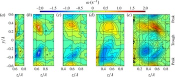
Figure 6 shows that increasing the foil angle of attack to
 ${\it\alpha}=10^{\circ }$
gives rise to an increase in the magnitude of the peak vorticity associated with the counter-rotating primary vortices. Consistent with the results at
 ${\it\alpha}=5^{\circ }$
, vortex spreading occurs in the streamwise direction at
 ${\it\alpha}=10^{\circ }$
, and the spreading of vorticity is restricted in the
 $z$
-direction at
 $x^{\prime }/c=0.2$
and 0.4 due to the proximity of secondary vorticity of opposite sign. Flow asymmetry is evident in the results at
 ${\it\alpha}=10^{\circ }$
for the image planes close to the trailing edge, as was observed for
 ${\it\alpha}=5^{\circ }$
, and is attributed to the same mechanism.
View of vorticity field from behind the foil where the counterclockwise vortex core (red/upper) is positive and the clockwise vortex core (blue/lower) is negative. Angle of attack
 ${\it\alpha}=10^{\circ }$
,
 $Re=2230$
, image planes are shown for
 $x^{\prime }/c=0.2$
, 0.4, 0.6, 0.8 and 1 (a–e).

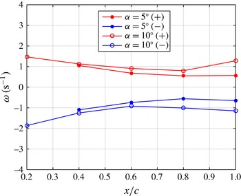
Magnitudes of the maximum positive and negative vorticity peaks for
 ${\it\alpha}=5^{\circ }$
and
 ${\it\alpha}=10^{\circ },Re=2230$
.

Figure 7 shows the magnitudes of the positive and negative primary vortex peaks corresponding to the contour plots shown in figures 5 and 6. The magnitudes of both vorticity peaks decrease with downstream distance for the image planes nearer to the leading edge (
 $x^{\prime }/c=0.2$
–
 $0.6$
) at
 ${\it\alpha}=5^{\circ }$
and
 ${\it\alpha}=10^{\circ }$
. In accordance with Morton (Reference Morton1984), the presence of strong pressure gradients near a foil leading edge results in the production of vorticity, giving rise to large values of the vorticity field in this region. This vorticity is, then, transported through viscous diffusion as well as the vortex stretching and tilting phenomena into the flow field. With the presence of large velocity gradients, in particular near the leading edge, the mechanism for the decay of peak vorticity is activated, as reflected in figure 7. Axial compression of streamwise vortices caused by the presence of an adverse pressure gradient on the suction surface of the foil leads to an increase in the cross-sectional area of the vortices, as shown in figures 5 and 6, and a corresponding reduction in the peak vorticity. The reduction in peak vorticity is also influenced by annihilation of the secondary vorticity, observed in figures 5(a,b) and 6(a,b), as well as diffusion and annihilation between the streamwise vortices themselves. Towards the trailing edge, the magnitude of the peak vorticity increases as a result of the vortex tilting phenomenon, as will be discussed in § 7.
4. Circulation of streamwise vortices
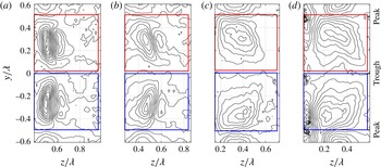
The integration paths for calculating the counterclockwise and clockwise circulation are shown superimposed on the vorticity contour plots for
 ${\it\alpha}=5^{\circ }$
in figure 8(a–d). The vorticity plots are shown with the same resolution as in figure 5, where the increment between contour lines is 0.1
 $\text{s}^{-1}$
. The corresponding regions enclosed by the integration paths are of equal size and the left-hand border of each plot aligns with the foil surface. This ensures that all significant vorticity contributions are captured within the integral as
 $x^{\prime }/c$
changes. Extending the right-hand border of these regions has negligible impact on the results. The regions of integration for an angle of attack of
 ${\it\alpha}=10^{\circ }$
are not shown for the sake of brevity.
Path of integration and enclosed region for
 ${\it\alpha}=5^{\circ }$
,
 $Re=2230$
, image planes
 $x^{\prime }/c=0.4$
, 0.6, 0.8 and 1 (a–d). Red/upper, integration path for calculating the circulation of the counterclockwise vortex; blue/lower, integration path for calculating the circulation of the clockwise vortex. The vorticity contours are plotted with the same resolution as figure 5, where the separation between contour lines is 0.1
 $\text{s}^{-1}$
.

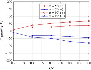
Circulation variation,
 ${\it\Gamma}$
, with angle of attack and chordwise position.

Results from the integration for
 ${\it\alpha}=5^{\circ }$
and
 ${\it\alpha}=10^{\circ }$
are depicted in figure 9, where the magnitude of the circulation is shown for both the positive and negative primary vortex cores. The circulation of the clockwise and anticlockwise primary vortices increases both with increasing angle of attack and with streamwise distance from the leading edge. These results were also observed when the region of integration encompassed the primary vorticity only, indicating that the secondary vorticity and wall vorticity have negligible impact on the magnitude of the circulation. To understand the reason behind the increase in circulation, it is first necessary to analyse the flow pattern in detail, and this will be done in § 7. Subsequently, the streamwise increase in circulation will be explained with reference to the identified flow mechanism.
Figure 9 shows that the circulation of the negative vortex is slightly higher than that of the positive vortex for the image planes at
 $x^{\prime }/c=0.8$
and
 $x^{\prime }/c=1$
at
 ${\it\alpha}=10^{\circ }$
. This is related to the asymmetry of the primary vortices which is apparent in figures 6(d) and 6(e).
A streamwise increase in circulation of the primary vortices has also been observed for delta wings prior to the point at which vortex breakdown occurs (Visser & Nelson Reference Visser and Nelson1993; Johari & Moreira Reference Johari and Moreira1998). The chord Reynolds numbers investigated were
 $Re=1.9\times 10^{\text{5}}$
and
 $Re=2.5\times 10^{\text{5}}$
, and the circulation increase was approximately linear. An approximately linear increase in circulation is also evident in figure 9.
5. Computational fluid dynamics model
ANSYS (2014) was employed to model the flow over the full-span tubercled and baseline NACA 0021 foils at
 $Re=2230$
for the two attack angles described in the experiments (
 ${\it\alpha}=5^{\circ }$
and
 ${\it\alpha}=10^{\circ }$
). To this end, the transitional shear stress transport (SST) model
 ${\it\gamma}$
–
 $Re_{{\it\theta}}$
(Langtry & Menter Reference Langtry and Menter2009), was used for solving the steady Reynolds-averaged Navier–Stokes equations. Here,
 ${\it\gamma}$
is defined as the intermittency, which determines the percentage of time that the flow is turbulent, and
 $Re_{{\it\theta}}$
is the momentum thickness Reynolds number. The
 ${\it\gamma}$
–
 $Re_{{\it\theta}}$
model was successful in capturing the pressure distribution and flow characteristics, including the vorticity field around a wavy foil, in our previous study (Rostamzadeh et al.
Reference Rostamzadeh, Kelso, Dally and Hansen2012).
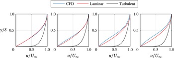
Boundary-layer plots for CFD results at an angle of attack of
 ${\it\alpha}=10^{\circ }$
for the foil cross-section corresponding to the tubercle peak, for (a)
 $x^{\prime }/c=0.0924$
, (b)
 $x^{\prime }/c=0.216$
, (c)
 $x^{\prime }/c=0.3329$
and (d)
 $x^{\prime }/c=0.4604$
.

The boundary-layer profile for the CFD results at
 ${\it\alpha}=10^{\circ }$
is shown in figure 10 for a series of spanwise planes at the peak cross-section. The parabolic flat-plate approximation to the laminar boundary-layer profile and the turbulent flat-plate approximation,
 $u/U_{\infty }=(y/{\it\delta})^{1/7}$
, are also shown for comparison. It can be seen that the boundary layer in the CFD results most closely resembles a laminar profile. This was also found to be the case at the trough and mid cross-sections. This supports the choice of the transitional SST model, since a laminar boundary layer would be expected at the low Reynolds number investigated in this study, and a transitional model allows specification of the free-stream turbulence intensity. Initially, a laminar model was implemented, but it was found that this model did not resolve the streamwise vortices correctly, leading to discrepancies between the computational and experimental results.
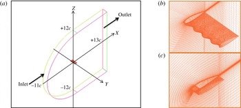
(a) The computational domain with the coordinate system positioned at the leading edge. (b,c) The grid system in the vicinity of the tubercled foil (b) and unmodified NACA 0021 foil (c).

To discretise the transport equations, ANSYS CFX 14.5 uses an element-based finite volume method (ANSYS 2014). High-resolution algorithms were implemented for the advection and turbulence numerical schemes. A C-grid topology with hexahedral elements was adopted as the computational domain, with far-field boundaries located at 12 chord lengths from the trailing edges of the foils, as shown in figure 11. The angle of attack was changed by rotating the model and maintaining constant values for the free-stream velocity components. The surfaces of the foils were assigned the no-slip boundary condition, and periodic conditions were applied to the side planes.
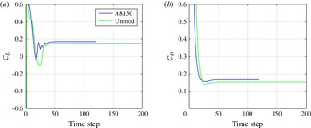
Force monitor plots for (a) the lift coefficient,
 $C_{L}$
, and (b) the drag coefficient,
 $C_{D}$
, for
 ${\it\alpha}=10^{\circ }$
.

As flow separation was expected to occur, the boundary layer had to be resolved with sufficient detail, hence the grid was refined near the wall boundaries such that
 $y^{+}<1$
. To assess convergence, the behaviour of the force monitor points was considered (see figure 12) along with a residual target equal to
 $10^{-7}$
for the momentum and SST transport equations, and
 $1.15\times 10^{-6}$
for the intermittency transport equation. The force monitor points are the lift coefficient,
 $C_{L}$
, and the drag coefficient,
 $C_{D}$
.
The geometric and the grid characteristics associated with the foils are provided in table 1. Although the mesh sensitivity analysis showed no difference in the behaviour of the forces with a lower-density grid test case (total number of hexahedral elements equal to 2859 012) for the tubercled foil, the adopted grid for simulation was capable of showing finer details of the vorticity field near the foil surface, which was of particular interest in this study. The flow mechanism described in this work was consistently detected across all of the test cases, including one with a much higher number of elements (10 748 400).
Grid and geometric details of the modelled foils.

Vorticity at
 $Re=2230$
, image plane
 $x^{\prime }/c=0.4$
, for (a)
 ${\it\alpha}=5^{\circ }$
(CFD), (b)
 ${\it\alpha}=5^{\circ }$
(experiment), (c)
 ${\it\alpha}=10^{\circ }$
(CFD), (d)
 ${\it\alpha}=10^{\circ }$
(experiment).

5.1. Validation
The computational model provides information that is not available from the described PIV experiment. However, to ensure that the CFD model accurately captures the flow physics, a series of comparisons were made with the PIV results. The image plane located at
 $x^{\prime }/c=0.4$
was used for this purpose as it was expected to have a lower associated unsteadiness, in which case averaging would yield more comparable results. The results for vorticity are shown in figure 13, where it can be seen that the magnitude and position of the peak vorticity are consistent for the experimental and numerical results for angles of attack of
 ${\it\alpha}=5^{\circ }$
and
 ${\it\alpha}=10^{\circ }$
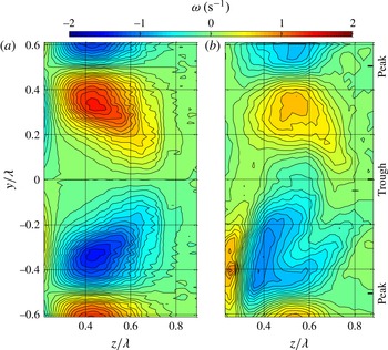
. Differences are apparent in the degree of vorticity spreading, where this is slightly greater for the numerical results shown in figures 13(a) and 13(c). In addition, the CFD technique does not predict the secondary vorticity, which was observed in the PIV experiments for image planes close to the leading edge.
Vorticity at
 $Re=2230$
, image plane
 $x^{\prime }/c=0.8$
, angle of attack
 ${\it\alpha}=10^{\circ }$
; (a) CFD, (b) experiment.

The CFD results shown in figure 14(a) reveal the presence of opposite-sign wall vorticity, which was also observed in the PIV experiments, as indicated in figure 14(b). Figure 14 also indicates that for the image plane at
 $x^{\prime }/c=0.8$
, CFD predicts a higher peak vorticity and the vortex cores are more symmetrical in comparison to the experimental results.
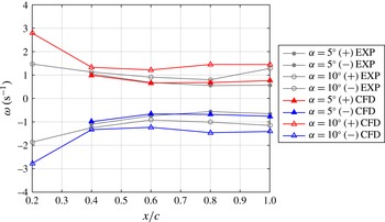
Experimental and numerical magnitude of peak positive and negative vorticity for
 ${\it\alpha}=5^{\circ }$
and
 ${\it\alpha}=10^{\circ },Re=2230$
.

Comparison between the magnitudes of the peak vorticity determined experimentally and numerically for the other chordwise positions is shown in figure 15. At an angle of attack of
 ${\it\alpha}=5^{\circ }$
, the magnitude of the peak vorticity is in good agreement for all spanwise planes. There is reasonable agreement between the results at
 ${\it\alpha}=10^{\circ }$
; however, the numerical results indicate a higher level of peak vorticity for all image planes. This is attributed to unsteady effects in the PIV experiments which give rise to attenuation of the time-averaged vorticity across the measurement plane, as will be discussed in § 8. Another notable difference between the experimental and numerical results is the magnitude of the peak vorticity for the image plane at
 $x^{\prime }/c=0.2$
. Since the vorticity for this particular plane is close to the wall, it may not have been captured in the experiments due to grid resolution limitations and, hence, the experimentally determined peak vorticity could be lower than the actual value. This is supported by the fact that the spanwise pressure gradient in the region upstream of
 $x^{\prime }/c=0.2$
is relatively high, as will be shown in § 6, and would thus contribute to the generation of streamwise vorticity at the surface in this region (Gad-el-Hak 2006).
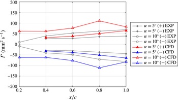
Experimental and numerical results showing the variation in circulation,
 ${\it\Gamma}$
, with angle of attack and chordwise position.

The circulation was calculated using the method described in § 2.3 for both the experimental and numerical cases and is shown in figure 16. The CFD results confirm that the circulation generally increases in the downstream direction for both
 ${\it\alpha}=5^{\circ }$
and
 ${\it\alpha}=10^{\circ }$
. Reasonable agreement was achieved between the circulation results for the various spanwise planes at an angle of attack of
 ${\it\alpha}=5^{\circ }$
. At the higher angle of attack of
 ${\it\alpha}=10^{\circ }$
, the circulation determined from CFD is greater than the value determined experimentally. Moreover, the CFD results indicate that the circulation decreases between the spanwise planes at
 $x^{\prime }/c=0.8$
and
 $x^{\prime }/c=1$
, rather than increasing as determined from the PIV experiments. One explanation for these differences may be that unsteadiness in the experimental flow leads to a variation in the positions and strengths of the vortical features, which is manifested as an attenuation of the time-averaged vorticity across the measurement plane, as suggested in § 8. The result of this phenomenon is a more gradual change in circulation with streamwise location. On the other hand, the differences in the experimental and numerical results may also be an effect of the CFD closure model, which influences the location of the separation lines.
6. Pressure forces
This section presents the chordwise pressure distributions corresponding to a tubercle peak, a trough and midway between. The data were obtained from the CFD simulation described in § 5. Analysis of the surface pressure distributions allows identification of the point at which the adverse pressure gradient initiates for each cross-section, which is relevant to the vortex stretching mechanism. The chordwise pressure distributions show the existence of a spanwise variation in pressure, and this is explored further through plotting surface contours of the spanwise pressure gradient. The spanwise pressure gradient is shown to result in the generation of streamwise vorticity at the surface. Analysis of the surface pressure data also enables investigation into the spanwise variation in lift.
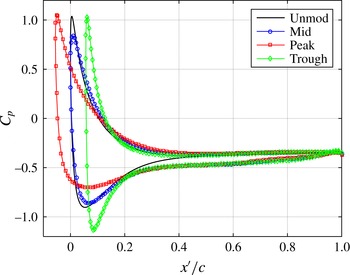
Pressure distribution for the unmodified (unmod) and tubercled foil at
 ${\it\alpha}=10^{\circ }$
, where ‘peak’, ‘trough’ and ‘mid’ correspond to the cross-sections at the tubercle peak, trough and midway between. Here,
 $C_{p}$
is the pressure coefficient.

The chordwise variation in pressure for both the unmodified and tubercled foils at
 ${\it\alpha}=10^{\circ }$
is shown in figure 17. The most negative values of the peak pressure developed over the suction surface of the tubercled foil are associated with the trough cross-section. The lowest minimum suction peak occurs at the peak cross-section, and the pressure values for the middle cross-section lie somewhere between. This is consistent with results obtained at a higher Reynolds number on a foil with the same profile shape (Hansen Reference Hansen2012). It must be noted that the slight overprediction in the pressure coefficient at the stagnation points is due to numerical error and was not resolved by refining the CFD grids or extending the domain boundaries up to 40 chord lengths. The impact of this error is negligible on the underlying flow mechanism reported in this work.
The location of the suction peak along the trough cross-section is further aft than for the other cross-sections and the unmodified foil. Conversely, the suction peak along the peak cross-section is slightly closer to the leading edge. This variation is attributed to differing positions of maximum thickness as well as changes in chord length with spanwise location. These parameters define the position at which the adverse pressure gradient initiates. At this point, compression of streamwise vortices is initiated, resulting in a larger area over which vorticity is distributed and a reduction in peak vorticity, as discussed in § 3.
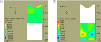
Spanwise pressure gradient on the surface of the foil at
 ${\it\alpha}=10^{\circ },Re=2230$
, where the highest values occur at the foil leading edge.

The difference in magnitude and location of the suction peaks for the mid, peak and trough cross-sections gives rise to a spanwise pressure gradient which initiates at the leading edge and persists up to approximately
 $x^{\prime }/c=0.2$
. The contour plot shown in figure 18 indicates the magnitude of the spanwise pressure gradient in the region of the leading edge. It is also evident that a spanwise pressure gradient exists near the trailing edge; however, its magnitude is significantly lower.
The presence of a spanwise pressure gradient results in direct production of streamwise vorticity, as can be seen by the spanwise momentum equation at the wall expressed in (6.1) (Gad-el-Hak 2006), where the coordinate axes are consistent with figure 1 in § 2,
 $$\begin{eqnarray}\left.{\it\rho}v_{w}\frac{\partial v}{\partial z}\right|_{z=0}+\left.\frac{\partial p}{\partial y}\right|_{z=0}-\left.\frac{\partial {\it\mu}}{\partial z}\frac{\partial v}{\partial z}\right|_{z=0}={\it\mu}\!\left.\frac{\partial ^{2}v}{\partial z^{2}}\right|_{z=0}.\end{eqnarray}$$
The first and third terms on the left-hand side of the equation are equal to zero due to the absence of flow injected from the wall,
 $v_{w}$
, and constant viscosity,
 ${\it\mu}$
. Therefore, the spanwise pressure gradient,
 $\partial p/\partial y$
, can be seen to affect the curvature of the velocity profile shown on the right-hand side of the equation, which is the same as the flux of streamwise vorticity from the wall (Gad-el-Hak 2006).
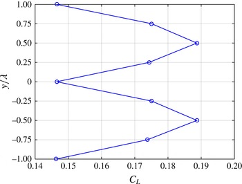
Variation in the lift coefficient,
 $C_{L}$
, with the spanwise location.

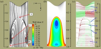
(a) Shear stress lines, (b) shear stress contours and (c) vortex lines,
 ${\it\alpha}=5^{\circ },Re=2230$
.

Lift and drag forces at
 ${\it\alpha}=10^{\circ }$
calculated in the CFD simulation.

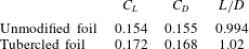
Results from the CFD simulation shown in table 2 indicate that the lift coefficient achieved by the foil with tubercles is higher than that achieved by the unmodified foil. In addition, the efficiency of the tubercled foil,
 $L/D$
, is marginally better than that of the unmodified foil, despite the slight increase in the associated drag. The increased lift for the tubercled foil is attributed to the greater flow attachment that is maintained behind the tubercle peaks. Integration of the pressure at the peak, trough and midway between (mid) cross-sections confirms that the highest proportion of lift is generated at the peak cross-section, as shown in figure 19. The spanwise variation in the circulation and hence lift coefficient is also highlighted in figure 19. The increased drag for the foil with tubercles is related to the presence of streamwise vortices and the associated increase in surface shear stress.
7. Analysis of flow characteristics
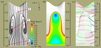
Regions of separation and attachment of the flow on the foil can be identified from the surface shear stress lines and contours shown in figures 20(a,b) and 21(a,b). These images were obtained from the CFD simulation described in § 5. Behind the tubercle trough, separation occurs much earlier than behind the peak, which is consistent with previous results (Johari et al. Reference Johari, Henoch, Custodio and Levshin2007; van Nierop et al. Reference van Nierop, Alben and Brenner2008). The surface shear stress lines show that a large separation zone forms ahead of a pair of foci (F), into which the flow spirals, to be lifted from the surface. The upstream extent of the separation zone is defined by a saddle point (S).
The foci mark the locations at which concentrated vortices separate from the surface of the foil, which occurs at
 $x^{\prime }/c\sim 0.8$
and
 $x^{\prime }/c\sim 0.6$
for
 ${\it\alpha}=5^{\circ }$
and
 ${\it\alpha}=10^{\circ }$
respectively. Downstream of the foci, aligned with the tubercle peaks, lie a pair of bifurcation lines (BL) which define the spanwise extent of the separation zone. In the following discussion we will describe the downstream evolution of both surface vorticity and vorticity in the separated shear layer. This analysis provides insight into the mechanisms responsible for the presence of streamwise vorticity in the numerical and experimental results and how these may explain the experimental observations of streamwise vorticity at various spanwise planes above the foil.
(a) Shear stress lines, (b) shear stress contours and (c) vortex lines,
 ${\it\alpha}=10^{\circ },Re=2230$
.

The evolution of the vorticity vectors over the foil surface is shown by the vortex lines in figures 20(c) and 21(c). In these figures, vortex lines are coloured according to the sign of the streamwise vorticity, where red (darker) and green (lighter) are positive and negative respectively, in the
 $x^{\prime }$
-direction. For a conventional unswept foil without tubercles, vortex lines are initially aligned in the
 $y$
-direction, parallel to the leading edge, with positive vorticity, consistent with the mean shear. However, in the highly three-dimensional flow around the tubercles, the vortex lines are initially wavy, leading to streamwise vorticity components on the sides (A) of the tubercles themselves. A short distance downstream, the curvature becomes reversed (B) ahead of the separation zone, leading to small streamwise vorticity components of opposite sign to the streamwise vorticity on the tubercles.
Downstream of the saddle the vortex lines can be seen to bend sharply downstream (C), merging into a single line (M), representing the edge of the canopy-like separated vortex sheet that defines the separation zone. The edge of the canopy is also indicated in the associated surface shear stress contours. The downstream orientation of the vortex lines near the foil surface (C) leads to additional streamwise vorticity of the same sign as the primary vortices formed on the sides of the tubercles. In both figures 20 and 21 the vortex lines are seen to be turned over the entire length of the separation zone, supporting the observation that the circulation of the streamwise vortices formed adjacent to the separation zone increases with downstream distance, as shown in § 4.
In figures 20(c) and 21(c) the vortex lines in the reversed flow region, which are of opposite sign to those of the upstream boundary layer, are also seen to contribute to the generation of streamwise vorticity components (D) upstream of the foci. However, downstream of the foci, the vortex line curvature is reversed (E), leading to vorticity of a sign opposite to the primary vortices. The presence of strong streamwise vorticity of opposite sign beneath the primary vortices is confirmed by the experimental and numerical results for the
 ${\it\alpha}=10^{\circ }$
case in figure 14. Finally, the vortex lines near the trailing edge (F) at
 ${\it\alpha}=10^{\circ }$
in figure 21 are orientated such that the streamwise vorticity is of the same sign as observed at (C).
Magnitude of the vortex turning terms for
 ${\it\alpha}=10^{\circ },Re=2230$
, in the vicinity of (a) the leading edge and (b) the trailing edge.

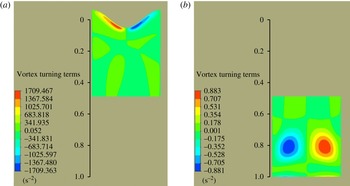
The turning of the surface vortex lines from a spanwise-dominant orientation towards the streamwise direction is caused by the deflection or skewing of the mean flow, which is described by the term
 ${\it\omega}_{y}(\partial u/\partial y)+{\it\omega}_{z}(\partial u/\partial z)$
in the vorticity transport equation (Perkins Reference Perkins1970). The magnitude of the vortex turning terms is shown to be largest in the region of the leading edge in figure 22(a). Near the trailing edge, after
 $x^{\prime }/c=0.6$
, the sign of the vortex turning terms changes, as shown in figure 22(b), which is consistent with the reversal of the vortex line curvature that occurs in this region. Direct generation of streamwise vorticity also occurs in both of these regions, as was discussed in § 6.
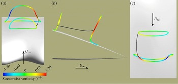
(a) Three-dimensional vortex line interpretation, (b) vortex lines from CFD simulation and (c) vortex lines with normalised green (lighter) and red (darker) arrows indicating spanwise and streamwise orientation of vorticity respectively.

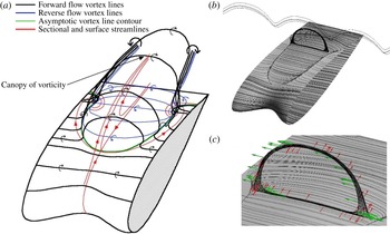
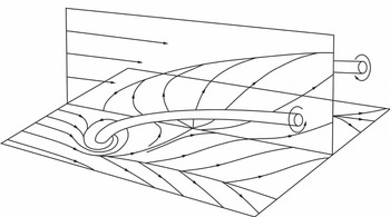
A three-dimensional vortex line interpretation is shown in figure 23(a) to provide a more detailed visualisation of the proposed flow mechanism. Along the asymptotic vortex line contour, the vortex lines lift from the foil surface, forming a canopy of vorticity above the separation zone. At the edge of the canopy-shaped vortex sheet, the forward flow and reverse flow vortex lines contribute to streamwise vorticity of the same sign, referred to as ‘primary vorticity’ in this study. This process occurs continuously along the sides of the canopy, consistent with the growth of the circulation of the primary vortices with streamwise distance (see figure 16).
A pair of foci is revealed by the surface streamlines in figure 23(a), and the primary vortices separate from the surface at these points. The vortex lines corresponding to the CFD results are shown in figure 23(b), and these results support the vortex line interpretation and show the canopy of vorticity that forms in the separation region aft of the tubercle troughs. The sign of vorticity on the vortex line ring is indicated in figure 23(c), and it is emphasised that this is different from the boundary-layer vorticity shown in figure 23(a).
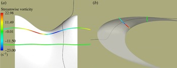
(a) Three-dimensional vortex lines coloured by streamwise vorticity in the vicinity of
 $x^{\prime }/c=0.6$
and
 $x^{\prime }/c=0.8,{\it\alpha}=10^{\circ }$
. (a) Three-dimensional view, (b) side view and (c) top view.

The orientation of the vortex line ring is shown to vary with streamwise distance in figure 24, which depicts vortex lines coloured by streamwise vorticity magnitude for
 ${\it\alpha}=10^{\circ }$
. The black line shows a streamline section, corresponding to the same material point moving with the flow from approximately
 $x^{\prime }/c=0.6$
to
 $x^{\prime }/c=0.8$
. The end points of the streamline section are connected to vortex lines that form closed loops. Figure 24(a–c) indicates that the streamwise vorticity associated with the same material point increases with chordwise distance, which is consistent with the results presented in figure 15. The side and top views shown in figures 24(b) and 24(c) respectively indicate that the vortex line rings turn in such a way that they assume stronger streamwise components near the tops in the downstream direction. The turning of the vortex lines can be explained with reference to the streamwise vorticity transport equation expressed in Perkins (Reference Perkins1970). Here, the tilting of vorticity into the streamwise direction is accounted for by the product of the spanwise vorticity with the spanwise variation in the streamwise velocity,
 ${\it\omega}_{y}(\partial u/\partial y)$
, and the product of the normal vorticity with the normal variation in the streamwise velocity,
 ${\it\omega}_{z}(\partial u/\partial z)$
. This is the same mechanism that is responsible for turning of the surface vortex lines from a spanwise-dominant orientation towards the streamwise direction in the surface flow.
Three-dimensional vortex lines coloured by streamwise vorticity in the vicinity of
 $x^{\prime }/c=0.07$
and
 $x^{\prime }/c=0.17,{\it\alpha}=10^{\circ }$
. (a) Top view and (b) side view.

The deflection or skewing of the mean flow is also evident in figure 25(a,b), which depicts a streamline section, indicated by a black line, corresponding to the same material point as it travels between vortex lines shown at approximately
 $x^{\prime }/c=0.07$
to 0.17. It is evident that for this material point, the magnitude of the vorticity reduces with chordwise distance, while the orientation of the tangent also changes, as shown in figure 25(b). This drop in streamwise vorticity is due to vortex compression as well as tilting. It should be noted that in the side view the transparency of the foil has been adjusted to view the streamline more clearly.
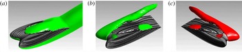
(a) Isosurfaces of spanwise vorticity in the reverse flow region and below the foil at
 ${\it\alpha}=5^{\circ }$
, (b,c) isosurfaces of streamwise vorticity in green (lighter) and red (darker) depicting opposite signs of vorticity values.

The deformation and separation of the forward and reversed flow boundary-layer vortex sheets are shown in figure 26(a–c) for the numerical data. Figure 26(a) illustrates the canopy-shaped vortex sheet that forms over the separation zone. Figures 26(b) and 26(c) depict the formation of streamwise vorticity on the surface of the tubercled foil at
 ${\it\alpha}=5^{\circ }$
, with the two signs of vorticity shown from different viewing angles. The deformation of the individual vortex lines near the surface agrees with the isosurface contours shown in this figure.
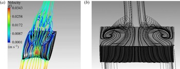
Three-dimensional streamlines at
 ${\it\alpha}=5^{\circ }$
: (a) formation of streamwise vortices and their trajectory downstream, (b) end view of streamwise vortex formation.

A plot of the three-dimensional streamlines is shown in figure 27(a). The origins of the streamwise vortices from the separation zone can be seen in this image. The reverse flow in the separation region is clearly evident. Figure 27(b) shows the end view of the streamwise vortex formation, emphasising the lift-off of the vortices from the surface of the foil.
Owl face of the first kind, after Perry & Hornung (Reference Perry and Hornung1984).

The topology shown in figure 28 resembles an ‘owl face of the first kind’, first defined by Perry & Hornung (Reference Perry and Hornung1984). The central vertical plane of the owl-face pattern corresponds to the tubercle trough in the present study. It can be seen that the primary vortices create upwash along the vertical plane, which confirms that the sense of rotation of the streamwise vortices is consistent with the current results. The structure is similar to that of stall cells on wings (Perry & Hornung Reference Perry and Hornung1984; Manolesos & Voutsinas Reference Manolesos and Voutsinas2014), which are classified as an owl face of the second kind (Perry & Hornung Reference Perry and Hornung1984), although the present structure is somewhat less complex.
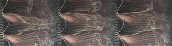
Flow visualisation for the
 $A8{\it\lambda}30$
tubercle configuration at an angle of attack
 ${\it\alpha}=10^{\circ }$
and
 $Re=4370$
. The patterns are frames from a video sequence which are spaced by 3 s. The images show the development of streamwise vortices behind the tubercle peaks, and it is shown that asymmetry develops over time. Flow is from left to right.

Figure 29 presents hydrogen bubble visualisation of the flow above the tubercled foil, showing clearly the rollup of vortices in a trough for the
 $A8{\it\lambda}30$
tubercle case. The appearance of the streaklines and the variations between the images demonstrate that the flow pattern varies with time. Asymmetry in the flow can be seen to increase with time in this image sequence; however, in later image frames (not shown here) the vortices appear to be symmetrical again. Therefore, the mean pattern consists of two counter-rotating vortices between the tubercle peaks, in agreement with the observations and interpretations made elsewhere in this paper. On the other hand, there is a certain degree of time dependence in the flow pattern, as has been alluded to previously, and this will be discussed further in § 8.
8. Time dependence of flow patterns
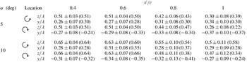
The vorticity and circulation results presented in §§ 3 and 4 were derived from velocity-vector fields which represented the average of 2085 image pairs. For a laser pulse rate of 10 Hz, the total acquisition time considered was approximately 209 s. The reason for averaging such a large number of samples was to reduce the uncertainty associated with imaging in a cross-flow plane. Based on a comparison between the time-dependent and averaged results, it was found that the averaged flow field data reflect the general flow behaviour. Quantification of the degree of unsteadiness was achieved through use of a peak detection algorithm that located the position of peak vorticity for each primary vortex in each instantaneous image. It was found that the mean position of these peaks corresponds well to the position of peak vorticity when the velocity fields are temporally averaged. The standard deviation is within reasonable limits and the movement of the vortices is best described as a fluctuation about the mean, as will be shown in § 8.1. Results are presented in table 3, and the units are consistent with other figures in this paper, whereby the
 $y$
- and
 $z$
-coordinates have been normalised by the tubercle wavelength.
Mean position and standard deviation of peak vorticity. The position of peak vorticity for temporally averaged experimental data is given in parentheses. All values are normalised by the tubercle wavelength of 30 mm.

Despite the general agreement between the mean and instantaneous results, some aspects of the flow patterns are influenced by unsteady effects, and these will be explored in this section.
8.1. Asymmetry
The temporal evolution of vorticity was investigated for the
 ${\it\alpha}=10^{\circ },x^{\prime }/c=1$
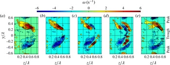
case to shed light on the unsteady effects that were discussed in § 3. The vorticity results of five sequential ensemble averages carried out over a period of 0.5 s each (five image pairs) are shown in figure 30(a–e). The sequence shown is representative of a common but intermittent cycle in the
 $x^{\prime }/c=0.8$
and
 $x^{\prime }/c=1$
cross-sectional planes at
 ${\it\alpha}=10^{\circ }$
. By comparison, the
 ${\it\alpha}=5^{\circ }$
case is less unsteady and thus shows less variation in the vorticity patterns.
A series of images showing the temporal evolution of vorticity for
 ${\it\alpha}=10^{\circ },Re=2230$
, image plane
 $x^{\prime }/c=1$
. Each pattern is averaged over five image pairs (0.5 s). It should be noted that vorticity with values in the range
 $-1\leqslant {\it\omega}_{z}\leqslant 1$
has not been plotted.

Figure 30 shows that, in this representative cycle, the primary vortices grow and move away from the foil surface, forming a canopy of vorticity behind the tubercle trough where the vortices interact before they collapse back towards the surface. During the interaction phase (c,d) there is an apparent ‘splitting’ of each vortex by layers of vorticity of opposite sign. The splitting is most apparent in figure 30(d). The prevalence of this process explains the existence of double lobes in figure 6(e) and the increased diffusion and rapid annihilation of vorticity shown in figures 5 and 6. The opposite-sign vorticity that is present in the primary vortex regions at certain times is also manifested as an attenuation of the vorticity across the measurement plane in the 209 s ensemble average. This attenuation in vorticity gives rise to a corresponding reduction in the magnitude of the experimentally derived circulation with respect to the numerically derived circulation at
 ${\it\alpha}=10^{\circ }$
, as shown in figure 16. The attenuation effects could mask the decrease in circulation seen at
 $x^{\prime }/c=1$
,
 ${\it\alpha}=10^{\circ }$
in the numerical results. This image sequence highlights the difficulty in interpreting ensemble-average flow patterns of highly unsteady and complex cases such as this.
Mean and fluctuating components of velocity for
 ${\it\alpha}=5^{\circ }$
,
 $Re=2230$
, image plane
 $x^{\prime }/c=0.8$
. Velocity units are
 $\text{mm}~\text{s}^{-1}$
, the
 $v$
velocity is in the
 $y$
-direction and the
 $w$
velocity is in the
 $z$
-direction.

Mean and fluctuating components of velocity for
 ${\it\alpha}=10^{\circ }$
,
 $Re=2230$
, image plane
 $x^{\prime }/c=1$
. Velocity units are
 $\text{mm}~\text{s}^{-1}$
, the
 $v$
velocity is in the
 $y$
-direction and the
 $w$
velocity is in the
 $z$
-direction.

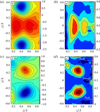
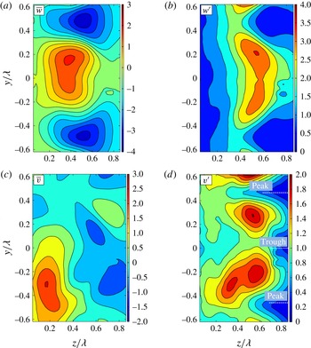
The unsteady nature of the flow for image planes close to the trailing edge of the foil is further explored through consideration of the mean and fluctuating velocity components in the
 $y$
and
 $z$
directions (
 $v$
and
 $w$
respectively), and these are shown in figures 31 and 32 for the
 ${\it\alpha}=5^{\circ }$
,
 $x^{\prime }/c=0.8$
and
 ${\it\alpha}=10^{\circ }$
,
 $x^{\prime }/c=1$
cases respectively. Comparison between figures 31 and 32 shows that the magnitudes of both the mean and fluctuating components of velocity in the
 ${\it\alpha}=10^{\circ }$
case are approximately three times those in the
 ${\it\alpha}=5^{\circ }$
case. In both cases it is also clear that the fluctuating velocity components are of similar magnitude to the corresponding mean components, confirming that the flow is highly unsteady for these cases. The following discussion assumes that fluctuation velocities are induced by temporal changes in the position of the vortex cores or the strengths of the vortices themselves.
The mean wall-normal component of velocity (
 $w$
-direction) is seen in both cases to be largest in the regions between the counter-rotating primary vortices, as expected. The shape and location of the peak
 $w$
-fluctuation on the right side of the trough is consistent with both a wall-normal and/or spanwise oscillation in the position of the primary vortex cores.
The mean spanwise component of velocity (
 $v$
-direction) is seen in the
 ${\it\alpha}=5^{\circ }$
case to be largest in regions to the right of the counter-rotating primary vortices, with a second peak left and outboard of each core adjacent to the foil surface. The
 $v$
-fluctuation peaks are located close to the
 $v$
-mean peaks, suggesting that the fluctuations are brought about by a relatively small wall-normal and/or spanwise oscillation in the position of the primary vortex cores. However, in the
 ${\it\alpha}=10^{\circ }$
case, the mean pattern in the
 $v$
-direction is highly asymmetric and less clearly defined, with the largest magnitude near the foil surface, to the left of one of the primary vortices. The peak fluctuations in this case are also asymmetric and they occur in regions of generally lower
 $v$
-mean values, suggesting that the flow is relatively more unsteady than in the
 ${\it\alpha}=5^{\circ }$
case.
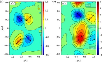
The fluctuating components are multiplied together at each grid position and ensemble averaged for (a)
 ${\it\alpha}=5^{\circ }$
, image plane
 $x^{\prime }/c=0.8$
and (b)
 ${\it\alpha}=10^{\circ }$
, image plane
 $x^{\prime }/c=1$
. For both cases,
 $Re=2230$
, velocity units are
 $\text{mm}~\text{s}^{-1}$
, the
 $v$
velocity is in the
 $y$
-direction and the
 $w$
velocity is in the
 $z$
-direction. Arrows indicate the overall fluctuation direction.

Finally, consideration of figures 32(b) and 32(d) together with the quasi-instantaneous vorticity fields of figure 30 shows that the velocity fluctuations support the observations made regarding the growth and collapse of a canopy of vorticity behind the tubercle trough. Specifically, for the
 ${\it\alpha}=10^{\circ }$
,
 $x^{\prime }/c=1$
case, the
 $w$
-fluctuation is large and the
 $v$
-fluctuation is small at
 $(y/{\it\lambda},z/{\it\lambda})=(0,0.6)$
, where the motion of the canopy is seen to be primarily in the wall-normal
 $(z)$
direction. Furthermore, figure 33(b) indicates that both the
 $v$
- and
 $w$
-fluctuations are large at or near
 $(y/{\it\lambda},z/{\it\lambda})=(\pm 0.25,0.5)$
and
 $(\pm 0.2,0.8)$
, consistent with the canopy of vorticity expanding in height and width and then collapsing again. A similar pattern can be observed in figure 33(a) at
 ${\it\alpha}=5^{\circ }$
,
 $x^{\prime }/c=0.8$
; however, the concurrent peaks in the
 $v$
- and
 $w$
-fluctuations occur closer to the foil surface for this case.
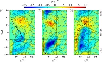
Sequence of vorticity plots on the image plane
 $x^{\prime }/c=0.8$
for
 ${\it\alpha}=10^{\circ },Re=2230$
, where transport of wall vorticity is shown with the black arrows. (a) Negative wall vorticity entrained by clockwise rotating primary vortex, (b) intermediate state and (c) positive wall vorticity entrained by anticlockwise rotating primary vortex.

Schematic showing wall vorticity close to the surface being entrained by the primary vortices at adjacent locations. Dashed arrows indicate transport of vorticity to adjacent troughs between tubercles.

8.2. Unsteady contribution to the streamwise increase in circulation
The dominant mechanism responsible for the streamwise increase in circulation observed in both the experimental and numerical results presented in § 5.1 is steady in nature and was discussed in § 7. On the other hand, an unsteady mechanism was also observed in the experimental results. To further examine this mechanism, vorticity was plotted for a series of images for the
 ${\it\alpha}=10^{\circ }$
,
 $x^{\prime }/c=0.8$
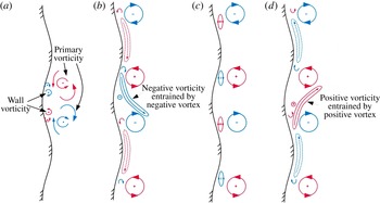
case. Each image is an average of 15 image pairs and represents 1.5 s in time. The three images shown in figure 34 illustrate that vorticity is transported from the region adjacent to the wall to the streamwise vortices. In figure 34(a) the negative wall vorticity is entrained by the clockwise rotating vortex. Figure 34(b) represents an intermediate state and in figure 34(c) the positive wall vorticity is entrained by the anticlockwise rotating vortex.
Therefore, a proposed unsteady mechanism for the increase in circulation with streamwise location is shown in figure 35, where the primary and wall vortices are indicated in figure 35(a). It can be seen in figure 35(b) that the negative wall vorticity near the surface is entrained by the negative primary vortex, which describes one extreme pattern of the flow. The opposite extreme pattern is shown in figure 35(d), and the pattern shown in figure 35(c) represents the intermediate state. This mechanism may also involve vorticity transported to vortices formed behind adjacent tubercles, as indicated by the black arrow at the bottom of figure 34(b) and in figure 35 by the dashed arrows which show flow movement from adjacent vortex pairs. The unsteady mechanism is likely to be of secondary importance to the steady mechanism discussed in § 7 since both the experimental and numerical results indicate a streamwise increase in circulation.
9. Discussion and conclusions
The combined experimental and numerical studies have identified the salient features of the flow structure produced by a NACA 0021 foil with tubercles at a Reynolds number of 2230. The presence of the tubercles leads to an increased flow velocity along the trough, and a larger adverse pressure gradient. This in turn causes boundary-layer separation to occur in the trough at a low angle of attack. These findings are consistent with previous research, where the larger adverse pressure gradient in the trough region was attributed to the relatively short chord length at this spanwise location (van Nierop et al. Reference van Nierop, Alben and Brenner2008). Hence, the same pressure difference needs to be overcome over a shorter distance behind a tubercle trough relative to a tubercle peak (van Nierop et al. Reference van Nierop, Alben and Brenner2008). Previous studies have also identified the presence of a spanwise pressure gradient (Skillen et al. Reference Skillen, Revell, Pinelli, Piomelli and Favier2014), and the results presented here indicate that this is most significant in the region of the leading edge, where the minimum suction peak occurs. It has been shown that the spanwise pressure gradients, set up by the tubercles, interact with the vorticity distribution, leading to a complex flow pattern. The numerical simulation of the flow is in strong agreement with the experimental observations and allows close examination of the flow structure. The resulting three-dimensional pattern bears a strong similarity to the owl face of the first kind, first described by Perry & Hornung (Reference Perry and Hornung1984).
Analysis of the flow field data obtained from both PIV experiments and CFD modelling reveals regions of vorticity of alternate sign in the troughs between tubercles for all spanwise planes investigated. The presence of these streamwise vortices has been shown in previous work (Custodio Reference Custodio2007; Pedro & Kobayashi Reference Pedro and Kobayashi2008; Stanway Reference Stanway2008; Skillen et al. Reference Skillen, Revell, Pinelli, Piomelli and Favier2014); however, the spanwise location of vorticity was not clear in these results and the vorticity was not quantified as it has been in this study. The current work also shows for the first time that the counter-rotating streamwise vortices lift away from the surface at a certain chordwise location, corresponding to the large foci in the surface streamline (shear stress) pattern, the locations of which are governed by the angle of attack of the foil. At this point, the flow field becomes highly unsteady and the distribution of vorticity in the region of the primary vortices varies with time, a feature that has not been previously identified.
Considering the averaged experimental results, the magnitude of the peak primary vorticity has been shown to decrease in the streamwise direction, while the region of vorticity expands in area. This effect can be attributed to axial compression of the streamwise vortices caused by the adverse pressure gradient on the suction surface of the foil, vortex tilting and viscous diffusion of vorticity. The results also indicate that the circulation of the primary pair of streamwise vortices increases with streamwise distance, achieving a maximum value at the trailing edge. The increase in circulation occurs due to continued influx of boundary-layer vorticity which occurs along the sides of the shear-layer canopy. An increasing vortex circulation in the streamwise direction has also been observed for delta wings (Visser & Nelson Reference Visser and Nelson1993; Johari & Moreira Reference Johari and Moreira1998), but this has not been shown for a tubercled wing prior to this study. This supports the theory that tubercles can be modelled as delta wings with a rounded leading edge (Weber et al. Reference Weber, Howle, Murray and Miklosovic2011).
The numerical study provides novel insights into the flow structure and evolution of vorticity in the flow cases under investigation. The computed sectional velocity and vorticity fields show a strong correspondence to the experimental results. An analysis of the surface vortex lines reveals a number of regions where local turning of the vorticity leads to the formation of streamwise vorticity in the boundary layer, beginning on the sides of the tubercles and occurring at various locations all the way to the trailing edge. The results also demonstrate a source of reverse-sign secondary vorticity beneath the primary vortices downstream of the foci, which was shown to occur near the wall in both the experimental and numerical results. These observations are corroborated by the isosurfaces of streamwise and spanwise vorticity presented in figure 26. The turning of the boundary-layer vorticity from a spanwise-dominant orientation towards the streamwise direction suggests the development of Prandtl’s secondary flow of the first type. This is a quasi-inviscid mechanism which is activated by the presence of skewness in the flow, arising from spanwise pressure gradients. This mechanism has been observed to operate for a foil with tubercles in the transitional flow regime (Rostamzadeh et al. Reference Rostamzadeh, Hansen, Kelso and Dally2014) and is also observed to be at play in the laminar flow regime investigated in this study. The local turning of vorticity was also observed by Favier et al. (Reference Favier, Pinelli and Piomelli2012); however, these researchers referred to vorticity that was initially normal to the surface, rather than being aligned in the spanwise direction. The generation of the vorticity is not attributed to a Kelvin Helmholtz instability which was referred to by Favier et al. (Reference Favier, Pinelli and Piomelli2012).
In general, there is strong correspondence between the experimental and numerically derived magnitudes and trends of the peak vorticity and circulation of the primary vortices. The main differences lie towards the trailing edge of the foil in the
 ${\it\alpha}=10^{\circ }$
case. In the numerical results, the slight decrease in the circulation between
 $x^{\prime }/c=0.8$
and 1 is attributed to a source of negative vorticity in the reverse flow, as shown in figure 26(b,c). In the experimental results, no sudden drop is observed, but the overall magnitude of primary vortex circulation is generally lower than in the corresponding CFD results. While some of these differences may be due to inadequacies in the transitional SST closure model used in the numerical study, the effects of unsteadiness are also likely to be a significant cause. In particular, the time-variant nature of the flow pattern demonstrated in § 8 indicates the high degree of unsteadiness near the trailing edge for both
 ${\it\alpha}=5^{\circ }$
and
 ${\it\alpha}=10^{\circ }$
. Unsteadiness of this magnitude, greater in the
 ${\it\alpha}=10^{\circ }$
case, will result in axial and lateral oscillation of the flow pattern, leading to a higher rate of generation, diffusion and annihilation of the vortices in the flow, consistent with the structure shown in figure 30. From a measurement perspective, the unsteadiness will lead to attenuation and spreading of the time-averaged vorticity across the measurement plane as well as in the streamwise direction, obscuring the instantaneous flow structure. In fact, due to the strong influence of unsteadiness in this flow, it is likely that small errors in the computed flow structure due to the choice of closure model, such as the axial location of the flow separation, will not affect the validity of the CFD results as an interpretive tool.
The aerodynamic performance of a NACA 0021 foil with
 $A8{\it\lambda}30$
tubercles has been shown to be slightly better in comparison to an unmodified foil under the conditions of this study. Improved performance has also been observed in previous studies under different flow conditions (Watts & Fish Reference Watts and Fish2001; Miklosovic et al.
Reference Miklosovic, Murray, Howle and Fish2004). Integration of the pressure distributions at various chordwise locations has revealed that the largest amount of lift is generated at a cross-section corresponding to a tubercle peak. This is consistent with the observation that flow separation occurs further aft at this location. A delayed separation at the peak cross-section has also been observed in previous studies (Johari et al.
Reference Johari, Henoch, Custodio and Levshin2007; van Nierop et al.
Reference van Nierop, Alben and Brenner2008; Hansen et al.
Reference Hansen, Kelso and Dally2011).
In spite of the strong correspondence between the experimentally and numerically determined flow features and trends, there are still a number of unresolved features, such as the regions of vorticity marked with an asterisk in figures 5 and 6. Further investigation into the time-dependent characteristics of the flow field surrounding a foil with leading edge tubercles is suggested for future work. In particular, it would be useful to study the three-dimensional evolution of the streamwise vortices in the unsteady flow to gain more insight into the formation and annihilation processes which were touched upon briefly in this paper.
Appendix A. Uncertainty analysis
The most significant bias uncertainty with respect to particle displacement is attributed to the perspective error. This was estimated to be in the range of 0–12%, depending on the size and position of the vortices. A greater distance between the particle of interest and the centreline of the image plane would lead to a larger uncertainty in particle displacement.
The sources of random uncertainty that were deemed to have the most significant impact on the results are related to the following parameters: laser jitter,
 ${\it\delta}_{t}$
; particle image diameter,
 ${\it\delta}_{e}$
; uncertainty in particle displacement,
 ${\it\delta}_{{\rm\Delta}D}$
; seeding density,
 ${\it\delta}_{N}$
; magnification,
 ${\it\delta}_{m}$
; and the displacement gradient,
 ${\it\delta}_{g}$
. Where relevant, a seeding density of approximately 20 particles per interrogation window was assumed in the following analysis based on visual inspection of the raw data. A particle displacement of 0.9 px is assumed, as this was a typical amount by which a particle within the vortex core was displaced between laser pulses.
The camera jitter was determined from manufacturer’s specifications, where
 ${\it\delta}_{t}=250~\text{ns}$
. The uncertainty related to the particle image diameter was found in Raffel et al. (Reference Raffel, Willert and Kompenhans2007, figure 5.32a), where
 ${\it\delta}_{e}=0.03$
. The uncertainty in particle displacement was determined in Willert & Gharib (Reference Willert and Gharib1991, figure 6b), where
 ${\it\delta}_{{\rm\Delta}D}=0.04$
. The uncertainty related to seeding density is given in Raffel et al. (Reference Raffel, Willert and Kompenhans2007, figure 5.40), where
 ${\it\delta}_{N}=0.05$
. The uncertainty arising from the magnification scale used was estimated by visual inspection of the target image, giving
 ${\it\delta}_{m}=0.002$
. The displacement gradient was determined in the region of the vortex by plotting the particle displacement along axes that intersect the vortex core. The slope of these plots corresponds to the displacement gradient, where the maximum is approximately 0.015 for the
 ${\it\alpha}=10$
,
 $x^{\prime }/c=1$
case. The value of the uncertainty related to the displacement gradient was then determined in Raffel et al. (Reference Raffel, Willert and Kompenhans2007, figure 5.42), where
 ${\it\delta}_{g}=0.04$
.
The relative uncertainties related to laser jitter and magnification were normalised by the time delay between image pairs,
 ${\rm\Delta}T$
, and the grid width,
 $w_{g}$
, respectively. All other relative uncertainties were normalised by the value of a typical displacement in the region of the vortex core of 0.9 px. The overall uncertainty,
 ${\it\varepsilon}_{u}$
, for a given image pair was determined by combining the relative uncertainties as
 $$\begin{eqnarray}{\it\varepsilon}_{u}=\sqrt{\left(\frac{{\it\delta}_{t}}{{\rm\Delta}T}\right)^{2}+\left(\frac{{\it\delta}_{e}}{{\rm\Delta}D}\right)^{2}+\left(\frac{{\it\delta}_{{\rm\Delta}D}}{{\rm\Delta}D}\right)^{2}+\left(\frac{{\it\delta}_{N}}{{\rm\Delta}D}\right)^{2}+\left(\frac{{\it\delta}_{m}}{w_{g}}\right)^{2}+\left(\frac{{\it\delta}_{g}}{{\rm\Delta}D}\right)^{2}}=0.08.\end{eqnarray}$$
The error propagation analysis of Fouras & Soria (Reference Fouras and Soria1998) with reference to Lau (Reference Lau2010) was applied to determine the maximum random and bias uncertainty in vorticity, which are 6 % and 1.4 % respectively for an instantaneous velocity-vector field. Thus, the maximum total uncertainty in vorticity is approximately 6.4 %. The random uncertainty in vorticity for the averaged data is determined by finding the overall uncertainty in particle displacement for an average of 2085 image pairs:
 ${\it\varepsilon}_{u(avg)}=0.06/\sqrt{2085}=0.0013$
. The overall uncertainty in vorticity for the averaged data is thus dominated by the bias uncertainty of 1.4 %.
Details of the method and the associated uncertainty analysis for circulation are given in Hassan et al. (Reference Hassan, Lau and Kelso2007, figures 2 and 3). The maximum random and bias uncertainties are 3 % and 15 % respectively. Hence, the total uncertainty in circulation for an instantaneous velocity-vector field is 15.3 %. Once again, the uncertainty for the average data is substantially lower and should be less than 1 %.