

When the Republican Governor of Maryland, Larry Hogan, took office in 2015, he withheld $68 million in funding for high-cost school systems. This decision directly impacted Prince George’s and Montgomery counties, which would have received $20 million and $17 million in extra money each. Interestingly, these counties had overwhelmingly supported the Democratic opponent to Hogan in the election (Hicks Reference Hicks2015). Was the decision to withhold funds politically motivated or just a cost-saving measure? While state funding for education programs has been debated vigorously from ballot boxes to court rooms, the debates often center on economic arguments. Many states rely on a funding formula to distribute education funds to local school districts with the idea that this distribution is at least partially determined by a local district’s property tax base. This mathematical formula is often touted as a way to fairly distribute funds, but the formula often lacks transparency and can be quite complex. Do politicians manipulate the formula so that it rewards their core constituents more?
Political science research offers evidence that politicians distribute benefits to loyal or core voters in hopes of maximizing electoral benefits. Much of this evidence has focused on federal distributions to congressional districts or, in a few cases, state distributions to counties. While counties do define geographically similar areas, they are less likely to define homogeneous populations in terms of voting preferences. An urban area is likely to be more politically similar to other urban areas in different counties than it is to the rural area within the same county. Funding for public education provides an opportunity to test how strategic state elected officials are in distributing benefits to like voters because it defines a more homogeneous constituency. In addition, public education is the largest expenditure of local and state governments (Bernstein Reference Bernstein2014). With large shares of money at the state level to transfer to local governments and the ability to target core voters, it would seem likely that politicians would take advantage of this. This article tests whether education funding is influenced by the core voter model, with districts that support the state party in power receiving more benefits.
This article uses a novel data set to test whether the consistency between state party control and the partisanship of a local school district influences state transfers to that district. I collected data at the precinct level within each state and, using mapping software, spatially joined precinct boundaries to school district boundaries. Once this relationship was established, I was then able to aggregate precinct-level information up to school districts to understand the partisan voting patterns within each school district for elections from 2000 to 2010. There data were supplemented with voting data at the county level for presidential elections from 1992 to 2012 as a comparison. By combining these data with financial and demographic information of a school district, I was able to leverage changes in partisanship over time at the state level to test how it influences the distribution of funds in subsequent years.
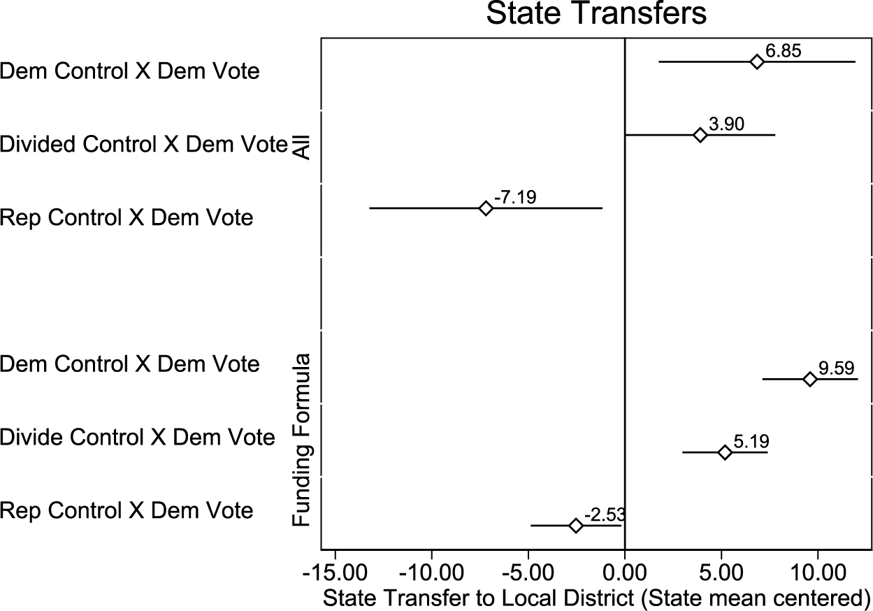
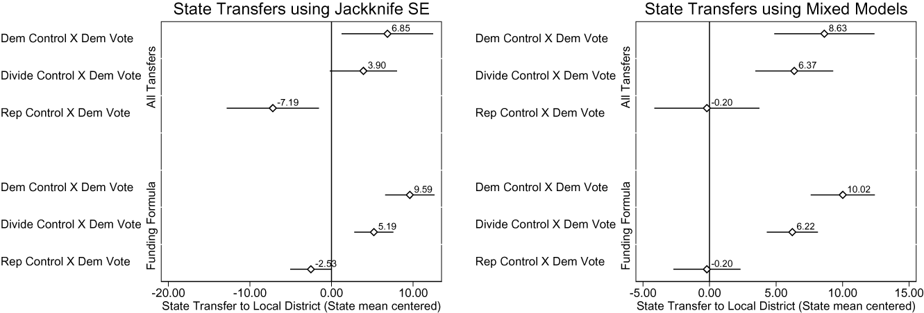
I find evidence that funding formulas are susceptible to political influence and that parties are able to influence the geographic distribution of education funds to core voters. I find a strong relationship when state party control and local partisan support align, focusing exclusively on school districts. If there was no partisan influence in funding formulas, then we would expect that the percent voting for a Democratic candidate would be unrelated to the amount a district receives. However, a 1 percentage point increase in voting for the Democratic candidates in an election when Democrats have control at the state level is associated with a $9.59 per student increase to funding from the state formula, above the state mean. If Republicans have control at the state level, then a 1 percentage point increase in voting for the Democratic candidates is associated with a $2.53 decrease in state transfers, relative to the state mean.
Distributing Public Goods
Funding for public education in the United States is a complicated process that involves all levels of government. In the 2011–2012 school year, states provided approximately 42% of public school revenues, local districts provided 46%, and the federal government provided 12%. However, there is considerable variation from state to state. For example, the state of Vermont contributed more than 85% of the revenue, whereas Illinois contributed less than 30% (Odden and Picus Reference Odden and Picus2014). The ways in which states distribute their money to local school districts can vary as well. Over the years, courts and state legislatures have sought to equalize school funding within a state through these various methods of transferring money. Intergovernmental transfers can occur through grants or through a funding formula. Grants, whether unrestricted, categorical, or matching, are sums of money transferred to a district. State funding formulas are methods for transferring money back to local government and often done through a flat-grant, foundation program, or guaranteed tax base (GTB) program (Odden and Picus Reference Odden and Picus2014).Footnote 1 Some states use a combination of the types. Hawaii, which only has one school district, fully funds the school district.
Much of the research in understanding funding formulas has focused on the economic components of the formulas and whether or not they achieve equalization.Footnote 2 The assumption frequently is that the goal of the process is apolitical and that the process is trying to redistribute money based on need determined by the local tax base. That is, the focus is on the link between local property taxes and per pupil revenue and how that leads to fiscal inequalities (i.e., Alexander and Salmon Reference Alexander and Salmon1995; Guthrie et al. Reference Guthrie, Springer, Anthony Rolle and Houck2007; Odden and Picus Reference Odden and Picus2014). The inequality is created by uneven tax bases, and therefore creates uneven spending per pupil.
But there is a significant amount of research that shows that parties distribute goods to optimize electoral outcomes. Elected officials respond more to voters than to nonvoters (Griffin and Newman Reference Griffin and Newman2005), and voters enjoy better policy representation and are rewarded more than nonvoters (Griffin and Newman Reference Griffin and Newman2012). In designing redistribution programs, elected officials have the opportunity to reward key legislative districts and ignore districts that they believe will not be beneficial electorally (Dixit and Londregan Reference Dixit and Londregan1996). Scholars have debated the strategy that elected officials use to target voters. Elected officials could follow the core voter model (or loyal voter), in which money is allocated to areas that contain core voters (Cox Reference Cox, Shapiro, Stokes, Wood and Kirshner2010; Cox and McCubbins Reference Cox and McCubbins1986), or a swing voter model, in which money is allocated to pivotal electoral areas (Lindbeck and Weibull Reference Lindbeck and Weibull1987). While both of these models are derived through game theoretic models, empirical work has found support for these models as well.Footnote 3
When deciding which model is appropriate, the goal of the party must be understood. Are the parties trying to persuade voters, mobilize voters, or coordinate voting efforts? If the goal is only to persuade voters to choose between two parties and turnout is set, then the research is mixed in what parties are trying to achieve when they distribute public goods. If, however, parties are also trying to mobilize voters to turnout or affect the number and character of alternatives from which voters choose, then there is much more support for the core voter model (Cox Reference Cox, Shapiro, Stokes, Wood and Kirshner2010). There is ample evidence of this at the federal level. An increase in federal spending benefits is associated with an increase in support in the popular vote for the incumbent in House elections (Levitt and Snyder Reference Levitt and Snyder1997). In an analysis of distribution of Federal Emergency Management Agency (FEMA) aid after Hurricane Katrina, Chen (Reference Chen2013) finds that the aid had an interesting impact on turnout. Not only did turnout increase for the incumbent party but it also decreased for the opposition party in response to aid given in the aftermath of the disaster. Incumbents who are vulnerable electorally might be more likely to seek out new money to bring to a congressional district to shore up votes (Stein and Bickers Reference Stein and Bickers1994). Legislatures are strategic in getting resources to those most likely to support and vote for them.
Much of this research has focused on the federal level, with a few exceptions of state transfers to counties (Ansolabehere, Gerber, and Snyder Reference Ansolabehere, Gerber and Snyder2002; Ansolabehere and Snyder Reference Ansolabehere and Snyder2006). Can and are parties at the state level able to be more direct in their targeting of benefits? While counties do define geographically similar areas, they often do not define homogeneous populations. School districts, on the contrary, often capture much more homogeneous populations. Not only do they often represent much smaller regions than counties, the ways in which school district boundaries were formed created more homogeneous groups. There are more than 12,000 school districts throughout the United States. This might allow state legislatures to target urban or rural voters more easily. Research has highlighted that school district boundaries, as well as other types of political boundaries, can serve in ways to keep residents more homogeneous and exclude certain races or economic classes (Bischoff Reference Bischoff2008; Danielson Reference Danielson1976; Weiher Reference Weiher1991). Therefore, school districts represent areas that politicians should be able to more strategically distribute benefits than counties or even congressional districts.
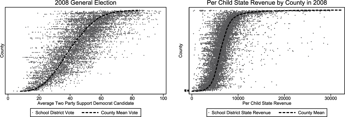
Figure 1 illustrates the variation in both voting and state transfers to school districts that occur within counties in the United States. Each row represents the vote in a county and school districts within that county. In the figure on the left, the gray dots represent the two-party vote for that school district, and the dark, dashed line represents the county mean. While there is obviously correlation between the average county vote and a school district’s vote within each county, there is clearly significant variation within each county in the two-party vote for a Democratic candidate. For example, in some counties where the county vote went well over 60% in favor of Democrats, some school districts within those counties voted less than 20% in favor of the Democratic candidate. The figure on the right is the same setup but with per child state transfers to a school district. Again, there is correlation between county means and what was transferred within the county to school districts but with significant variation within each county.
County mean compared to school district.
Note. The figures illustrate the variation between school districts within a county. Each row represents a county, and each dot is a school district within that county. The figure on the left shows variation in voting within a county, and the figure on the right shows variation in state transfers to a school district within a county.

Furthermore, it is important to note that Republican and Democratic parties have different platforms on education, and therefore might pursue different strategies in funding education. Following Cox and McCubbins (Reference Cox and McCubbins1986), the strategies that legislatures will pursue are ones that will benefit their constituents the most. Democrats are likely to favor strategies that target areas with higher need, while Republicans might favor strategies that focus on efficiency of spending or increased school choice. The Democratic party has argued for higher levels of funding, while Republicans have argued that additional funding will not solve problems faced in education (Meier and Rutherford Reference Meier and Rutherford2016). In analysis of states, Hill and Jones (Reference Hill and Jones2017) find that Republican and Democratic governors allocate spending differently, with Democratic governors allocating higher shares of state transfers to minority students.Footnote 4
In addition, teacher unions provide an avenue in which to alert state-level politicians to school district voting behavior. Moe (Reference Moe2005) has found that teacher unions mobilize both their members and other voters in elections. Political activity by teacher unions has been shown to reduce the likelihood of certain reform-style policies at the state level, such as school choice (Hartney and Flavin Reference Hartney and Flavin2011). Teacher unions are major contributors to state legislature races (Lott and Kenny Reference Lott and Kenny2013), and teachers themselves vote at higher rates than average citizens (Wolfinger and Rosenstone Reference Wolfinger and Rosenstone1980). Because of this relationship, state legislatures are likely paying attention to party support at the district level. Furthermore, the Democratic Party has a much stronger relationship with teacher unions. The two largest teacher unions give 95% of their campaign and soft money contributions to Democrats (DeBray-Pelot and McGuinn Reference DeBray-Pelot and McGuinn2009).
But how much influence do state legislatures have over funding formulas? Because of the unequal nature of school funding, many funding formulas have been challenged in court. In the landmark case, Serrano v. Priest (1971) found California’s financing of schools to be unconstitutional (Berkman and Plutzer, Reference Berkman and Plutzer2005). They held that education was a fundamental state right, greatly changing how education spending was determined in California and set off a wave of court challenges to funding formulas (Berkman and Plutzer Reference Berkman and Plutzer2005). As of 2017, 45 states have had their finance system challenged, with about half the states having had their funding systems completely or partially overturned by state’s courts (Rebell Reference Rebell2017). The second wave of school finance reform began in 1989 with a ruling by the Kentucky Supreme Court requiring that each child in the state must have an equal opportunity to have an adequate education (Lafortune, Rothstein, and Schanzenbach Reference Lafortune, Rothstein and Schanzenbach2018). Lafortune, Rothstein, and Schanzenbach (Reference Lafortune, Rothstein and Schanzenbach2018) identified 64 school finance reform events between 1900 and 2011 in 26 different states. The court systems do generally have a significant impact on the distribution of educational resources. However, inequality is often not reduced (Reed Reference Reed2003). This suggests that there is opportunity to influence the distribution of money through changes in the funding formula in ways that could support a core voter model. While changes to funding formulas can occur incrementally, these rulings have led to many opportunities for the party in control at the state level to overhaul an existing formula.
School districts themselves may be strategic in providing forecasts of local revenue to “state policymakers who regularly tinker with state funding formulas” in hopes of showing more need to get more from the state (Lavertu and St. Clair Reference Lavertu and St. Clair2018, 60). It is also possible that the strategies that each party pursues to fix funding issues are likely to be the most advantageous to their core supporters. Democrats might be more likely to pursue strategies that help school districts in high-poverty, high-minority areas. Republicans might be less inclined to increase spending, instead focusing on being more efficient. Therefore, these higher need districts would not get any additional money.
Transfers can happen outside the formulas as well. For example, New York has bullet aid funding, that is, money that is distributed outside the funding formulas to school districts at the end of each fiscal year. In 2015, $15 million were distributed to schools through this type of funding (Flanagan and Klein Reference Flanagan and Klein2016). The spokesman for the New York Assembly Speaker Carl Heastie, Michael Whyland, said, “The school aid formula can’t account for every situation among the nearly 700 school districts statewide, so this is funding to schools that need it” (Harris Reference Harris2015). However, there is little transparency in how or why this money is distributed to certain districts. In addition, block grants are often given for many different areas such as special education, lunch programs, bilingual education, or transportation to make up for gaps in the funding formula. Partisanship can influence which types of programs to support. Different programs can be distributed differently, such as need-based or equality in distribution.
With opportunity to influence the distribution of education funds to different geographic locations and the ability to target populations of similar voters in school districts, state transfers for education are likely to follow the core voter model. School districts provide an excellent way to test the core voter model and see how strategic state parties are in distributing benefits to a more granular population. I hypothesize that districts that vote for the party in power at the state level receive more benefits, in terms of state transfers per child, than districts that support the opposing party. I do not focus on differences in specific funding formulas because many states take a combination approach when determining how to allocate money. However, I do run separate models on all transfers and funding formula transfers separately to see whether funding formula itself is more susceptible to partisan influences. In addition, I run additional models to see whether parties are targeting areas of likely supporters or areas of greater need, but not necessarily voters themselves.
Data and Method
Using precinct-level election data, school budget data, student demographic data, and community demographic data, I created a data set from 2000 to 2010. This analysis consists of 33 states that I was able to obtain precinct-level information. I supplement this data set using county-level voting data from 1992 to 2012 that include all states. Table 1 summarizes the data used for models that use precinct-level voting data. Table B.2 in Supplemental Appendix summarizes the data used for models that use county-level voting data. I first discuss the data used to capture partisanship at the state and local level. Then, I discuss demographic and financial data.
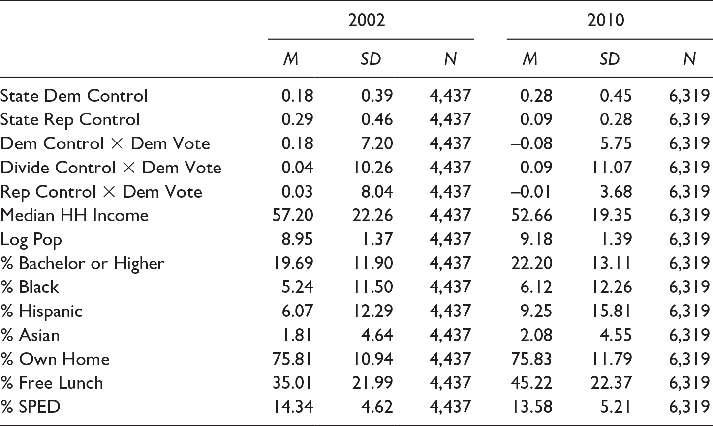
Summary Statistics.

Note. This table presents district-level data for select years of the data set. The two-party Democratic vote is relative to the state mean. HH = household; % SPED = percentage enrolled in special education.
Election Data
To understand the congruence between state and local school district partisanship, information about both state party control and local support for parties is needed. For state-level information, I use data on state party control from Klarner (Reference Klarner2013). These are yearly data that identify which party has control of the legislative and executive branch within each state and whether the party in control has a veto-proof majority. I follow the definitions of state party control used by Ansolabehere and Snyder (Reference Ansolabehere and Snyder2006) in their analysis of state transfers to counties. Therefore, I define a state as being under Democratic control if the Democrats have a majority in both legislative chambers and the governor is a Democrat or if the Democrats have a veto-proof majority in both legislative chambers. The same definition is applied for Republican control. Divided control occurs when neither major party has control. Table B.1 in Supplemental Appendix shows the number of years that the state has had Democratic, Republican, or divided party control. It also indicates whether that state is included in the analysis.
State-level control is determined based on the budget cycle of that state. States have either an annual or a biannual budget cycle. Depending on which process a state has, I look at either the previous year or the previous two years to determine party control. If it is an annual budget cycle, a period of Democratic Control is defined if in the previous year Democrats controlled the state legislature. Republican control would require Republicans to be in control, while Divided control would be defined if neither party had control in the previous year. In states that have biannual budget cycles, I look at the previous two years to define control.
As a robustness check, I look at two additional time frames of party control. I first use an eight-year window of control. This is the same definition used by Ansolabehere and Snyder (Reference Ansolabehere and Snyder2006). They select this time frame because policies often take time to implement and budget changes are often slow-moving. A period of Democratic Control in a state is defined if Democrats maintained control for at least four of those years and Republicans had control for three or fewer years (or it could also be under divided control for four or fewer years). Republican control during this eight-year window would require four or more years of Republican control. Therefore, when I am predicting the intergovernmental transfers for the 1993 school year, I focus on the party in control during the years 1985–1992. If Democrats maintain control for at least four of those years, it is coded as under Democratic Control. The variables are defined by Democratic Control, Republican Control, and Divided Control. Finally, I create a time frame of four years of party control. This allows me to split the difference between the shorter time frame of a budget cycle and the longer time frame of the eight-year window.
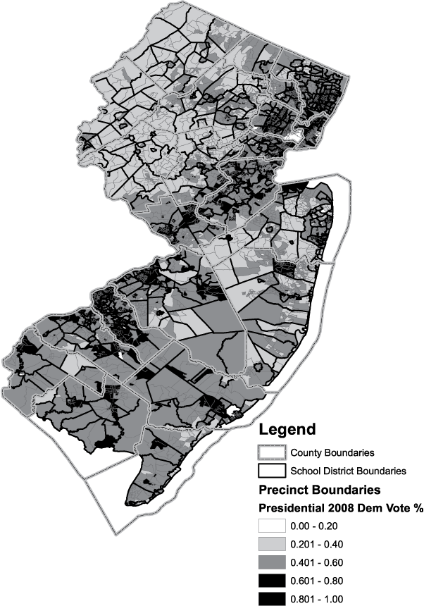
To determine the congruence with local voters, I first focus on precinct-level data. Because counties group a large share of voters together and can have multiple school districts, I use precinct-level data to obtain a more granular picture of partisan turnout within each school district. Precincts or voting districts are smaller divisions within a county and can be aggregated to show the vote within a school district. Figure 2 illustrates just how different a county two-party vote and the school district votes within the county can be by using New Jersey as an example. County boundaries are represented by dashed lines, while school district boundaries are in dark black. The average vote for the two-party 2008 Democratic presidential election for each precinct is color-coded based on the degree of support. For example, within Camden, there are 35 different school districts. The average Democratic presidential vote in the 2008 election in Camden was 67.5%, but there was wide variation at the precinct level. On the low end, the vote in Waterford Township School District was 53.7%. On the opposite end, the vote in Lawnside Borough School District was 97.4%. By using precinct-level data, I have a more accurate view of support for a party within a school district.
New Jersey by county, school district, and precinct boundaries.
Note. The figure illustrates the variation in voting that occurs within a county.

I run a robustness check with county-level election data to see what difference the more granular data make. Presidential election data are collected at the county level for the following years: 1988, 1992, 1996, 2000, 2004, 2008, and 2012. This information was compiled from CQ Press (2016) by state and election year. I use these data to identify the average two-party vote received by the Democratic candidate for president for the previous two elections within a county. Therefore, when I am predicting the intergovernmental transfers for the 1993 school year, I would use the 1988 and 1992 election results. This variable is called Dem Vote C. This county-level information serves as a proxy for district partisanship.Precinct data are not inherently connected to school district boundaries. To make this connection, I used the mapping software ArcGIS to match precinct boundaries to school district boundaries.Footnote 5 Table B.1 in Supplemental Appendix provides the source used for precinct boundaries for each state. This resulted in 33 states that are included in this analysis.Footnote 6 School district boundaries were mapped using data from the National Center for Education Statistics (NCES 2013). For the majority of cases, a precinct was defined to be within a school district if it fell completely inside the school district boundaries. However, there are cases in which a precinct crossed school district lines. When this occurred, the votes for that precinct were counted in all school districts for which it fell inside. Please see Supplemental Appendix A for additional details about the mapping process.
Once the crosswalk between precincts and school districts was complete based on 2010 boundaries, I created crosswalks across different election years. Data collected by Ansolabehere, Palmer, and Lee (Reference Ansolabehere, Palmer and Lee2014) contain precinct-level voting data by state for elections between 2000 and 2012. This includes results for presidential, governor, U.S. House, and U.S. Senate elections. While some states use the same name or precinct code across elections, other states were less consistent in their naming conventions and coding. Through extensive cleaning, I was able to match most precincts over this time frame. Detailed code can be provided upon request that matches precincts across years.Footnote 7 Vote counts for each election type and year were then aggregated to the school district level. Most years have more than one election; therefore, I take the average Democratic vote across elections within a year. The average two-party vote for a Democratic candidate is rescaled so that it represents the deviation in state party support and local party support. Because there is variation from state to state in average Democratic support, this allows a more accurate comparison of divergence or congruence from state averages. As an example, if the state average two-party vote was 51% and the district vote was 55%, then the district supported the Democrats 4 percentage points more than the state average. This variable is called Dem Vote Precinct.
T to understand the impact of the party in power at the state level and its relation to the school district vote, I create an interaction between the two. Therefore, Dem Vote Precinct Footnote 8 is interacted with Dem Control, Republican Control, and Divided Control to create Dem Vote Precinct × Democrat Control, Dem Vote Precinct × Republican Control, and Dem Vote Precinct × Divided Control.Footnote 9 As Ansolabehere and Snyder (Reference Ansolabehere and Snyder2006) note, these variables measure the direction that the governing party skews funds. The expectation is that if Democrats are in control at the state level, then they would award more money to districts that support Democratic candidates. This interaction captures this relationship. Finally, I include a variable that indicates how close the vote was within the district. Close Vote 50-50 indicates how close the vote was between the two parties. A value of 0 would indicate that the Democrats and Republicans received the same percentage of the vote; a value of 15 would indicate that one party received 15 percentage points more than the other party.
School District Information
In addition to partisanship information, financial information for each district was collected. To measure the transfers from state to local governments, I use the Public Elementary–Secondary Education Finance Data provided by the U.S. Census Bureau from 1995 to 2011 (U.S. Census Bureau 1993–2011) This data set breaks apart revenue by local, state, and federal governments and provides what each district receives from each level of government.Footnote 10 In addition, state-level revenue is further refined by denoting the source. That is, the funding is detailed by whether it is a transfer from a general funding formula, a special education program, or a bilingual education program, as examples. All dollar amounts are in 2013 constant dollars.
This data set is the source for the main dependent variables: a per student measure of all state funds to a district and a per student measure of funds from a general formula assistance. Districts vary in size and states vary in their capacity to provide education funding. To understand how one district’s revenue from the state compares to another district within the same state, I transform each dependent variable so that it is in relation to the state mean. That is, the dependent variable is the difference between the district per child state revenue ( $ {y}_{jk,t} $)and the mean per child state revenue (
 $ {s}_{k,t} $) at time t:
 $$ {d}_{jk,t}={y}_{jk,t}-{s}_{k,t} $$
where
 $$ {s}_{k,t}=\frac{\sum_1^{j_n}{y}_{jk,t}}{q_k} $$
where j references districts, k references the state, and t references the year. The number of districts within state k is given as  $ {q}_k $. A negative number indicates that the district at time t receives less in revenue from the state than the state average, while a positive number would indicate that they received more than the state average. In addition to the two dependent variables, I also create two explanatory variables from this data set to control for local school district capacity and federal government support. They are both transformed so that they are in reference to the state mean within a given year: per child local and per child federal. The budget data are paired with student demographic information that is collected by the Local Education Agency (School District) Universe Survey, provided by the NCES (1993–2012). I include community-level information about the school districts from the 1990, 2000 and 2010 Census (U.S. Census Bureau 1990, 2000, 2010) and linearly interpolate data between the three Censuses.
There are many other factors that are likely to affect the amount of revenue transferred to local school districts. The most important is the ability of a local district to contribute. Districts that are wealthier will be able to collect more in taxes than districts that are poorer. Local governments and the federal government contribute at different rates as well. While I include the actual per child amount that the local district and federal government contribute, I also include Median Household Income in thousands of dollars as a measure for district wealth. I include the percentage of residents with a bachelor degree or higher, % Bachelor or Higher, as a proxy for education support. I also include the percentage of residents who own their home, % Own Home. I include the log of the population, Log Pop, to control for variation in size of district.
The diversity of residents has consistently been highlighted as an important predictor of investment in public goods. I include % Black, % Hispanic, and % Asian to capture the diversity of the district. This is also important because black voters overwhelmingly support Democratic candidates. Therefore, when Democrats are in control, they could target areas based on demographics which can be highly correlated with partisanship. Finally, I include the percentage of students receiving free or reduced lunch (% Free Lunch) and percentage enrolled in special education (% SPED). These measures capture district needs, and states often have specific funding programs to help with these types of needs. Table 1 summarizes these district variables for two years in the data set.
The Model
To test the hypothesis that districts that support the party in control in elections are rewarded through more financial support, I use the following model. I include district fixed effects to capture time-invariant differences in the district. I also include year fixed effects to capture changes over time. The model is given by the following equation:
 $$ \begin{array}{l}{d}_{j,t}={\beta}_1DemVotePrecinct\times DemContro{l}_{j,t-1}+{\beta}_2DemVotePrecinct\\ {}\times RepContro{l}_{k,\operatorname{t}-1}+{\beta}_3DemVotePrecinct\times DividedContro{l}_{j,t-1}\\ {}+{\beta}_4DemContro{l}_{j,t-1}+{\beta}_5RepContro{l}_{j,t-1} + {\beta}_c{X}_{j,t-1}+{f}_t^{year}+{f}_j^{district}+\varepsilon \end{array} $$
where  $ {\beta}_1 $ is the coefficient on Dem Vote Precinct × Dem Control,
 $ {\beta}_2 $ is the coefficient on Dem Vote Precinct × Rep Control, and
 $ {\beta}_3 $ is the coefficient on Dem Vote Precinct × Divided Control.
 $ {\beta}_4 $ and
 $ {\beta}_5 $ are the coefficients on the dummy variables for whether the state is under Democrat or Republican control. This specification allows for a linear combination of the interaction between Dem Vote Precinct and partisan state-level control. X is the design matrix of the fixed effects for
 $ {\beta}_c $ (where c references controls: percent black, percent Hispanic, percent Asian, median household income, log population, percent that own homes, per child state, per child federal, and percent bachelor degree). j references the school district. Because it is over time, t references the year of observation where t = 2000 . . . 2010. In all models, I bootstrap standard errors. The model is intended to show how a change in party at the state level affects state transfers within a local school district, given the local support of the party. There is a potential to underestimate findings because Democratic states and Republican states do not fund public education at equal levels. In 2010, the average spending per child by the state in a Democratic-controlled state was $6,541. The average in Republican-controlled states was $5,359. Therefore, I reran the main analysis using multilevel modeling with a nested design, with school districts nested in states. Results are consistent with this model.
Congruence between State and Local Party Matters
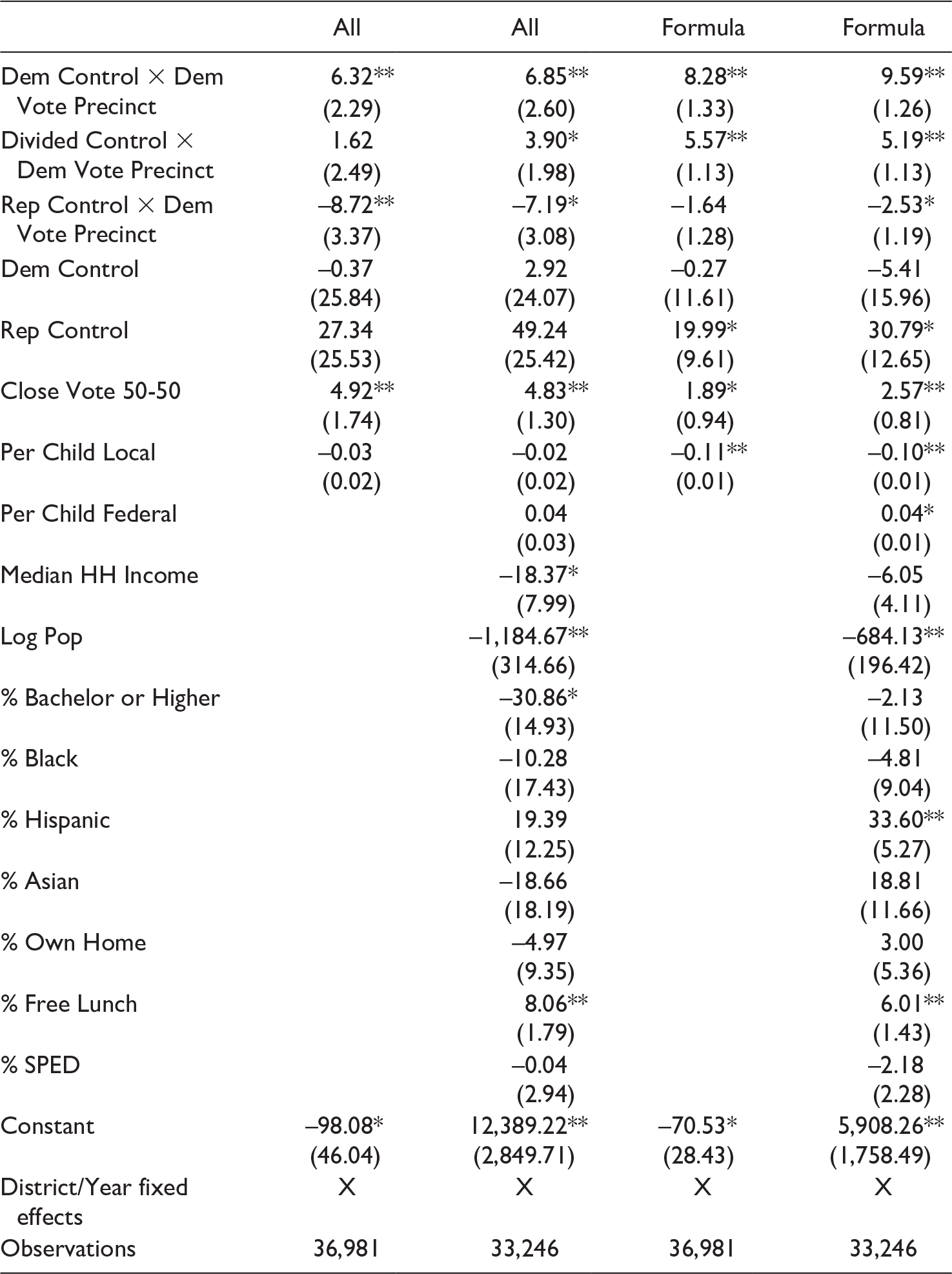
The first set of analyses answers the question, Do school districts that are more in line with the state-level government receive more in state transfers? Table 2 seeks to answer this question. The dependent variables in these models are the entire per child state transfer to the school district, relative to the state mean (columns 1 and 2), and the per child state transfer that comes through the funding formula, relative to the state mean (columns 3 and 4). Therefore, if Dem Vote Precinct × Dem Control is positive and significant, that would imply that when Democrats are in control at the state level, each percentage point in the two-party presidential vote for a Democrat that the school district voted above the state mean would result in an increase in money from the state.Footnote 11 Columns 1 and 3 contain a basic model with just key variables of interest. Columns 2 and 4 add the full set of covariates.
State Transfers and Party Control at School District Level.

Note. All refers to all state transfers; formula refers to transfers through the funding formula. Bootstrap standard errors are in parentheses. HH = household; % SPED = percentage enrolled in special education.
*p < .05. **p < .01.
In Table 2, Dem Control × Dem Vote Precinct is positive and significant across all four models, Divided Control × Dem Vote Precinct is positive and significant when focusing on transfers through the funding formula, and Rep Control × Dem Vote Precinct is negative and statistically significant in all but one model. Figure 3 plots the 95% confidence intervals for the key variables corresponding with columns 2 and 4 in Table 2. Even after controlling for local and federal contributions and district demographics, district partisan vote predicts transfers from the state to the district. It appears that both the overall transfers and transfers through the funding formula are susceptible to partisan influences. Interestingly, the closeness of the vote is statistically significant for all models as well. It is positive, indicating that the greater the margin of victory, the larger the transfer of funds.
District-level transfers and district two-party vote.
Note. The figure plots the 95% confidence intervals for party control and Democratic vote at the district level for Table 2. Two separate models are shown: all transfers and funding formula transfers (columns 2 and 4).

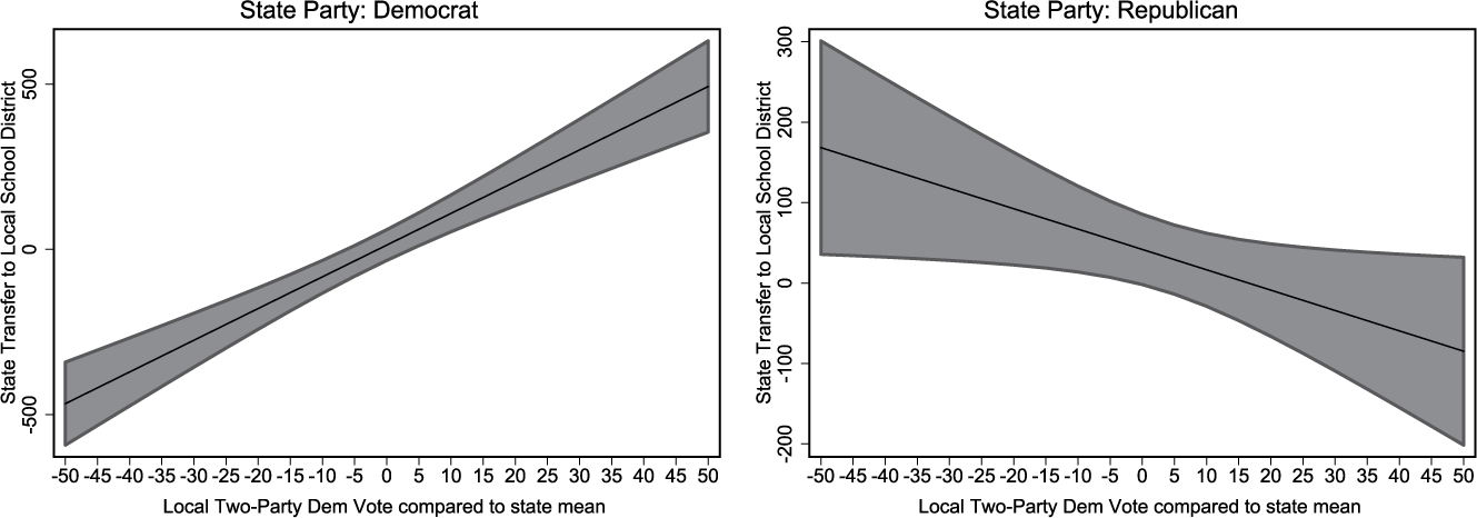
The effect of a marginal change in two-party vote on state funding formula transfers is plotted in Figure 4. The figure on the left plots the change when Democrats are in control at the state level and the figure on the right plots the change when Republicans are in control. While the relationship is much stronger for Democrats, both are in the expected direction. When Republicans have control at the state level, districts that support Republicans at higher rates still receive a boost. A 1 percentage point increase in support above the state mean while Democrats are in control at the state level is associated with $9.59 more per student in the state funding formula. When Republicans are in control, a 1 percentage point increase in support of Republicans above the state mean is associated with $2.53 more per student.
Effect of marginal change in district two-party vote on state transfers.
Note. The figures plot the effect of a marginal change in two-party Democratic vote within a district on the per child state transfer to the district, relative to the state mean. The left figure plots the change when Democrats are in control at the state level. The right figure plots the change when Republicans are in control at the state level. These figures correspond to column 4 of Table 2.

In terms of other covariates in the model, many follow the expected direction. An increase in median household income is associated with a decrease in state transfers to the district. An increase in the percentage of students receiving free or reduced lunch is associated with an increase in state transfers. Several variables are not related to the state transfer, including percentage that own a home or many of the measures of diversity. The one exception is percent Hispanic is related to the transfers through the funding formula. This could be explained by increased funding for programs to help English language learners.
One possible explanation for the partisan transfers is that parties have different priorities in funding education. Based on policy preferences, we might expect Democrats to focus on equity issues, such as increased funding to school districts with higher needs. For example, Democrats might target funding to areas that have a higher percentage of students on free and reduced lunch because this would help achieve their policy goal of improving education outcomes in high-poverty areas. Republicans have not made this a priority, so we would not expect them to direct funds in this way. Parties might also try to direct education funds to areas that are likely supporters, not just voters themselves. Black citizens vote for Democrats at significantly high rates than for Republicans. Democrats again might try to target funds to school districts that are more likely to support them. To test how different goals for education funding might matter, I run two additional models: (1) I interact state-level control with percent black within a district and (2) I interact state-level control with the percentage of students on free or reduced lunch within a district. These models will allow me to see whether Republicans and Democrats have different priorities in distributing funds.
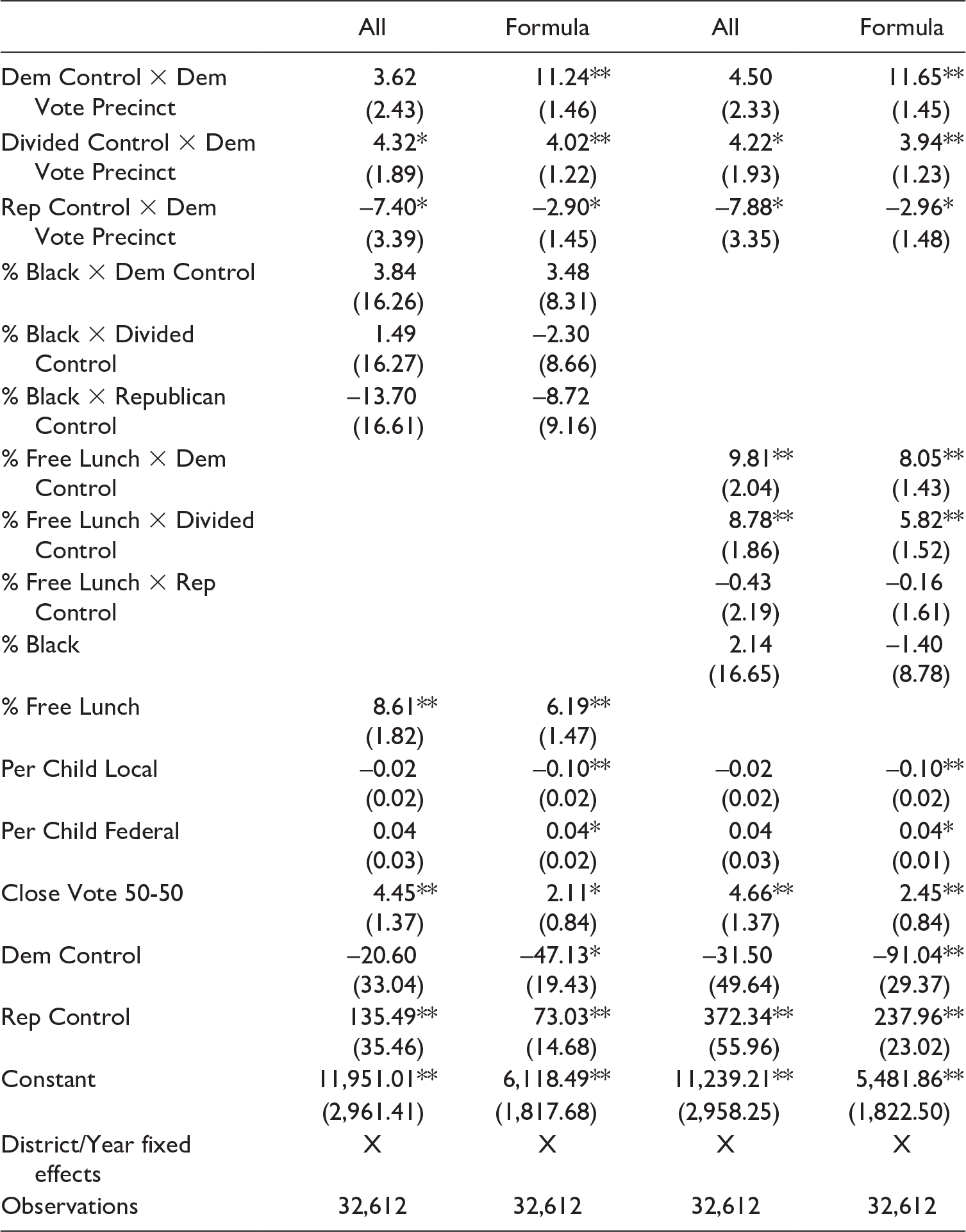
In addition to these new interactions, I also include the main interaction with district two-party vote. If Democrats are targeting areas that are likely to have high Democratic support or areas that they deem are in the most need and not Democratic voters themselves, then the coefficient for Dem Control × Dem Vote Precinct should no longer be statistically significant once these other variables are included in the model. Table 3 shows the results. Even after including this additional interaction, results hold. This suggests that after controlling for differences in preferences for distributing education funds, parties are still targeting their own voters in the funding formula.
State Transfers and Party Control at School District Level.

Note. The model also includes the following covariates not shown for space reasons: % Hispanic, % Asian, Log Pop, % SPED, Median HH Income, % Bachelor or Higher, and % Own Home. The results include district and year fixed effects. Bootstrap standard errors are in parentheses. Elections between 2000 and 2010 are included. HH = household income.
*p < .05. **p < .01.
Focusing on columns 1 and 2 first, the interactions between state-level party control and % Black are not statistically significant, but are in the expected direction. However, the main interaction between school district partisanship and state control is consistent with the previous model. The main exception is that the coefficient on Dem Vote Precinct × Dem Control for all state transfers is not statistically significant. However, it is for transfers through the funding formula. The coefficient on Dem Vote Precinct × Rep Control is negative and statistically significant in both models.
When focusing on columns 3 and 4, the main interaction between school district partisanship and state control is again consistent. State transfers are statistically related to partisan voting within a district. State transfers to areas of higher need, as measured by the percentage of free and reduced lunch students, are related to the party in control at the state level. The interaction term is positive and statistically significant for % Free Lunch × Dem Control but not % Free Lunch × Rep Control. This indicates that Democrats are also targeting areas of higher need, but we do not see the same effect when Republicans are in control.
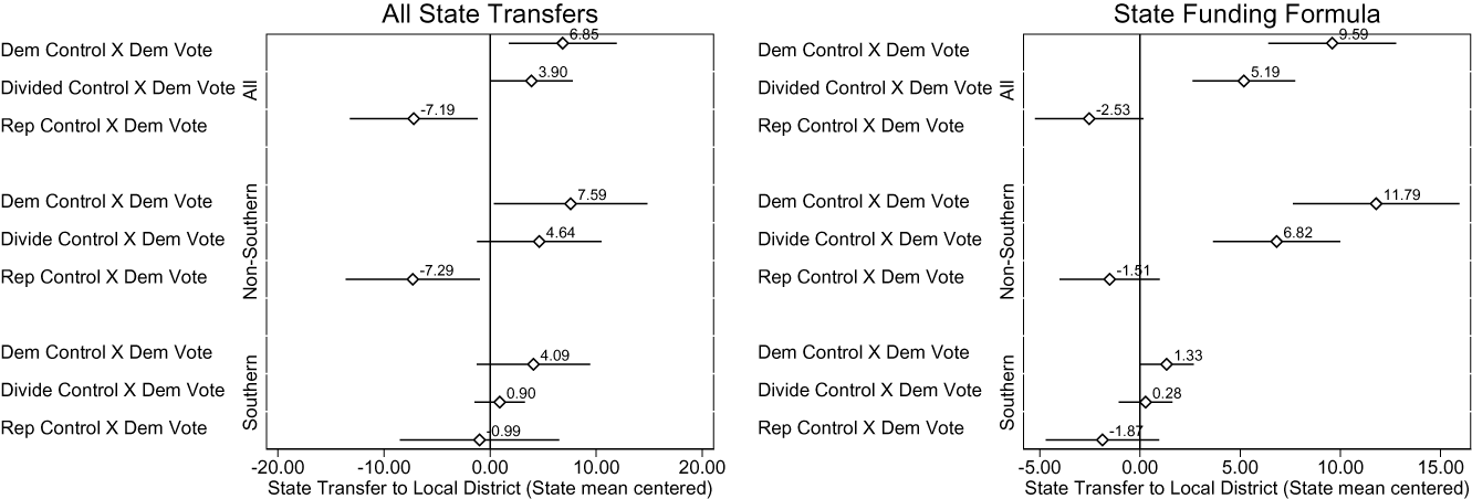
Republicans and Democrats can have different strategies for targeting funding, but there is variation from state to state in what it means to be a Democrat or a Republican, particularly when focusing on the South. The next set of analyses looks at the region of school district to see whether there are any differences in partisan transfers. In determining the ideological position of states, Shor and McCarty (Reference Shor and McCarty2011) found that the Democratic party in many Southern states was more conservative than the Republican party in other, non-Southern states. Figure 5 plots the key coefficients for three models: all states, non-Southern states, and Southern states for both all state transfers (left) and state funding formula (right).Footnote 12 Interestingly, there is little relationship between partisanship at the district level and state control in the South for all state transfers or transfers from the funding formula. For non-Southern states, the magnitude is slightly larger than the overall models. A 1 percentage point increase in voting for a Democrat when Democrats are in control is associated with a $7.59 increase in overall transfers and a $11.79 increase in transfers from the funding formula to the district in non-Southern states. Similarly, a 1 percentage point increase in voting for a Democrat when Republicans are in control is associated with a $7.29 decrease in overall transfers and a $1.51 decrease in transfers from the funding formula to the district in non-Southern states. The relationship is not statistically significant. It is possible that what it means to be a Democrat in the South has changed significantly during this time frame that it is not a good measure in the South.
Transfers by Southern versus non-Southern states.
Note. The figures plot the 95% confidence intervals for party control and presidential vote within the school district. Within each graph, three separate models are shown: all districts, districts not in the South, and districts in the South. The all district models correspond to columns 2 and 4 of Table 2. The Southern and non-Southern models include the same covariates, but are subset by region.

Robustness Checks
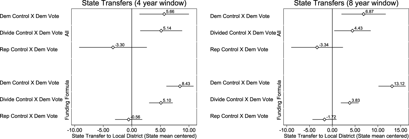
To ensure results are consistent, I run several different robustness checks. First, I test the window of state control. In the previous models, I used a time frame of party state control based on the budget cycle of that state (i.e., one or two years). However, some changes might take longer to implement. Therefore, I run additional models where I change the window to four years and eight years of state control. Results are consistent, although slightly smaller in magnitude. The image on the left in Figure 6 shows 95% of the key variables for each of the time frames. Both Dem Control × Dem Vote Precinct and Divided Control × Dem Vote Precinct are positive and significant when focusing on all transfers, and Rep Control × Dem Vote Precinct is negative but not significant.
Change window of state control.
Note. The figure plots the 95% confidence intervals for party control and Democratic vote at the district level. In the graph on the left, a four-year window of state control is used. In the graph on the right, an eight-year window of state control is used. The models include the same covariates and specification as in columns 2 and 4 of Table 2.

The next robustness check focuses on model specification. First, I change the standard errors. Instead of bootstrap standard errors, I use jackknife standard errors. The results are shown on the left in Figure 7. Results are consistent. Next, I focus on the way I model the state–district relationship. Instead of using fixed effects for school districts, I used a mixed model approach. In this model, I nest school districts within states and include random intercepts for both school districts and states. The graph on the right in Figure 7 displays the coefficients for the variables of interest. Results are very similar to the overall models, showing that the results are robust to modeling strategies.
Changing model specifications.
Note. The figures plot the 95% confidence intervals for party control and presidential vote within the school district. Instead of using fixed effects for school districts, a mixed model is used with school districts nested within states. The models include the same covariates as in columns 2 and 4 of Table 2.

Finally, I run models that uses district-level transfers but county-level two-party vote. While the two-party county vote masks variation in voting preferences between school districts within the same county, it is an approximation. In addition, I was able to collect more years of data for the county two-party vote than for precinct two-party vote. The years are expanded to 1992–2012 and include all states. Figure B.4 in Supplemental Appendix plots the 95% confidence intervals for the key variables. Again, results show a similar pattern but slightly larger in magnitude. The exception is that Rep Control × Dem Vote Precinct is positive. This indicates that this county level of data could be masking relationships that we find with more granular data.
Discussion and Conclusion
I have tested whether state party control influences distributions of state transfers to local school districts based on a core voter model. Previous research has found support for the core voter model when looking at total state transfers at the county level, but counties can include a wide variation of voters. I use school districts as a way to define more homogeneous groups of voters. While state funding formulas are often touted as a way to distribute money fairly, they are often not transparent and difficult to understand. This lack of transparency might make it easier for politicians to create formulas that would favor their constituents most likely to support them and not based on need. The results are consistent in that transfers to like constituents occur.
The results suggest that Democrats and Republicans act differently when in control at the state level. When looking at the overall transfers, the magnitude on the interaction terms is similar between the two parties. When focused on the funding formula itself, the magnitude is larger when Democrats are in control at the state level. Therefore, when Republicans are in control at the state level, they are possibly choosing to reward supporting districts with other types of funding for education not captured in the funding formula. Differences between the two parties are even more evident when looking at the interaction between state party control and percentage of students receiving free lunch. When Democrats are in control at the state level or it is divided control, more money is transferred to these districts with higher need. This is not the case when Republicans are in control at the state level. An increase in the percentage of students receiving free or reduced lunch is associated with no change in state transfers. But even after controlling for differential transfers based on need, I still find evidence of partisan transfers based on voting patterns. State politicians are strategic in getting resources to partisan voters. This article does not capture all education spending. This focuses specifically on transfers to traditional public schools. To further understand the differences in partisan influences, future research should capture transfers to local districts that include transfers to nontraditional public schools, like charter schools or voucher funding, to see whether partisanship preferences play a role here as well.
These results also suggest that the South is still distinctive. The relationship does not hold when looking at Southern states by themselves. While Ansolabehere and Snyder (Reference Ansolabehere and Snyder2006) did not look at Southern and non-Southern states separately, of the 13 states that they excluded for not changing party leadership during the time period they analyzed, 11 were Southern states.Footnote 13 The lack of findings in the South could be explained by an imprecise measure for support for Democratic candidates in this region. Most of the election voting are based on federal office, with the exception of the vote for governor. Democratic candidates at the federal level and Democratic candidates at the state level looked different during this time frame. Future work should address whether this is a measurement issue or whether the South is distinctive in other ways.
There are many implications for the distribution of funds for public education. As Hoxby (Reference Hoxby2001) notes, because funding formulas are based on local property taxes, the distributive nature is very different than other types of government transfers. The type of funding scheme selected can leave some districts, including poorer districts, worse off. It can also have effects beyond public school finance, including property prices, private school attendance, and student achievement. Increases in school funding are found to have strong, lasting effects. Jackson, Johnson, and Persico (Reference Jackson and Johnson2015) find that a 10% increase in per child spending in each year of schooling for all 12 years leads to more years of completed education, higher wages, and reduction in adult poverty. It is, therefore, important that all factors that influence the distribution of these goods be understood.
Declaration of Conflicting Interests
The author(s) declared no potential conflicts of interest with respect to the research, authorship, and/or publication of this article.
Funding
The author(s) received no financial support for the research, authorship, and/or publication of this article.
ORCID iD
Karin E. Kitchens https://orcid.org/0000-0003-4753-0730
Supplemental Material
Supplemental material for this article is available online.
Author Biography
Karin E. Kitchens is an assistant professor of Political Science at Virginia Tech.