
I. INTRODUCTION
Despite substantial insights provided by atomistic simulations over the past few decades into the basic mechanisms of metal plasticity, there is an important limitation to these techniques.Reference Abraham, Broughton, Bernstein and Kaxiras1,Reference McDowell2 Specifically, full atomistic models are impractical in simulating actual experiments of plastic deformation of metallic materials owing to the fact that dislocation pile-ups have long range stress fields that extend well beyond what can be captured using classical molecular dynamics (MD) and molecular statics (MS).Reference Bulatov, Abraham, Kubin, Devincre and Yip3,Reference Spearot and Sangid4 This has motivated researchers to develop partitioned-domain (or domain decomposition) multiscale modeling approaches that retain atomistic resolution in regions where explicit descriptions of nanoscale structure and phenomena are essential, while employing continuum treatment elsewhere.Reference Phillips5,Reference Tadmor and Miller6
One framework for such mixed continuum/atomistic modeling is the concurrent atomistic-continuum (CAC) method.Reference Xiong, Tucker, McDowell and Chen7 In a prototypical CAC simulation, a simulation cell is partitioned into a coarse-grained domain at continuum level and an atomistic domain,Reference Xu, Che, Xiong, Chen and McDowell8 employing a unified atomistic-continuum integral formulation of the governing equations with the underlying interatomic potential as the only constitutive relation in the system. The atomistic domain is updated in the same way as in an atomistic simulation while the coarse-grained domain contains elements that have discontinuities between them.Reference Chen, Zimmerman, Krivtsov and McDowell9 As such, CAC admits propagation of displacement discontinuities (dislocations and associated intrinsic stacking faults) through the lattice in both coarse-grained and atomistic domains.Reference Chen, Lee and Xiong10 Distinct from most partitioned-domain multiscale methods in the literature, the CAC method (i) describes certain lattice defects and their interactions using fully resolved atomistics; (ii) preserves the net Burgers vector and associated long range stress fields of curved, mixed character dislocations in a sufficiently large continuum domain in a fully 3D modelReference Xu11; (iii) employs the same governing equations and interatomic potentials in both atomistic and coarse-grained domains to avoid the usage of phenomenological parameters, essential remeshing operations, and ad hoc procedures for passing dislocation segments between the two domains.Reference Knap and Ortiz12,Reference Eidel and Stukowski13
In recent years, the CAC approach has been used as an effective tool for coarse-grained modeling of various nano/microscale thermal and mechanical problems in a wide range of monatomic and polyatomic crystalline materials. Important static properties of pure edge, pure screw, and mixed-type dislocations in metals, including the generalized stacking fault energy surface, dislocation core structure/energy/stress fields, and Peierls stress, have been benchmarked in the coarse-grained domain in CAC against atomistic simulations, and the trade-off between accuracy and efficiency in the coarse-graining procedure has been quantified.Reference Xu, Che, Xiong, Chen and McDowell8,Reference Xu, Xiong, Chen and McDowell14 The success of these calculations suggests the viability of using the CAC method to tackle more complex dislocation-mediated metal plasticity problems. Particularly for pure metals, CAC has been adopted to simulate surface indentation, quasistatic,Reference Xu, Che, Xiong, Chen and McDowell8 subsonic,Reference Xu, Xiong, Deng and McDowell15 and transonicReference Xiong, Rigelesaiyin, Chen, Xu, McDowell and Chen16 dislocation migration in a lattice, dislocations passing through the coarse-grained/atomistic domain interface,Reference Xu, Che, Xiong, Chen and McDowell8 screw dislocation cross-slip,Reference Xu, Xiong, Chen and McDowell17 dislocation/void interactions,Reference Xiong, Xu, McDowell and Chen18 dislocation/stacking fault interactions,Reference Xu, Xiong, Chen and McDowell19 dislocations bowing out from obstacles,Reference Xu, Xiong, Chen and McDowell20 dislocation multiplication from Frank–Read sources,Reference Xu, Xiong, Chen and McDowell14 sequential slip transfer of dislocations across grain boundaries (GBs),Reference Xu, Xiong, Chen and McDowell21,Reference Xu, Xiong, Chen and McDowell22 and brittle-to-ductile transition in dynamic fracture.Reference Xu, Xiong, Deng and McDowell15 It is shown that CAC provides largely satisfactory predictive results at a fraction of the computational cost of the fully atomistic version of the same models. While the net Burgers vector of dislocations is preserved in the coarse-grained domain, we remark that there exist coarse-graining errors in the dislocation description.Reference Xu, Che, Xiong, Chen and McDowell8 However, (i) these errors are not essential if the lattice defects are rendered in atomistic resolution because the dislocation will have a correct core structure once it migrates into the atomistic domain in which critical dislocation/defect interactions take placeReference Xu, Xiong, Chen and McDowell21,Reference Xu, Xiong, Chen and McDowell22 and (ii) even with fully coarse-grained models, CAC is useful for problems that do not require highly accurate full-field reproduction of atomistic simulations (e.g., large models).
In this article, we introduce PyCAC, a novel numerical implementation of the CAC approach. Written mostly in Fortran 2008, PyCAC is equipped with a Python scripting interface to create a more efficient, user-friendly, and extensible CAC simulation environment, which consists of a CAC simulator and a data analyzer. In the remainder of this paper, we start with the theoretical background of CAC in Sec. II. Next, we discuss the serial algorithms of dynamic, quasistatic, and hybrid CAC, along with some programming techniques in the PyCAC code in Sec. III. Then, we present the parallelization steps in the CAC simulator in Sec. IV and the PyCAC software in Sec. V. In the end, a summary and discussions of future research directions are provided in Sec. VI.
II. THEORETICAL BACKGROUND
The theoretical foundation of the CAC method is the atomistic field theory (AFT),Reference Chen and Lee23,Reference Chen24 which is an extension of the Irving–Kirkwood’s nonequilibrium statistical mechanical formulation of “the hydrodynamics equations for a single component, single phase system”Reference Irving and Kirkwood25 to a two-level structural description of crystalline materials. It employs the two-level structural description of all crystals in solid state physics, i.e., the well known equation of “crystal structure = lattice + basis”.Reference Kittel26 As a result of the bottom-up atomistic formulation, all the essential atomistic information of the material, including the crystal structure and the interaction between atoms, is built in the formulation. The result is a CAC representation of balance laws for both atomistic and continuum coarse-grained domains in the following formReference Chen and Lee23,Reference Chen24 :
 $${{{\rm{d}}{\rho ^\alpha }} \over {{\rm{d}}t}} + {\rho ^\alpha }\left( {{\nabla _{\bf{x}}} \cdot {\bf{v}} + {\nabla _{{{\bf{y}}^\alpha }}} \cdot \Delta {{\bf{v}}^\alpha }} \right) = 0\quad ,$$
 $${\rho ^\alpha }{{\rm{d}} \over {{\rm{d}}t}}\left( {{\bf{v}} + \Delta {{\bf{v}}^\alpha }} \right) = {\nabla _{\bf{x}}} \cdot {{\bf{t}}^\alpha } + {\nabla _{{{\bf{y}}^\alpha }}} \cdot {{\bf{\tau }}^\alpha } + {\bf{f}}_{{\rm{ext}}}^\alpha \quad ,$$
 $${\rho ^\alpha }{{{\rm{d}}{e^\alpha }} \over {{\rm{d}}t}} = {\nabla _{\bf{x}}} \cdot {{\bf{q}}^\alpha } + {\nabla _{{{\bf{y}}^\alpha }}} \cdot {{\bf{j}}^\alpha } + {{\bf{t}}^\alpha }:{\nabla _{\bf{x}}}\left( {{\bf{v}} + \Delta {{\bf{v}}^\alpha }} \right) + {{\bf{\tau }}^\alpha }:{\nabla _{{{\bf{y}}^\alpha }}}\left( {{\bf{v}} + \Delta {{\bf{v}}^\alpha }} \right)\quad ,$$
where x is the physical space coordinate; yα (α = 1, 2, …, N a with N a being the total number of atoms in a unit cell) are the internal variables describing the position of atom α relative to the mass center of the lattice cell located at x; ρα, ρα(v + Δvα), and ραe α are the local densities of mass, linear momentum, and total energy, respectively, where v + Δvα is the atomic-level velocity and v is the velocity field;  ${\bf{f}}_{{\rm{ext}}}^\alpha$ is the external force field; tα and qα are the stress and heat flux tensors due to the homogeneous deformation of lattice, respectively; τα and jα are the stress and heat flux tensors due to the reorganizations of atoms within the lattice cells, respectively; and the colon : denotes the scalar product of two second rank tensors A and B, i.e., A:B = A ijB ij.
For conservative systems, i.e., a system in the absence of an internal source that generates or dissipates energy, the energy equation [Eq. (3)] is equivalent to the linear momentum equation [Eq. (2)]. As a result, only the first two governing equations [Eqs. (1) and (2)] are explicitly implemented in the CAC simulator. Employing the classical definition of kinetic temperature, which is proportional to the kinetic part of the atomistic stress, the linear momentum equations can be expressed in a form that involves  ${\bf{f}}_{{\rm{ext}}}^\alpha$, internal force density
 ${\bf{f}}_{{\mathop{\rm int}} }^\alpha$, and temperature T,Reference Xiong, Chen and Lee27,Reference Xiong and Chen28
 $${\rho ^\alpha }{{{\ddot{\bf u}}}^\alpha }\left( {\bf{x}} \right) + {{{\gamma ^\alpha }{k_{\rm{B}}}} \over {\Delta V}}{\nabla _{\bf{x}}}T = {\bf{f}}_{{\mathop{\rm int}} }^\alpha \left( {\bf{x}} \right) + {\bf{f}}_{{\rm{ext}}}^\alpha \left( {\bf{x}} \right),\quad \alpha = 1,2, \ldots ,{N_{\rm{a}}}\quad ,$$
where uα is the displacement of the αth atom at point x, the superposed dots denote the material time derivative, ΔV is the volume of the finite-sized material particle (the primitive unit cell for crystalline materials) at x, k B is the Boltzmann constant, 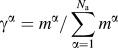 ${\gamma ^\alpha } = {m^\alpha }{\rm{/}}\sum\limits_{\alpha = 1}^{{N_{\rm{a}}}} {{m^\alpha }}$, T is the absolute temperature (in K), and
 ${\bf{f}}_{{\mathop{\rm int}} }^\alpha \left( {\bf{x}} \right)\left( { = {\nabla _{\bf{x}}} \cdot {{\bf{t}}^\alpha }} \right)$ is a nonlinear nonlocal function of relative atomic displacements. For systems with a constant temperature field or a constant temperature gradient, the temperature term in Eq. (4), which can be denoted as
 ${\bf{f}}_T^\alpha$, has the effect of a surface traction on the boundary or a body force in the interior of the material.Reference Xiong and Chen28 In the CAC simulator, the term
 ${\bf{f}}_T^\alpha$ has not yet been implemented because, as will be discussed in Sec. V.A, the current version of PyCAC can only simulate materials in a constant temperature field, in which case the effect of
 ${\bf{f}}_T^\alpha$ on mechanical properties is small. We remark that there is ongoing work in interpreting
 ${\bf{f}}_T^\alpha$ and in comparing different descriptions of temperature in the coarse-grained domainReference Chen29,Reference Chen and Diaz30 ; new understanding obtained will be implemented in future versions of PyCAC.
For monatomic crystals, yα = 0 and N a = 1; the governing equations in the physical space reduce to
 $${{{\rm{d}}\rho } \over {{\rm{d}}t}} + \rho {\nabla _{\bf{x}}} \cdot {\bf{v}} = 0\quad ,$$
 $$\rho {{{\rm{d}}{\bf{v}}} \over {{\rm{d}}t}} = {\nabla _{\bf{x}}} \cdot {\bf{t}} + {{\bf{f}}_{{\rm{ext}}}}\quad ,$$
 $$\rho {{{\rm{d}}e} \over {{\rm{d}}t}} = {\nabla _{\bf{x}}} \cdot {\bf{q}} + {\bf{t}}:{\nabla _{\bf{x}}}{\bf{v}}\quad ,$$
and, for conservative systems, in the absence of  ${\bf{f}}_T^\alpha$, Eq. (4) becomes
 $$\rho {{\ddot{\bf u}}} = {{\bf{f}}_{{\mathop{\rm int}} }} + {{\bf{f}}_{{\rm{ext}}}\quad .$$
Discretizing Eq. (8) using the Galerkin finite element method yields
 $$\int_{\Omega \left( {\bf{x}} \right)} {{\Phi _\xi }\left( {\bf{x}} \right)\left( {\rho {{\ddot{\bf u}}}\left( {\bf{x}} \right) - {{\bf{f}}_{{\mathop{\rm int}} }}\left( {\bf{x}} \right) - {{\bf{f}}_{{\rm{ext}}}}\left( {\bf{x}} \right)} \right){\rm{d}}{\bf{x}} = 0} \quad ,$$
where Ω is the simulation domain and Φξ is the finite element shape function. In the coarse-grained domain, the integral in Eq. (9) can be evaluated using numerical integration methods such as Gaussian quadrature. It is, however, difficult to employ a unified set of integration points within an element because the internal force density fint can be a complicated and highly nonlinear function of x, whose order and distribution are usually difficult to anticipate a priori.Reference Xu, Che, Xiong, Chen and McDowell8,Reference Xu11 To circumvent this problem, we divide each element into a number of nonoverlapping subregions, whose order is usually lower than that within the entire element and is thus more easily approximated. In the CAC simulator, within each subregion, the first order Gaussian quadrature with one integration point at the center of the subregion is adopted; then the integrals of all subregions within an element are summed, resulting in the force on node ξ asReference Xu, Che, Xiong, Chen and McDowell8
 $${{\cal F}^\xi } = {{\sum\limits_\mu {{\omega _\mu }{{\bf{\Phi }}_{\mu \xi }}{{\bf{F}}^\mu }} } \over {\sum\limits_\mu {{\omega _\mu }{{\bf{\Phi }}_{\mu \xi }}} }} + {\bf{F}}_{{\rm{ext}}}^\xi \quad ,$$
where ωμ is the weight of integration point μ, Φμξ is the shape function of node ξ at integration point μ, Fμ is the interatomic potential-based atomic force on integration point μ, and  ${\bf{F}}_{{\rm{ext}}}^\xi$ is the external force applied on node ξ. Once the nodal positions are determined, the positions of atoms within an element are interpolated from those of the nodes using the shape function Φ; in other words, all elements are isoparametric.
In the atomistic domain, an atom can be viewed as a special finite element for which the shape function reduces to 1 at the atomic site, and the force on atom α is simply
 $${{\bf{F}}^\alpha } = - {\nabla _\alpha }E + {\bf{F}}_{{\rm{ext}}}^\alpha \quad ,$$
where E is the interatomic potential-based internal energy and  ${\bf{F}}_{{\rm{ext}}}^\alpha$ is the external force applied on atom α. The CAC method, as a coarse-grained atomistic methodology, reduces to standard MD or MS if only fully resolved atomistic domains are considered in the simulation, in which case Eq. (10) is no longer relevant and only Eq. (11) takes effect. In other words, the PyCAC code is capable of performing fully-resolved MD/MS simulations if only atoms are involved. In the remainder of this paper, both
 ${\cal F}$ and F are referred to in combination as F.
III. SERIAL ALGORITHMS
While the CAC simulator runs in parallel, we focus on the serial algorithms of the CAC simulator and the data analyzer in this section to elucidate their differences from atomistic methods. The parallelization steps in the CAC simulator will be detailed in Sec. IV.
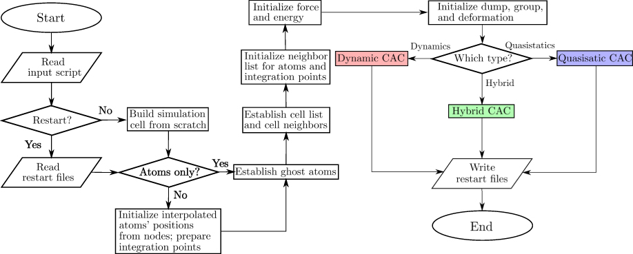
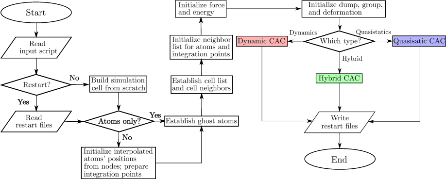
Similar to the MD and MS methods in atomistic simulations, users of PyCAC can choose among dynamic CAC, quasistatic CAC, and hybrid CAC, as illustrated in the serial CAC simulation scheme (Fig. 1). In all CAC simulations, the nodes in the coarse-grained domain and the atoms in the atomistic domain interact with each other at each simulation step and are updated concurrently.
Serial CAC simulation scheme.
A. Dynamic CAC
In dynamic CAC, the forces F are used in the equation of motion
 $$m{{\ddot{\bf R}}} = {\bf{F}}\quad ,$$
or its modified version, where m is the normalized lumped or consistent mass in the coarse-grained domain or the atomic mass in the atomistic domain and R is the nodal/atomic position. Three options are provided: velocity Verlet (vv), quenched dynamics (qd), and Langevin dynamics (ld), as illustrated in Fig. S1 (Supplementary Material).
For both vv and qd options, Eq. (12) is solved with the velocity Verlet algorithmReference Swope, Andersen, Berens and Wilson31; with qd, the nodal/atomic velocities  ${{\dot{\bf R}}}$ are also adjusted by nodal/atomic forces F following the “quick-min” MD approachReference Sheppard, Terrell and Henkelman32 to force the system energy toward a minimum at 0 K,Reference Xu, Xiong, Chen and McDowell21,Reference Xu, Xiong, Chen and McDowell22 i.e.,
 $${{\dot{\bf R}}} = \left\{ {\matrix{ {{\bf{0}},} & {{\rm{if}}\;{{\dot{\bf R}}} \cdot {\bf{F}} \lt 0} \cr {{{\left( {{{\dot{\bf R}}} \cdot {\bf{F}}} \right){\bf{F}}} \over {{{\left| {\bf{F}} \right|}^2}}},} & {{\rm{otherwise}}} \cr} } \right.\quad .$$
With the ld option, which is used to keep a constant finite system temperature,Reference Xu, Xiong, Deng and McDowell15,Reference Xu, Xiong, Chen and McDowell17 Eq. (12) is extended by two terms, i.e.,
 $$m{{\ddot{\bf R}}} = {\bf{F}} - \gamma m{{\dot{\bf R}}} + \Theta \left( t \right)\quad ,$$
where γ is the damping coefficient with a unit of frequency and Θ(t) is the time-dependent Gaussian random variable with zero mean and variance of  $\sqrt {2m\gamma {k_{\rm{B}}}T{\rm{/}}\Delta t}$, where k B is the Boltzmann constant and Δt is the time step. Numerically, both Eqs. (12) and (14) are solved using the velocity Verlet formulation of the Brünger–Brooks–Karplus integrator.Reference Brünger, Brooks and Karplus33 In particular, when T = 0 K, Eq. (14) becomes damped MD, which is used for dynamic relaxation at near 0 K temperature.
In the early version of the AFT formulation,Reference Chen and Lee23 the local densities were defined as ensemble averages following the Irving–Kirkwood formulations,Reference Irving and Kirkwood25 and hence, the governing equations were written in terms of ensemble-averaged local densities. In the later version of the AFT formulation,Reference Chen24 the local densities are instantaneous quantities.Reference Evans and Morriss34 Consequently, the ensembles in AFT (and CAC) differ from other statistical mechanical formulations that follow the Gibbs’ equilibrium statistical theory of ensembles. Popular equilibrium ensembles include (i) the microcanonical ensemble, which describes a system isolated from its surroundings and governed by Hamilton’s equations of motion (NVE), (ii) the canonical ensemble, which describes a system in constant contact with a heat bath of constant temperature (NVT), and (iii) the isothermal–isobaric ensembles, which describe systems in contact with a thermostat at temperature T and a barostat at pressure P (NPT).Reference Tuckerman35 These ensembles, known as equilibrium ensembles and allowing a wide variety of thermodynamic and structural properties of systems to be computed, can be realized in dynamic CAC, in which a finite temperature can be achieved via lattice dynamic-based shape functions.Reference Chen, Diaz, Xiong, McDowell and Chen36 Alternatively, in the current code, a Langevin thermostat is realized using the ld option while a constant pressure/stress is maintained via a Berendsen barostatReference Berendsen, Postma, van Gunsteren, DiNola and Haak37; other thermostat and barostat may also be implemented.
Prior dynamic CAC applications using the vv option include phase transitions,Reference Xiong and Chen28 crack propagation and branching,Reference Deng, Xiong and Chen38,Reference Deng and Chen39 nucleation and propagation of dislocations,Reference Xiong, Tucker, McDowell and Chen7,Reference Xiong, Rigelesaiyin, Chen, Xu, McDowell and Chen16,Reference Xiong and Chen40–Reference Yang, Xiong, Deng and Chen42 formation of dislocation loops,Reference Xiong, McDowell and Chen43 defect/interface interactions,Reference Yang, Zhang and Chen44,Reference Yang and Chen45 phonon/dislocation interactions,Reference Xiong, McDowell and Chen46,Reference Chen, Xiong, McDowell and Chen47 and phonon/GB interactionsReference Chen, Li, Xiong, Li, Yang, Zheng, McDowell and Chen48,Reference Chen, Li, Diaz, Li, Chen and McDowell49 ; prior dynamic CAC simulations using the ld option include dislocation/void interactionsReference Xiong, Xu, McDowell and Chen18 (T ≈ 0 K), dislocation migrationReference Xu, Xiong, Deng and McDowell15 (T ≈ 0 K), and screw dislocation cross-slipReference Xu, Xiong, Chen and McDowell17 (T = 10 K). These simulations have revealed the underlying mechanisms for a variety of experimentally observed phenomena, including, but not limited to, phonon focusing, phonon-induced dislocation drag, phonon scattering by interfaces and by other phonons, co-existence of the coherent and incoherent propagation of ultrafast heat pulses in polycrystalline materials, and Kapitza thermal boundary resistance.
B. Quasistatic CAC
In quasistatic CAC, which is analogous in character to MS, F is used to systematically adjust the nodal/atomic positions at each increment of system loading during the energy minimization.Reference Xu, Che, Xiong, Chen and McDowell8 Four energy minimization algorithms are introduced: conjugate gradient (cg), steepest descent (sd), quick-min (qm), and fast inertial relaxation engine (fire), as illustrated in Fig. S2 (Supplementary Material). The energy minimization procedure stops when either the number of iterations reaches a maximum value or the energy variation between successive iterations divided by the current energy is less than a tolerance. Here, the “energy” consists of the interatomic potential-based internal energy E and the traction boundary conditions-induced external energy.
Both cg and sd algorithms follow the standard procedure in MS, which contains an outer iteration to find the search direction and the inner iteration to determine the step size.Reference Chapra and Canale50 For the qm and fire algorithms, there is no inner iteration. Instead, dynamic-like runs are iteratively performed at each loading increment until the energy converges. The qm algorithmReference Sheppard, Terrell and Henkelman32 is based on quenched dynamics, which is also used in dynamic CAC, except that in the latter case, only one quenched dynamics iteration is carried out at each simulation step. The fire algorithm is based on a local atomic structure optimization algorithm.Reference Bitzek, Koskinen, Gähler, Moseler and Gumbsch51,Reference Eidel, Hartmaier, Gumbsch, Gumbsch and Pippan52
A comparison of these four algorithms was presented by Sheppard et al.Reference Sheppard, Terrell and Henkelman32 In general, the cg algorithm is the most commonly used in atomistic simulationsReference Tadmor and Miller53 and has been used in several quasistatic CAC simulations,Reference Xu, Che, Xiong, Chen and McDowell8,Reference Xu, Xiong, Chen and McDowell14,Reference Xu, Xiong, Chen and McDowell19,Reference Xu, Xiong, Chen and McDowell20 while the fire algorithm is considered the fastest in certain cases.Reference Bitzek, Koskinen, Gähler, Moseler and Gumbsch51
C. Hybrid CAC
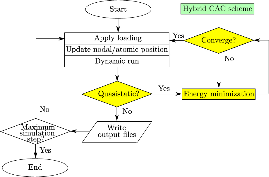
Besides the dynamic CAC and quasistatic CAC, the CAC simulator provides a third option: “hybrid CAC”, which allows users to perform periodic energy minimization during a dynamic CAC simulation, as illustrated in Fig. 2. Users can choose among all three dynamic options and four energy minimization algorithms. Hybrid CAC has been used in Refs. Reference Xu, Xiong, Chen and McDowell21 and Reference Xu, Xiong, Chen and McDowell22 to simulate dislocation pile-ups across GBs: a series of dislocations migrate and interact with GBs during the quenched dynamic run, while the fully relaxed GB structures, important in predicting accurate dislocation/GB interaction mechanisms, are obtained via periodic energy minimization using the conjugate gradient algorithm. In practice, this enables the multiscale optimization for a sequence of constrained nonequilibrium states (defect configurations) in materials.Reference Xu11 Accordingly, hybrid CAC yields results similar to quasistatic CAC at lower computational cost because the quenched dynamic run, which pertains to 0 K (or very nearly so), is more efficient than the conjugate gradient algorithm.Reference Xu, Xiong, Chen and McDowell21
Serial hybrid CAC simulation scheme. The quasistatic CAC procedures are highlighted in yellow, while the remaining procedures belong to the dynamic CAC simulation scheme. At the diamond box with “Quasistatic?”, the code decides, based on some user-defined input parameters, whether it switches from dynamic run to quasistatic run.

D. Programming techniques
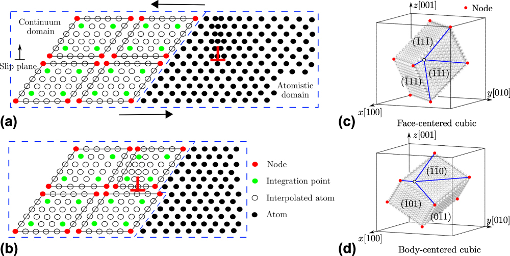
A framework for mixed atomistic/continuum modeling, the CAC algorithm adopts common finite element and atomistic modeling techniques. In the coarse-grained domain, the Garlekin method and Gaussian quadrature are used to solve Eq. (9).Reference Xu, Che, Xiong, Chen and McDowell8 To admit dislocation nucleation and migration, 3D rhombohedral elements with faces on {111} planes in a face-centered cubic (FCC) lattice or {110} planes in a body-centered cubic (BCC) lattice are used, as shown in Fig. 3. Within each element, lattice defects are not allowed and the displacement field has C1 continuity.Reference Xu, Che, Xiong, Chen and McDowell8 Between elements, however, neither displacement continuity nor strain compatibility is required. In this way, lattice defects are accommodated by discontinuous displacements between elements, potentially including both sliding and separation.Reference Xu11
(a, b) A 2D CAC simulation domain consisting of an atomistic domain (right) and a continuum domain (left).Reference Xu, Che, Xiong, Chen and McDowell8 In (a), an edge dislocation (red ⊥) is located in the atomistic domain. Upon applying a shear stress on the simulation cell, the dislocation migrates into the continuum domain in (b), where the Burgers vector spreads out between discontinuous finite elements. (c, d) In 3D, elements have faces on {111} planes and on {110} planes in an FCC and a BCC lattice, respectively. The positions of atoms (open circles) within each element are interpolated from the nodal positions (filled circles).

In the atomistic domain, Newton’s third law is used to promote efficiency in calculating the force, pair potential, local electron density, and stress. In addition, due to the similarity between CAC and atomistic methods regarding the crystal structure and force/energy/stress calculations, the short-range neighbor search employs a combined cell listReference Allen and Tildesley54 and Verlet listReference Verlet55 method. The neighbor lists, of the integration points in the coarse-grained domain and of the atoms in the atomistic domain, are updated on-the-fly when any node/atom is displaced by a distance that is larger than half a user-defined bin size. Displacement, traction, or mixed boundary conditions can be realized by assigning a displacement and/or force to the nodes/atoms within a short distance from the simulation cell boundaries. However, CAC with the present coarse-graining strategy differs from standard atomistic methods in five main aspects as follows:
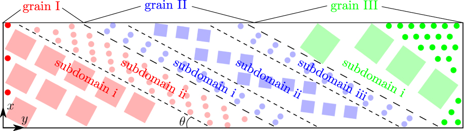
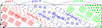
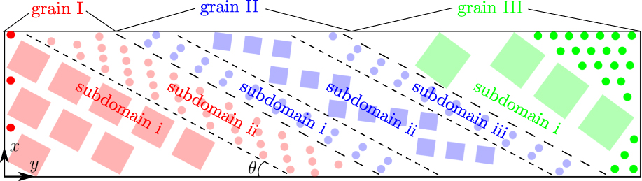
(i) The rhombohedral element shape and the fact that the finite elements may take any crystallographic orientations with respect to a fixed coordinate system prevent one from constructing a parallelepipedonal coarse-grained domain. To facilitate application of the periodic boundary conditions (PBCs), one can fill in the otherwise jagged interstices at simulation cell boundaries with atoms, e.g., the dark red and dark green circles in Fig. 4 since in this example, PBCs are applied along the y direction.
(ii) The other issue in implementing PBCs is that an object crossing through one face of the simulation cell should enter the cell through the opposite face. In atomistic simulations, this is realized via displacement of certain atoms to bring them back inside the cell,Reference Tadmor and Miller6 i.e.,
 $${R^\chi } = \left\{ {\matrix{ {{R^\chi } + {L^\chi },} & {\rm{i}{\rm{f}}\;{\it R^\chi } \lt \it R_{{\rm{lb}}}^\chi } \cr {{R^\chi } - {L^\chi },} & {\rm{i}{\rm{f}}\;{\it R^\chi } > \it R_{{\rm{ub}}}^\chi } \cr} } \right.\quad ,$$
where R χ is the position of an atom along the χ direction, L χ,  $R_{{\rm{lb}}}^\chi$, and
 $R_{{\rm{ub}}}^\chi$ are the length, lower boundary, and upper boundary of the simulation cell along the χ direction, respectively. In the coarse-grained domain, however, care must be taken when not all nodes of one element are displaced, i.e., an element is cut through by a periodic boundary.Reference Xu11 In this case, the nodal positions should be reinstated to interpolate the positions of atoms within the element. Subsequently, the reinstated nodes and some of the interpolated atoms are displaced following Eq. (15). More details of this procedure can be found in Appendix C of Ref. Reference Xu, Che, Xiong, Chen and McDowell8.
(iii) Compared with the two-body Lennard-Jones (LJ) pair potential,Reference Jones56 the many-body embedded-atom method (EAM) potentialReference Daw and Baskes57 adopts a more complicated formulation for the force F, i.e.,Reference Daw and Baskes57
 $${{\bf{F}}^k} = \sum\limits_{\matrix{ j \cr {j \ne k} \cr} } {\left\{ {{{\partial \phi \left( {{R^{kj}}} \right)} \over {\partial {R^{kj}}}} + \left[ {{{\partial \psi \left( {{{\bar{\rho }}^k}} \right)} \over {\partial {{\bar{\rho }}^k}}} + {{\partial \psi \left( {{{\bar{\rho }}^j}} \right)} \over {\partial {{\bar{\rho }}^j}}}} \right]{{\partial \rho \left( {{R^{kj}}} \right)} \over {\partial {R^{kj}}}}} \left\}{{{{\bf{R}}^{kj}}} \over {{R^{kj}}}}} \quad ,$$
where ϕ is the pair potential, ψ is the embedding potential,  $\bar{\rho }$ is the host electron density, and Rkj is the vector from atom k to atom j with norm R kj, i.e.,
 $${{\bf{R}}^{kj}} = {{\bf{R}}^j} - {{\bf{R}}^k}\quad ,$$
 $${\bar{\rho }^k} = \sum\limits_{\matrix{ j \cr {j \ne k} \cr} } {{\rho ^{kj}}\left( {{R^{kj}}} \right)} \quad ,$$
where ρ is the local electron density contributed by atom j at site k.
A 2D schematic of the grains and subdomains in a CAC simulation cell. Squares are finite elements and circles are atoms. In grain I, there are two subdomains; subdomain i contains elements of the same size while subdomain ii is fully atomistically resolved. In grain II, there are three subdomains; subdomains i and iii have full atomistic resolution, while subdomain ii contains elements of the same size. In grain III, there is only one subdomain containing elements of the same size. The elements are rotated differently in three grains following their respective crystallographic orientations. Note that the dark red and dark green atoms at the leftmost and rightmost boundaries are added after all grains/subdomains are defined, to fill in the otherwise jagged interstices at the periodic boundaries because PBCs are applied along the y direction but not the x direction. Also note that the planar interface between grains and subdomains are not necessarily normal to the Cartesian axes but can have a user-defined orientation angle θ.
In the atomistic domain, with the neighbor lists established for all atoms, the host electron densities  $\bar{\rho }$ of all atoms are first calculated using Eq. (18), followed by the calculation of the atomic forces F of all atoms using Eq. (16), with the aid of Newton’s third law in both calculations. In the coarse-grained domain, however, only the integration points have a neighbor list. On the other hand, in calculating the force on one integration point k using Eq. (16), one needs to know the host electron density
 ${\bar{\rho \,}^j}$ of its neighbors j, any of which, according to Eq. (18), requires a neighbor list for atom j, which may not be an integration point and does not naively have a neighbor list. Thus, the direct calculation of all
 ${\bar{\rho \,}^j}$ would require the establishment of neighbor lists for a lot of nonintegration-point atoms and would include a significant number of repeated computations because the atoms involved are located in close proximity. We found that this is computationally expensive, especially so in a large element with sparse integration points.Reference Xu11 Therefore, an approximation is introduced that within one element,
 $\bar{\rho }$ of all interpolated atoms in one subregion is assumed equal to that of the integration point in the same subregion.Reference Xu, Che, Xiong, Chen and McDowell8 In this way, one needs only to calculate
 $\bar{\rho }$ of the integration points, increasing the efficiency substantially. It was found that this approximation only slightly affects the dislocation configuration while retaining the overall Burgers vector.Reference Xu, Che, Xiong, Chen and McDowell8 Note that this approximation does not apply to the simple LJ pair potential since it does not involve the electron density.
(iv) As mentioned in Sec. I, a CAC simulation cell generally consists of a coarse-grained domain and an atomistic domain, with the elements and atoms constructed following different crystallographic orientations in different grains. Elements of different sizes may exist in the coarse-grained domain. Within one grain, to distinguish between atoms and elements as well as between elements of different sizes, the term “subdomain” is introduced to refer to a region in a CAC simulation cell with only atoms or only elements of the same size, as illustrated in Fig. 4. Users can build single crystal, bicrystal, or polycrystal models with any number of subdomains and/or grains that are stacked along any Cartesian axis, e.g., the y axis in Fig. 4. The planar interface between grains and subdomains is not necessarily normal to the Cartesian axes but can have a user-defined orientation exhibited by the tilt angle θ in Fig. 4.
(v) The last issue lies in the visualization of the CAC results, which is supported by the data analyzer. Naturally, both the real atoms in the atomistic domain and the interpolated atoms in the coarse-grained domain can be visualized in the same way as in the atomistic simulations using common atomistic configuration viewers such as OVITO,Reference Stukowski58 AtomEye,Reference Li59 VMD,Reference Humphrey, Dalke and Schulten60 and AtomViewer.Reference Begau, Hartmaier, George and Pharr61,Reference Begau, Hua and Hartmaier62 Unfortunately, these atomistic viewers do not naively support finite elements. Thus, we are in need of software that can concurrently render both elements and atoms as well as some nodal/atomic quantities such as energy, force, velocity (not for quasistatic CAC), and stress. For this purpose, the CAC simulator outputs vtk files for both elements and atoms, which can be visualized in the freely available software package ParaView,Reference Schroeder, Martin and Lorensen63 such that CAC results are accessible to a larger community.
IV. PARALLELIZATION
A. Parallel algorithm
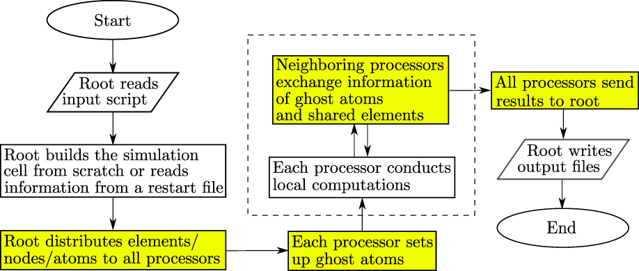
CAC simulations employ a distributed-memory parallel algorithm using the Message Passing Interface (MPI).Reference Gropp, Hoefler, Thakur and Lusk64 Among the three parallel algorithms commonly used in atomistic simulations—atom decomposition (AD), force decomposition (FD), and spatial decomposition (SD), SD yields the best scalability and the smallest communication overhead between processors and is therefore used in the CAC simulator.Reference Xu11 At each simulation step, all atoms in the coarse-grained domain are interpolated from the nodal positions, enabling the employment of the same parallel atomistic algorithm used in the state-of-the-art atomistic modeling software LAMMPS.Reference Plimpton65 In SD, each processor occupies a domain, with a certain number of local atoms. However, not all atoms that are within the interatomic potential cutoff distance of the local atoms are in the same processor domain. To address this problem, each processor domain is expanded outwards along the three Cartesian axes by a distance that equals the sum of the cutoff distance and a user-defined bin size; the atoms within the expanded regions are termed “ghost atoms”. Then, real-time positions of the ghost atoms are exchanged between neighboring processors at each step, with the Newton’s third law–induced numerical complication in the atomistic domain properly handled. The position of each node in the coarse-grained domain is also updated in this process because it is the center of mass of all atoms at that node, which is simply the atomic position at that node for monatomic crystals. Note that the ghost atoms are deleted and recreated every time the neighbor lists are updated. We emphasize that the ghost atoms, widely used in SD-based parallel atomistic simulations, are not related in any way to the “ghost force” at the continuum/atomistic domain interface in some multiscale modeling approaches, e.g., the local QC methodReference Tadmor, Ortiz and Phillips66; there is no ghost force in both undeformed and affinely deformed perfect lattices in CAC because all the nodes/atoms are nonlocal. The parallel CAC simulation scheme is presented in Fig. 5.
Parallel CAC simulation scheme. Procedures that do not exist in the serial scheme (Fig. 1) are highlighted in yellow. Note that (i) in the serial scheme, the root processor does everything and (ii) the two procedures in the dashed box are conducted back and forth until the output begins.

Unlike AD and FD, the workload of each processor in SD, which is proportional to the number of interparticle interactions, is not guaranteed to be the same. On the one hand, in parallel computing, it is important to assign processors approximately the same workload which, in CAC simulations, is the calculation of force, energy, stress, position, velocity (not for quasistatic CAC), and electron density (only for the EAM potential). On the other hand, in CAC, the simulation cell has nonuniformly distributed integration points in the coarse-grained domain and atoms in the atomistic domain, such that the workload is poorly balanced if one assigns each processor an equally sized cubic domain as in full atomistics.Reference Pearce, Gamblin, de Supinski, Arsenlis and Amato67 Thus, it is desirable to employ an algorithm to address the workload balance issue, which is not unique to CAC but is also encountered by other partitioned-domain multiscale modeling methods with highly heterogeneous models.Reference Pavia and Curtin68,Reference Biyikli and To69
In parallel CAC simulations involving both coarse-grained and atomistic domains, only the force/energy/host electron density (the last quantity pertains only to the EAM potential) of the integration points and atoms (referred to in combination as “evaluation points”) are computed. Since the local density of interactions does not vary significantly within the simulation cell, the number of evaluation points is used as an approximation of the workload and each processor domain is assigned approximately the same number of evaluation points, which is re-evaluated at regular time intervals.Reference Xu11 It follows that at periodic boundaries filled in with atoms or in the vicinity of lattice defects where full atomistics is used, the processors are assigned smaller domains that contain more atoms than other processors whose domains contain more elements.Reference Xu, Che, Xiong, Chen and McDowell8
Another issue that does not exist in parallel atomistic simulations but requires special attention in parallel finite element implementations is that in the latter, some elements may be shared between neighboring processors.Reference Xu11 In CAC, this issue originates from the difference in shape between the parallelepipedonal processor domain and the rhombohedral finite elements with arbitrary crystallographic orientations, the latter of which also results in the jagged simulation cell boundaries, as discussed in Sec. III.D. Instead of having all relevant processors calculate the same quantities within a shared element, in the CAC simulator, each relevant processor only calculates quantities of the integration points its domain contains; then these quantities are summed and sent to all relevant processors. This simple summation is feasible because of the trilinear shape function used in the finite elements.Reference Xu, Che, Xiong, Chen and McDowell8 Particular attention must be paid in the cases of (i) the EAM potential, where the host electron density approximation (Sec. III.D) should be correctly implemented because a subregion within an element may also be shared between processors and (ii) the Langevin dynamics, where different processors may have different Θ(t) [Eq. (14)] for the nodes of the same shared element because Θ(t) is a processor-dependent random variable; in practice, for a shared element, Θ(t) for the same node is averaged among all relevant processors. Distinct from atomistic simulations, each relevant processor needs to have the same copy of nodal positions of all its shared elements in its local memory to correctly interpolate its integration points’ and atoms’ neighbors. In practice, this leads to a lower parallel scalability and a poorer memory usage scaling than full atomistics.
We remark that in the CAC simulator, the input and output parts are not fully parallelized. Instead, following LAMMPS,Reference Plimpton65 the input script is first read by the root processor, which then builds the simulation cell from scratch or reads necessary information from a restart file. The simulation cell information is stored in some global arrays accessible only to the root processor. It follows that the root processor distributes all elements/nodes/atoms to all processors (including the root itself), which store the relevant data in local arrays and conduct local computations. For the output, all processors (including the root processor) send their local results to some global arrays accessible only to the root processor, which then writes the information to the file system. All global arrays are eliminated as soon as they are used to minimize the memory usage.
B. Parallel scalability
The primary motivation for developing the CAC method, or any partitioned-domain multiscale modeling method, is to run simulations at a cost lower than that of the full atomistic method. In our early work, the coarse-graining efficiency—the serial runtime of a full coarse-grained CAC simulation divided by that of an equivalent full atomistic simulation—was found to be about 50 when all elements are of second nearest neighbor (2NN) type and each contains 9261 atoms.Reference Xu, Che, Xiong, Chen and McDowell8 It was also found that the coarse-graining efficiency for a quasistatic run is higher than that of a dynamic run.Reference Xu, Che, Xiong, Chen and McDowell8
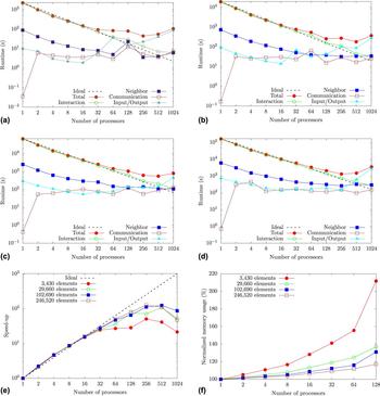
In this section, we conduct benchmark simulations to analyze the CAC simulator’s parallel scalability. There are two basic ways to measure the parallel scalability of a given application: strong scaling and weak scaling.Reference Hunter, Saied, Le and Koslowski70 As the number of processors increases, the problem size (e.g., number of elements/atoms in a simulation cell) remains the same in strong scaling but increases proportionally in weak scaling to keep a constant problem size per processor. Consequently, each processor communicates the same/smaller amount of data with its neighbors in weak/strong scaling, respectively. In this section, we investigate both strong (Fig. 6) and weak (Fig. 7) scaling of the CAC simulator by conducting fully coarse-grained simulations in Ni single crystals. To further analyze the parallel performance, the total runtime of each job is partitioned into four components: the time for interatomic interactions, the time for establishing/updating neighbors, the time for interprocessor communication, and the time for input/output. Each runtime component is calculated by averaging the corresponding component among all processors. The memory usage and processor workload are also analyzed. All simulations run on the Bridges cluster, with a peak speed of 1.35 petaflops per second, at National Science Foundation (NSF) Extreme Science and Engineering Discovery Environment (XSEDE).Reference Towns, Cockerill, Dahan, Foster, Gaither, Grimshaw, Hazlewood, Lathrop, Lifka, Peterson, Roskies, Scott and Wilkins-Diehr71 In each simulation, up to 1024 processors are used on Hewlett Packard Enterprise Apollo 2000 servers using 2.30 GHz Intel Xeon E5-2695 v3 CPUs with 35 MB cache size and Intel Omni-Path Fabric interconnection. Each node has 2 CPUs (14 cores per CPU), 128 GB RAM, and 8 TB storage. We emphasize that the simulations conducted here are solely for the purpose of code performance analysis and are not intended to shed light on any realistic material response.
(a–d) Runtime breakdown of all components as well as (e) speed-up and (f) normalized memory usage with respect to the serial CAC simulation for different simulations cell sizes in strong scaling.

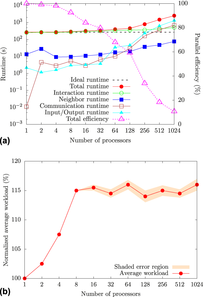
(a) Runtime breakdown of all components and parallel efficiency and (b) normalized average workload with respect to the serial CAC simulation in weak scaling, with 492 elements per processor. In (b), the shaded error region represents the standard deviation of the workload of all processors.

In strong scaling, four simulation cells, with the number of 2NN elements being 3430, 29,660, 102,690, and 246,520, respectively, are used. With a uniform element size of 2197 atoms and a lattice constant of 3.52 Å, the largest simulation cell has a size of 182.6 × 182.6 × 182.6 nm. As a result, the smallest and the largest simulation cells correspond to equivalent full atomistic models containing about 7.5 million and about 541.6 million atoms, respectively. Traction-free boundary conditions and {100} crystallographic orientations are applied along the three directions, with the EAM potentialReference Mishin, Farkas, Mehl and Papaconstantopoulos72 describing the interatomic interactions. Instead of building the simulation cell from scratch, the CAC simulator the system configuration from pre-existing restart files. It followed that a dynamic run with the velocity Verlet algorithm was performed under an NVE ensemble. We remark that the results presented here are representative of dynamic runs using other options (qd and ld) because all of them adopt similar equations of motion. With a time step of 2 fs, each run consists of 200 steps, with 1 input, 1 neighbor establishment, 2 neighbor updates, and 2 outputs.
For all simulation cells, when the number of processors is relatively small (<64 and <256 for the smallest and the largest simulation cells, respectively), the interaction and neighbor steps are shown to be the most CPU-intensive operations, with no major bottleneck caused by data input/output, similar to atomistic simulations. In all cases, when more than 1 processor is used, the interprocessor communication time is almost invariant with the number of processors. However, the runtime spent on input/ouput increases rapidly as the number of processors grows; it should be noted that the results may change significantly if different frequencies for output and neighbor updates are used. In addition, because of the shared elements, the total memory usage is no longer invariant but increases as more processors are used [Fig. 6(f)]. As expected, both parallel scalability and memory usage improve as the simulation cell size increases, as shown in Figs. 6(e) and 6(f).
In weak scaling, the number of processors in one simulation varies from 1 to 1024, with about 492 elements per processor. As a result, the largest simulation cell has a size of 231.9 × 231.9 × 231.9 nm, with 503,808 elements, corresponding to 1,106,866,176 interpolated atoms, which is more than double the previous largest EAM-based CAC models that contained about 552.7 million atoms.Reference Xiong, Rigelesaiyin, Chen, Xu, McDowell and Chen16 Other simulation settings are the same as those in strong scaling. It is found that the runtime spent on data loading can be negligible compared to the very long runtime of the CAC simulation on small or medium number of processors. Nonetheless, as the number of processors increases, the runtime for interprocessor communication and input/output increases much more quickly than that for interatomic interactions and establishing/updating neighbors, as shown in Fig. 7(a). In particular, with 1024 processors, the runtime for input/output, which is not fully parallelized as discussed in Sec. IV.A, constitutes more than half the total runtime; in other words, the input/output procedure may become a new bottleneck for achieving high parallel scalability according to Amdahl’s law.Reference Amdahl73 In this regard, we will conduct further investigation to improve the parallel scalability of the CAC simulator as part of our future work. We remark that the processor workload is well balanced, as shown in Fig. 7(b).
V. PyCAC SOFTWARE
In this section, we present the features, the Python scripting interface as well as the compilation and execution of the PyCAC software. More specific details of PyCAC, including the input script format and some example problems, can be found at www.pycac.org.
A. Features
The PyCAC code can simulate monatomic pure FCC and pure BCC metals using the LJ and EAM interatomic potentials in conservative systems. In the coarse-grained domain, 3D trilinear rhombohedral elements are used to accommodate dislocations in 9 out of 12 sets of {111}〈110〉 slip systems in an FCC lattice as well as 6 out of 12 sets of {110}〈111〉 slip systems in a BCC lattice, as shown in Figs. 3(c) and 3(d).
We remark that there is no theoretical challenge in extending the current PyCAC code to admit more slip systems, crystal structures, interatomic potentials, element types, and materials. In fact, AFT was originally designed with polyatomic crystalline materials in mind,Reference Chen and Lee74,Reference Chen and Lee75 and CAC has been applied to a 1D polyatomic crystal with trilinearReference Xiong, Chen, Zhang, McDowell and Chen76 and nonlinear shape functions,Reference Chen, Diaz, Xiong, McDowell and Chen36 an ideal brittle FCC crystal with 2D triangular elementsReference Deng, Xiong and Chen38 or with 3D tetrahedral and 3D pyramid elements,Reference Deng and Chen39 silicon using the SW potential,Reference Xiong, McDowell and Chen43 a 2D Cu single crystal with 2D quadrilateral elements,Reference Xiong, Rigelesaiyin, Chen, Xu, McDowell and Chen16 2D FCC Cu single crystalReference Chen, Xiong, McDowell and Chen47 and polycrystalReference Chen, Li, Xiong, Li, Yang, Zheng, McDowell and Chen48 with 2D quadrilateral elements, and 2D superlattices with 2D quadrilateral elementsReference Chen, Li, Diaz, Li, Chen and McDowell49 as well as strontium titanate using a rigid-ion potential with 3D cubic elements.Reference Yang, Xiong, Deng and Chen42,Reference Yang, Zhang and Chen44,Reference Yang and Chen45 These simulations were conducted using other versions of CAC.
B. Python scripting interface
In PyCAC, the Python scripting interface is a Python wrapper module for CAC’s underlying Fortran 2008 code, allowing handling of the program’s input and output as well as links to some external visualization software. Written in Python 3 and contained in pycac.py, the Python module provides a robust user interface to facilitate parametric studies via CAC simulations without interacting with the Fortran code and to improve handling of input, output, and visualization options, as illustrated in Fig. 8. Mainly working on local computers, the Python module serves as an interface with high performance computing clusters. In particular, the module consists of three main components:
(i) input.py() for generation and manipulation of CAC simulation cells on local computer via a graphical user interface, as well as submitting jobs via job schedulers on high performance computing clusters, e.g., those on NSF XSEDE.Reference Towns, Cockerill, Dahan, Foster, Gaither, Grimshaw, Hazlewood, Lathrop, Lifka, Peterson, Roskies, Scott and Wilkins-Diehr71 A CAC simulation requires at least two types of files as input: an input script and the analytic or tabulated interatomic potential files. If the users intend to continue a previous run, a restart file with previously saved system configuration needs to be provided as well. Note that some or all elements from a previous run can be refined into atomic scale upon reading the restart file. This is useful, for example, to correctly simulate the migration of a dislocation whose pathway is not aligned with the interelemental gap.Reference Xu, Xiong, Deng and McDowell15
(ii) output.py() for downloading the CAC simulation output data from clusters before processing them locally. A CAC simulation outputs three main types of files: (i) vtk files in the legacy ASCII format containing elemental, nodal, and atomic information (positions, energies, forces, stresses, etc.); (ii) restart files containing system configuration information; and (iii) a log file recording relevant lumped simulation data, e.g., system force/energy and number of elements/atoms, during a run. It follows that the output.py() component reads the vtk files and interpolates all atoms inside the elements in the coarse-grained domain. These interpolated atoms, together with the real atoms in the atomistic domain (also read from the vtk files), are used to generate LAMMPS dump files that can be visualized by atomistic model viewers and/or read by LAMMPS directly to carry out equivalent fully-resolved atomistic simulations. CAC simulation results may also be processed via the data analyzer which will be presented in the near future.
(iii) visualization.py() for integrating some visualization software. Currently, the dump files and vtk files are visualized by OVITOReference Stukowski58 and ParaView,Reference Schroeder, Martin and Lorensen63 respectively, as discussed in Sec. III.D.
Python scripting interface scheme. First, input.py() creates CAC simulation cells via a graphical user interface on a local computer and submits jobs via job schedulers on high performance computing clusters; then CAC simulations compiled from the underlying Fortran code are run following Figs. 1 or 5; once the simulations finish, output.py() downloads the output data from clusters before processing them locally using the data analyzer; in the end, visualization.py() employs some visualization software to render CAC simulation results.

C. Compilation and Execution
In PyCAC, the CAC algorithm is implemented in Fortran 2008 and parallelized with MPI-3, wrapped by a Python scripting interface written in Python 3. Therefore, the PyCAC code can be compiled with any MPI, Fortran, and Python compilers that support MPI-3, Fortran 2008, and Python 3, respectively. For example, the parallel scalability benchmark simulations in Figs. 6 and 7 were run using an executable compiled by Intel Fortran compiler version 17.0 wrapped by MVAPICH2 version 2.3.
Potential users may explore PyCAC by running simulations via the MATerials Innovation Network (MATIN, https://matin.gatech.edu),Reference Kalidindi, Brough, Li, Cecen, Blekh, Congo and Campbell77 a cloud-based e-collaboration platform for accelerating materials innovation developed at the Georgia Institute of Technology (GT) with support of the GT Institute for Materials. While MATIN is focused on emergent field of materials data science and informatics, it offers a comprehensive range of functionality targeting the materials science and engineering domain. After signing up for a free account, a user can run the PyCAC code via MATIN on GT’s Partnership for an Advanced Computing Environment (PACE) cluster or on NSF XSEDE.Footnote a
VI. CONCLUSIONS
In this work, we present a novel implementation of the CAC method—PyCAC—an efficient, user-friendly, and extensible CAC simulation environment which is implemented mainly in Fortran 2008 and wrapped with a Python scripting interface. First, the theoretical background of the CAC method was briefly reviewed. Then, the serial algorithms of dynamic, quasistatic, and hybrid CAC, along with some programming techniques used in the PyCAC code were discussed. In addition, the parallel algorithm/scalability of the CAC simulator and some specific details of the PyCAC software were presented. Additional information of PyCAC can be found at www.pycac.org.
While the CAC method has a high coarse-graining efficiencyReference Xu, Che, Xiong, Chen and McDowell8 and the PyCAC software shows good scaling performance, there is still room for improvement in the code performance by parallelizing the input/output. Future development of code features will involve implementation of more types of finite elements and interatomic potentials to accommodate more crystalline materials such as multicomponent and polyatomic materials. New types of finite elements will also be used to replace the filled-in atoms at the otherwise zigzag simulation cell boundaries to reduce the computational cost, particularly in the case of PBCs. Other versions of the CAC simulator, e.g., the one in Ref. 78, may be incorporated into PyCAC. Future extensions also include developing adaptive mesh refinement schemes for dislocation migration, in which case the evaluation point density may evolve with time, requiring more complicated algorithms to dynamically re-balance the processor workload.
Supplementary Material
To view supplementary material for this article, please visit https://doi.org/10.1557/jmr.2018.8.
ACKNOWLEDGMENTS
These results are based upon work supported by the National Science Foundation as a collaborative effort between Georgia Tech (CMMI-1232878) and University of Florida (CMMI-1233113). Any opinions, findings, and conclusions or recommendations expressed in this material are those of the authors and do not necessarily reflect the views of the National Science Foundation. The authors thank Dr. Jinghong Fan, Dr. Qian Deng, Dr. Shengfeng Yang, Dr. Xiang Chen, Mr. Rui Che, Mr. Weixuan Li, and Mr. Ji Rigelesaiyin for helpful discussions, and Dr. Aleksandr Blekh for arranging execution of PyCAC via MATIN. The work of SX was supported in part by Georgia Tech Institute for Materials and in part by the Elings Prize Fellowship in Science offered by the California NanoSystems Institute (CNSI) on the UC Santa Barbara campus. SX also acknowledges support from the Center for Scientific Computing from the CNSI, MRL: an NSF MRSEC (DMR-1121053). LX acknowledges the support from the Department of Energy, Office of Basic Energy Sciences under Award Number DE-SC0006539. The work of LX was also supported in part by the National Science Foundation under Award Number CMMI-1536925. DLM is grateful for the additional support of the Carter N. Paden, Jr. Distinguished Chair in Metals Processing. This work used the Extreme Science and Engineering Discovery Environment (XSEDE), which is supported by National Science Foundation grant number ACI-1053575.