





Impact statement
This article introduces a dual framework combining data assimilation (DA) and machine learning (ML) to enhance flow prediction in configurations exhibiting periodic temporal properties due to oscillatory motion of immersed bodies. This goes a step ahead of classical studies that rely on data-driven techniques for simplified arrangements that impose highly restrictive temporal constraints. Here, we propose a sliding-window strategy that leverages the accurate, time-resolved estimates provided by the DA technique to train specialized ML models tailored to specific flow conditions. This paves the way for the construction of a future gating model that can adaptively weight each specialized model to maximize accuracy. The approach offers a scalable path toward robust flow prediction in more complex and diverse configurations.
1. Introduction
Over the past decade, methods based on data usage (data-driven, data-informed, data-aware…) have provided advancement on a wide range of problems in computational and experimental fluid mechanics. Such approaches have been used to develop equation-free or partially learned flow representations through reduced-order modeling (Kutz, Reference Kutz, Falcone and Rozza2023) and system identification techniques (Brunton et al., Reference Brunton, Proctor and Kutz2016), to design and optimize estimation and control strategies in unsteady flows (Noack et al., Reference Noack, Morzynski and Tadmor2011; Brunton and Noack, Reference Brunton and Noack2015), and to improve or complement classical closure models in both Reynolds-averaged Navier–Stokes (RANS) and Large Eddy Simulations turbulence frameworks (Pope, Reference Pope2000; Duraisamy et al., Reference Duraisamy, Iaccarino and Xiao2019). These strategies include methods that extract information from limited measurements (sparse sensing), reconstruct flow fields, learn model relationships through supervised training, and adaptively correct predictions in real time, and share the common goal of exploiting high-fidelity or experimental data to enhance predictive capability, stability, or computational efficiency across diverse flow regimes.
Within these data-driven approaches, measurements, commonly referred to as sensors, play a central role. In Data Assimilation (DA) (Asch et al., Reference Asch, Bocquet and Nodet2016; Evensen et al., Reference Evensen, Vossepoel and van Leeuwen2022), sensor information, also known as observations, is continuously integrated into the numerical model to correct the evolving flow state (Mons et al., Reference Mons, Chassaing, Gómez and Sagaut2016; Villanueva et al., Reference Villanueva, Truffin and Meldi2024a; Reference Villanueva, Truffin, Borée and Meldi2025; Jeanney et al., Reference Jeanney, Hetherington, Ahmed, Lanceta, Saiz, Perez and Le Clainche2025) and, in some formulations, to adjust unknown spatially distributed physical model parameters (Franceschini et al., Reference Franceschini, Sipp and Marquet2020; Ben Ali et al., Reference Ben Ali, Tissot, Aguinaga, Heitz and Mémin2022; Moussie et al., Reference Moussie, Errante and Meldi2024). Machine learning (ML) methods (Brunton et al., Reference Brunton, Noack and Koumoutsakos2020) typically use sensor data offline to train models that identify patterns and extract flow features (Strofer et al., Reference Strofer, Wu, Xiao and Paterson2018), super-resolution reconstruction (Fukami et al., Reference Fukami, Fukagata and Taira2019), or emulate governing equations (Raissi et al., Reference Raissi, Perdikaris and Karniadakis2019). While both paradigms rely on the quality and representativeness of sensor information, their effectiveness in both cases strongly depends on how well the available data captures the relevant flow dynamics.
Rather than viewing DA and ML as competing approaches, recent perspectives emphasize their complementarity and the potential for unified frameworks that combine their respective strengths (Geer, Reference Geer2021). However, several key challenges emerge when extending these data-driven techniques beyond idealized conditions. Most current studies evaluating DA and ML frameworks in numerical fluid simulations still focus on simplified configurations, often assuming statistically stationary regimes (Zhang et al., Reference Zhang, Xiao, Luo and He2022), employing low-dimensional toy models (Bocquet et al., Reference Bocquet, Brajard, Carrassi and Bertino2019; Brajard et al., Reference Brajard, Carrassi and BocquetMand Bertino2020; Malartic et al., Reference Malartic, Farchi and Bocquet2022; Özalp et al., Reference Özalp, Nóvoa and Magri2026), or constructing manifolds of reduced-order models (Nóvoa and Magri, Reference Nóvoa and Magri2025). Although these settings provide valuable insight into methodological performance, additional developments are required to address real-world applications, which typically involve moving bodies with complex geometries, multiscale interactions, and strongly time-dependent phenomena. In such scenarios, additional complexities arise, including:
-
(i) Sensors might be moving, or the relative distance between the sensors and the regions of physical interest (such as surfaces for integral evaluations, wake structures, or detachment zones) can vary with time, as in the case of moving bodies. For example, in the study of oscillating or pitching airfoils, the instantaneous positions of pressure sensors mounted on the surface or in the wake change continuously with respect to the characteristic flow features (Piccolo Serafim et al., Reference Piccolo Serafim, Cervi, Smalley, Kramer, Huang and Dowell2025). This relative motion modifies the local sampling of flow quantities and complicates both state estimation (or field reconstruction) and model training, particularly when the flow exhibits large variations in separation and reattachment over a cycle.
-
(ii) Beyond sensor-related issues, unsteady configurations often involve complex interactions across spatial and temporal scales, such as vortex shedding influencing upstream boundary-layer development or unsteady separation affecting distant wake regions. These nonlocal and phase-dependent couplings evolve during the motion cycle and cannot be captured by purely local measurements or static mappings. For DA, this complicates the propagation of observational information across the domain, whereas for ML, it challenges the construction of models that remain valid as these long-range dependencies shift over time. Accounting for such dynamic multiscale interactions requires assimilation and learning strategies capable of representing nonlocality and capturing correlations that change with the instantaneous flow state.
-
(iii) Local extreme events might occur, leading to external intermittency, time-varying statistics, and the necessity for streaming data-processing methodologies. These factors also highlight the limitations of offline-trained ML models, which may fail to predict high-intensity perturbations or transient phenomena absent from the original training dataset. As the underlying dynamics evolve, previously learned dependencies may become less relevant, and new correlations can emerge on shorter time scales. Capturing these instantaneous and evolving relationships requires online adaptation mechanisms that can integrate new information as it becomes available.
To analyze the challenges previously listed, window-based strategies provide a natural framework for maintaining model relevance in nonstationary flow configurations. In the present work, we aim to employ the augmented information estimated by a sequential DA technique, namely an Ensemble Kalman Filter (EnKF) combining state estimation with parameter optimization (Evensen, Reference Evensen2009), to train multiple black-box models using the random forest regression (RFR) algorithm (Breiman, Reference Breiman2001), within a sliding-window framework. The test case considered involves a flow with periodic behavior, allowing each window to focus on locally coherent dynamics within the oscillation cycle. In this sense, the windowing strategy can provide a foundation for a temporal mixture of experts (MoE) framework, with different regressors specializing in distinct phases of the motion, akin to spatial MoE approaches previously explored in complex or multiregion flows (Yuksel et al., Reference Yuksel, Wilson and Gader2012). This configuration shares conceptual similarities with previous variational DA studies of rotating cylinders in laminar regimes (Mons et al., Reference Mons, Chassaing and Sagaut2017), which likewise aimed to couple physical models with assimilation strategies to improve flow reconstruction and control. However, to the best of our knowledge, no prior work has applied DA or ML to configurations involving extended body motion, which modifies the near-wake dynamics and introduces greater temporal variability.
This investigation extends previous studies coupling DA and ML by Valero and Meldi (Reference Valero and Meldi2025a), where it was observed that state estimation and a local parameter optimization via EnKF could enhance the near-wall resolution of wall-bounded turbulent flows with an under-refined mesh, achieving accuracy comparable to that of high-fidelity simulations. It was also observed that flow snapshots produced by state estimation can be used to train an RFR algorithm that mimics the DA flow updates. This ML-based flow correction yields improved computational efficiency compared to the DA approach (Valero and Meldi, Reference Valero and Meldi2025b), which can be particularly costly in ensemble-based or adjoint formulations. However, the analyses were conducted under specific conditions, which are particular features of the test case investigated, namely:
-
• The flow statistics were steady with time, so that the same physical behavior was represented throughout the assimilation period (observation window). Furthermore, spatial inhomogeneity was solely restricted to the wall-normal direction, resulting in all grid layers equidistant from the immersed walls experiencing identical flow physics.
-
• No-slip boundary conditions were imposed at the walls. This eliminated the influence of time-dependent wall motion, which would otherwise arise in cases involving immersed moving bodies.
In the current work, this framework is extended to the analysis of a moving immersed body in an oscillatory regime, where the flow exhibits a wide variety of dynamical features that vary both with the phase of the oscillatory cycle and locally within the computational domain, and where the solid body undergoes time-dependent motion. Although the flow exhibits locally repeatable, phase-aligned behavior across cycles, this combination of global nonstationarity and phase-dependent coherence introduces an additional layer of complexity beyond that previously explored. Besides, this phase-dependent behavior motivates the use of a sliding-window strategy, in which each window captures a locally coherent phase of the oscillation.
Within this scope, the article is structured as follows. Section 2 describes the numerical ingredients and methodologies employed. The test case used for the analyses is introduced in Section 3. Strategies aimed at enhancing predictive capabilities through DA and ML are then presented in Sections 4 and 5, respectively. Finally, conclusions and perspectives are discussed in Section 6.
2. Numerical ingredients
2.1. Numerical solver and immersed boundary method
The Navier–Stokes equations for incompressible flows applied to Newtonian fluids and negligible temperature gradients can be written as (2.1)–(2.2), with (2.2) expressed in vector notation:


where
$ \boldsymbol{u} $
 is the velocity,
$ t $
 is the time,
$ \nu $
 is the kinematic viscosity, and
$ p=P/\rho $
 is the normalized pressure field
$ P $
 with respect to density
$ \rho $
 . In low-Reynolds-number regimes, the flow can exhibit two-dimensional features, as observed in the present investigation. The flow is analyzed in a plane where
$ z= constant $
 . Therefore, the position vector is
$ \boldsymbol{x}=\left(x,y\right) $
 in Cartesian coordinates where
$ x $
 and
$ y $
 are the streamwise and crosswise positions, respectively. The velocity field is represented as
$ \boldsymbol{u}=\left({u}_x,{u}_y\right) $
 . One can include an additional source term to account for body forces such as gravity, centrifugal, Coriolis, or electromagnetic contributions. In the present analysis,
$ {\boldsymbol{f}}_P $
 represents a penalization term for a classical immersed boundary method (IBM).
$ {\boldsymbol{f}}_P $
 accounts for the presence of immersed rigid solid obstacles, whose bodies are located in a region
$ {\Omega}_b $
 . Angot et al. (Reference Angot, Bruneau and Fabrie1999) showed by means of asymptotic analysis that the solution of the velocity field with this source term converges to the standard incompressible Navier–Stokes equations with a Dirichlet boundary condition at the immersed boundary for the velocity. The penalization term is then defined as

Here,
$ {\boldsymbol{u}}_{\boldsymbol{ib}} $
 is the target velocity for the solid obstacle, and
$ {\Omega}_f $
 is the region of the domain accessible to the fluid.
$ {\alpha}_p $
 is a penalization time-step parameter, which depends on the time step
$ \Delta t $
 employed during discretization, and is commonly defined for
$ {\alpha}_p\in \left[0,1\right] $
 , where lower values increase accuracy but are more prone to numerical instabilities (Kadoch et al., Reference Kadoch, Kolomenskiy, Angot and Schneider2012). Here, all case studies are numerically investigated using customized solvers developed within the open-source framework (OpenFOAM - Field Operation And Manipulation, 2021), which employs a finite-volume discretization of equations (2.1)–(2.2). Time advancement is performed using the PISO scheme (Issa, Reference Issa1986) and a second-order backward scheme. Second-order centered schemes handle spatial discretization. The customized solver has been specifically designed for the study of cylinder-based geometries with IBMs and has been previously validated and employed in related works (Er and Meldi, Reference Er and Meldi2025).
2.2. Data assimilation: Ensemble Kalman Filter for state estimation and parameter optimization
The EnKF (Evensen, Reference Evensen1994) is a Monte Carlo extension of the classical Kalman Filter (KF) (Kalman, Reference Kalman1960). It propagates over time both the physical system state
$ \boldsymbol{u} $
 (commonly the velocity field discretized over the computational domain in CFD applications) and its associated uncertainty, represented by the error covariance matrix
$ \boldsymbol{P}=\unicode{x1D53C}\left[\left(\boldsymbol{u}-{\boldsymbol{u}}^t\right){\left(\boldsymbol{u}-{\boldsymbol{u}}^t\right)}^T\right] $
 , where
$ {\boldsymbol{u}}^t $
 denotes the (unknown) true state. To avoid explicitly defining the high-dimensional matrix
$ \boldsymbol{P}\in {\unicode{x211D}}^{n_{DF}\times {n}_{DF}} $
 , with
$ {n}_{DF} $
 denoting the number of degrees of freedom (e.g., twice the number of mesh elements in two-dimensional CFD configurations), the EnKF represents the state as an ensemble of realizations, referred to as ensemble members, each with a distinct state vector
$ {\boldsymbol{u}}_i $
 (
$ i\in \left[1,{N}_e\right] $
 , where
$ {N}_e<<{n}_{DF} $
 is the number of ensemble members). The ensemble mean
$ \overline{\boldsymbol{u}} $
 approximates the true state
$ {\boldsymbol{u}}^t $
 , while the deviations of each member from the mean are collected in the anomaly matrix
$ \boldsymbol{X} $
 , defined as


If the ensemble is significantly large to represent the system statistics and its members are statistically independent, the error covariance matrix
$ \boldsymbol{P} $
 can then be efficiently approximated as

where
$ \boldsymbol{X}\in {\unicode{x211D}}^{n_{DF}\times {N}_e} $
 . The EnKF follows a two-step cycle. The first step, referred to as forecast, and represented by (
$ {\cdot}^f $
 ), advances each ensemble member from time
$ k-1 $
 to
$ k $
 through a numerical model
$ \mathcal{M}\left(\theta, \boldsymbol{u}\right) $
 , which denotes the discrete representation of the underlying physical model governed by the parameters
$ \theta $
 :

If observational data is available at time k, an analysis step follows, represented by (
$ {\cdot}^a $
 ), where the ensemble is updated to optimally combine the model forecast and the measurements, minimizing the posterior error covariance matrix
$ {\boldsymbol{P}}_k^a $
 . An extended-state formulation (Evensen, Reference Evensen2009) can also be employed, in which selected model parameters
$ \theta $
 are estimated jointly with the state, leading to a reduction in the model bias and yielding an augmented state vector
$ {\boldsymbol{u}}^{\prime }={\left[\boldsymbol{u},\theta \right]}^T $
 .
To maintain dimensional consistency in the EnKF formulation, an ensemble of
$ {N}_e $
 observation vectors is required. These are assembled into the observation matrix
$ {\boldsymbol{Y}}_k\in {\unicode{x211D}}^{n_o\times {N}_e} $
 . However, applying the same observation vector to all ensemble members causes the ensemble-based posterior covariance to be systematically underestimated. Two main approaches exist to address this issue. The first is deterministic and relies on square-root formulations of the EnKF to ensure that the ensemble maintains the right covariance structure during the update process (Tippett et al., Reference Tippett, Anderson, Bishop, Hamill and Whitaker2003). The second one is stochastic and consists of introducing random perturbations in the observations, which is essential for ensuring that measurements are properly treated as random variables and for preventing an underestimation of the updated state variance (Burgers et al., Reference Burgers, van Leeuwen and Evensen1998). The latter is the approach adopted in the present work, in which we provide a suitable perturbation of the observation vector
$ {\boldsymbol{y}}_k\in {\unicode{x211D}}^{n_o\times 1} $
 . Each perturbation is modeled as Gaussian noise
$ {\boldsymbol{e}}_i $
 with zero mean and covariance
$ {\boldsymbol{R}}_k\in {\unicode{x211D}}^{n_o\times {n}_o} $
 , which represents the observation uncertainty. The matrix
$ {\boldsymbol{R}}_k $
 is typically assumed diagonal, implying that the measurement errors are Gaussian, unbiased, and mutually independent. In the limit of an infinitely large ensemble,
$ {\lim}_{N_e\to +\infty}\unicode{x1D53C}\left[\left(\boldsymbol{e}-\unicode{x1D53C}\left[\boldsymbol{e}\right]\right){\left(\boldsymbol{e}-\unicode{x1D53C}\left[\boldsymbol{e}\right]\right)}^T\right]=\boldsymbol{R} $
 , which becomes time-independent. Thus, each ensemble realization of the observation matrix can be expressed as
$ {\left[{\boldsymbol{Y}}_k\right]}_i={\boldsymbol{y}}_k+{\boldsymbol{e}}_i $
 , where
$ {\boldsymbol{e}}_i\sim \mathcal{N}\left(0,\boldsymbol{R}\right) $
 .
The EnKF also requires a sampling operator
$ \mathcal{H}\left({\boldsymbol{u}}_k^f\right) $
 , where
$ \mathcal{H} $
 serves as an interpolation operator that maps the forecasted system state from the model space onto the observation space. Analogous to the anomaly matrix with the forecasted system state
$ {\boldsymbol{X}}^f $
 following (2.5), this projected ensemble is represented by the matrix
$ {\boldsymbol{S}}_k^f $
 , whose columns correspond to normalized anomalies of the sampled states. These are computed from the ensemble mean
$ \overline{\mathcal{H}\left({\boldsymbol{u}}_k^f\right)} $
 as:


The Kalman gain matrix
$ {\boldsymbol{K}}_k $
 providing the most optimal weight between the state and the observations can be expressed as in (2.10) (Carrassi et al., Reference Carrassi, Bocquet, Bertino and Evensen2018):

All the elements described above are required to calculate the updated system’s state
$ {\boldsymbol{u}}_k^a $
 and model parameters
$ {\theta}_k^a $
 as in (2.11), which are subsequently used to advance the numerical model
$ \mathcal{M}\left({\theta}_{i,k+1:k},{\boldsymbol{u}}_{i,k}\right) $
 during the next iteration at time step
$ k+1 $
 . Figure 1 shows a schematic of the two-step procedure.

Ensemble Kalman Filter algorithm, highlighting the forecast and analysis steps (adapted from Valero (Reference Valero2025)).

Figure 1. Long description
The graph uses a horizontal axis labeled K, which corresponds to the DA cycles and a vertical axis with two labels u and y. The first represents the state of the system while the second denotes some observations. A dashed light blue line at the top represents the Truth.
At cycle k sub 0, a blue oval labeled usub 0 super a contains an ensemble of points that represent the prior state.
Moving to cycle k sub 1, orange dashed lines represent the Forecast step, which is the time evolution the dynamical physical model, leading from k sub 0 to a green oval labeled u sub 1 super f. A vertical red arrow points upward from this green oval to a red oval labeled u sub 1 super a, representing the Analysis step. Above this, a purple oval contains a triangle labeled y sub 1, representing the Observation. One can notice that the analysis step is a “correction” step, in which the prevision made by the model is adjusted to account for the presence of some sparse measurements or “observations” at the same time step.
At cycle k sub 2, the process repeats. Orange dashed lines lead to a green oval u sub 2 super f. Above it is a red oval u sub 2 super a, and at the top is a purple observation oval y sub 2.
At cycle k sub 3, the ensemble in the green oval u sub 3 super f is closer to the Truth line. The red analysis oval u sub 3 super a and the purple observation oval y sub 3 are positioned at the highest point of the cycle, nearly intersecting the Truth line. The procedure converges after several analysis steps toward a solution for the model that complies with the uncertainty prescribed to the observation.
The EnKF is selected for the present analysis thanks to its capacity to operate with nonlinear model forecasts with moderate computational resources. The usage of more complex strategies, such as particle filters (van Leeuwen et al., Reference van Leeuwen, Künsch, Nerger, Potthast and Reich2019), would dramatically increase the computational costs, therefore precluding the possibility of performing extended sensitivity analyses such as the ones reported in the present work.
2.3. Random forest regression
RFR (Breiman, Reference Breiman2001) is an ensemble learning algorithm that builds a number of
$ N $
 decision trees during the training phase. The final output is estimated as the average of the decision tree predictions, thereby enhancing accuracy and robustness, and making it a reliable model for regression tasks. By combining bootstrapping and random feature selection to account for each decision tree’s predictions, it reduces overfitting risk and enhances model stability. Each decision tree
$ n\in \left[1,\dots, N\right] $
 is constructed using a subset of the entire training dataset
$ {m}_T $
 and selects splitting criteria or nodes to progress in tree depth. Commonly, the splitting criterion aims to minimize the variance of the target variable within the resulting subsets; that is, the split point is chosen to minimize the mean square error (MSE) of the child nodes (MSEchild) and to maximize the reduction in MSE (
$ \Delta \mathrm{MSE} $
 ) from the parent to the child nodes, which is computed as the difference between the MSE in the parent node and the weighted sum of the MSEs in the resulting child nodes. These quantities are calculated using the following expressions:


where
$ m $
 represents the number of samples of the parent node,
$ {\mathcal{Y}}_j $
 and
$ {\hat{\mathcal{Y}}}_j $
 point out to the actual and predicted target value for the sample
$ j\in \left[1,m\right] $
 , and
$ {m}_{\mathrm{left}} $
 and
$ {m}_{\mathrm{right}} $
 are associated with the number of samples in the left and right child nodes. The MSEs for the parent, left child, and right child nodes are
$ {\mathrm{MSE}}_{\mathrm{parent}} $
 ,
$ {\mathrm{MSE}}_{\mathrm{left}} $
 , and
$ {\mathrm{MSE}}_{\mathrm{right}} $
 , respectively.
At each parent node, the dataset is divided into two subsets based on a specific feature
$ {\mathcal{X}}_l $
 and a split point, yielding two child nodes. Here, each row of the input matrix corresponds to a training point, and each column to a feature. The left child node usually represents data meeting the split criteria (e.g., feature value
$ {\mathcal{X}}_{j,l}\le $
 split point), while the right child node does not (e.g., feature value
$ {\mathcal{X}}_{j,l}> $
 split point). This splitting-nodes procedure continues recursively for each child node until predefined stopping criteria are met, which, in our case, is the minimum number of samples required to form a leaf node. In the present work, some local resolved flow quantities in the solid region
$ {\Omega}_b $
 improved by means of the DA technique serve as the features
$ {\mathcal{X}}_l $
 of the algorithm, while the predicted target
$ \hat{\mathcal{Y}} $
 is the IBM penalty forcing term
$ {\hat{\boldsymbol{f}}}_P $
 (the details are provided in Section 5). This source term is defined by a set of local parameters representing
$ {\alpha}_p $
 . Therefore, we refer to the architecture with the operator
$ {\mathcal{F}}_{\mathrm{p}.\mathrm{o}.} $
 , where “p.o.” stands for parameter optimization, since the black-box algorithm learns the parameter corrections estimated by the EnKF. A scheme summarizing the main concepts related to RFR is shown in Figure 2.
Scheme of random forest regression.

Figure 2. Long description
At the top, a rectangular box contains many colored circles representing the total number of samples m sub T. A color scale bar to the right ranges from blue to red. Three overlapping shaded regions within the sample box point down to multiple separate decision trees.
Each decision tree starts with a parent node containing m samples and a M S E sub parent value. From the parent node, two arrows branch out based on a split point condition: x sub j, l less than or equal to split point on the left, and x sub j, l greater than split point on the right. These lead to a left child node with m sub left samples and M S E sub left, and a right child node with m sub right samples and M S E sub right.
The trees are labeled DECISION TREE 1 with output y-hat sub j, 1, DECISION TREE 2 with output y-hat sub j, 2, up to DECISION TREE N with output y-hat sub j, N. An ellipsis indicates additional trees in between.
On the far left, a long vertical arrow points downward, labeled with F sub p.o. and f-hat sub P, accompanied by text indicating that the decision trees aim to predict the local resolved quantities in the solid region Omega sub b enhanced by D A.
At the very bottom, the final output is defined by the equation: y-hat sub j equals the summation from n equals 1 to N of y-hat sub j, n.
Alternative regressors, such as neural networks (NNs) or Gaussian Process (GP) models, could in principle be considered for this study. RFR, however, offers several practical advantages. Compared to NNs, RFR requires minimal input preprocessing, is more interpretable, and typically exhibits strong robustness against overfitting, particularly for tabular regression problems (Wang et al., Reference Wang, Wu and Xiao2017; Roßbach, Reference Roßbach2018). For the latter, while GPs can provide both predictive means and uncertainties and often achieve high accuracy in small-data regimes (Bajer et al., Reference Bajer, Pitra and Holeňa2015; Mlakar et al., Reference Mlakar, Tušar and Filipic2019), their standard formulation requires constructing and factorizing a dense kernel (covariance) matrix
$ \mathcal{K}\in {\unicode{x211D}}^{m_T\times {m}_T} $
 , which encodes the pairwise statistical relationships between all training points
$ {\mathcal{X}}_j $
 . For large datasets, as considered here (
$ {m}_T\approx {10}^6 $
 samples per model, see Section 5), the memory cost
$ \mathcal{O}\left({m}_T^2\right) $
 and computational cost of factorization
$ \mathcal{O}\left({m}_T^3\right) $
 make exact GP regression infeasible. By contrast, RFR scales efficiently to millions of samples, making it a computationally convenient and robust choice for the present work.
2.4. Sliding windows and their role with data assimilation and machine learning
Both DA and hybrid ML are data-driven techniques that blend a physical model and observations of the same physical phenomenon to improve predictive accuracy. However, they employ different strategies to achieve it. For the former, sparse observations in time and space are combined with the governing equations to accurately predict the system state with the highest level of precision. In contrast, for the latter, some black-box models trained with a large, densely sampled set of data typically replace or correct some of the terms of the governing equations that do not offer globally accurate predictive capabilities (e.g., Reynolds stress tensor or subgrid-scale model) (Kutz, Reference Kutz2017; Beck et al., Reference Beck, Flad and Munz2019), or that are computationally expensive to solve (e.g., Poisson equation) (Weymouth, Reference Weymouth2022). Despite these differences, both approaches must contend with the fact that the underlying flow physics can vary significantly over time, meaning that the information content of the observations and the appropriate modeling strategy may change throughout the simulation period, motivating the use of smaller windows that better capture the local flow dynamics.
In view of these circumstances, within the DA field, interest in dividing the full observation window into a sequence of smaller, consecutive (and, optionally, overlapping) sub-windows arises for several reasons. First, in the case of variational approaches, each sub-window—referred to in this context as assimilation windows—can focus on a narrower temporal frame over which model error growth remains controlled, thereby simplifying the modeling and assimilation task. Chandramouli et al. (Reference Chandramouli, Memin and Heitz2020) and Wang and Zaki (Reference Wang and Zaki2025) argued that, in turbulent flows, the assimilation window used in 4DVar formulations must be shorter than the Lyapunov timescale to ensure that the physical model remains close to the truth over each window and that the adjoint gradients remain well-conditioned. Sliding windows have also been employed in the context of statistical DA methods, such as particle filters, which are well-suited to handle nonlinear and non-Gaussian uncertainties. Albarakati et al. (Reference Albarakati, Bušidić and Van Vleck2024) introduced a Proper Orthogonal Decomposition-based reduced-order framework in which the projection operator is recomputed using a sliding subset of snapshots (i.e., sliding windows), allowing the reduced basis to adapt dynamically to changes in the system by extracting the dominant spatiotemporal modes governing the observed data.
Additionally, analogous ideas arise in how these methods manage the temporal frequency of assimilation, that is, the time interval between successive assimilation steps. Meldi (Reference Meldi2018) studied the effect of the frequency of time sampling of observations on the accuracy of the prediction by the assimilation operator, which depends on the characteristic average advection time. In addition, the concept of sliding windows can be highly relevant to non-sequential statistical approaches, such as the Ensemble Kalman Smoother (Evensen and van Leeuwen, Reference Evensen and van Leeuwen2000; Bocquet and Sakov, Reference Bocquet and Sakov2014), which provides a natural way to choose the smoothing lag (past dependence) and to incorporate limited future information without performing a full fixed-interval reanalysis.
While sliding windows are widely used in time-series ML, where we need to process streaming data and possibly confront concept drift (Webb et al., Reference Webb, Hyde, Cao, Nguyen and Petitjean2016), their integration within hybrid DA–ML closure frameworks has not been fully explored. In fact, thanks to the window moving forward in time, one can track time-evolving dynamics, enhance the resolution of time-instantaneous information, and, unlike a single global model, compute the learning process across several black-box models. Each model can then specialize in representing distinct physical behaviors or corrections tailored to its local temporal region, thereby reducing the overall modeling bias. Furthermore, unlike recurrent architectures, the approach produces simpler, more accurate surrogates that specialize in prominent flow features by training each model on the local dynamics for a specific time snapshot.
It is important to clarify that the objective of the present work is not to construct a reduced-order, data-driven, or surrogate dynamical model in which an ML architecture advances the flow field in time. In this framework, temporal integration is performed entirely by the CFD solver. The ML model is employed solely to approximate a closure modeling term, specifically, the penalty forcing term
$ {\boldsymbol{f}}_P $
 within the IBM framework, at each time step, based on the instantaneous resolved flow quantities provided by the solver and the DA procedure.
We emphasize that modern long short-term memory networks (Vlachas et al., Reference Vlachas, Byeon, Wan, Sapsis and Koumoutsakos2018), transformers (Zighed et al., Reference Zighed, Thome, Gallinari and Sayadi2025), and reservoir-based architectures (Pathak et al., Reference Pathak, Hunt, Girvan, Lu and Ott2018; Vlachas et al., Reference Vlachas, Pathak, Hunt, Sapsis, Girvan, Ott and Koumoutsakos2020; Racca and Magri, Reference Racca and Magri2021) have demonstrated remarkable success in long-horizon forecasting of chaotic and spatiotemporal systems. Such approaches are particularly well-suited when the objective is to learn the full temporal evolution of a dynamical system. However, this is not the modeling task considered here. Since time advancement is handled by the governing equations and numerical solver, the learning problem reduces to approximating an instantaneous functional mapping between resolved variables and a corrective forcing term. Under this formulation, a static regressor such as RFR is appropriate, as temporal memory is not required within the ML component itself. This framework is aligned with previous work in data-driven turbulence modeling (Wang et al., Reference Wang, Aggarwal and Liu2017; Kaandorp and Dwight, Reference Kaandorp and Dwight2020; de Zordo-Banliat et al., Reference de Zordo-Banliat, Dergham, Merle and Cinnella2024).
Nonetheless, this approach is not without challenges: it may introduce discontinuities at window boundaries, require careful balancing of data across windows, and depend critically on the appropriate selection of window size
$ {T}_W $
 , which is strongly influenced by data availability and the relevant temporal scales of the governing physics. Even so, studies have shown that introducing sliding periods
$ {p}_{SW} $
 , defined as the overlap between consecutive windows, can help mitigate prediction noise (Gama et al., Reference Gama, Žliobaité, Bifet, Pechenizkiy and Bouchachia2014), making this method suitable for the current investigation. The sliding-window framework is illustrated in Figure 3.
Sliding-window approach for a generic signal
$ s(t) $
 from an initial time
$ {t}_0 $
 up to the current time
$ {t}_{now} $
 . Each green rectangle denotes a window of size
$ {T}_W $
 , while
$ {p}_{SW} $
 indicates the uniform sliding period between consecutive windows.

Figure 3. Long description
The diagram consists of two main sections.
1. Main Graph (Left to Center):
- The horizontal axis is time t, and the vertical axis is signal s(t).
- A blue jagged line represents the signal starting at t sub 0 and ending at a vertical red line labeled t sub now.
- Three overlapping green rectangles represent the sliding windows.
- The width of the first window is labeled T sub W, extending from t sub 0 to t sub 0 plus T sub W.
- The horizontal distance between the start of consecutive windows is labeled p sub S W.
- The second window starts at t sub 0 plus T sub W minus p sub S W and ends at t sub 0 plus 2 T sub W minus p sub S W.
- The third window ends at t sub 0 plus 3 T sub W minus 2 p sub S W.
- A blue arrow points to the signal value at the red line, labeled s(t sub now).
2. Window Logic Breakdown (Right):
- A vertical stack of green blocks shows how windows are partitioned into storing and training phases.
- The first block from t sub 0 to t sub 0 plus T sub W is split into a top storing section and a bottom training section.
- Subsequent blocks overlap, with training sections marked in purple text (e.g., t sub 0 plus T sub W, t sub 0 plus 2 T sub W minus p sub S W).
- The sequence continues downward with an ellipsis (...) leading to a generalized formula for the n-th window: t sub 0 plus n T sub W minus (n minus 1) p sub S W.
3. Test case: Oscillating cylinder in a quiescent fluid
The test case investigated consists of a rigid body moving horizontally in a fluid at rest, exhibiting oscillatory behavior. Specifically, it considers harmonic motion in the x-direction of a two-dimensional cylinder with diameter
$ D $
 that is initially placed at (
$ {x}_0,{y}_0 $
 ), corresponding to the center of a square domain of size
$ 10D\times 10D $
 . A representation of the domain can be found in Figure 4(a). The main interest of this configuration is that the flow around an oscillating cylinder can show very different vortex structures and mechanisms depending on the governing nondimensional numbers (Tatsuno and Bearman, Reference Tatsuno and Bearman1990). The two primary dimensionless numbers are the Reynolds number
$ {\mathit{\operatorname{Re}}}_D={U}_{\mathrm{max}}D/\nu $
 and the Keulegan–Carpenter number
$ KC={U}_{\mathrm{max}}/ fD $
 . The former relates the ratio between the convective and viscous forces, while the latter describes the relative importance of the drag forces over the inertial ones for a bluff body in an oscillatory flow. Here,
$ f $
 is the frequency of the oscillation and
$ {U}_{\mathrm{max}} $
 corresponds to its maximum velocity. The cylinder’s center
$ {\boldsymbol{x}}_{\boldsymbol{ib}} $
 is estimated with the following expression:

Illustration of the test case, where (a) denotes the computational domain employed for the penalty IBM simulation, and (b) represents the initial configuration of the cylinder, highlighting the discretized immersed boundary and penalized cells (the colored ones) where
$ {\boldsymbol{f}}_P $
 is applied.

Figure 4. Long description
Panel a shows a square computational domain with side lengths of 10 D. The top and bottom boundaries are labeled zeroGradient. At the center, a solid pink circle of diameter D is shown with two dashed pink circles to its left and right, indicating oscillating motion around the center position. An arrow points from the center circle to the left. A horizontal double-headed arrow below the right dashed circle is labeled A, denoting the amplitude of the oscillation. A coordinate system with x and y axes is in the bottom-left corner.
Panel b shows a close-up of the cylinder on a Cartesian grid with x and y axes ranging from minus 0.5 to 0.5. The cylinder is represented by a circular boundary of black dots. The interior is filled with colored grid cells: a blue core, a large purple middle layer, and a thin red outer layer of cells that intersect the boundary. These colored cells represent the area where the penalty force f sub P is applied.
Hence, the velocity of the cylinder
$ {\boldsymbol{u}}_{\boldsymbol{ib}} $
 is just the derivative with respect to time of (3.1), leading to:

where
$ A $
 is the amplitude of the oscillation. From (3.2), we obtain
$ {U}_{\mathrm{max}}=2\pi fA $
 . In the following, we investigate a configuration with
$ \mathit{\operatorname{Re}}=100 $
 and
$ KC=5 $
 , which corresponds to a laminar flow regime characterized by symmetric flow conditions with respect to the center plane in the
$ y $
 -direction, which is hereafter referred to as
$ y=0 $
 , and periodic vortex structures with each oscillation. To numerically reproduce this configuration, the computational domain boundaries are treated with zeroGradient conditions, that is,
$ \partial \left(\right)/\partial \boldsymbol{n}=0 $
 for both velocity
$ \boldsymbol{u} $
 and pressure
$ p $
 , where
$ \boldsymbol{n} $
 denotes the outward normal. Alternative boundary conditions, such as periodic ones, were tested and yielded no significant deviations in the results. Specifically for this configuration, Dütsch et al. (Reference Dütsch, Durst, Becker and Lienhart1998) carried out some experimental measurements with a stationary tank with fluid at rest, in which the cylinder was sinusoidally actuated by a crankshaft gear drive, and a Laser Doppler Anemometer (LDA) probe was mounted on the top of the tank, allowing for velocity measurements. Also, the moving body makes it an excellent benchmark for validating new IBMs. Tsetoglou et al. (Reference Tsetoglou, Cailler, Bénard, Lartigue, Moureau and Réveillon2024) validated the so-called Volume-of-Solid Implicit Volume Penalty method (VOS-IVP) against this test case, ensuring that the system of equations is fully mass conservative while improving computational efficiency. Cai (Reference Cai2016) examined this problem using the Moving Immersed Boundary Method (M-IBM), which shows high computational efficiency with solids undergoing large displacements.
3.1. Penalization IBM for the oscillating cylinder
In this section, we perform a parametric study of the penalization IBM developed by Angot et al. (Reference Angot, Bruneau and Fabrie1999), in which the cylinder is accounted for by including a penalty forcing term
$ {\boldsymbol{f}}_P $
 defined as in (2.3). Figure 4(b) illustrates the discretization of the cylinder at the initial time
$ t=0 $
 . The colored cells are penalized by the inclusion of the term
$ {\boldsymbol{f}}_P $
 in the dynamic equations. The red mesh elements denote an additional layer in the fluid region
$ {\Omega}_f $
 , which might improve stability, although it prevents mass conservation in this layer. We discuss in Section 4 that this additional cell layer will help us reduce the discontinuities between the solid and fluid regions during the DA experiment.
In this parametric study, we analyze the influence of the penalization time-step parameter
$ {\alpha}_p $
 introduced in Section 2.1, and the uniform grid resolution
$ \Delta \boldsymbol{x}=\left(\Delta x,\Delta y\right) $
 , with
$ \Delta x=\Delta y $
 . Our goal is twofold: (i) to obtain a configuration that closely matches literature data, allowing the generation of sensors to use as observations in a DA framework and (ii) to test the model’s sensitivity to these parameters, which will provide a basis for the assimilation process. We analyze two quantities to determine them. First, we study the velocity profiles at the oscillation phase
$ \Delta \phi =2\pi f\tau =\pi $
 , that is, when
$ {u}_{ib_x}={U}_{\mathrm{max}} $
 , where
$ \tau $
 is the time shift from the beginning of the oscillation. Second, we evaluate the resistive force
$ {F}_x $
 over one period
$ T=1/f $
 . To estimate the resistive force, as explained in Tsetoglou et al. (Reference Tsetoglou, Cailler, Bénard, Lartigue, Moureau and Réveillon2024), several aspects need to be considered. It is estimated from the interaction solid/fluid force
$ {\boldsymbol{f}}_{\mathrm{interaction}} $
 , defined as a forcing term responsible for stopping the external fluid from penetrating the solid region. If the cylinder did not move, it would coincide with the penalty force
$ {\boldsymbol{f}}_P $
 introduced into the Navier–Stokes equations. However, one needs to consider that in the case of a moving body,
$ {\boldsymbol{f}}_P $
 also acts to move the internal fluid enclosed in the solid region
$ {\Omega}_b $
 with a velocity
$ {\boldsymbol{u}}_{\boldsymbol{ib}} $
 . This additional contribution, referred to as
$ {\boldsymbol{f}}_{\mathrm{internal}}\approx \partial \boldsymbol{u}/\partial t $
 , represents the momentum of the moving internal fluid. This means that
$ {\boldsymbol{f}}_P $
 can be separated into two contributions:

Integrating
$ {\boldsymbol{f}}_{\mathrm{interaction}} $
 over the cylinder’s volume or solid part
$ {\Omega}_b $
 , one obtains the total force
$ \boldsymbol{F}=\left({F}_x,{F}_y\right) $
 , from which
$ {F}_x $
 corresponds to the resistive contribution, whereas
$ {F}_y $
 represents lift. These forces are typically expressed in
$ N $
 (Newtons) in the literature:

For a two-dimensional test case, when discretizing the mesh, considering
$ {\Delta \Omega}_b=\Delta z\hskip0.1em {\Delta \Sigma}_b $
 , where
$ \Delta z $
 is the spanwise length (assumed unitary), and
$ {\Delta \Sigma}_b $
 is the surface of a mesh element inside the cylinder, (3.4) becomes

For the analysis of the penalty time-step parameter
$ {\alpha}_p $
 , we study three configurations in which
$ {\alpha}_p\in \left[\mathrm{0.4,4,40}\right] $
 . As one can observe, some of the studies are beyond the scope of
$ {\alpha}_p\in \left[0,1\right] $
 recommended in the literature; therefore, the method would be expected to become ineffective in driving the fluid velocity
$ \boldsymbol{u} $
 toward the imposed velocity
$ {\boldsymbol{u}}_{\boldsymbol{ib}} $
 at the immersed boundary. All simulations are performed with a coarse-grained resolution of
$ \Delta \boldsymbol{x}=D/25 $
 and a time step
$ \Delta t=0.0025\hskip0.1em {t}_A $
 , where
$ {t}_A=D/{U}_{\mathrm{max}} $
 is the advective time. Results are now presented and discussed. In Figure 5, one can see that there is not much difference between the profiles obtained with
$ {\alpha}_p=0.4 $
 and
$ {\alpha}_p=4 $
 , showing in general good agreement with the literature, represented by the experiments performed by Dütsch et al. (Reference Dütsch, Durst, Becker and Lienhart1998). On the other hand,
$ \alpha =40 $
 shows greater discrepancies and solutions that are not physically consistent with the test case. One can observe, for instance, that the velocity profile
$ {u}_x $
 is not symmetric with respect to
$ y=0 $
 at the planes
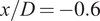
$ x/D=-0.6 $
 and
$ x/D=0 $
 . Also, in
$ x/D=0 $
 , neither
$ {u}_x $
 nor
$ {u}_y $
 matches with the asymptotic value of
$ {\boldsymbol{u}}_{\boldsymbol{ib}}=\left({U}_{\mathrm{max}},0\right) $
 inside the cylinder region
$ y\in \left[-D/2,D/2\right] $
 .
Velocity profiles when
$ \Delta \phi =\pi $
 at three different planes
$ x/D\in \left[-\mathrm{0.6,0,0.6}\right] $
 for (
 )
$ {\alpha}_p=40 $
 , (
 )
$ {\alpha}_p=4 $
 , and (
 )
$ {\alpha}_p=0.4 $
 . The three simulations are performed with a resolution
$ \Delta \mathbf{x}=D/25 $
 . (Ο) represents the data from the experiments conducted in Dütsch et al. (Reference Dütsch, Durst, Becker and Lienhart1998).

Figure 5. Long description
The figure consists of six panels arranged in two rows and three columns. All panels share a vertical axis labeled y forward slash D ranging from minus 1.0 to 1.0. The top row, panels (a), (b), and (c), shows horizontal velocity profiles u sub x all over U sub max. The bottom row, panels (d), (e), and (f), shows vertical velocity profiles u sub y all over U sub max.
Each column represents a different plane: x forward slash D equals minus 0.6 (left), x forward slash D equals 0 (center), and x forward slash D equals 0.6 (right). All panels include a Delta phi equals pi condition, indicating that the curves are estimated for this phase difference.
Data series in each panel include:
* Open circles: Experimental data from Dütsch et al. (1998).
* Solid red line: Simulation with alpha sub p equals 4.
* Dotted green line: Simulation with alpha sub p equals 0.4.
* Solid yellow line: Simulation with alpha sub p equals 40.
In panels (a), (b), (d), and (f), the red and green lines closely overlap and match the experimental circles, while the yellow line shows significant deviation, particularly in peak magnitudes. In panel (c), the yellow line shows a narrower peak compared to the other series. In panel (e), the yellow line exhibits a distinct oscillatory pattern not seen in the experimental data or the lower alpha sub p simulations.
Results for the investigation of the resistive force
$ {F}_x $
 are shown in Figure 6(a). Data are represented here in the reference frame of the force acting on the body by the fluid, which is the additive inverse of the forcing term defined in (3.4) and (3.5). One could say that the simulation with
$ {\alpha}_p=4 $
 best aligns with the experimental data since
$ {\alpha}_p=0.4 $
 provokes meaningful discontinuities between the solid and the fluid regions that cause significant noise in the
$ {F}_x $
 curve estimation. The results from the simulation with
$ {\alpha}_p=40 $
 are very smooth, but they present discrepancies in some specific phases of the oscillation. In Figure 6(b), we represent the spectra of the resistive force and compare it with a body-fitted simulation described in Tsetoglou et al. (Reference Tsetoglou, Cailler, Bénard, Lartigue, Moureau and Réveillon2024). One can see that all IBM simulations exhibit high-frequency noise, a well-known problem for IBM that has already been documented in the literature (Mittal and Iaccarino, Reference Mittal and Iaccarino2005). However, a concern arises when studying the low frequencies. All simulations correctly predict the peaks estimated with the body-fitted run, particularly the maximum peak located at
$ f=0.2\hskip0.22em Hz $
 , but only the simulation with
$ {\alpha}_p=40 $
 complies with the spectrum of the body-fitted run. The spectra are computed by using the 1D discrete Fourier transform (
$ DFT $
 ) (Press et al., Reference Press, Teukolsky, Vetterling and Flannery2017), but they are sped up with the fast Fourier transform (
$ FFT $
 ) algorithm (Cooley and Tukey, Reference Cooley and Tukey1965):

(a) Resistive force
$ {F}_x $
 over one period
$ T $
 , and (b) frequency resistive force spectra. The simulations represented are (
 )
$ {\alpha}_p=40 $
 , (
 )
$ {\alpha}_p=4 $
 , and (
 )
$ {\alpha}_p=0.4 $
 . The three simulations are performed with a grid resolution
$ \Delta \mathbf{x}=D/25 $
 . (Ο) represents the data from the experiments conducted in Dütsch et al. (Reference Dütsch, Durst, Becker and Lienhart1998) and (
$ \blacksquare $
 ) is a body-fitted simulation run in Tsetoglou et al. (Reference Tsetoglou, Cailler, Bénard, Lartigue, Moureau and Réveillon2024).

Figure 6. Long description
Panel a is a line graph of resistive force F sub x in Newtons versus normalized time tau over T from 0 to 1.0. A green jagged line for alpha sub p = 0.4 shows high-frequency oscillations around a sinusoidal trend. A dark red line for alpha sub p = 4 and a yellow line for alpha sub p = 40 follow smoother sinusoidal paths. White circles representing experimental data from Dütsch et al. and align closely with the alpha sub p = 4 and 40 curves. Panel b is a frequency spectrum graph showing the absolute value of the FFT of F sub x in Newtons versus frequency f in Hertz on a log-log scale from 10 super minus 2 to 10 super 2. It features prominent peaks at approximately 0.2 Hertz. The alpha sub p = 0.4 green data shows a high noise floor at higher frequencies. Black squares representing body-fitted simulations from Tsetoglou et al. show discrete peaks that align with the primary peaks of the alpha sub p = 40, 4 and 0.4 simulations before tapering off.
$ L=100\ 000 $
 is the total number of samples or window length, equivalent to
$ 50T $
 . The frequencies are given by
$ {f}_k=k/\left(\Delta tL\right) $
 for the kth index.
The sensitivity to the grid resolution
$ \Delta \boldsymbol{x} $
 is studied next. Simulations are run for
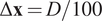
$ \Delta \boldsymbol{x}\in \left[D/25,D/40,D/100\right] $
 , while keeping
$ {\alpha}_p=0.4 $
 and
$ \Delta t=0.0025\hskip0.1em {t}_A $
 . Concerning the velocity profiles shown in Figure 7, they exhibit no significant discrepancies among the different resolutions, with all correctly capturing the expected physics of the test case (penalization of the velocity to its imposed value and symmetry about
$ y=0 $
 ). However, a slight improvement is observed for the fine-grained run with
$ \Delta \boldsymbol{x}=D/100 $
 , particularly noticeable in Figure 7(c) and (f) for the plane
$ x/D=0.6 $
 . The resistive force
$ {F}_x $
 in Figure 8(a) shows that all curves are capable of following the experimental data, but the presence of noise is clearly related to the degradation of the mesh. About the spectra in Figure 8(b), high-frequency noise decreases in strength with the reduction of the grid spacing.
Velocity profiles when
$ \Delta \phi =\pi $
 at three different planes
$ x/D\in \left[-\mathrm{0.6,0,0.6}\right] $
 for (
 )
$ \Delta \mathbf{x}=D/100 $
 , (
 )
$ \Delta \mathbf{x}=D/40 $
 , and (
 )
$ \Delta \mathbf{x}=D/25 $
 . The three simulations are performed with
$ {\alpha}_p=0.4 $
 . (Ο) represents the data from the experiments conducted in Dütsch et al. (Reference Dütsch, Durst, Becker and Lienhart1998).

Figure 7. Long description
A multi-panel figure with six graphs labeled a through f. All graphs share a vertical axis y forward slash D ranging from minus 1.0 to 1.0. The top row, panels a, b, and c, have a horizontal axis u sub x forward slash U sub max ranging from minus 1.0 to 1.0. The bottom row, panels d, e, and f, have a horizontal axis u sub y forward slash U sub max ranging from minus 1.0 to 1.0.
* Panel a: x forward slash D equals minus 0.6. Shows a wide, positive velocity peak between y forward slash D equals minus 0.5 and 0.5, with smaller negative peaks at the extremes.
* Panel b: x forward slash D equals 0. Shows a sharp, rectangular positive velocity profile between y forward slash D equals minus 0.5 and 0.5.
* Panel c: x forward slash D equals 0.6. Shows a single positive parabolic peak centered at y forward slash D equals 0.
* Panel d: x forward slash D equals minus 0.6. Shows an oscillating profile with four distinct peaks.
* Panel e: x forward slash D equals 0. Shows a near-zero velocity profile with minor fluctuations.
* Panel f: x forward slash D equals 0.6. Shows a sinusoidal profile with a negative peak at y forward slash D equals minus 0.3 and a positive peak at y forward slash D equals 0.3.
In all panels, open circles represent experimental data, while solid blue, solid orange, and dotted green lines represent simulations with varying grid resolutions Delta x equals D forward slash 100, D forward slash 40, and D forward slash 25 respectively. The simulation lines closely overlap and generally follow the experimental data points.
(a) Resistive force
$ {F}_x $
 over one period
$ T $
 , and (b) frequency resistive force spectra. The simulations represented are (
 )
$ \Delta \mathbf{x}=D/100 $
 , (
 )
$ \Delta \mathbf{x}=D/40 $
 , and (
 )
$ \Delta \mathbf{x}=D/25 $
 . The three simulations are performed with
$ {\alpha}_p=0.4 $
 . (Ο) represents the data from the experiments conducted in Dütsch et al. (Reference Dütsch, Durst, Becker and Lienhart1998) and (
$ \blacksquare $
 ) is a body-fitted simulation run in Tsetoglou et al. (Reference Tsetoglou, Cailler, Bénard, Lartigue, Moureau and Réveillon2024).

Figure 8. Long description
Panel a displays a line graph of resistive force F sub x in Newtons versus normalized time tau over T. The x-axis ranges from 0 to 1.0, and the y-axis ranges from -4 to 4. A smooth blue line with white circular markers represents experimental data, showing a sinusoidal wave that peaks at approximately 2.0 Newtons near tau over T equals 0.8 and troughs at -2.0 Newtons near 0.3. Three simulation datasets are overlaid. The green line (Delta x = D/25) shows the highest oscillation/noise around the mean path. The orange line (Delta x = D/40) shows moderate noise. The blue line (Delta x = D/100) is the smoothest.
Panel b displays the frequency resistive force spectra on a log-log scale. The x-axis is frequency f in Hertz ranging from 10-2 to 10 to the power of 2. The y-axis is the magnitude of the Fast Fourier Transform of F sub x in Newtons, ranging from 10 to the power of -9 to 10 to the power of 0. Black squares represent body-fitted simulation data, showing distinct peaks at 0.2, 0.6, and 1.0 Hertz before decaying. The simulation lines (green, orange, and blue) show a primary sharp peak at 0.2 Hertz. Beyond 1 Hertz, the simulations exhibit significant high-frequency noise floor divergence, with the green line (D/25) maintaining the highest noise level and the blue line (D/100) showing the lowest magnitude at high frequencies.
This parametric study indicates that, in general, lower values of
$ {\alpha}_p $
 and finer mesh resolutions
$ \Delta \boldsymbol{x} $
 yield the best flow conditions in terms of velocity and force profiles. However, higher values
$ {\alpha}_p $
 provide greater stability, particularly by reducing noise in the force profiles, improving the representation of the low-frequency spectrum, and attenuating the high-frequency range. Therefore, in the DA experiment described in Section 4, the objective is to optimize
$ {\alpha}_p $
 to simultaneously enhance flow conditions and accurately capture the resistive force spectrum.
4. Data assimilation experiment
In this section, we consider two simulations from the database described in Section 3.1. First, the simulation with
$ {\alpha}_p=0.4 $
 and
$ \Delta \boldsymbol{x}=D/100 $
 serves as a reference, from which
$ 16 $
 high-fidelity observations are extracted from
$ 8 $
 local sensors that measure both the streamwise
$ {u}_x $
 and crosswise
$ {u}_y $
 velocities. As one can see in Figure 9(a), the
$ 8 $
 sensors are strategically selected to help ensure the symmetry condition around
$ y=0 $
 . This simulation is referred to as HF-IBM (high-fidelity IBM). The second simulation, in which
$ {\alpha}_p=40 $
 and
$ \Delta \boldsymbol{x}=D/25 $
 , represents the prior condition for the state estimation of our assimilation experiment. This simulation was observed to exhibit problems in ensuring proper conditions for the velocity and force profiles; therefore, DA is used here to improve its performance. This simulation is referred to as LF-IBM (low-fidelity IBM). An EnKF with
$ {N}_e=40 $
 ensemble members is employed to carry out the assimilation, which uses the CONES library (Villanueva et al., Reference Villanueva, Valero, Šarkić-Glumac and Meldi2024b) adapted for OpenFOAM solvers and available at https://gitlab.ensam.eu/pe431/cones-dev. CONES provides a framework for performing online, ensemble-based DA at runtime, enabling continuous corrections to fields and model parameters without interrupting or restarting the simulation. The step-by-step procedure specific to the present study is described in Appendix A. A total number of
$ K=2\hskip0.1em 500 $
 analysis phases over a total time window of
$ 50\hskip0.2em T $
 are performed, with constantly spaced assimilation windows of
$ 40\Delta t $
 . The uncertainty prescribed for the observations (i.e., their standard deviation) is set to
$ 0.05\hskip0.1em {U}_{\mathrm{max}} $
 , which is a plausible value for realistic applications.
(a) Location of the high-fidelity observation with respect to the position of the cylinder when its center
$ \left({x}_{ib},{y}_{ib}\right)=\left(0,0\right) $
 , and (b) definition of all the constraints for the penalization time-step parameter
$ {\alpha}_p $
 as a function of the radial position.

Figure 9. Long description
Panel a shows a heat map of velocity magnitude around a red central cylinder. A color bar at the top ranges from 1.4e-04 in dark blue to 1.1e+00 in dark red. The flow wake is visible as a teardrop-shaped red region behind the cylinder, surrounded by yellow and green gradients. Small white dots indicate observation points. Panel b is a line graph with the y-axis labeled 1 all over alpha sub p delta t and the x-axis labeled r. The graph is divided into three regions. The first region, shaded blue, extends from the origin (x sub i b, y sub i b) to r sub min = D all over 4. It contains a horizontal white line with constraints 1) alpha sub p at r sub min = 40 and 2) the derivative of the y-axis expression with respect to r at r sub min = 0. The second region, shaded purple, extends to r star and shows the white line curving upward to a peak. Constraints 3) and 4) indicate alpha sub p at r star equals alpha sub p super min and the derivative at r star equals 0. The third region, shaded red, extends to D all over 2 where the curve descends. Constraint 5) shows the limit as r approaches (D all over 2 + delta x) from the left of alpha sub p equals positive infinity. Below the x-axis, the regions are grouped into Omega sub b and Omega sub f.
Regarding the ensemble’s variability, since the flow is laminar, perturbing only some of the model’s parameters would not be sufficient. Thus, the perturbation is also applied to the physical field (i.e., velocity field
$ \boldsymbol{u} $
 ). To achieve this,
$ 40 $
 instantaneous velocity snapshots from the LF-IBM run over a single period
$ T $
 serve as initial conditions for each ensemble member. As a result, each realization of the ensemble starts with a different phase in the cycle/initial position of the cylinder (
$ {x}_0,{y}_0 $
 ). The purpose of the DA experiment is to reduce the ensemble’s variability in order to identify a suitable state estimation that complies with the observations in a probabilistic sense. This is obtained here via the optimization of a set of free parameters
$ \theta $
 . Determining these parameters allows the ensemble of realizations to synchronize with the high-fidelity observations. In this context, the cylinder’s initial position in the streamwise direction,
$ {x}_0 $
 , is treated as a free parameter to be inferred by the EnKF. Consequently, the cylinder’s position becomes a dynamic variable influenced by the DA algorithm, which must be accounted for within the PISO algorithm (see Algorithm 1). Additionally, the value of
$ {\alpha}_p $
 is locally optimized. This variable is expressed via an expansion in the radial direction
$ r=\sqrt{{\left(x-{x}_{ib}\right)}^2+{\left(y-{y}_{ib}\right)}^2} $
 which, unlike the azimuthal coordinate
$ \Theta =\arctan \left(y-{y}_{ib}\right)/\left(x-{x}_{ib}\right) $
 , does not depend on the oscillation phase. This phase-independence allows us to assume
$ {\alpha}_p\ne {\alpha}_p(t) $
 , thereby simplifying the assimilation procedure within the EnKF framework. This function presents the following shape:

The choice for the expansion describing
$ 1/\left({\alpha}_p\Delta t\right) $
 provides a more flexible parametric space. The coefficients
$ {a}_j,\ j\in \left(0,\dots, 4\right) $
 in (4.1) will converge to time-independent values through the assimilation procedure and are computed through an algebraic operation based on the optimized parameters
$ {\theta}_k^a $
 estimated via the EnKF. While these model parameters remain constant over time, the state estimation procedure dynamically corrects the flow field, thereby capturing the system’s inherent unsteady behavior through the assimilation of instantaneous observations. These coefficients capture information about the critical points of the radial expansion
$ \left(\frac{\partial \left(1/\left({\alpha}_p\Delta t\right)\right)}{\partial r}=0\right) $
 . A fourth-degree polynomial is employed to enforce five specific constraints. The detailed formulation of both the parameters and the conditions they satisfy is presented next. First, the LF-IBM simulation achieved the desired resistive spectrum at low frequencies. Then, we define an inner region of the cylinder
$ r<{r}_{\mathrm{min}} $
 (corresponding to the blue region in Figure 4(b)) where
$ {\alpha}_p $
 is kept constant and equal to its LF-IBM value,
$ {\alpha}_p=40 $
 . This condition ensures that the low-frequency noise in the resistive force
$ {F}_x $
 remains consistent with the body-fitted simulation spectrum. Later, when
$ r\ge {r}_{\mathrm{min}} $
 , we allow for a smooth transition of
$ {\alpha}_p $
 to let the value evolve toward a minimum
$ {\alpha}_p^{\mathrm{min}} $
 , expected to approach
$ {\alpha}_p=0.4 $
 , so the simulations match the HF-IBM observations. Last, we want that
$ \underset{r\to {\left(D/2+\Delta \boldsymbol{x}\right)}^{-}}{\lim }{\alpha}_p=+\infty $
 to reduce the discontinuity between the fluid and the solid regions. One can see that the limit considers the size of the additional cell layer represented in red in Figure 4(b). A sketch of all the constraints with the function
$ 1/\left({\alpha}_p\Delta t\right) $
 is represented in Figure 9(b), with the distinction between the zone where
$ {\alpha}_p $
 does not change (in blue), the zone affected by the polynomial within the cylinder (in purple), and the additional external cell layer (in red). Since OpenFOAM solves the Navier–Stokes equations in the Cartesian coordinate framework, we optimize, separately, the radius
$ {r}^{\ast } $
 and
$ {\alpha}_p^{\mathrm{min}} $
 for each component of the forcing term
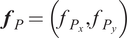
$ {\boldsymbol{f}}_P=\left({f}_{P_x},{f}_{P_y}\right) $
 , and we employ their values to recalculate the coefficients of the polynomial expansion written in (4.1) at each analysis phase
$ k $
 up to convergence. The application of this strategy for the IBM forcing required the optimization of five model parameters, which are grouped in the vector
$ \theta =\left\{{x}_0,{r}_x^{\ast },{\alpha}_{p_x}^{\mathrm{min}},{r}_y^{\ast },{\alpha}_{p_y}^{\mathrm{min}}\right\} $
 . The matrix formulation used to compute the coefficients
$ {a}_j $
 at each assimilation phase is presented in (4.2), where the sub-index
$ i=\left(x,y\right) $
 denotes the corresponding spatial direction.

The prior for
$ {r}^{\ast } $
 and
$ {\alpha}_p^{\mathrm{min}} $
 in the two directions correspond to normal distributions such as
$ {r}^{\ast }=\mathcal{N}\left(\frac{3D}{8},{\left(0.05\frac{3D}{8}\right)}^2\right) $
 and
$ {\alpha}_p^{\mathrm{min}}=\mathcal{N}\left(40,4\right) $
 . For the former, the average lies between
$ {r}_{\mathrm{min}}=D/4 $
 and the cylinder’s boundary at
$ D/2 $
 , with a standard deviation of
$ 5\% $
 among ensemble members. For the latter, the average is set to the value imposed at
$ r<{r}_{\mathrm{min}} $
 , with a variability of again
$ 5\% $
 .
4.1. Results
The analysis of the performance of the DA experiment includes an investigation of several flow quantities. First, we examine the vorticity
$ \omega =\mathbf{\nabla}\times \boldsymbol{u} $
 when the phase difference
$ \Delta \phi =0 $
 , that is,
$ {u}_{ib_x}=-{U}_{\mathrm{max}} $
 . In Figure 10, one can see that the DA-IBM run outperforms the prior LF-IBM simulation, closely matching the high-fidelity HF-IBM results. Minor perturbations, mostly near the leading edge, are observed, which may be associated with the coarser mesh resolution. However, this does not prevent the results obtained with DA from recovering the symmetry condition at
$ y=0 $
 , which was lost in the LF-IBM run.
Vorticity contours
$ {\omega}_z $
 when
$ \Delta \phi =0 $
 for (a) the prior LF-IBM, (b) the reference simulation from which we obtain the high-fidelity data HF-IBM, (c) the experiment with Data Assimilation DA-IBM, and (d) the experiment performed by Dütsch et al. (Reference Dütsch, Durst, Becker and Lienhart1998).

Figure 10. Long description
The figure consists of four panels labeled a through d, each showing a central cylinder with contour lines representing fluid flow.
Panel a, labeled L F minus I B M, shows a cylinder with rough, widely spaced contour lines forming an asymmetric wake that extends to the right. Small isolated loops appear to the far left and right.
Panel b, labeled H F minus I B M, shows the cylinder with much denser, more tightly packed contour lines concentrated near the surface of the cylinder, particularly on the top and bottom edges, indicating higher fidelity gradients.
Panel c, labeled D A minus I B M, displays a contour pattern very similar to panel b, with high-density lines hugging the cylinder surface and a structured wake trailing to the right, even if it keeps rough contour lines akin to panel a.
Panel d, labeled Dütsch et al., shows the experimental reference. The surrounding contours are dense near the cylinder surface, similar to panels b and c.
Second, we represent the velocity profiles at three different planes again when the phase difference
$ \Delta \phi =\pi $
 , as illustrated in Figure 11. Again, the DA-IBM run is symmetric around
$ y=0 $
 and properly constrains the velocity within the solid region. In particular, the condition at
$ x/D=0 $
 , in which
$ \left({u}_x,{u}_y\right)=\left({U}_{\mathrm{max}},0\right) $
 is satisfied within the cylinder
$ y\in \left[-D/2,D/2\right] $
 . Overall, the velocity profiles from the DA-IBM run closely match those from the HF-IBM simulation. Additionally, we represent the profiles at
$ \Delta \phi =7\pi /6 $
 in Figure 12, which corresponds to a cylinder position at
$ {x}_{ib}/D=0.4 $
 and velocity
$ {u}_{x_{ib}}/{U}_{\mathrm{max}}=0.87 $
 . In this case, one can see how DA profiles nearly overlap those from the HF-IBM run, demonstrating a clear improvement over the LF-IBM profiles. The only noticeable exception occurs in
$ {u}_x $
 for the plane
$ x/D=0.6 $
 , where the LF-IBM solution shows slightly better agreement above the cylinder compared to the experimental data; however, it still fails to preserve the symmetry with respect to
$ y=0 $
 , so the velocity profiles represented in HF-IBM and DA-IBM runs are physically more consistent and reliable.
Velocity profiles when
$ \Delta \phi =\pi $
 at three different planes
$ x/D\in \left[-\mathrm{0.6,0,0.6}\right] $
 for (
 ) the DA-IBM experiment, (
 ) the HF-IBM run, and (
 ) the LF-IBM simulation. (Ο) represents the data from the experiments conducted in Dütsch et al. (Reference Dütsch, Durst, Becker and Lienhart1998).

Figure 11. Long description
The multi-panel graph is organized into two rows. The top row, panels a, b, and c, plots y all over D on the vertical axis against u sub x all over U max on the horizontal axis. The bottom row, panels d, e, and f, plots y all over D against u sub y all over U max.
Each column represents a different plane: x all over D equals minus 0.6 for panels a and d, x all over D equals 0 for panels b and e, and x all over D equals 0.6 for panels c and f. All panels share a constant Delta phi equals pi.
Data is represented by four distinct styles:
1. Open circles for experimental data from Dütsch et al. 1998.
2. A solid blue line for the H F - I B M run.
3. A solid yellow line for the L F - I B M simulation.
4. A dotted grey line for the D A - I B M experiment.
In the top row, the streamwise velocity profiles show a prominent central peak near y all over D equals 0 in panel a, which transitions into a wide plateau in panel b, and a narrower peak in panel c. The solid blue and dotted grey lines closely follow the experimental circles, while the solid yellow line shows significant deviation, particularly in panel b where it fails to reach the same plateau width.
In the bottom row, the crosswise velocity profiles exhibit larger oscillatory behavior. In panel d, the data shows four distinct peaks. In panel e, apart from the solid yellow line, which deviates significantly, the profiles are nearly vertical near zero with small fluctuations. In panel f, two peaks are observed. Across these panels, the solid blue and dotted grey lines maintain high alignment with the experimental data, while the solid yellow line consistently overshoots or undershoots the two peaks.
Velocity profiles when
$ \Delta \phi =7\pi /6 $
 at three different planes
$ x/D\in \left[-\mathrm{0.6,0,0.6}\right] $
 for (
 ) the DA-IBM experiment, (
 ) the HF-IBM run, and (
 ) the LF-IBM simulation. (Ο) represents the data from the experiments conducted in Dütsch et al. (Reference Dütsch, Durst, Becker and Lienhart1998).

Figure 12. Long description
The figure consists of six panels labeled a through f. The top row (a, b, c) shows normalized horizontal velocity u sub x all over U max on the x-axis against normalized vertical position y all over D on the y-axis. The bottom row (d, e, f) shows normalized vertical velocity u sub y all over U max on the x-axis against y all over D. All panels share a y-axis range from -1.0 to 1.0 and an x-axis range from -1.0 to 1.0, with a constant delta phi of 7 pi over 6
* Panel a: x all over D equals -0.6. The velocity profile shows a large positive peak near y equals 0. The H F I B M (solid blue line) and DA I B M (dotted gray line) closely match the experimental circles, while the LF I B M (solid yellow line) overshoots the peak and deviates significantly at y equals 0.7.
* Panel b: x all over D equals 0. The profile is a broad plateau from y equals -0.4 to 0.4. All simulation lines closely follow the experimental circles.
* Panel c: x all over D equals 0.6. The profile shows a sharp rectangular velocity block between y equals -0.5 and 0.5. All simulations show issues to follow the experimental data outside the cylinder region.
* Panel d: x all over D equals -0.6. The vertical velocity shows an S-shaped curve. The yellow line is shifted slightly to the right of the blue lines and experimental circles.
* Panel e: x all over D equals 0. All profiles are near zero with small fluctuations. The yellow line does not respect the central symmetry.
* Panel f: x all over D equals 0.6. The profiles show two small peaks near y equals -0.5 and 0.5.
We present the interaction or resistive force
$ {F}_x $
 over a single period
$ T $
 in Figure 13 again. The DA-IBM profile matches the HF-IBM simulation with high precision, with just some slight discrepancies in the acceleration parts within the period (
$ d\left(\mathrm{mag}\left({\boldsymbol{u}}_{\boldsymbol{ib}}\right)\right)/ dt>0 $
 ), specifically when
$ \tau /T\in \left[\mathrm{0.25,0.5}\right] $
 and
$ \tau /T\in \left[\mathrm{0.75,1}\right] $
 , corresponding to
$ \Delta \phi \in \left[\pi /2,\pi \right] $
 and
$ \Delta \phi \in \left[-\pi /2,0\right] $
 , respectively. In any case, these discrepancies are smaller than the differences in the deceleration phases (
$ d\left(\mathrm{mag}\left({\boldsymbol{u}}_{\boldsymbol{ib}}\right)\right)/ dt<0 $
 ) in the LF-IBM simulation for
$ \tau /T\in \left[\mathrm{0,0.25}\right] $
 and
$ \tau /T\in \left[\mathrm{0.5,0.75}\right] $
 , that is,
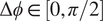
$ \Delta \phi \in \left[0,\pi /2\right] $
 and
$ \Delta \phi \in \left[-\pi, -\pi /2\right] $
 . Regarding the spectral analysis, in the DA method combined with the radial expansion of
$ {\alpha}_p(r) $
 , low frequencies are better captured since
$ {\alpha}_p $
 is left to the stable value
$ {\alpha}_p=40 $
 within the central part of the cylinder (
$ r<{r}_{\mathrm{min}} $
 ), and the high-frequency noise observed matches the equivalent noise observed in Figure 6
(b) for the run with
$ {\alpha}_p=0.4 $
 and grid refinement of
$ \Delta \boldsymbol{x}=D/25 $
 . In fact, as shown in Table 1, the averaged value from all ensemble members
$ \left(\overline{\cdot}\right) $
 for the minimum value
$ {\alpha}_P^{\mathrm{min}} $
 obtained with DA in both directions
$ x $
 and
$ y $
 is very close to the
$ {\alpha}_p=0.4 $
 value from the HF-IBM run, with this maximum occurring near the initial condition described in Section 4 at
$ r/D=3/8 $
 .
(a) Resistive force
$ {F}_x $
 over one period
$ T $
 , and (b) frequency resistive force spectra. The simulations represented are (
 ) DA-IBM, (
 ) HF-IBM, and (
 ) LF-IBM. (Ο) represents the data from the experiments conducted in Dütsch et al. (Reference Dütsch, Durst, Becker and Lienhart1998) and (
$ \blacksquare $
 ) is a body-fitted simulation run in Tsetoglou et al. (Reference Tsetoglou, Cailler, Bénard, Lartigue, Moureau and Réveillon2024).

Figure 13. Long description
Panel a is a line graph of resistive force F sub x in Newtons versus normalized time tau over T from 0 to 1.0. The data shows a sinusoidal oscillation. The D A I B M (gray line) and H F I B M (blue line) closely follow the experimental data points (white circles).
Panel b is a frequency spectrum graph showing the magnitude of the Fast Fourier Transform of F sub x in Newtons on a logarithmic Y-axis from 10 super minus 9 to 10 super 0, against frequency f in Hertz on a logarithmic X-axis from 10 super minus 2 to 10 super 2.
- The D A I B MH F - I B M (blue line) shows a distinct peak at approximately 0.2 Hertz and maintains a lower noise floor at high frequencies.
- The H F I B MLF - IBM (yellow line) shows a similar peak but has a higher noise floor than D A I B MH F - I B M above 1 Hertz.
- The L F I B MD A - I B M (grey line) exhibits the highest noise floor, particularly in the 1 to 100 Hertz range.
- Black squares represent the body-fitted simulation, showing discrete peaks at 0.2, 0.6, and 1.0 Hertz.
Comparison between the parameters employed as a prior or initial condition in the DA experiment, and the values optimized after the DA experiment

Table 1. Long description
The table consists of three rows and six columns.
Row 1 (Header):
- Column 1: Empty.
- Column 2: Ensemble average of the cylinder position x sub 0 bar.
- Column 3: Ensemble average of the radius for which alphaPX is minimal r sub x super asterisk bar all over D.
- Column 4: Ensemble average of the minimal streamwise time-dependent penalization parameter alpha sub P sub x super min bar.
- Column 5: Ensemble average of the radius for which alphaPY is minimal r sub y super asterisk bar all over D.
- Column 6: Ensemble average of the minimal crosswise time-dependent penalization parameter alpha sub P sub y super min bar.
Row 2 (prior):
- Column 1: prior.
- Column 2: 0.
- Column 3: 0.375.
- Column 4: 40.
- Column 5: 0.375.
- Column 6: 40.
Row 3 (D A - I B M):
- Column 1: D A - I B M.
- Column 2: minus 1.8639 e super minus 4.
- Column 3: 0.3915.
- Column 4: 0.5310.
- Column 5: 0.3909.
- Column 6: 0.3716.
Finally, the differences observed in the vorticity fields suggest examining the lift force
$ {F}_y $
 and its spectral distribution, estimated using (3.6). As shown in Figure 14, the application of DA induces significant noise in the time evolution of
$ {F}_y $
 , which yields larger nonzero values. This observation is due to modifications in the flow state by the DA procedure, which introduces discontinuities in the lift signal. Results for the DA-IBM simulation, as shown in Figure 14(a), have been smoothed with a median filter (Tukey, Reference Tukey1974) with kernel size
$ 9 $
 to perform a clear comparison with the IBM runs, which are clearly less noisy than the DA-IBM simulation. The filtering intensity has been tuned so that the
$ 50 $
 peaks corresponding to the number of analysis steps performed over that interval remain observable. These large fluctuations in
$ {F}_x $
 and
$ {F}_y $
 are also observed in classical body-fitted and IBM CFD runs at the very beginning of the simulations, when initial conditions imposed may affect the calculation of integral quantities such as body forces. For this reason, it is recommended to filter time signals for these quantities when performing analysis phases, as we did in Figure 14(a). In the frequency domain, the low-frequency content of the DA-IBM solution remains within the range spanned by the LF-IBM and HF-IBM results. However, the dominant spectral peaks are shifted toward lower frequencies relative to LF-IBM, aligning instead with a characteristic frequency of the HF-IBM simulation.
(a) Lift force
$ {F}_y $
 over one period
$ T $
 , and (b) frequency lift force spectra. The simulations represented are (
 ) DA-IBM, (
 ) HF-IBM, and (
 ) LF-IBM.

Figure 14. Long description
Panel a is a line graph of lift force F sub y in Newtons versus normalized time tau all over T from 0 to 1.0. The vertical axis ranges from negative 0.05 to 0.05. The grey line (L F - I B MD A - I B M) shows high-amplitude, erratic oscillations throughout the period. The yellow line (H F - I B MLF - IBM) and blue line (D A - I B MH F - I B M) remain relatively flat near zero with some occasional sharp, localized spikes.
Panel b is a frequency spectrum graph on a log-log scale. The horizontal axis is frequency f in Hertz from 10 super negative 2 to 10 super 2. The vertical axis is the magnitude of the F F T of F sub y in Newtons from 10 super negative 9 to 10 super negative 3. The blue line (D A-I B MH F - I B M) is the lowest, showing distinct peaks at 0.2 and 0.4 Hertz before decaying into a noisy floor. The yellow line (H F - I B MLF - IBM) is higher, with prominent peaks at 0.4 and 0.8 Hertz. The grey line (L F - I B M) possesses the same main frequency as H F - I B M and shows a dense, high-amplitude noise profile that stays above 10 super negative 6 even at high frequencies.
5. Machine learning experiment
This section outlines the use of DA-augmented profiles to construct black-box ML models that integrate a sliding-window strategy with the RFR algorithm to learn the parameter optimization process of the DA framework. Throughout this work, because the ML components operate on DA outputs, the models are trained and applied under the assumption that the relevant flow information (specifically, the velocity field and the oscillation cycle) is already available from the preceding DA stage. The methodology is demonstrated for the oscillating-cylinder case using the penalty forcing term
$ {\boldsymbol{f}}_P $
 . As defined in (2.3), this term is treated as a local field whose behavior is expected to vary with the oscillation phase. Accordingly, (i) separate models are developed for distinct phases of the oscillation cycle
$ \Delta \phi $
 , and (ii) suitable features must be identified to ensure an accurate characterization of
$ {\boldsymbol{f}}_P $
 . The work is performed on the assumption that the features of the unsteady behavior of the flow are known, as previously discussed. This permits training and using ML tools over well-defined time windows, which is clearly a strong simplification relative to real flows, where unsteady variations are unknown and must be accounted for online. However, this simplified analysis can highlight the potential for coupling DA and ML, particularly the numerical and algorithmic difficulties that need to be addressed.
Concerning the first listed point (i.e., generation of separate models), we train five ML models online to capture different flow dynamics across the oscillation cycle (i.e., flow acceleration, deceleration, and direction changes) using streaming data during the assimilation procedure. Since the regime under consideration is laminar, the training data consists of the assimilated fields within the solid region
$ {\Omega}_b $
 over a single oscillation cycle, comprising approximately
$ 550 $
 mesh elements at each time step, extracted for the
$ {N}_e=40 $
 ensemble members. Additionally, to avoid abrupt interruptions in predictions at model boundaries, we employ a sliding window approach with a sliding period
$ {p}_{SW}=0.5{T}_W $
 , where the window size
$ {T}_W=2T/5 $
 is uniform across the five models. Hence, the first model is trained on data from
$ \tau /T\in \left(\mathrm{0,0.4}\right] $
 , the second on
$ \tau /T\in \left(\mathrm{0.2,0.6}\right] $
 , the third on
$ \tau /T\in \left(\mathrm{0.4,0.8}\right] $
 , the fourth on
$ \tau /T\in \left(\mathrm{0.6,1}\right] $
 , and the last one on
$ \tau /T\in \left(\mathrm{0,0.2}\right]\cup \tau /T\in \left(\mathrm{0.8,1}\right] $
 . By sampling data every
$ 10\Delta t $
 time steps (half immediately following the assimilation phase and half midway between successive phases since the assimilation step has been decreased up to
$ 20\Delta t $
 for data collection), each black-box model is trained with approximately
$ {m}_T\approx 1.76M $
 samples, which is generally sufficient to ensure convergence of the RFR algorithm (Valero and Meldi, Reference Valero and Meldi2025b). Of these samples,
$ 80\% $
 are explicitly used for training, and
$ 20\% $
 are employed for validation. The remaining hyperparameters include the number of decision trees, set to
$ N=100 $
 , and the minimum number of samples per leaf node, set to
$ {m}_{sl}=5 $
 , ensuring robustness against overfitting. Each model is subsequently applied only within the central portion of its corresponding window, that is, for
$ \tau /T\in \left({\tau}_{\mathrm{init}}/T+{T}_W/4,{\tau}_{\mathrm{end}}/T-{T}_W/4\right] $
 , with
$ {\tau}_{\mathrm{init}}/T $
 and
$ {\tau}_{\mathrm{end}}/T $
 the initial and final times for each training window, respectively, and where predictive accuracy is expected to be highest. Integration with OpenFOAM is facilitated by the C++ library dlib (King, Reference King2009), which provides strong modularity within OpenFOAM solvers. Figure 15 illustrates all these concepts.
Sliding-window approach for the oscillating cylinder, where each green rectangle represents a different window during training, and blue rectangles indicate the utilization sequence of the models during the prediction of the penalty forcing term
$ {\boldsymbol{f}}_P $
 .

Figure 15. Long description
The diagram is divided into two main sections: TRAINING and TESTING.
At the top left, an equation defines the velocity ratio u sub i b x over U sub max as equal to minus cos open parenthesis 2 pi tau over T close parenthesis.
The TRAINING section features a line graph with a vertical axis for velocity ratio and a horizontal axis for tau over T ranging from 0 to 1. A red cosine curve oscillates across the graph. Overlaid on this curve are five overlapping green rectangles representing sliding windows, labeled R F R model 1 through R F R model 5. It is observed that for the specific case of 5 RFR models, the ratio between the overlapping period pSW and the window width TW is 0.5.
The TESTING section at the bottom shows a horizontal sequence of six blue rectangles. Each rectangle contains a penalty forcing term f hat sub P with subscripts 5, 1, 2, 3, 4, and 5 respectively. Below these, a horizontal axis for tau over T is marked with intervals 0.1, 0.3, 0.5, 0.7, and 0.9. Each interval is aligned with a specific model label: R F R model 5, R F R model 1, R F R model 2, R F R model 3, R F R model 4, and R F R model 5.
Regarding the feature selection, we recall that in the DA optimization procedure, the penalty forcing term
$ {\boldsymbol{f}}_P $
 is a local field which, for a given mesh element, depends solely on the local flow velocity
$ \boldsymbol{u} $
 , the prescribed cylinder motion
$ {\boldsymbol{u}}_{\boldsymbol{ib}} $
 , and the radial distance
$ r $
 (through
$ {\alpha}_P={\alpha}_P(r) $
 ). At first glance, these quantities appear to provide a sufficient set of input features for the ML model. However, predictions generated by black-box ML models often contain residual noise. In a laminar regime, where the flow exhibits limited inherent physical dissipation, such errors are unlikely to be smoothed out by the flow dynamics and could instead accumulate over time. This issue is particularly critical in the present framework, as the PISO algorithm computes (via calls to the ML models) an explicit forcing term
$ {\hat{\boldsymbol{f}}}_P $
 three times per time step: once during the predictor stage and twice during the correction stages after each velocity update (see Algorithm 2). From this point onward, the hat symbol (
$ \hat{\cdot} $
 ) indicates quantities predicted by the ML models. Repeated evaluations of
$ {\hat{\boldsymbol{f}}}_P $
 can potentially amplify errors in the fields introduced by previous ML predictions, leading to spurious flow gradients, especially near the domain boundaries.
To mitigate these effects, the boundary conditions are switched from zeroGradient to periodic (cyclic) on opposite sides of the domain. This modification ensures that both the flow field and its fluxes are continuous across boundaries, effectively preventing the artificial accumulation of momentum that might occur with nonperiodic (Neumann-type) boundaries. The cyclic formulation thus promotes smoother flow dissipation and yields a more physically consistent representation of the near-boundary dynamics, independent of the initial cylinder motion.
Additionally, inspired by the work by Villiers et al. (Reference Villiers, Mons, Sipp, Lamballais and Meldi2025), we enrich the input space with the cylinder acceleration
$ {\boldsymbol{a}}_{\boldsymbol{ib}} $
 , which is the time derivative of
$ {\boldsymbol{u}}_{\boldsymbol{ib}} $
 , and is incorporated to reinforce the phase difference
$ \Delta \phi $
 :

Furthermore, the inclusion of the vorticity
$ \omega $
 accounts for the velocity gradients between neighboring mesh elements. It is, however, counterproductive to introduce the time derivatives of the flow velocity, as the state estimation in the DA procedure introduces noise that increases exponentially with local accelerations, thereby degrading the performance of the black-box model. Since
$ {\boldsymbol{f}}_P=({f}_{P_x},{f}_{P_y}) $
 is a vector field, each component depends on the flow features along its respective direction. Consequently, two separate models are trained, one for each component of
$ {\boldsymbol{f}}_P $
 . The input features
$ \mathcal{X} $
 and target dependent variables
$ \mathcal{Y} $
 are normalized and defined as
$ {\mathcal{X}}_i=\left\{r/\left(D/2\right),{u}_i/{U}_{\mathrm{max}},{u}_{ib_x}/{U}_{\mathrm{max}},{a}_{ib_x}/\left({U}_{\mathrm{max}}f\right),{\omega}_z/f\right\} $
 and
$ {\mathcal{Y}}_i={\boldsymbol{f}}_{P_i}/\left({U}_{\mathrm{max}}f\right) $
 , respectively, where the sub-index
$ i=\left(x,y\right) $
 denotes the corresponding spatial direction.
Two metrics are employed to evaluate the quality of the black-box models on the validation dataset (comprising
$ 0.2{m}_T $
 samples): the coefficient of determination
$ {\mathcal{R}}^2 $
 and the normalized root MSE
$ \mathrm{or}\ \mathrm{NRMSE} $
 . Together, these metrics quantify both the variance explained by the model and the magnitude of the average prediction error. Their expressions are given by


where
$ j\in \left[\mathrm{1,0.2}{m}_T\right] $
 indexes the individual validation samples. For normalization, the metrics employ the mean of the reference data
$ \overline{\mathcal{Y}} $
 and the interquartile range
$ {Q}_3-{Q}_1 $
 , corresponding to the
$ 25 $
 th and
$ 75 $
 th percentiles of the true values
$ \mathcal{Y} $
 , which is advantageous due to its robustness against outliers. The results, summarized in Table 2, show consistently high
$ {\mathcal{R}}^2 $
 values and low
$ \mathrm{NRMSE} $
 levels, confirming the excellent predictive accuracy and generalization capability of all trained RFR models.
Metrics computed for the two components (
$ x,y $
 ) of the forcing term
$ {\boldsymbol{f}}_P $
 for each of the five RFR models employed

Table 2. Long description
The table consists of five columns and six rows including the header. The columns are labeled from left to right as: Model Name, N R M S E sub x, R super 2 sub x, N R M S E sub y, and R super 2 sub y.
* R F R model 1: N R M S E sub x is 0.053, R super 2 sub x is 0.997, N R M S E sub y is 0.014, R super 2 sub y is 1.
* R F R model 2: N R M S E sub x is 0.048, R super 2 sub x is 0.997, N R M S E sub y is 0.012, R super 2 sub y is 1.
* R F R model 3: N R M S E sub x is 0.051, R super 2 sub x is 0.998, N R M S E sub y is 0.016, R super 2 sub y is 1.
* R F R model 4: N R M S E sub x is 0.053, R super 2 sub x is 0.996, N R M S E sub y is 0.015, R super 2 sub y is 1.
* R F R model 5: N R M S E sub x is 0.045, R super 2 sub x is 0.999, N R M S E sub y is 0.015, R super 2 sub y is 1.
5.1. Validation in the reference oscillatory regime
In this section, we assess the performance of the sliding-window strategy under conditions identical to those of the training dataset. In this run, the original LF-IBM solver is solely enhanced with the RFR models constructed with the augmented data from the assimilation strategy for
$ 50 $
 oscillating periods, but no additional assimilation steps are performed during the present simulation. This configuration is referred to as ML-IBM. We begin by examining the velocity profiles at three planes for the phase differences
$ \Delta \phi =\pi $
 and
$ \Delta \phi =7\pi /6 $
 , as previously analyzed in Section 4.1. Figure 16 presents the profiles for
$ \Delta \phi =\pi $
 . The ML-IBM results nearly coincide with those obtained using the DA-IBM method and show a substantial improvement over the LF-IBM solution. Minor discrepancies with respect to DA-IBM appear in regions with pronounced velocity gradients, but these differences are negligible relative to the overall agreement. Figure 17 illustrates the case for
$ \Delta \phi =7\pi /6 $
 , where some limitations of the ML approach become evident. Although the ML-IBM results generally follow the DA-IBM trends and continue to outperform LF-IBM, the method struggles to accurately reproduce the wake structure behind the cylinder. This deviation is most apparent in Figure 17(b), where the velocity profile exhibits a parabolic shape (with reduced velocity near
$ y/D=0 $
 ) not captured by either the IBM or DA formulations. Nevertheless, this remains the only noticeable discrepancy, and overall, the ML-IBM results represent a marked improvement compared with the LF-IBM baseline.
Velocity profiles when
$ \Delta \phi =\pi $
 at three different planes
$ x/D\in \left[-\mathrm{0.6,0,0.6}\right] $
 for (
 ) the ML-IBM run, (
 ) the DA-IBM experiment, and (
 ) the LF-IBM simulation. (Ο) represents the data from the experiments conducted in Dütsch et al. (Reference Dütsch, Durst, Becker and Lienhart1998).

Figure 16. Long description
The figure consists of six panels arranged in two rows. The top row, panels a, b, and c, shows the normalized horizontal velocity u sub x over U max on the x-axis against the vertical position y over D on the y-axis. The bottom row, panels d, e, and f, shows the normalized vertical velocity u sub y over U max on the x-axis against y over D. All panels share a y-axis range from -1.0 to 1.0 with a uniform delta phi equal to pi.
* Panel a: At x over D equals -0.6, the horizontal velocity shows a large positive peak near y over D equals 0. The M L I B M (solid magenta line) and L F I B MD A-I B M (dotted grey line) closely match the experimental circles, while the D A I B MLF-IBM (solid yellow line) deviates significantly with a sharp negative peak near y over D equals 0.7.
* Panel b: At x over D equals 0, the horizontal velocity profile is nearly rectangular, peaking between y over D equals -0.5 and 0.5. Magenta and grey lines align with experimental data, while the yellow line shows a lower peak velocity.
* Panel c: At x over D equals 0.6, the profile shows a single positive peak centered at y over D equals 0. The yellow line is narrower and lower than the magenta and grey lines and experimental data.
* Panel d: At x over D equals -0.6, the vertical velocity oscillates. The magenta and grey lines follow the experimental data’s S-curve, while the yellow line is shifted to the right.
* Panel e: At x over D equals 0, the vertical velocity is near zero for most of the profile. The yellow line shows a distinct value within the solid region of the cylinder that is not present in the other datasets.
* Panel f: At x over D equals 0.6, the vertical velocity shows a negative peak at y over D equals -0.3 and a positive peak at y over D equals 0.3. The magenta and grey lines match the experimental data closely, while the yellow line underestimates the negative peak magnitude.
Velocity profiles when
$ \Delta \phi =7\pi /6 $
 at three different planes
$ x/D\in \left[-\mathrm{0.6,0,0.6}\right] $
 for (
 ) the ML-IBM run, (
 ) the DA-IBM experiment, and (
 ) the LF-IBM simulation. (Ο) represents the data from the experiments conducted in Dütsch et al. (Reference Dütsch, Durst, Becker and Lienhart1998).

Figure 17. Long description
A six-panel grid of line graphs labeled a through f. All graphs share a vertical axis y forward slash D ranging from negative 1.0 to 1.0. The top row (a, b, c) has a horizontal axis u sub x forward slash U sub max ranging from negative 1.0 to 1.0. The bottom row (d, e, f) has a horizontal axis u sub y forward slash U sub max with the same range. Each panel includes a text box specifying Delta phi equals 7 pi forward slash 6 and a specific x forward slash D plane.
* Panel a: x forward slash D equals negative 0.6. Shows a large positive peak in horizontal velocity near y forward slash D equals 0. The M L I B M (solid magenta line) and L F I B MD A - I B M (dotted grey line) closely follow the experimental circles, while the D A I B MLF - IBM (solid yellow line) overshoots the peak.
* Panel b: x forward slash D equals 0. Shows a broad, flat velocity profile between y forward slash D equals negative 0.5 and 0.5. All models align well with the experimental data.
* Panel c: x forward slash D equals 0.6. Shows a similar broad profile but with a slight decrease in magnitude compared to panel b.
* Panel d: x forward slash D equals negative 0.6. Shows vertical velocity with a negative peak near y forward slash D equals 0.5 and a positive peak near y forward slash D equals negative 0.5. The D A I B MLF - IBM yellow line shows a significant phase shift or lag compared to other models.
* Panel e: x forward slash D equals 0. Shows a low-amplitude oscillating vertical velocity profile. All models and experimental data points are clustered near the zero line, with significant deviations for the LF - IBM model over the solid region of the cylinder.
* Panel f: x forward slash D equals 0.6. Shows a vertical velocity profile with a positive peak at y forward slash D equals 0.5 and a negative peak at y forward slash D equals negative 0.5.
Figure 18 presents the analysis of the resistive force
$ {F}_x $
 obtained with the ML models and illustrates the main areas of improvement for the current approach. The temporal profile over a single period in Figure 18(a) is noticeably noisier than that obtained with the DA method, with some phases of the oscillation cycle exhibiting sharper, less physical variations. Even so, the level of noise remains substantially lower than in the baseline IBM simulation performed at the same grid resolution (
$ \Delta \boldsymbol{x}=D/25 $
 ) and penalization parameter
$ {\alpha}_p=0.4 $
 , shown previously in Figure 6(a). Furthermore, the spectral analysis in Figure 18(b) reveals that the ML prediction contains similar noise to the DA result, and the dominant vortex-shedding frequency is correctly identified at
$ f=0.2\hskip0.1em Hz $
 , but higher characteristic frequencies are detected additionally. These discrepancies may stem not only from limitations of the ML models in reconstructing the flow during specific oscillation phases, but also from the absence of the state-estimation corrections that the DA procedure applies to the flow field, which are not replicated here. Future investigations will therefore examine the inclusion of additional phase-dependent ML models designed to provide local field corrections, emulating the role of state estimation within the DA framework.
(a) Resistive force
$ {F}_x $
 over one period
$ T $
 , and (b) frequency resistive force spectra. The simulations represented are (
 ) ML-IBM, (
 ) DA-IBM, and (
 ) LF-IBM. (Ο) represents the data from the experiments conducted in Dütsch et al. (Reference Dütsch, Durst, Becker and Lienhart1998) and (
$ \blacksquare $
 ) is a body-fitted simulation run in Tsetoglou et al. (Reference Tsetoglou, Cailler, Bénard, Lartigue, Moureau and Réveillon2024).

Figure 18. Long description
Panel a is a line graph of resistive force F sub x in Newtons versus normalized time tau over T from 0 to 1.0. The data shows a sinusoidal oscillation. The M L I B M simulation (magenta line), the LF - IBM run (yellow line) and D A I B M (grey line) closely follow the experimental data points (white circles) from Dütsch et al. 1998. However, the D A - I B M and the ML - IBM runs show significant high-frequency noise or oscillations superimposed on the primary sine wave, particularly at the troughs and peaks.
Panel b is a frequency spectrum graph showing the magnitude of the Fast Fourier Transform of F sub x in Newtons versus frequency f in Hertz on a log-log scale from 10 super minus 2 to 10 super 2. A primary peak occurs at approximately 0.2 Hertz. The body-fitted simulation from Tsetoglou et al. Reference Tsetoglou, Cailler, Bénard, Lartigue, Moureau and Réveillon2024 (black squares) shows a clean peak and a steady decay.
5.2. Sensitivity analysis: windowing and frequency
The previous section discussed the performance of the sliding-window technique under conditions consistent with the training dataset. In this section, we assess the robustness and limitations of the methodology by analyzing its sensitivity to the window size
$ {T}_W $
 and sliding period
$ {p}_W $
 , as well as its performance under altered physical conditions, such as a different Keulegan–Carpenter
$ KC $
 number. This analysis provides insight into the generalization capability of the proposed approach.
5.2.1. Sensitivity to the parameters characterizing the sliding window
In this section, we analyze the influence of the sliding-window hyperparameters, that is, the window size
$ {T}_W $
 , the sliding period
$ {p}_{SW} $
 , and the number of black-box models per cycle
$ n $
 . The selection of these parameters is constrained by both the oscillatory nature of the flow and the convergence requirements of the ML algorithm. First, the flow is periodic with period
$ T $
 , which imposes a consistency condition on the windowing strategy. To ensure that each black-box model represents the same phase across successive oscillation cycles, the cumulative shift of the windows must span exactly one period. This requires satisfying the following expression:

Second, as discussed in Section 5, a few million samples are needed to obtain convergence for the RFR architecture, so it seems desirable to maintain the number of
$ {m}_T\approx 1.76M $
 samples per model to guarantee convergence without unnecessarily increasing the training cost. Hence, we perform two additional tests in which we retain a uniform
$ {T}_W=2T/5 $
 across all models, while varying
$ {p}_{SW} $
 , thereby modifying
$ n $
 . The values selected are
$ n=4,10 $
 . For both configurations, the
$ i $
 th model is trained over a phase interval defined as
$ \tau /T\in \left({\gamma}_i,{\gamma}_i+0.4\right] $
 , with
$ \gamma $
 being an offset, and periodic wrapping is applied whenever
$ \left({\gamma}_i+0.4\right)>1 $
 . For
$ {p}_{SW}=0.375{T}_W $
 , yielding
$ n=4 $
 , the offsets are uniformly spaced as
$ {\gamma}_i=0.25i $
 for
$ i=0,\dots, 3 $
 , whereas for
$ {p}_{SW}=0.75{T}_W $
 , yielding
$ n=10 $
 , they are given by
$ {\gamma}_i=0.1i $
 for
$ i=0,\dots, 9 $
 . In all cases, each model is applied only to the central portion of its respective training window.
Figures 19 and 20 compute the velocity profiles again at three planes for the phase differences
$ \Delta \phi =\pi $
 and
$ \Delta \phi =7\pi /6 $
 , respectively, in which one can see that the new results nearly overlap those obtained with the original window strategy. Finally, we evaluate the resistive force
$ {F}_x $
 and its frequency spectrum in Figure 21. Both sliding-window configurations yield comparable predictions, indicating that the methodology is only weakly sensitive to the specific choice of window parameters for the tested range. Noticeable differences may require smaller values of
$ {p}_{SW} $
 , which would induce sharper transitions between consecutive models and potentially amplify discrepancies.
Velocity profiles when
$ \Delta \phi =\pi $
 at three different planes
$ x/D\in \left[-\mathrm{0.6,0,0.6}\right] $
 for (
 ) the ML-IBM run with
$ n=5 $
 and
$ {p}_{SW}=0.5{T}_W $
 , (
 ) the ML-IBM run with
$ n=4 $
 and
$ {p}_{SW}=0.375{T}_W $
 , (
 ) the ML-IBM run with
$ n=10 $
 and
$ {p}_{SW}=0.75{T}_W $
 , and (
 ) the LF-IBM simulation. (Ο) represents the data from the experiments conducted in Dütsch et al. (Reference Dütsch, Durst, Becker and Lienhart1998).

Figure 19. Long description
The six panels are labeled a through f. All panels share a vertical axis of y over D ranging from minus 1.0 to 1.0. The top row (a, b, c) has a horizontal axis of u sub x over U sub max, while the bottom row (d, e, f) has a horizontal axis of u sub y over U sub max, both ranging from minus 1.0 to 1.0. Each panel contains a text box indicating Delta phi equals pi and a specific x over D value.
* Panel a: x over D equals minus 0.6. Shows a wide, symmetrical profile with a peak near y over D equals 0. The experimental circles and M L I B M runs align closely, while the L F I B M solid yellow line shows a narrower peak.
* Panel b: x over D equals 0. Shows a flat-topped, box-like profile between y over D equals minus 0.5 and 0.5. M L I B M data matches the experimental circles, while L F I B M deviates within the cylinder.
* Panel c: x over D equals 0.6. Shows a single central peak. M L I B M runs overlap with experimental data, while L F I B M is shifted and narrower.
* Panel d: x over D equals minus 0.6. Shows an oscillating profile with four distinct peaks. M L I B M runs follow the experimental points closely.
* Panel e: x over D equals 0. Shows a relatively flat profile near zero with slight deviations. L F I B MLF - IBM shows a larger amplitude oscillation than the other models.
* Panel f: x over D equals 0.6. Shows a single wave-like oscillation. M L I B M runs are consistent with experimental data, while L F I B M differs slightly.
Velocity profiles when
$ \Delta \phi =7\pi /6 $
 at three different planes
$ x/D\in \left[-\mathrm{0.6,0,0.6}\right] $
 for (
 ) the ML-IBM run with
$ n=5 $
 and
$ {p}_{SW}=0.5{T}_W $
 , (
 ) the ML-IBM run with
$ n=4 $
 and
$ {p}_{SW}=0.375{T}_W $
 , (
 ) the ML-IBM run with
$ n=10 $
 and
$ {p}_{SW}=0.75{T}_W $
 , and (
 ) the LF-IBM simulation. (Ο) represents the data from the experiments conducted in Dütsch et al. (Reference Dütsch, Durst, Becker and Lienhart1998).

Figure 20. Long description
The figure consists of six panels labeled a through f. The top row (a, b, c) shows horizontal velocity profiles (u sub x all over U sub max) and the bottom row (d, e, f) shows vertical velocity profiles (u sub y all over U sub max). All graphs share a vertical axis of y all over D ranging from minus 1.0 to 1.0. All the plots correspond to the phase difference of 7 pi over 6.
* Panel a: x all over D equals minus 0.6. The horizontal velocity shows a large positive peak near y all over D equals 0. Experimental open circles align closely with the M L I B M simulation lines, while the L F I B M solid yellow line shows a significant overshoot and shift.
* Panel b: x all over D equals 0. The ML - IBM profiles are M-shaped with peaks near y all over D equals plus or minus 0.5. The LF-IBM simulation and experimental data are nearly identical.
* Panel c: x all over D equals 0.6. The profile shows a broad plateau of positive velocity between y all over D equals minus 0.5 and 0.5. deviates slightly from the experimental circles.
* Panel d: x all over D equals minus 0.6. Vertical velocity shows a wave-like profile. M L I B M results closely follow the experimental data points, whereas L F I B M shows larger discrepancies.
* Panel e: x all over D equals 0. Vertical velocity is low, fluctuating near zero. All simulation models and experimental data show high agreement with the exception of the upper part of the cylinder for the LF - IBM run.
* Panel f: x all over D equals 0.6. Vertical velocity shows a small positive peak near y all over D equals 0.5 and a negative peak near minus 0.5. M L I B MAll simulations and experimental data show high correlation.
(a) Resistive force
$ {F}_x $
 over one period
$ T $
 , and (b) frequency resistive force spectra. The simulations represented are (
 ) ML-IBM with
$ n=5 $
 and
$ {p}_{SW}=0.5{T}_W $
 , (
 ) ML-IBM with
$ n=4 $
 and
$ {p}_{SW}=0.375{T}_W $
 , (
 ) ML-IBM with
$ n=10 $
 and
$ {p}_{SW}=0.75{T}_W $
 , and (
 ) LF-IBM. (Ο) represents the data from the experiments conducted in Dütsch et al. (Reference Dütsch, Durst, Becker and Lienhart1998) and (
$ \blacksquare $
 ) is a body-fitted simulation run in Tsetoglou et al. (Reference Tsetoglou, Cailler, Bénard, Lartigue, Moureau and Réveillon2024).

Figure 21. Long description
Panel a is a line graph of resistive force F sub x in Newtons versus normalized time tau over T from 0 to 1.0. The data shows a periodic wave starting near 1, dipping to a minimum of negative 2 at tau over T equals 0.4, and rising back to a peak near 1.8 at tau over T equals 0.85. White circles representing experimental data from Dütsch et al. align closely with the various colored simulation lines. All ML-IBM runs have a similar performance level.
Panel b is a log-log frequency spectrum plot of the absolute value of the FFT of F sub x in Newtons versus frequency f in Hertz from 10 super negative 2 to 10 super 2. A prominent peak occurs at approximately 0.2 Hertz for all datasets. Black squares representing body-fitted simulations from Tsetoglou et al. follow the primary peak and subsequent decay. The M L I B M simulations with n equals 4, 5, and 10 show varying levels of noise at higher frequencies, with the brown L F I B M line (n=10) maintaining the highest magnitude of high-frequency components above 1 Hertz.
5.2.2. Sensitivity to variations in the features of the body motion
In this section, we investigate the generalization capabilities of the methodology described in Section 5 by considering a different oscillating period, that is, a different value of the
$ KC $
 number, but for which no changes in the physical behavior are observed (i.e., two-dimensional laminar regime, symmetry around the plane
$ y=0 $
 , and periodic flow). Following the classification of flows reported in Tatsuno and Bearman (Reference Tatsuno and Bearman1990), we consider a configuration with
$ KC=3.5 $
 and
$ \mathit{\operatorname{Re}}=100 $
 . Three additional simulations are performed, analogous to those previously carried out for
$ KC=5 $
 . The first simulation, denoted LF-IBM-KC35, is run on a coarse grid (
$ \Delta \boldsymbol{x}=D/25 $
 ) with a high value for the penalty time-step parameter
$ {\alpha}_p=40 $
 . The second simulation, HF-IBM-KC35, is run on a refined mesh (
$ \Delta \boldsymbol{x}=D/100 $
 ) and a low value for the penalty time-step parameter
$ \alpha =0.4 $
 . In the absence of reference results in the literature, these simulations are still treated as the low-fidelity and high-fidelity configurations, respectively, and we assume that the optimal value for
$ {\alpha}_p $
 for this arrangement does not differ significantly from the configuration with
$ KC=5 $
 . The objective is then to test a new configuration, hereafter referred to as ML-IBM-KC35, using directly the five black-box models trained from
$ KC=5 $
 , and apply them within the central portion of their corresponding window, whose size is still
$ {T}_W=2T/5 $
 and the sliding period
$ {p}_{SW}=0.5{T}_W $
 . This allows us to evaluate whether the proposed methodology remains effective when applied to a different but dynamically similar flow configuration. The time step is kept identical for all the simulations with
$ \Delta t=0.0025\hskip0.1em {t}_A $
 .
Figures 22 and 23 show the velocity profiles in three different
$ x $
 -planes for phase differences
$ \Delta \phi =\pi $
 and
$ \Delta \phi =7\pi /6 $
 , respectively. The ML-IBM-KC35 profiles generally remain close to those obtained with HF-IBM-KC35. For
$ \Delta \phi =\pi $
 , some discrepancies appear in the central part of the cylinder, corresponding to the blue region drawn in Figure 4(b). Nevertheless, the ML-IBM-KC35 profile consistently lies between those of HF-IBM-KC35 and LF-IBM-KC35. A particularly noticeable peculiarity appears in the
$ {u}_y $
 profiles at
$ x/D=0.6 $
 , where the stronger discrepancies between the different strategies are observed. When
$ \Delta \phi =7\pi /6 $
 , the differences between ML-IBM-KC35 and HF-IBM-KC35 are reduced. Finally, concerning the resistive force
$ {F}_x $
 and its spectrum in Figure 24, the HF-IBM-KC35 simulation appears slightly less noisy than its counterpart obtained for
$ KC=5 $
 . Among the three simulations, ML-IBM-KC35 exhibits the highest level of noise, but one can observe in Figure 24(a) that the predicted
$ {F}_x $
 signal remains bounded between the LF-IBM-KC35 and HF-IBM-KC35 results. Regarding the spectra, the three runs identify the same vortex shedding frequency
$ f=0.2857\hskip0.22em \mathrm{Hz} $
 . The ML-based approach shows stronger high-frequency noise compared with the classical IBM simulations, akin to the
$ KC=5 $
 case. Overall, these outcomes suggest that the proposed methodology can generalize across different oscillation periods
$ T $
 , as long as the underlying flow characteristics remain consistent with those of the DA-IBM configuration, which is used to generate the training data.
Velocity profiles when
$ \Delta \phi =\pi $
 at three different planes
$ x/D\in \left[-\mathrm{0.6,0,0.6}\right] $
 for (
 ) the ML-IBM-KC35 run, (
 ) LF-IBM-KC35, and (
 ) HF-IBM-KC35.

Figure 22. Long description
A six-panel grid of line graphs labeled (a) through (f). All panels share a y-axis of y forward slash D ranging from minus 1.0 to 1.0. The phase difference delta Phi is pi.
Top row panels (a), (b), and (c) show horizontal velocity u sub x all over U sub max on the x-axis from minus 1.0 to 1.0.
* Panel (a) at x forward slash D equals minus 0.6 shows a parabolic peak near 1.0 at y equals 0.
* Panel (b) at x forward slash D equals 0 shows a broad, flat-topped profile between y equals minus 0.5 and 0.5.
* Panel (c) at x forward slash D equals 0.6 shows a narrower parabolic peak near 0.75 at y equals 0.
Bottom row panels (d), (e), and (f) show vertical velocity u sub y all over U sub max on the x-axis from minus 1.0 to 1.0.
* Panel (d) at x forward slash D equals minus 0.6 shows an S-shaped curve with a trough at y equals 0.5 and a peak at y equals minus 0.5.
* Panel (e) at x forward slash D equals 0 shows a low-amplitude oscillating profile near zero.
* Panel (f) at x forward slash D equals 0.6 shows an inverted S-curve with a peak at y equals 0.3 and a trough at y equals minus 0.3.
Across all panels, three data series are compared:
1. M L I B M K C 35 represented by a solid magenta line.
2. L F I B M K C 35 represented by a solid yellow line.
3. H F I B M K C 35 represented by a thick blue dotted line.
In most panels, the magenta and blue dotted lines closely overlap, while the yellow line shows lower peak magnitudes and smoother transitions.
Velocity profiles when
$ \Delta \phi =7\pi /6 $
 at three different planes
$ x/D\in \left[-\mathrm{0.6,0,0.6}\right] $
 for (
 ) the ML-IBM-KC35 run, (
 ) LF-IBM-KC35, and (
 ) HF-IBM-KC35.

Figure 23. Long description
A grid of six line graphs labeled (a) through (f). All graphs share a vertical y forward slash D axis ranging from negative 1.0 to 1.0. All the plots correspond to the phase difference of 7 pi over 6.
Top row, panels (a), (b), and (c), show horizontal velocity u sub x forward slash U sub max on the horizontal axis from negative 1.0 to 1.0.
- Panel (a) at x forward slash D equals negative 0.6 shows a single central peak near y equals 0.
- Panel (b) at x forward slash D equals 0 shows a broad, flat-topped profile between y equals negative 0.5 and 0.5.
- Panel (c) at x forward slash D equals 0.6 shows a similar broad profile but with slightly more rounded edges.
Bottom row, panels (d), (e), and (f), show vertical velocity u sub y forward slash U sub max on the horizontal axis from negative 1.0 to 1.0.
- Panel (d) at x forward slash D equals negative 0.6 shows an S-shaped curve crossing zero at y equals 0.
- Panel (e) at x forward slash D equals 0 shows a low-amplitude oscillating profile.
- Panel (f) at x forward slash D equals 0.6 shows a complex multi-peaked profile.
In all panels, three data series are compared: a solid yellow line for M L I B M K C 35, a solid magenta line for L F I B M K C 35, and a blue dotted line for H F I B M K C 35. The magenta and blue dotted lines closely overlap in most panels, while the yellow line shows distinct deviations, particularly in peak magnitudes.
(a) Resistive force
$ {F}_x $
 over one period
$ T $
 , and (b) frequency resistive force spectra. The simulations represented are (
 ) ML-IBM-KC35, (
 ) LF-IBM-KC35, and (
 ) HF-IBM-KC35.

Figure 24. Long description
Panel a is a line graph showing resistive force F sub x in Newtons on the y-axis ranging from negative 2 to 2, against normalized time tau over T on the x-axis from 0 to 1.0. Three curves follow a sinusoidal pattern. The blue curve is a smooth sine wave with the highest amplitude. The yellow curve is a smooth sine wave with a slightly lower amplitude. The magenta curve follows the same general path but exhibits significant high-frequency noise and fluctuations throughout the period.
Panel b is a frequency spectrum graph with a logarithmic scale on both axes. The y-axis represents the magnitude of the Fast Fourier Transform of F sub x in Newtons, ranging from 10 super negative 6 to 10 super 0. The x-axis represents frequency f in Hertz from 10 super negative 2 to 10 super 2. All three datasets show a primary sharp peak at approximately 0.3 Hertz. Beyond this peak, the purple data maintains the highest noise floor with numerous secondary spikes. The blue data drops sharply after the main peak, while the yellow data shows a dense band of high-frequency noise between 1 and 100 Hertz that is lower in magnitude than the magenta data.
6. Conclusion
The present study introduces a dual data-driven framework that combines DA and ML to optimize the performance of a penalization IBM. Using an EnKF and RFR, the approach is applied to an oscillating cylinder undergoing harmonic motion in a quiescent fluid, a configuration in which flow statistics vary periodically in time. The results show that DA-ML techniques are more accurate than the baseline IBM, improving both local velocity profiles across different oscillation phases
$ \Delta \phi $
 and integral quantities such as the resistive force
$ {F}_x $
 , even though the distance between the sensors and the body surface is not uniform throughout the cycle. Building on these results, ongoing research seeks to extend the framework to more complex statistically unsteady flows, including cases with oscillatory features in which neither the phase nor the flow field is known a priori and extrapolation to fully turbulent regimes.
For the former, the tuning of the number of black-box models, their window size
$ {T}_W $
 , and the overlapping period
$ {p}_{SW} $
 when the oscillation period is not known a priori, or even in cases in which it is not fully periodic, and the period might change between oscillations, would be much more complicated. The selection of these hyperparameters would likely require an optimization procedure, which is not straightforward, especially given that they can vary across models depending on the physics they aim to capture. Another option would be to train phase-specific ML models in a setup in which the oscillation period is known a priori and employ a temporal MoE strategy, in which specialized models handle different dynamics regimes and a separate gating mechanism assigns their relative contributions. Similar multiexpert approaches have proven effective in other contexts, such as the RANS-correction framework of de Zordo-Banliat et al. (Reference de Zordo-Banliat, Dergham, Merle and Cinnella2024) and the flow-class-dependent modeling strategy of Cherroud et al. (Reference Cherroud, Merle, Cinnella and Gloerfelt2025). The oscillating-cylinder configuration studied here lends itself directly to this MoE perspective, as its symmetry and strict periodicity already define clear phase-dependent regimes. The ML models developed in this work can thus be interpreted as initial “experts,” with a future gating model enabling their adaptive activation during prediction. Such an extension would offer the flexibility needed to handle more intricate or weakly periodic behavior (such as asymmetry, amplitude modulation, or drift) and would provide a path toward generalizing the methodology across a broader range of unsteady flows. In particular, exploring regimes characterized by different Reynolds numbers
$ \mathit{\operatorname{Re}} $
 and Keulegan–Carpenter numbers
$ KC $
 , where diverse vortex patterns emerge (Tatsuno and Bearman, Reference Tatsuno and Bearman1990), could further expand the applicability of ML-assisted IBMs to a wide spectrum of oscillatory configurations.
For application to turbulent regimes, several important aspects need to be addressed. First, as turbulent flows are described by a large range of scales and are dynamically complex, the sole parametric optimization of the forcing term
$ {\boldsymbol{f}}_P $
 within each window may not be sufficient to accurately capture the instantaneous flow features. In previous works (Valero and Meldi, Reference Valero and Meldi2025b), we showed that in high-Reynolds-number regimes, accurate predictions from DA strategies critically depend on the state estimation procedure. Therefore, for fully turbulent three-dimensional flows, it is likely that an additional black-box model correction mechanism acting directly on the state of the system (i.e., on the instantaneous velocity field in incompressible flows) would be required within each temporal window. Such a correction would allow the model to remain synchronized with the reference dynamics and to properly predict the evolving flow features. Second, the larger number of degrees of freedom in three-dimensional turbulent configurations, combined with the introduction of a state-correction component, would inevitably increase the computational costs, particularly during the training phase of the models. This would make strict “streaming data” applications more challenging due to the increased computational demands during the training phase. Nevertheless, such requirements are comparable to those of current state-of-the-art deep learning approaches for turbulent flow modeling, which similarly rely on computationally intensive training procedures.
Data availability statement
Data to reproduce the results from the curves are available from Valero and Meldi (Reference Valero and Meldi2026) https://entrepot.recherche.data.gouv.fr/dataset.xhtml?persistentId=doi:10.57745/QNFVWY. The code for the online Data Assimilation framework (CONES) can be found at https://doi.org/10.5281/zenodo.20433499 (Errante et al., Reference Errante, Meldi, Moussie, Valero, Er and Villanueva2026).
Acknowledgments
This project was provided with computing HPC and storage resources by GENCI at TGCC, thanks to the grant 2025-021741 on the supercomputer Joliot Curie’s ROME partition.
Author contribution
Conceptualization: M.M.V. and M.M.; data curation: M.M.V.; formal analysis: M.M.V. and M.M.; funding acquisition: M.M.; investigation: M.M.V.; methodology: M.M.V. and M.M.; project administration: M.M.V. and M.M.; resources: M.M.V. and M.M.; software: M.M.V.; supervision: M.M.; validation: M.M.V.; visualization: M.M.V.; writing—original draft: M.M.V. and M.M.; writing—review & editing: M.M.V. and M.M. All authors approved the final submitted draft.
Funding statement
This research was supported by the grant from ANR-JCJC-2021 IWP-IBM-DA.
Competing interests
The authors declare none.
Ethical standard
The research meets all ethical guidelines, including adherence to the legal requirements of the study country.
Appendix A. PISO algorithm with the IBM-DA methodology
The original PISO loop incorporates additional operations to apply the DA corrections online, accounting for the cylinder’s motion while retaining the original implicit treatment of the forcing term
$ {\boldsymbol{f}}_P $
 from the penalty IBM. The full procedure is detailed in Algorithm 1.
Scheme of penalization DA-IBM for the oscillating cylinder.

Algorithm 1. Long description
The algorithm begins with a time loop for t starting at t sub 0 plus delta t through t sub end.
Step 1: Update cylinder position x sub i b t and velocity u sub i b t, calculating new mesh elements Omega sub b.
Step 2: Resolve the momentum equation to obtain u sub t,0 using the formula: A u sub t,0 minus b minus f sub P (u sub t,0, u sub i b t, theta sub t minus delta t) equals negative gradient p sub t minus delta t, 2.
Nested Loop: For j equals 1, 2 do:
Step 3: Estimate pressure p sub t,j via the Poisson equation: divergence of (1 over A prime times gradient p sub t,j) equals divergence of (T double prime (u sub t, j minus 1) over A prime).
Step 4: Update velocity field u sub t,j to satisfy zero-divergence: u sub t,j equals T double prime (u sub t, j minus 1) over A prime minus 1 over A prime times gradient p sub t,j.
Step 5: For state estimation at time t, velocity u sub t,2 corresponds to u super f sub k for the E n K F at the k-th analysis phase. Using the D A algorithm, obtain u super a sub k and theta super a sub k, which is a set containing x super asterisk, a sub 0,k, r super asterisk, a sub x,k, alpha super min, a sub P x,k, r super asterisk, a sub y,k, and alpha super min, a sub P y,k.
Step 6: Update cylinder position x super a sub i b t and recalculate mesh elements Omega sub b.
Step 7: Resolve f super a sub P by estimating coefficients with updated Omega sub b, updated parameters, and updated state u super a sub k.
Appendix B. PISO algorithm with RFR
Different from the penalty IBM methodology, which defines an implicit forcing term
$ {\boldsymbol{f}}_P={\boldsymbol{f}}_P\left(\boldsymbol{u}\right) $
 in the momentum equation in (2.2), the ML strategy requires the computation of an explicit output term, leading to several estimations of
$ {\hat{\boldsymbol{f}}}_P $
 within the PISO loop, as described in Algorithm 2.
Scheme of penalization ML-IBM for the oscillating cylinder.

Algorithm 2. Long description
The algorithm is structured as a nested loop starting with a time iteration for t equals t sub 0 plus Delta t up to t sub end.
Step 1: Update of position x sub i b t, velocity u sub i b t, and acceleration a sub i b t of the cylinder, and computation of new mesh elements Omega sub b.
Step 2: Resolution of the momentum equation to obtain u sub t comma 0. The equation is A u sub t comma 0 minus b minus f-hat sub P sub t minus Delta t comma 2 equals minus gradient p sub t minus Delta t comma 2.
Step 3: Estimation of the dimensional forcing term f-hat sub P sub t comma 0 using R F R and a parameter optimization operator F super n sub p dot o dot. The equation shows f-hat sub P sub t comma 0 over U sub max f equals 1 over N times the summation from n equals 1 to N of the operator acting on a vector of variables including radial distance r sub t, velocity, and acceleration.
Nested Loop for j equals 1 comma 2:
Step 4: Computation of pressure p sub t comma j via the Poisson equation. The equation is divergence of 1 over A times gradient p sub t comma j equals divergence of T prime of u sub t comma j minus 1 over A plus divergence of f-hat sub P sub t comma j minus 1 over A.
Step 5: Update of the velocity field u sub t comma j to satisfy zero-divergence. The equation is u sub t comma j equals T prime of u sub t comma j minus 1 over A minus 1 over A gradient p sub t comma j plus 1 over A f-hat sub P sub t comma j minus 1.
Step 6: Estimation of the forcing term f-hat sub P sub t comma j with the new velocity field via R F R, using a summation formula similar to Step 3 but updated for the j index.
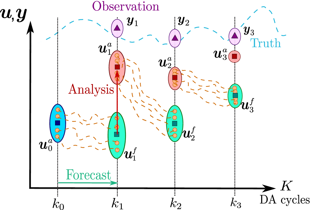
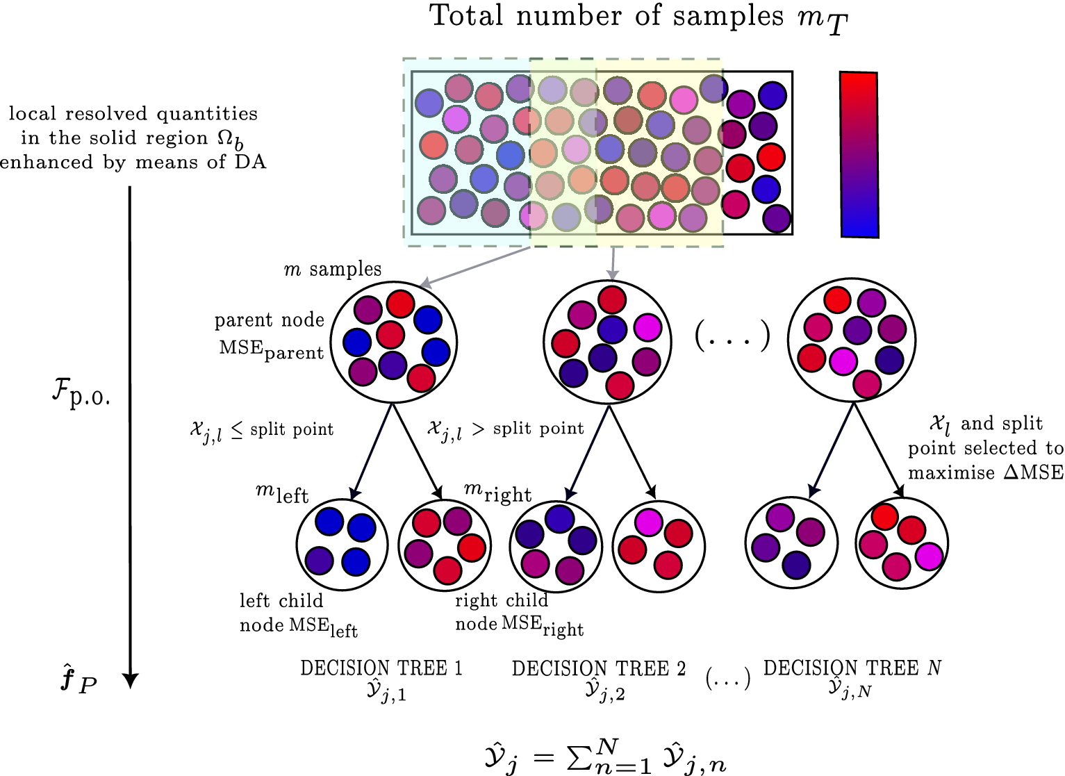
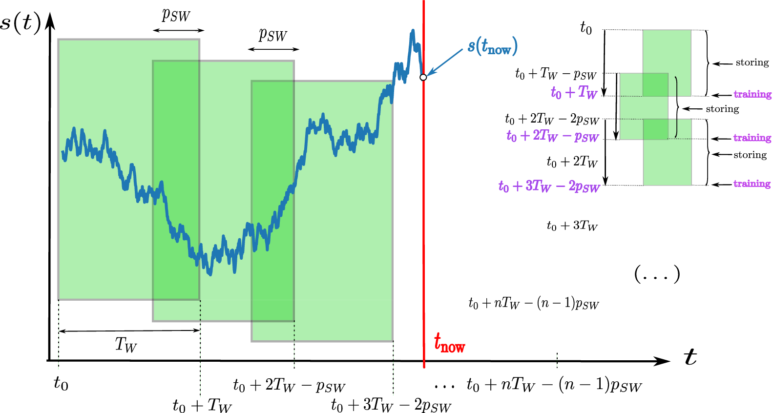


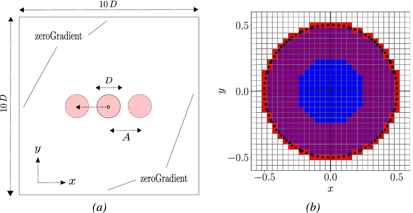

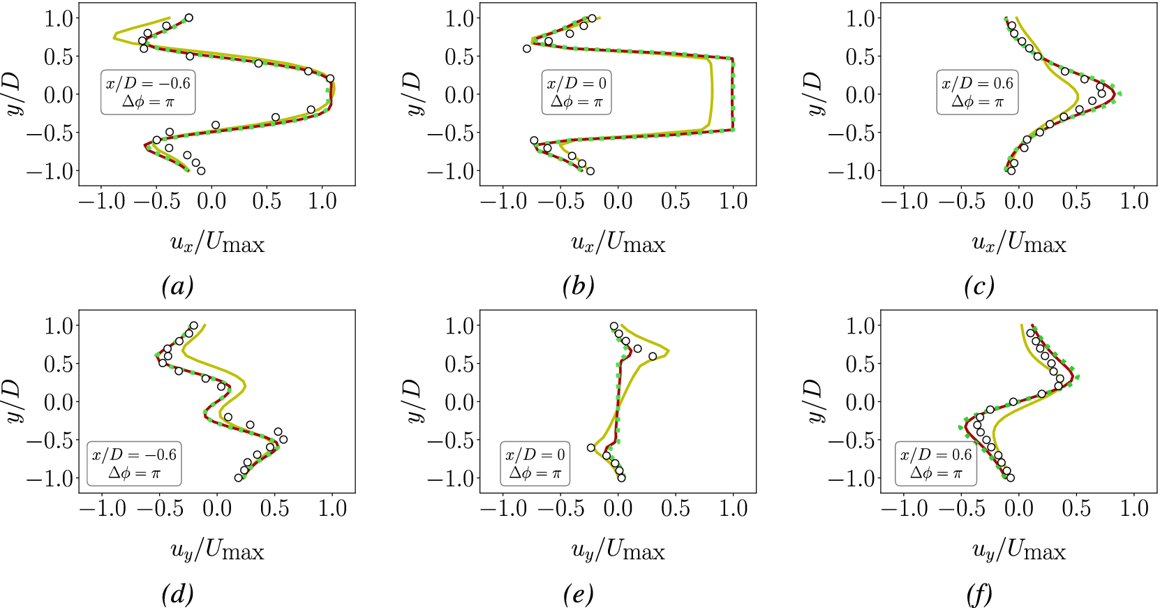


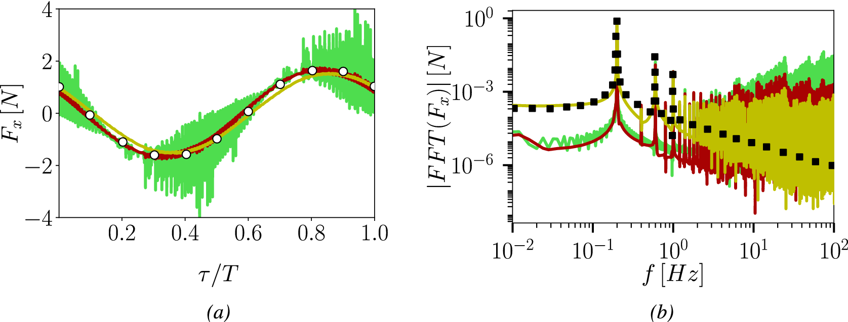


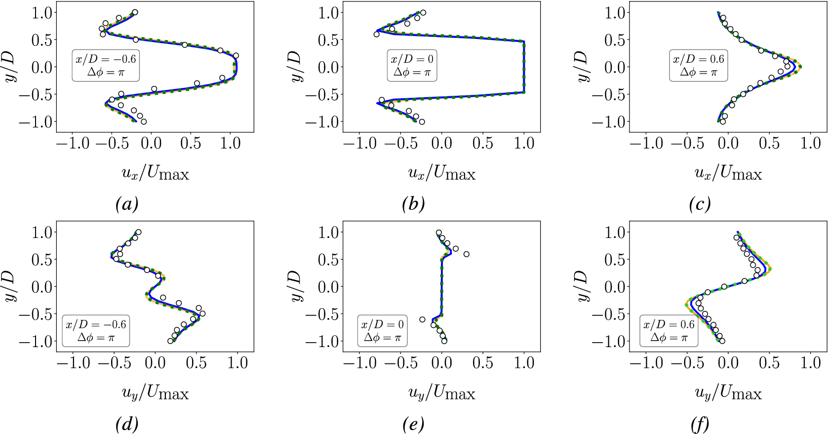


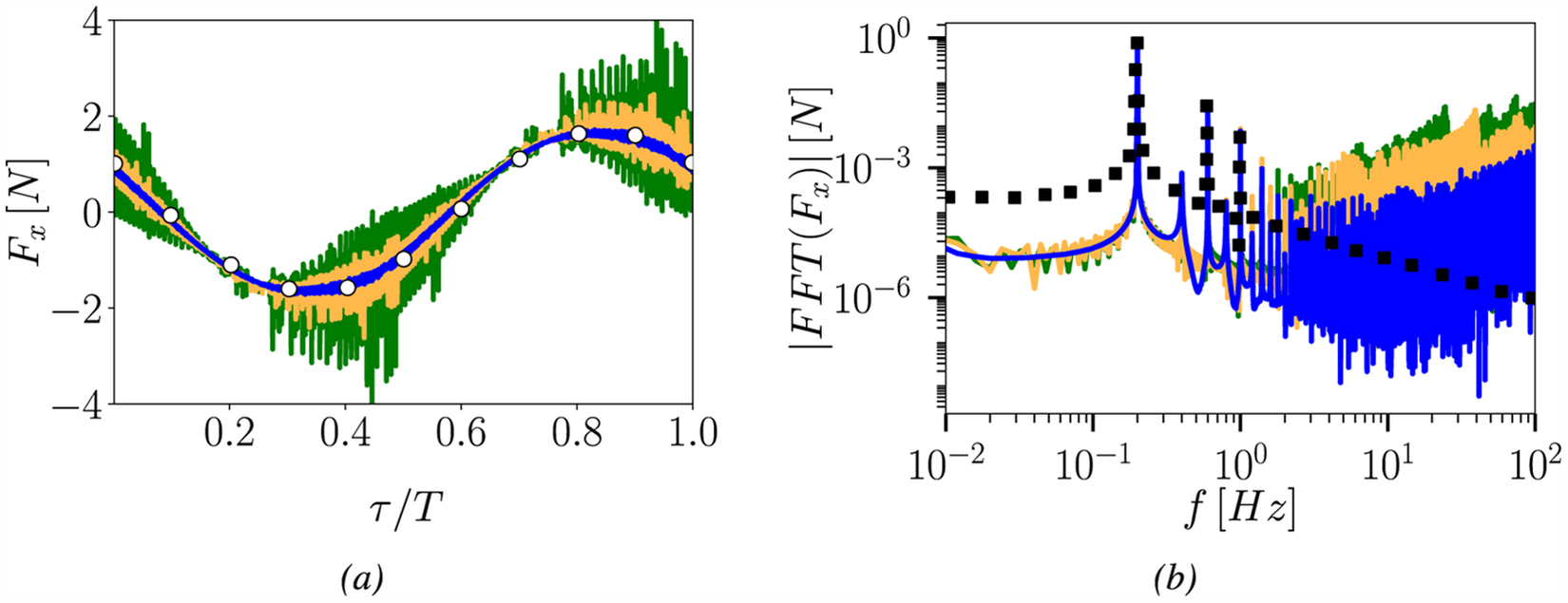


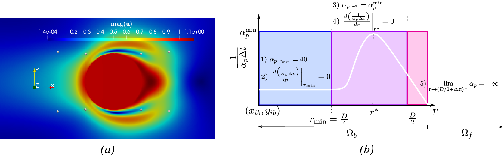


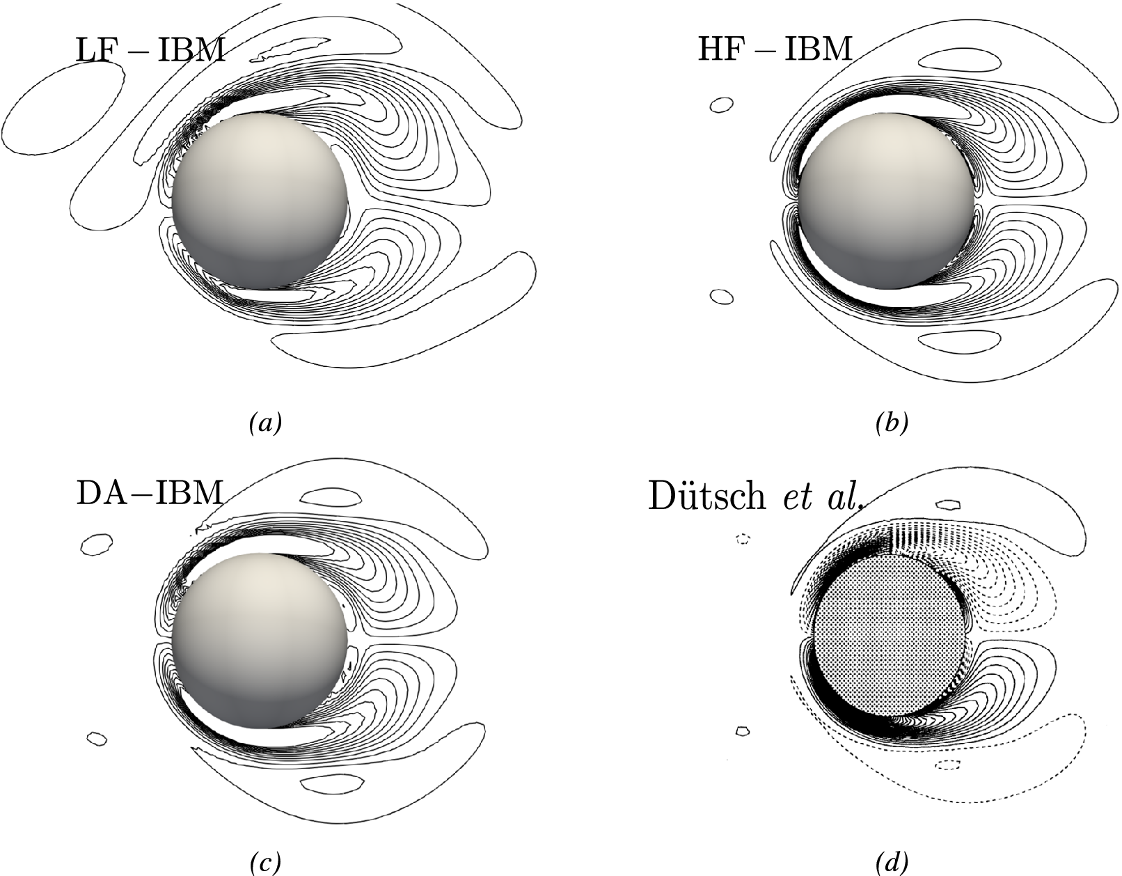


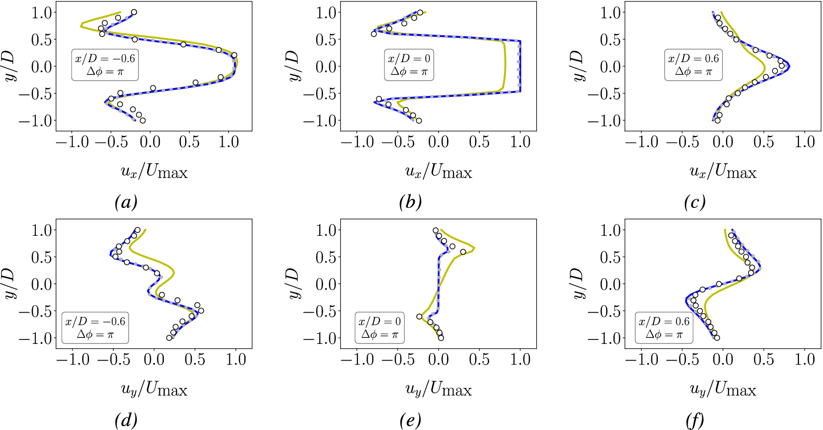


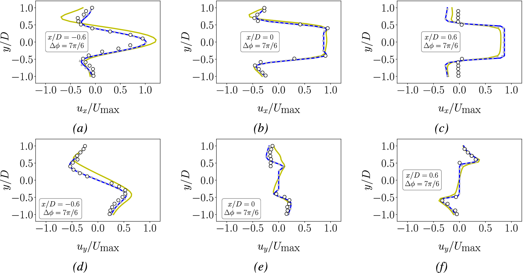


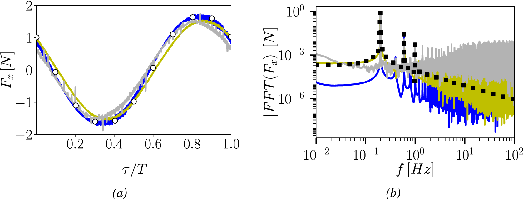



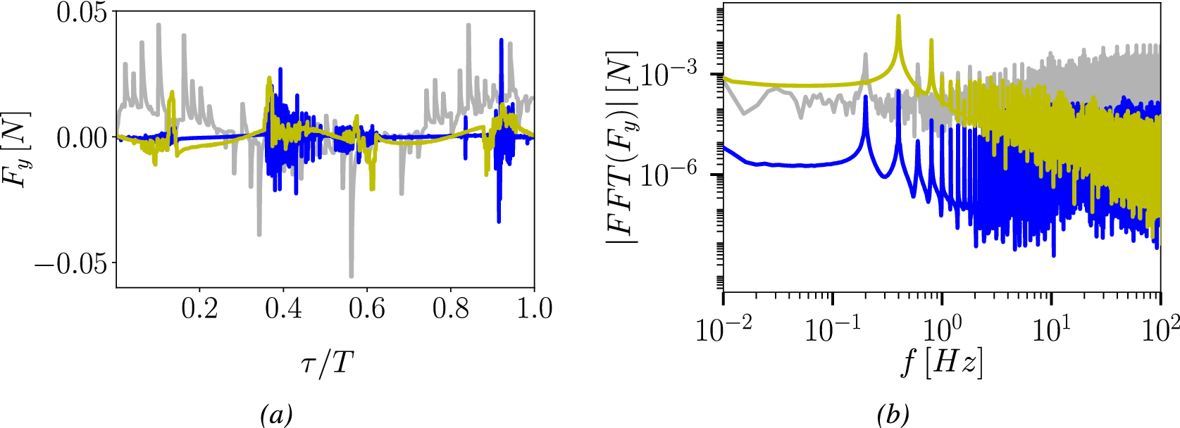


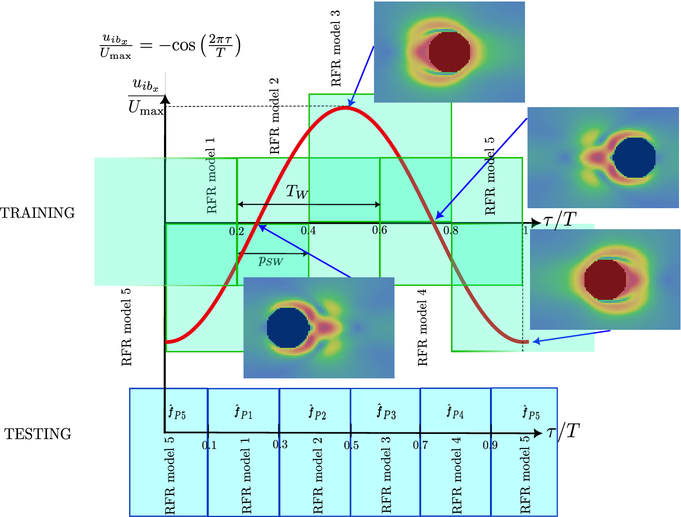

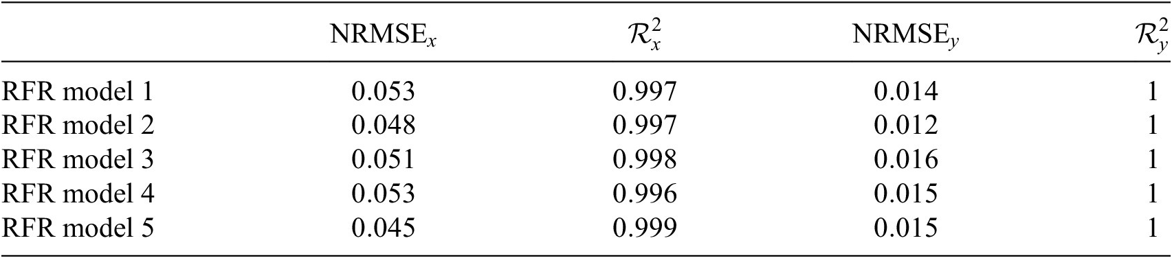


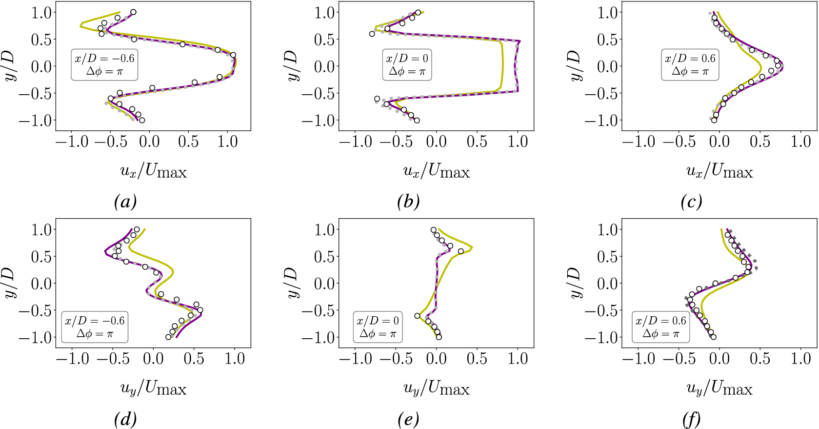


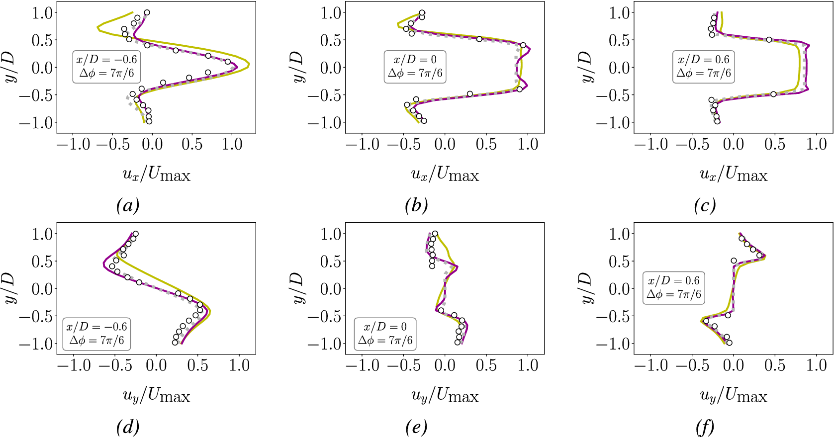


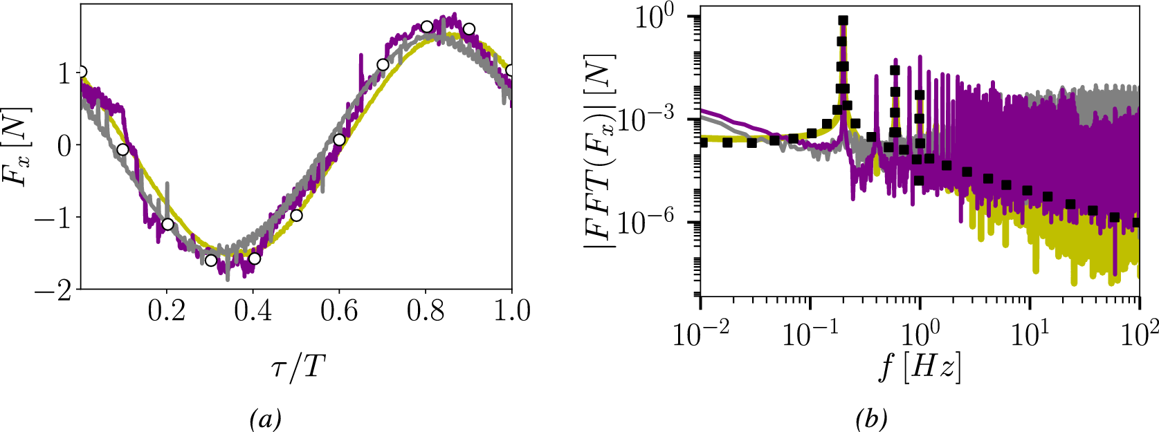


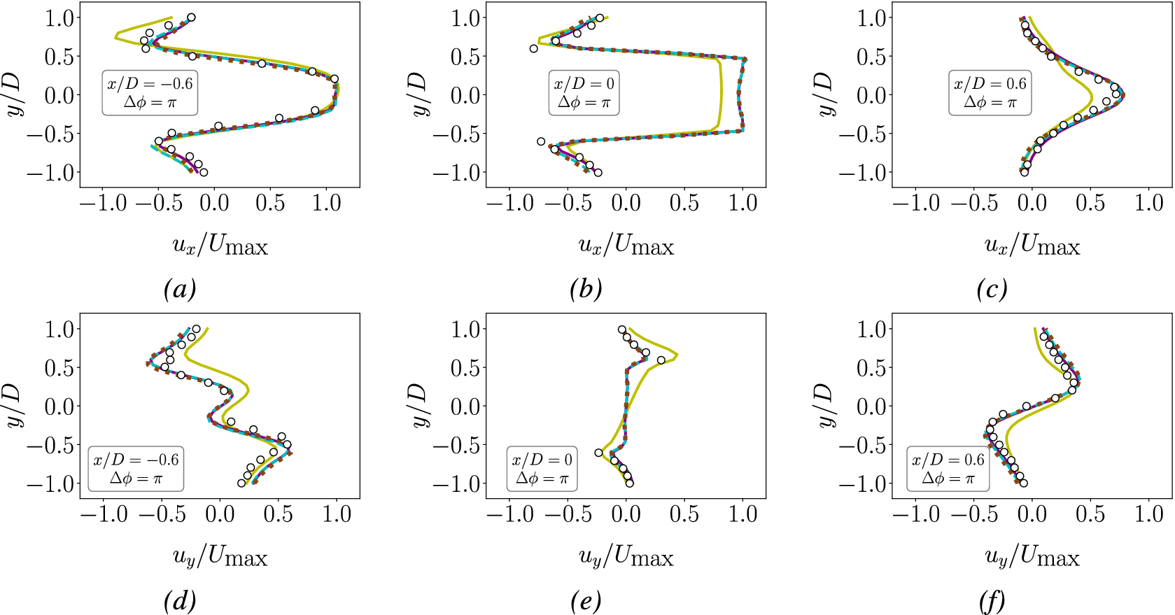


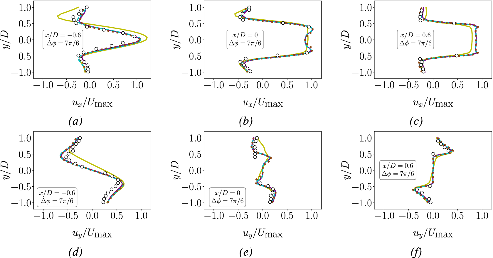


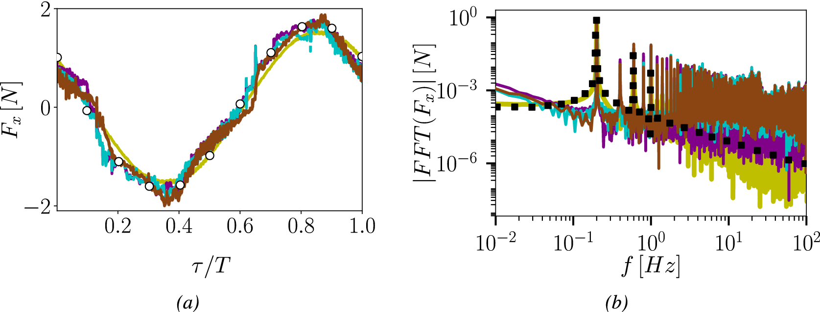


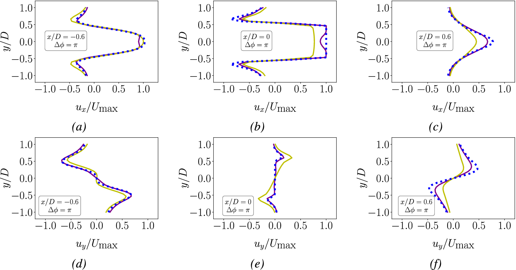


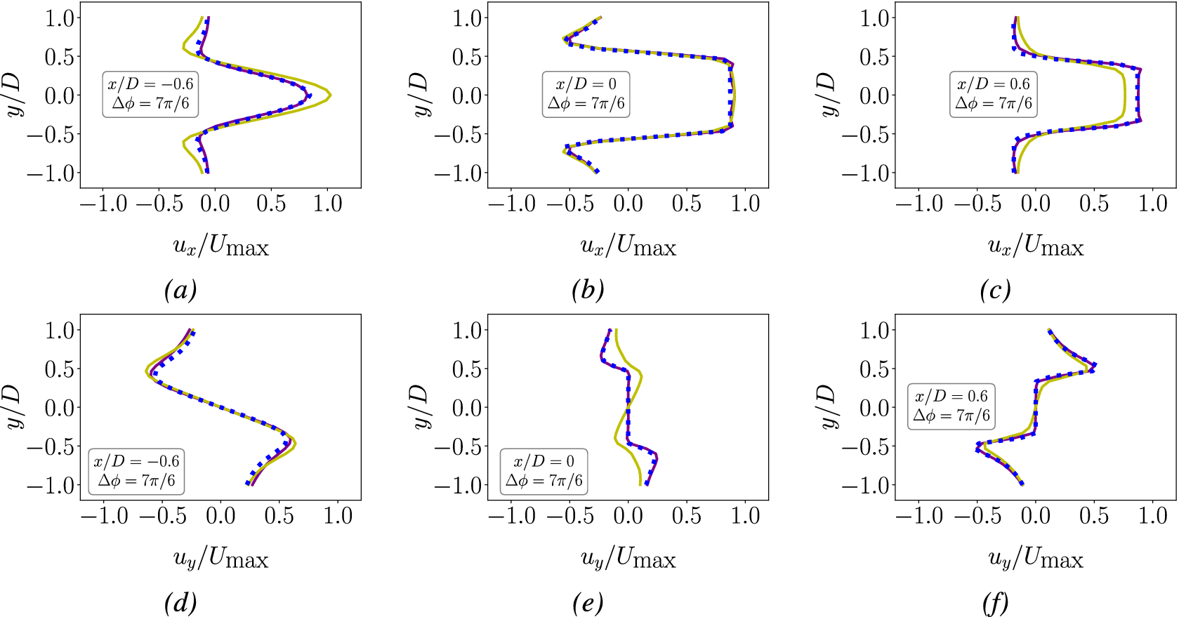


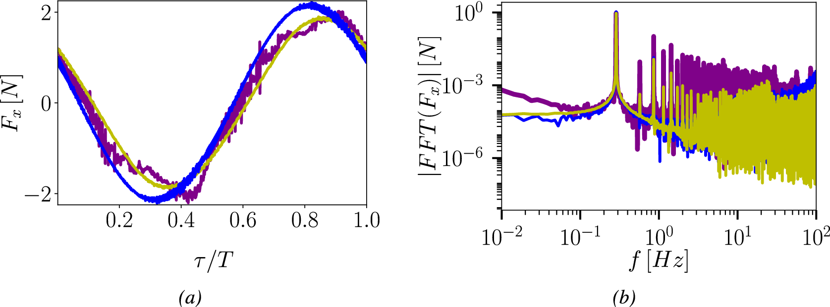


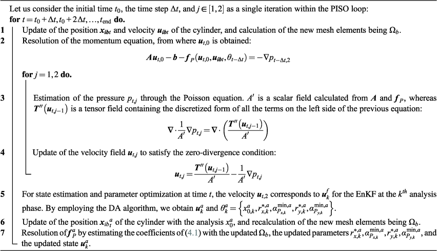
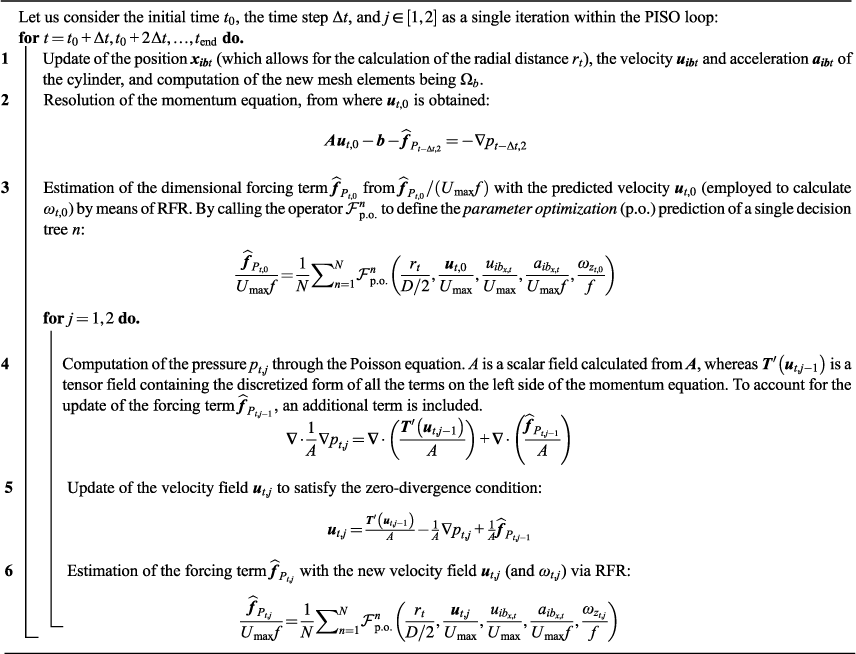

 Open access


Comments
No Comments have been published for this article.