2. Physical model

2.1. Kinetic model for partially ionised argon gas

2.1.1. General framework

We formulate the kinetic evolution of a partially ionised argon plasma using the coupled Boltzmann equations for neutral atoms ( $n$ ), ions ( $i$ ) and electrons ( $e$ )

(2.1) \begin{align} \frac {\partial f_n}{\partial t} + \boldsymbol{u} \boldsymbol{\cdot }\boldsymbol{\nabla} _{\!\boldsymbol{x}} f_n &= Q^{el}_{n} + Q^{ion}_{n}, \\[-12pt] \nonumber \end{align}

(2.2) \begin{align} \frac {\partial f_i}{\partial t} + \boldsymbol{u} \boldsymbol{\cdot }\boldsymbol{\nabla} _{\!\boldsymbol{x}} f_i + \frac {e\boldsymbol{E}}{m_i} \boldsymbol{\cdot }\boldsymbol{\nabla} _{\!\boldsymbol{u}} f_i &= Q^{el}_{i} + Q^{ion}_{i}, \\[-12pt] \nonumber \end{align}

(2.3) \begin{align} \frac {\partial f_e}{\partial t} + \boldsymbol{u} \boldsymbol{\cdot }\boldsymbol{\nabla} _{\!\boldsymbol{x}} f_e - \frac {e\boldsymbol{E}}{m_e} \boldsymbol{\cdot }\boldsymbol{\nabla} _{\!\boldsymbol{u}} f_e &= Q^{el}_{e} + Q^{ion}_e. \\[10pt] \nonumber \end{align}

Here, $f_s(\boldsymbol{x},\boldsymbol{u},t)$ denotes the velocity distribution function of species $s$ ( $s = n,i,e$ ); $\boldsymbol{x}$ and $\boldsymbol{u}$ are the position and microscopic velocity vectors, $t$ is time, $e$ is the elementary charge and $\boldsymbol{E}$ is the electric field. The right-hand side operators separate into elastic collisions ( $Q_s^{el}$ ) and the inelastic collisions of ionisation and recombination ( $Q_s^{ion}$ ).

When atoms and ions remain tightly coupled through frequent collisions, they share a common velocity and temperature distribution and can be merged into a single heavy-particle component. Defining the heavy-particle distribution function $f_h \equiv f_n + f_i$ , the degree of ionisation $\alpha \equiv n_i/(n_n+n_i)$ and the mean heavy-particle mass $m_h \equiv m_n \approx m_i$ (where $m_n$ and $m_i$ denote the neutral atom and ion masses, respectively), the kinetic equation for the heavy species reduces to

(2.4) \begin{align} \frac {\partial f_h}{\partial t} + \boldsymbol{u} \boldsymbol{\cdot }\boldsymbol{\nabla} _{\!\boldsymbol{x}} f_h + \alpha \frac {e\boldsymbol{E}}{m_h} \boldsymbol{\cdot }\boldsymbol{\nabla} _{\!\boldsymbol{u}} f_h = Q_{hh}^{\textit{el}}(f_h) + Q_{he}^{\textit{el}}(f_h, f_e) + Q^{ion}_n + Q^{ion}_i. \end{align}

Appendix A shows a detailed derivation of the above equation, where $Q_{hh}^{\textit{el}}(f_h), Q_{he}^{\textit{el}}(f_h, f_e)$ on the right-hand side describe elastic collisions among heavy particles and between heavy particles and electrons, respectively. Their detailed formulations are elaborated in the subsequent parts. The electrostatic force term acts only on ions, i.e. the fraction $\alpha$ of the heavy component and is therefore scaled by the local ionisation degree. Ambipolar diffusion is neglected in the present study, as ambipolar effects exert a negligible influence in the simulated flow conditions.

Regarding the description of electrons, we assume that electron–electron collisions are sufficiently frequent to maintain the electrons in local thermodynamic equilibrium, thereby justifying a fluid description. Under the quasi-neutrality condition $n_i \approx n_e$ , the electron continuity equation becomes redundant, as the electron number density is directly obtained from the ion density. The ion density itself is governed by the zeroth-order velocity moment of the ion kinetic equation, (2.2), which yields

(2.5) \begin{align} \frac {\partial \rho _i}{\partial t} + \boldsymbol{\nabla }\boldsymbol{\cdot }(\rho _i \boldsymbol{U}) = m_h \dot {n}_e, \end{align}

where $\rho _i = m_h n_i$ is the ion mass density and $\dot {n}_e$ denotes the volumetric production rate of electrons (and, by charge neutrality, of ions). The expression for $\dot {n}_e$ will be introduced in a subsequent section. Following the definition of the ionisation degree $\alpha = n_i / n$ , with $n = n_n + n_i$ the total heavy-particle number density, and writing the total heavy-particle mass density as $\rho = m_h n$ , the ion conservation equation transforms into

(2.6) \begin{align} \frac {\partial (\rho \alpha )}{\partial t} + \boldsymbol{\nabla }\boldsymbol{\cdot }(\rho \alpha \boldsymbol{U}) = m_h \dot {n}_e. \end{align}

Once $\alpha$ is known from this equation, the number densities of all species follow directly

(2.7) \begin{align} n_n = (1-\alpha )n, n_i = \alpha n, n_e = \alpha n. \end{align}

The macroscopic velocity of the electrons is assumed to be close to that of the heavy particles ( $\boldsymbol{U}_e \approx \boldsymbol{U}_h$ ), allowing the momentum slip and associated frictional drag between the two species to be neglected. Consequently, in the asymptotic limit of negligible electron mass ( $m_e \rightarrow 0$ ), the electron momentum equation reduces to a force balance between the electron pressure gradient and the self-consistent electrostatic field

(2.8) \begin{align} \boldsymbol{\nabla }p_e = -n_e e \boldsymbol{E}. \end{align}

Accordingly, the governing equation for the electron thermal energy is formulated as

(2.9) \begin{align} \rho _e c_{v,e}\left (\frac {\partial T_e}{\partial t} + \boldsymbol{U}_e\boldsymbol{\cdot }\boldsymbol{\nabla }T_e\right ) = \boldsymbol{\nabla }\boldsymbol{\cdot }(\kappa _e \boldsymbol{\nabla }T_e) - p_e(\boldsymbol{\nabla }\boldsymbol{\cdot }\boldsymbol{U}_e) + S_{eh} + S^{ion}_e, \end{align}

where the left-hand side represents the material derivative of the electron internal energy and $c_{v,e}= ({3}/{2})R_e$ is the constant-volume heat capacity of electrons. The right-hand side terms account for thermal conduction ( $\kappa_e$ denotes the electron thermal conductivity), compressive work, the energy exchange rate with the heavy-particle species ( $S_{eh}$ ) and the energy source term due to ionisation–recombination reactions ( $S^{ion}_e$ ), respectively.

By substituting the electron momentum balance equation (2.8) into the heavy-particle kinetic equation (2.4) and combining it with the degree of ionisation equation (2.6) and the electron energy transport model equation (2.9), the coupled kinetic-fluid governing system is established as follows:

(2.10) \begin{align} &\frac {\partial f_h}{\partial t} + \boldsymbol{u} \boldsymbol{\cdot }\boldsymbol{\nabla} _{\!\boldsymbol{x}} f_h -\frac {\boldsymbol{\nabla }p_e}{\rho _h} \boldsymbol{\cdot }\boldsymbol{\nabla} _{\!\boldsymbol{u}} f_h = Q_{hh}^{\textit{el}}(f_h) + Q_{he}^{\textit{el}}(f_h, f_e) + Q^{ion}_n + Q^{ion}_i , \\[-12pt] \nonumber \end{align}

(2.11) \begin{align} &\rho _e c_{v,e}\left (\frac {\partial T_e}{\partial t} + \boldsymbol{U}_e\boldsymbol{\cdot }\boldsymbol{\nabla }T_e\right ) = \boldsymbol{\nabla }\boldsymbol{\cdot }(\kappa _e \boldsymbol{\nabla }T_e) - p_e(\boldsymbol{\nabla }\boldsymbol{\cdot }\boldsymbol{U}_e) + S_{eh} + S^{ion}_e, \\[-12pt] \nonumber \end{align}

(2.12) \begin{align} &\frac {\partial (\rho \alpha )}{\partial t} + \boldsymbol{\nabla }\boldsymbol{\cdot }(\rho \alpha \boldsymbol{U}) = m_h \dot {n}_e . \\[10pt] \nonumber \end{align}

Further simplifications can be introduced to the above system. First, in the weakly ionised regime where $n_e \ll n_h$ , the electron pressure is negligible compared with the heavy-particle pressure ( $p_e \ll p_h$ ). Consequently, the electron pressure gradient term in (2.10) may be omitted. Second, following the widely adopted approximation for the electron energy equation (Petschek & Byron Reference Petschek and Byron1957; Morgan & Morrison Reference Morgan and Morrison1965; Hoffert & Lien Reference Hoffert and Lien1967), we retain only the dominant contributions from elastic energy exchange between electrons and heavy particles and from ionisation energy loss. The reduced governing system is expressed as

(2.13) \begin{align} &\frac {\partial f_h}{\partial t} + \boldsymbol{u} \boldsymbol{\cdot }\boldsymbol{\nabla} _{\!\boldsymbol{x}} f_h = Q_{hh}^{\textit{el}}(f_h) + Q_{he}^{\textit{el}}(f_h, f_e) + Q^{ion}_n + Q^{ion}_i , \\[-12pt] \nonumber \end{align}

(2.14) \begin{align} &\rho _e c_{v,e}\frac {\partial T_e}{\partial t} = S_{eh} + S^{ion}_e, \\[-12pt] \nonumber \end{align}

(2.15) \begin{align} &\frac {\partial (\rho \alpha )}{\partial t} + \boldsymbol{\nabla }\boldsymbol{\cdot }(\rho \alpha \boldsymbol{U}) = m_h \dot {n}_e . \\[10pt] \nonumber \end{align}

2.1.2. Elastic collision operators

Next, the explicit formulations of the collision operators are detailed. The heavy-particle elastic collision operator, $Q^{\textit{el}}_{hh}$ , is modelled using the Bhatnagar–Gross–Krook (BGK) relaxation approximation

(2.16) \begin{align} Q^{\textit{el}}_{hh} = \frac {g_h - f_h}{\tau _h}, \end{align}

where $g_h$ denotes the local Maxwellian equilibrium distribution function, defined as

(2.17) \begin{align} g_h = \rho _h \left ( \frac {m_h}{2 \pi k_B T_h} \right )^{3/2} \exp \left [ -\frac {m_h}{2 k_B T_h} (\boldsymbol{u} - \boldsymbol{U}_h)^2 \right ]. \end{align}

Here, $\rho _h$ , $\boldsymbol{U}_h$ and $T_h$ represent the total mass density, macroscopic bulk velocity and temperature of the heavy-particle mixture, respectively, and $k_B$ is the Boltzmann constant. The characteristic relaxation time $\tau _h$ is calculated as $\tau _h = 1/(1/\tau _{hh}+1/\tau _{he})$ , where $\tau _{hh}$ is the mean collision time between heavy particles and $\tau _{he}$ is the mean collision time between heavy particles and electrons. In the weakly ionised regime ( $\alpha \ll 1$ ), the collision model of the atom–ion mixture is approximated by that of pure neutral atoms. Specifically, $\tau _{hh}=1/(\chi _{hh}n_h)$ , and the interaction coefficient $\chi _{hh}$ is

(2.18) \begin{align} \chi _{hh}= \frac {(5-2\omega )(7-2\omega )\sqrt { \pi }}{15}\left (\frac {4 k_B T_{h}}{m_h}\right )^{1 / 2}d_h^2, \end{align}

where $ d_h$ represents the diameters of the heavy particles. The temperature modifies the molecular diameter as $ ({d}/{d_{ref}})^2 = ( {T}/{T_{ref}} )^{({1}/{2}) - \omega },$ where $\omega$ is the power coefficient between viscosity and temperature (Bird Reference Bird1994); $\omega =0.81$ is used for argon atoms, $\tau _{he}=\tau _{eh}/ \alpha =1/(\nu _{eh}\alpha)$ and $\nu _{eh}$ is detailed in the subsequent part in this section.

The collision term $Q_{he}^{el}$ denotes cross-species collision between electrons and heavy particles and is denoted as

(2.19) \begin{align} Q_{he}^{el} = \frac {g^M - g_h}{\tau _{h}}, \end{align}

where $g^M$ denotes the local Maxwell distribution after the collision with electrons, which reads

(2.20) \begin{align} g^M = \rho _h \left ( \frac {m_h}{2 \pi k_B \bar {T}_h} \right )^{3/2} \exp \left [ -\frac {m_h}{2 k_B \bar {T}_h} (\boldsymbol{u} - \boldsymbol{\bar {U}}_h)^2 \right ] . \end{align}

The post-collision temperature $\bar {T}_h$ is given as

(2.21) \begin{align} \bar {T}_h =T_h+\tau _h \frac {4 m_{h e} \sigma _{s,he} v_{th,e} n_e}{m_h+m_e}\left (T_e-T_h\right ), \end{align}

where the reduced mass is $m_{he} = ({m_hm_e})/({m_h + m_e})$ , and $\sigma _{s,he}$ denotes the collision cross-section of heavy particles and electrons, $v_{th,e}$ is the mean thermal speed of electrons. Under the assumption that electrons and heavy particles move with the same velocity, the cross-species post-collision velocity remains invariant, yielding $\boldsymbol{\bar {U}}_h = \boldsymbol{U}_h$ .

The energy exchange term $S_{eh}^{el}$ in (2.9) accounts for elastic collisional transfer of thermal energy between electrons and heavy particles. The exchange rate can be derived from the elastic collision integral and is given by

(2.22) \begin{align} S_{eh}^{el} = 6n_e \frac {m_e}{m_h} \nu _{eh} k_B (T_h - T_e), \end{align}

where $\nu _{eh}$ and $\nu _{ei}$ are the electron and heavy-particle collision frequencies. The collision frequency is computed as

(2.23) \begin{align} \nu _{eh} = \nu _{en} + \nu _{ei} = n_n \sigma _{s,en} v_{\textit{th},e} + n_i \sigma _{s,ei} v_{\textit{th},e}, \end{align}

with $\sigma _{s,en}$ and $\sigma _{s,ei}$ the electron–atom and electron–ion momentum-transfer scattering cross-section, respectively, and $ v_{\textit{th},e} = \sqrt {8 k_B T_e/(\pi m_e)}$ . For the electron–atom cross-section, we use the piecewise fit by Jaffrin (Reference Jaffrin1965)

(2.24) \begin{align} \sigma _{\textit{s,en}} = \left \{ \begin{array}{ll} \big( -0.35 + 0.775 \times 10^{-4} T_{e} \big) \times 10^{-20} \,\text{m}^{2} \, & T_{e} \geq 10^4 \, \mathrm{K}, \\[10pt] \begin{array}{l} \big( 0.39 - 0.551 \times 10^{-4} T_{e} + 0.595 \times 10^{-8} T_{e}^2 \big) \times 10^{-20} \,\text{m}^{2}\, \end{array} & T_{e} \lt 10^4 \, \mathrm{K}. \end{array} \right . \end{align}

For the electron–ion cross-section (Sutton & Sherman Reference Sutton and Sherman2006)

(2.25) \begin{align} \begin{aligned} \sigma _{s,ei} & =\frac {2 \pi e^4}{9 k_B^2 T_e^2} \ln \left (\frac {9 k_B^3 T_e^3}{4 \pi e^6 n_{e}}\right ) =1.95 \times 10^{-10} T_e^{-2.0} \ln \left (1.53 \times 10^8 \frac {T_e^3}{n_{e}}\right ) \,\text{m}^{2} \end{aligned}\!. \end{align}

The thermal conductivity of electrons $\kappa _e = ({5}/{2}) R_e p_e \tau _e$ , where $R_e =k_B/m_e$ is the specific gas constant for electrons and $\tau _e$ is the electron mean relaxation time given as

(2.26) \begin{align} \tau _e = \frac {1}{\nu _{ee} + \nu _{eh}}, \end{align}

where the electron–electron collision frequency is given by (Braginskii Reference Braginskii1965; Angus et al. Reference Angus, Dun, Farmer, Geyko, Grote, Larson, van de, Johannes and Zimmerman2025)

(2.27) \begin{align} \nu _{ee} = \frac {n_e \ln \varLambda _{ee}}{2.7518\times 10^5 T_e^{3/2}} , \end{align}

where $\ln \varLambda _{ee}=10$ is the Coulomb logarithm.

2.1.3. Inelastic collision operators

We now introduce the treatment of inelastic collision operators. The ionisation model adopted in this study comprises thermal ionisation (TI) and electron-impact ionisation (EI) (Hoffert & Lien Reference Hoffert and Lien1967)

(2.28) \begin{align} \begin{aligned}\textit{TI}&:\quad {Ar} + {Ar} \rightleftharpoons {Ar}^+ + e^- + {Ar},\\ \textit{EI}&:\quad {Ar} + e^- \rightleftharpoons {Ar}^+ + e^- + e^-. \end{aligned} \end{align}

The forward rate coefficients are

(2.29) \begin{align} \begin{aligned} k_{f{\kern-0.5pt}A}(T_h) &= 1.68 \times 10^{-26}\; T_h^{1.5} \left ( \frac {\varTheta _{A,1}^*}{T_h} + 2 \right ) \exp \!\left (-\frac {\varTheta _{A,1}^*}{T_h}\right )\!,\\[5pt] k_{fe}(T_e) &= 3.75 \times 10^{-22}\; T_e^{1.5} \left ( \frac {\varTheta _{A,1}^*}{T_e} + 2 \right ) \exp \!\left (-\frac {\varTheta _{A,1}^*}{T_e}\right )\!, \end{aligned} \end{align}

and the backward (recombination) rate coefficients are

(2.30) \begin{align} \begin{aligned} k_{\textit{rA}}(T_h) &= 5.80 \times 10^{-49} \left ( \frac {\varTheta _{A,1}^*}{T_h} + 2 \right ) \exp \!\left ( \frac {\varTheta _{\textit{ion}} - \varTheta _{A,1}^*}{T_h} \right )\!,\\[5pt] k_{re}(T_e) &= 1.29 \times 10^{-44} \left ( \frac {\varTheta _{A,1}^*}{T_e} + 2 \right ) \exp \!\left ( \frac {\varTheta _{\textit{ion}} - \varTheta _{A,1}^*}{T_e} \right )\!. \end{aligned} \end{align}

Here, $\varTheta _{A,1}^* = \epsilon _{A,1}^* / k_B = 135\,300\ \text{K}$ is the characteristic temperature of the first excited state of argon, with $\epsilon _{A,1}^*$ the characteristic energy, and $\varTheta _{\textit{ion}} = \epsilon _{\textit{ion}} / k_B = 183\,100\ \text{K}$ is the characteristic temperature for first ionisation, with $\epsilon _{\textit{ion}}$ the characteristic energy also. Unlike the conventional Arrhenius form, these expressions follow from the assumption that the inelastic cross-section varies linearly with the collisional kinetic energy (Hoffert & Lien Reference Hoffert and Lien1967), which produces the additional factor $\varTheta _{A,1}^*/T + 2$ . The forward and reverse reaction rates satisfy the principle of detailed balance, naturally recovering the expected Saha equilibrium limit.

Rather than evaluating the full Boltzmann collision integrals for ionisation and recombination, we treat these inelastic processes through their velocity moments, which supply the necessary source terms for the macroscopic fluid equations. For the heavy species, the zeroth-order moment of the inelastic operators vanishes because the total number of heavy particles is conserved during ionisation and recombination

(2.31) \begin{align} \int m_h \big(Q_n^{\textit{ion}} + Q_i^{\textit{ion}}\big)\, \mathrm d\boldsymbol{u} = 0. \end{align}

The second-order moment gives the net energy exchange rate of the heavy particles with the ionisation process

(2.32) \begin{align} \int \frac {1}{2} m_h |\boldsymbol{u}|^2 \big(Q_n^{\textit{ion}} + Q_i^{\textit{ion}}\big)\, \mathrm d\boldsymbol{u} = S_h^{\textit{ion}}, \end{align}

where $S_h^{\textit{ion}}$ represents the energy source term associated with TI. It is modelled as

(2.33) \begin{align} S_h^{\textit{ion}} = -\epsilon _{\textit{ion}} \,[\dot {n}_e]_{\textit{TI}}, \end{align}

with $[\dot {n}_e]_{\textit{TI}}$ denoting the net electron production rate by atom–atom collisions. For electrons, the corresponding energy loss due to EI is

(2.34) \begin{align} S_e^{\textit{ion}} = -\epsilon _{\textit{ion}} \,[\dot {n}_e]_{\textit{EI}}, \end{align}

where $[\dot {n}_e]_{\textit{EI}}$ is the net electron production rate by electron-impact collisions. The ionisation energy source terms $S_h^{\textit{ion}}$ and $S_e^{\textit{ion}}$ enter the heavy-particle and electron energy equations, respectively. The coupling between these macroscopic source terms and the microscopic distribution function is detailed in the numerical methods section.

The net electron production rate from each channel is expressed in terms of the number densities as

(2.35) \begin{align} [\dot {n}_e]_{\textit{TI}} &= k_{f{\kern-0.5pt}A} n_n^2 - k_{rA} n_i n_e n_n,\nonumber \\[5pt] [\dot {n}_e]_{\textit{EI}} &= k_{fe} n_n n_e - k_{re} n_i n_e^2. \end{align}

The total electron production rate $\dot {n}_e = [\dot {n}_e]_{\textit{TI}} + [\dot {n}_e]_{\textit{EI}}$ is given by substituting relation (2.7) into the above formula

(2.36) \begin{align} \dot {n}_e = n^2 (1-\alpha ) \bigl [ k_{f{\kern-0.5pt}A}(1-\alpha ) + k_{fe}\alpha \bigr ] \;-\; n^3 \alpha ^2 \bigl [ k_{rA}(1-\alpha ) + k_{re}\alpha \bigr ]. \end{align}

This expression directly provides the source term $S = m_h \dot {n}_e$ required in the ionisation-degree equation (2.6).

2.2. Auxiliary differential equation for plasma medium

We model the plasma’s response to the electromagnetic field using an auxiliary differential equation (ADE) (Sun et al. Reference Sun, Wang, Han, Cui, Sun, Shi and Zhao2018). The current density equation capturing plasma oscillation and collisional effects is

(2.37) \begin{align} \frac {\partial \boldsymbol{J}}{\partial t} + \nu _{eh}\boldsymbol{J} = \epsilon _{0}\omega _{p}^2\boldsymbol{E}, \end{align}

where $\boldsymbol{J}$ is the current density and $\nu _{eh}$ the electron collision frequency with heavy particles, as introduced in the previous section. The plasma frequency $\omega _p = \sqrt {n_e e^2/m_e \epsilon _0}$ , and $\epsilon _0$ is the vacuum permittivity.

3. Numerical method

3.1. General procedure

The overall simulation comprises two modules. The first module solves the hybrid kinetic-fluid reactive gas dynamics and supplies the electron number density $n_e$ and temperature $T_e$ to the second module. The second module computes the electromagnetic-wave propagation and plasma dispersion. The complete workflow is depicted in figure 1.

Figure 1.

Flowchart of the hybrid kinetic-fluid and electromagnetic simulation framework. Stage 1 resolves the thermochemical non-equilibrium gas dynamics: the heavy-particle transport is handled by the multiscale UGKWP method from the rarefied to the continuum regime, and the electron temperature is advanced macroscopically. The electron number density $n_e$ and temperature $T_e$ are then passed to stage 2, where electromagnetic-wave propagation and the plasma response are simulated using a Maxwell solver and the current density ADE formulation, respectively.

The time integration of the thermochemical non-equilibrium flow in the first module employs an operator-splitting procedure. Within each time step $\Delta t = t^{n+1} - t^n$ , the following substeps are executed sequentially.

Step 1: heavy-particle transport. The heavy-particle transport is handled by the multiscale UGKWP method from the rarefied to the continuum regime

(3.1) \begin{align} \boldsymbol{W}_h^* = \mathcal{L}_1^{fl} \big(\boldsymbol{W}_h^n \big), \end{align}

where $\mathcal{L}_1^{fl}$ denotes the UGKWP algorithm.

Step 2: chemical reactions and two-temperature coupling. The ionisation kinetics and the accompanying energy exchange are integrated locally

(3.2) \begin{align} \big(\alpha ^{n+1}, T_h^{**}, T_e^{**} \big) = \mathcal{L}_2^{fl} \big(\alpha ^*, T_h^*, T_e^* \big). \end{align}

The updated temperatures and ionisation fraction are then mapped back to the conservative variables through

(3.3) \begin{align} \boldsymbol{W}^{**} = \mathcal{H}(\boldsymbol{W}^*), \end{align}

where $\mathcal{H}$ enforces consistency between primitive and conservative states.

Step 3: elastic energy relaxation. The electron–heavy-particle thermal relaxation is applied

(3.4) \begin{align} \big(T_h^{n+1}, T_e^{n+1} \big) = \mathcal{L}_3^{fl} \big(T_h^{**}, T_e^{**} \big). \end{align}

A final conservative projection, $\boldsymbol{W}^{n+1} = \mathcal{H}(\boldsymbol{W}^{**})$ , completes the time advancement of the gas-dynamics module.

The electromagnetic module advances in two steps.

Step 1: electromagnetic-wave propagation. The source-free Maxwell equations are solved using a GKS scheme (Pu et al. Reference Pu, Long and Xu2024b ) to propagate the electromagnetic fields

(3.5) \begin{align} \boldsymbol{Q}^* = \mathcal{L}_1^{em}(\boldsymbol{Q}^n), \end{align}

where $\boldsymbol{Q} = (\boldsymbol{E}, \boldsymbol{B})$ denotes the macroscopic electromagnetic variables.

Step 2: plasma wave dispersion. The ADE for the current density is coupled implicitly with Ampere’s law to evolve the current density and the electric field concurrently

(3.6) \begin{align} \boldsymbol{Q}^{n+1} = \mathcal{L}_2^{em}(\boldsymbol{Q}^*). \end{align}

3.2. The UGKWP method for coupled transport and collision step

First, we introduce algorithms for solving $\mathcal{L}_1^{fl}$ , where $\mathcal{L}_1^{fl}$ describes kinetic transport and collision. We solve it using the UGKWP method, which removes the time step restriction imposed by the mean collision time in the near-continuum regime. The core idea of the UGKWP method is to couple the evolution of collision and free transport rather than treating them in a split manner as in purely particle methods such as the DSMC method (Zhu et al. Reference Zhu, Liu, Zhong and Xu2019; Liu et al. Reference Liu, Zhu and Xu2020). In the framework of the finite volume method (FVM), the time-dependent solution of the distribution function at a cell interface can be written as

(3.7) \begin{align} f\left (\boldsymbol{x},\boldsymbol{u}, t\right )=\frac {1}{\tau } \int _{0}^{t} g(\boldsymbol{x}^{\prime }, \boldsymbol{u}, t^{\prime }) e^{-\left (t-t^{\prime }\right ) / \tau } \mathrm{d} t^{\prime } + e^{-t / \tau } f_{0}\left (\boldsymbol{x}-\boldsymbol{u} t \right ), \end{align}

where $\tau$ is the local mean relaxation time, $f_0$ is the initial gas distribution function at $t=0$ and $g$ is the equilibrium distribution along the characteristic line $\boldsymbol{x}^{\prime } = \boldsymbol{x} - \boldsymbol{u} t^{\prime }$ . The equation implies that a particle has a probability of $e^{-t/\tau }$ to freely stream during the time interval $[0,t]$ , and a probability of $(1 - e^{-t/\tau })$ to collide with other particles.

Based on this physical picture, the UGKWP method represents the velocity distribution function in a wave–particle coupled manner. For particles that experience collisions (the fraction $1 - e^{-t/\tau }$ ), we assume they enter a near-equilibrium distribution. Their contribution to the numerical flux is captured analytically through the equilibrium distribution $g$ , which is determined from the macroscopic variables. The remaining collisionless particles are represented by stochastic simulation particles $P_k (m_k, \boldsymbol{x}_k, \boldsymbol{u}_k)$ . Here, $m_k$ is the mass of a simulation particle $P_k$ , corresponding to a cluster of real gas particles; $\boldsymbol{x}_k$ and $\boldsymbol{u}_k$ are its position and velocity, respectively. This approach removes the constraints that require the time step and mesh size to be smaller than the mean collision time and the mean free path.

In the procedure above, we require the exact macroscopic variables to determine the local equilibrium distribution. In the FVM framework, the cell-averaged macroscopic conservative variables on a physical cell $\varOmega _i$ are updated by the numerical flux through cell interfaces

(3.8) \begin{align} (\boldsymbol{W} )_i^{*} = (\boldsymbol{W} )_i^n - \frac {\Delta t}{|\varOmega _i|}\sum _{s\in \partial \varOmega _i}|l_s|( {F}_{\boldsymbol{W} })_s, \end{align}

where $l_s\in \partial \varOmega _i$ is the cell interface with centre $\boldsymbol{x}_s$ and outer unit normal vector $\boldsymbol{n}_{s}$ and $|l_s|$ is the area of the cell interface. The numerical flux across the interface $( {F}_{\boldsymbol{W} })_s$ can be evaluated from distribution function at the interface

(3.9) \begin{align} ( {F}_{\boldsymbol{W} })_s = \frac {1}{\Delta t}\int _{t^n}^{t^{n+1}}\boldsymbol{u}\boldsymbol{\cdot }\boldsymbol{n}_sf (\boldsymbol{x}_{s},\boldsymbol{u},t)\boldsymbol{\varPsi } \mathrm{d}\boldsymbol{u}\mathrm{d}t, \end{align}

where $\boldsymbol{\varPsi }=(1,\boldsymbol{u}, ({1}/{2})|\boldsymbol{u}|^2)$ is the conservative moments of distribution functions. For the cell interface $l_s$ , the distribution function $f (\boldsymbol{x}_{s},\boldsymbol{u},t)$ requires direct tracking of its evolution in a wave–particle manner as introduced previously. This numerical flux of the macroscopic conservative variable can be split into the equilibrium flux and free-streaming flux according to (3.7). The equilibrium flux is

(3.10) \begin{align} ( {F}_{\boldsymbol{W}})_s^g = \frac {1}{\Delta t}\int _{}^{}\boldsymbol{u} \boldsymbol{\cdot }\boldsymbol{n}_{s}\left ( C_{1}g_{0} + C_{2}\boldsymbol{u} \boldsymbol{\cdot }{\boldsymbol{g}}_{0x} + C_{3}g_{0t} \right )\boldsymbol{\varPsi } \mathrm d\boldsymbol{u}, \end{align}

where $g_0$ is the equilibrium distribution function on the cell interface, $g_{0x}, g_{0t}$ are the spatial and temporal slopes of $g_0$ . Detailed derivations of these terms can be found in Pu & Xu (Reference Pu and Xu2025). The time integration coefficients are

(3.11) \begin{align} &C_{1} = \Delta t - \tau \big ( 1 - e^{- \Delta t\text{/}\tau } \big ) ,\nonumber \\&C_{2} = 2\tau ^2 \big(1 - e^{- \Delta t\text{/}\tau } \big) - \tau \Delta t -\tau \Delta t e^{- \Delta t\text{/}\tau },\nonumber \\&C_{3} = \frac {\Delta t^2}{2} - \tau \Delta t + \tau ^2 \big(1-e^{-\Delta t/\tau } \big). \end{align}

The analytical free-streaming flux $( {F}_{\boldsymbol{W}})_s^{f,w}$ contributed from the collisional particles is given as

(3.12) \begin{align} ( {F}_{\boldsymbol{W}})_s^{f,w} = \frac {1}{\Delta t}\int _{}^{}\boldsymbol{u} \boldsymbol{\cdot }\boldsymbol{n}_s\left ( C_{4}g_{0}^{h} + C_{5}\boldsymbol{u} \boldsymbol{\cdot }{g}_{0x}^{h} \right )\boldsymbol{\varPsi }\mathrm d\boldsymbol{u}, \end{align}

where $g_0^h$ denotes the equilibrium distribution function of the wave component. The macroscopic wave contribution is defined as $\boldsymbol{W}^h = \boldsymbol{W} - \boldsymbol{W}^p$ , where $\boldsymbol{W}^p$ represents the macroscopic conservative variables of the particle component and $g_{0x}^h$ is the spatial slope of $g_0^h$ . The time integration coefficients are

(3.13) \begin{align} &C_{4} = \tau \big ( 1 - e^{- \Delta t\text{/}\tau } \big ) - \Delta te^{- \Delta t\text{/}\tau } ,\nonumber \\[3pt]&C_{5} = \tau \Delta t e^{- \Delta t\text{/}\tau } - \tau ^{2}\big ( 1 - e^{- \Delta t\text{/}\tau } \big ) + \frac {\Delta t^{2}}{2}e^{- \Delta t\text{/}\tau }. \end{align}

The net particle flux $( {F}_{\boldsymbol{W}})_s^{f,p}$ is calculated as

(3.14) \begin{align} ( {F}_{\boldsymbol{W}})_s^{f,p}= \sum _{k \in P_{\partial \varOmega _{i}^{+}}}^{}\boldsymbol{W}_{P_{k}} - \sum _{k \in P_{\partial \varOmega _{i}^{-}}}^{}\boldsymbol{W}_{P_{k}}, \end{align}

where $\boldsymbol{W}_{P_{k}} = ( m_{k},m_{k}\boldsymbol{v}_{k},({1}/{2})m_{k}\boldsymbol{v}_{\boldsymbol{k,}}^{2} ),P_{\partial \varOmega _{i}^{-}}$ is the index set of the particles streaming out of cell $\varOmega _{i}$ during a time step and $P_{\partial \varOmega _{i}^{+}}$ is the index set of the particles streaming into cell $\varOmega _{i}$ . Finally, the update formula for conservative variables is

(3.15) \begin{align} \boldsymbol{W}_{i}^{*} = \boldsymbol{W}_{i}^{n} - \sum _{s}^{}{\frac {\Delta t}{\left | \varOmega _{i} \right |}\left | l_{s} \right |( {F}_{\boldsymbol{W}})_s^{g}} -\sum _{s}^{}{\frac {\Delta t}{\left | \varOmega _{i} \right |}\left | l_{s} \right |( {F}_{\boldsymbol{W}})_s^{f,w}} + \frac {1}{\left | \varOmega _{i} \right |}( {F}_{\boldsymbol{W}})_s^{f,p} . \end{align}

For the multi-species energy exchange stage $\mathcal{L}_3^{fl}$ , we first update the macroscopic temperatures of the heavy particles and electrons. We compute the energy exchange term $S_{eh}$ using equation (2.22) and use it to adjust the electron temperature. We then evaluate $S_{he} = -S_{eh}$ and apply it to adjust the heavy-particle temperature. After updating the macroscopic temperature of the heavy particles, we scale the velocities of the microscopic particles to ensure consistency between the microscopic and macroscopic temperatures. In this manner, $\mathcal{L}_3$ is solved both macroscopically and microscopically.

3.3. Iteration method for ionisation process

The ionisation step for $\mathcal{L}^{fl}_2$ proceeds in two steps. First, we solve the transport equation for the degree of ionisation. Second, we solve the ordinary differential equation system that governs the energy change due to ionisation and the evolution of the ionisation degree.

Step 1: transport equation. The degree of ionisation $\alpha$ satisfies

(3.16) \begin{align} \frac {\partial (\rho \alpha )}{\partial t} + \boldsymbol{\nabla }\boldsymbol{\cdot }(\rho \alpha \boldsymbol{U}) = 0. \end{align}

To suppress numerical instability across the shock layer, we discretise this equation using the Lax–Friedrichs scheme.

Step 2: coupled ionisation system. The system reads

(3.17) \begin{align} \begin{cases} \frac {\partial \rho \alpha }{\partial t} = m_h \dot {n}_e,\\[8pt] \frac {\partial (\rho E_{h})}{\partial t}= -\epsilon _{ion} [\dot {n}_{e}]_{Ar},\\[8pt] \frac {\partial (\rho E_{e})}{\partial t}= -\epsilon _{ion}[\dot {n}_{e}]_{e}. \end{cases} \end{align}

We rewrite it in the simpler form

(3.18) \begin{align} \begin{aligned} &\frac {\mathrm d\alpha }{{\mathrm{d}}{t}} = f(\alpha , T_{h}, T_{e}),\\[4pt] &\frac {\partial T_{h}}{\partial t} = g(\alpha , T_{h}), \\[4pt] &\frac {\partial T_{e}}{\partial t} = h(\alpha , T_{e}), \end{aligned} \end{align}

with

(3.19) \begin{align} \begin{aligned} &f(\alpha , T_{h}, T_{e}) = n (1-\alpha ) \big[ k_{f{\kern-0.5pt}A}(1-\alpha ) + k_{fe}\alpha \big] \;-\; n^2 \alpha ^2 \big[ k_{rA}(1-\alpha ) + k_{re}\alpha \big],\\[4pt]&g(\alpha , T_{h}) = - \frac {2}{3}\varTheta _{ion} \big[k_{f{\kern-0.5pt}A}(1-\alpha )^2n-k_{rA}(1-\alpha )\alpha ^2 n^2 \big],\\[4pt]&h(\alpha , T_{e}) = - \frac {2}{3}\varTheta _{ion} \big[k_{fe}(1-\alpha )n-k_{re}(\alpha n)^2 \big]. \end{aligned} \end{align}

We solve the coupled system using Picard iteration, as outlined in Algorithm 1.

Algorithm 1:

Picard iteration for the coupled two-temperature ionisation system.

3.4. Auxiliary differential equation

To avoid possible instability of the plasma oscillation period, we implicitly couple the current density equation and Ampere’s law to solve. The system is

(3.20) \begin{align} \begin{cases} \frac {\partial \boldsymbol{J}}{\partial t} + \nu _{eh}\boldsymbol{J} = \epsilon _{0}\omega _{p}^2\boldsymbol{E},\\[12pt] \frac {\partial \boldsymbol{E}}{\partial t} = - \frac {1}{\epsilon _{0}}\boldsymbol{J}. \end{cases} \end{align}

These two equations constitute a coupled system that reveals the interaction of plasma and electric field. Discretise the time derivative term with the Crank–Nicolson scheme and we can get an explicit expression of this system as

(3.21) \begin{align} \begin{cases} \boldsymbol{E}^{n+1} = \frac {1}{C} \left [ \left ( 1 + \frac {\nu _{eh} \Delta t}{2} - \frac {\omega _{p}^2 \Delta t^2}{4} \right ) \boldsymbol{E}^n - \frac {\Delta t}{\epsilon _{0}} \boldsymbol{J}^n \right ],\\[12pt] \boldsymbol{J}^{n+1} = - \boldsymbol{J}^n - \frac {2\epsilon _{0}}{\Delta t} (\boldsymbol{E}^{n+1} - \boldsymbol{E}^n). \end{cases} \end{align}

Here, $C = 1 + ({\nu _{eh} \Delta t}/{2}) + ({\omega _{p}^2 \Delta t^2}/{4})$ .

4. Validation

To assess the fidelity of the current ionisation module, we validate the simulation results against classic shock-tube measurements of Petschek & Byron (Reference Petschek and Byron1957). Their experiment examines the ionising flow behind a strong normal shock propagating into quiescent argon. We reproduce this configuration by imposing a subsonic inflow at the left and right boundaries of the computational domain; the inflow gas enters un-ionised. The inflow state, which we refer to as the frozen state, follows from the standard Rankine–Hugoniot jump relations for a non-ionising shock (Hoffert & Lien Reference Hoffert and Lien1967). At the right boundary, the flow attains its equilibrium state, characterised by a constant ionisation degree and steady values of all other variables. We compute this equilibrium state iteratively (Hoffert & Lien Reference Hoffert and Lien1967). Table 1 lists several states computed for this validation study.

Table 1.

Calculated post-shock frozen and equilibrium properties of non-equilibrium argon flows at various incident Mach numbers. Free-stream conditions: $T_1 = 300.0\,\text{K}$ , $p_1 = 1333.22\,\text{Pa}$ ( $10.0\,\text{mmHg}$ ) and $\rho _1 = 2.1345 \times 10^{-2}\,\text{kg m}^{-3}$ .

Table 1. Long description

A table with two columns and nine rows. The first column is labeled ‘Parameter’ and the second column is labeled ‘Value’. The parameters and their corresponding values are as follows: Row 1: Parameter, Mach number; Value, 22. Row 2: Parameter, Knudsen number; Value, 0.05. Row 3: Parameter, Argon atomic mass; Value, 6.63 x 10^-26 kg. Row 4: Parameter, Argon diameter (VHS); Value, 4.17 x 10^-10 m. Row 5: Parameter, Incoming argon density; Value, 1 x 10^-6 kg m^-3. Row 6: Parameter, Incoming argon velocity; Value, 6000 m s^-1. Row 7: Parameter, Incoming argon temperature; Value, 200 K. Row 8: Parameter, Wall temperature (isothermal); Value, 200 K. Row 9: Parameter, Cylinder radius; Value, 1 m.

Figure 2 presents the spatial evolution of heavy-particle temperature ( $T_h$ ), electron temperature ( $T_e$ ) and the degree of ionisation ( $\alpha$ ) behind a Mach 10 normal shock. Downstream of the shock front, the initial frozen heavy-particle temperature is set to $9636.9\,\text{K}$ , and the electron temperature is prescribed at $5000\,\text{K}$ (as discussed by Hoffert and Lien (Reference Hoffert and Lien1967), the electron temperature relaxation profiles converge rapidly to a consistent value regardless of the specific initial frozen electron temperature assigned); the complete set of parameters appears in the accompanying table 1.

In the initial stage of the relaxation zone, $T_h$ declines gradually. During this phase, atom–atom collisions drive TI, which acts as the primary ionisation mechanism. The overall ionisation rate, however, remains low because the forward rate constant for thermal impact ionisation is inherently small. Meanwhile, $T_e$ rises steadily as energy transfers from the heavy particles to the electrons. In the subsequent stage, once the electron number density $n_e$ surpasses a critical threshold, EI becomes the dominant process and triggers an exponential growth in the ionisation degree. During this second stage, $T_h$ decreases much more steeply. This rapid decline reflects the role of EI as a substantial energy sink: it rapidly drains energy from the electron population, which is then replenished through efficient collisions with the heavy particles, thereby extracting energy from the heavy-particle reservoir. In the final stage, the system relaxes toward thermal and chemical equilibrium. Here, $T_h$ and $T_e$ equilibrate to a common value, and the ionisation degree approaches its asymptotic equilibrium limit.

Figure 2.

Variation of flow temperature and ionisation degree behind a normal shock.

Figure 3 demonstrates that the predicted ionisation relaxation time behind the normal shock successfully captures the experimental trends. All parameters are listed in table 1. The characteristic ionisation time is defined as $\tau = l/U_1$ , where $l$ is the relaxation length and $U_1$ is the free-stream velocity ahead of the shock. Because full thermochemical equilibrium is approached only asymptotically, a finite characteristic relaxation length must be introduced. Following Petschek and Byron (Reference Petschek and Byron1957), we define this length as

(4.1) \begin{align} l = \left . x \right |_{\alpha = 2^{-1/2} \alpha _{eq}}, \end{align}

where $x$ denotes the downstream distance from the shock front and $\alpha _{eq}$ is the equilibrium ionisation degree in the post-shock state. Overall, the comparison with experiments shows good agreement, confirming the accuracy of the present ionisation model.

Figure 3.

Variation of ionisation relaxation time behind normal shock waves in argon gas. The numerical predictions of the present model are compared against the experimental shock-tube data from Petschek and Byron (Reference Petschek and Byron1957).

5. Non-equilibrium plasma formation around a cylinder

This section investigates hypersonic flow over a cylinder in the transitional regime at $\textit{Kn}_{\infty } = 0.05$ , where non-equilibrium effects are significant. We present the flow field results computed by the GKS and UGKWP methods, followed by an analysis of electromagnetic-wave scattering in § 6.

The Knudsen number characterises the degree of rarefaction. The free-stream Knudsen number used in this study is defined as

(5.1) \begin{align} \textit{Kn}_{\infty } = \frac {\lambda _{\infty }}{L_{\textit{ref}}}, \end{align}

where $\lambda _{\infty }$ is the molecular mean free path of the free-stream flow and $L_{\textit{ref}}$ is the characteristic length of the problem, taken as the cylinder diameter (2 m). In addition to the global Knudsen number, the local non-equilibrium is quantified by the gradient-length local Knudsen number

(5.2) \begin{align} \textit{Kn}_{\textit{Gll}} = \frac {\lambda }{\rho / |\boldsymbol{\nabla }\rho |}, \end{align}

where $\lambda$ is the local molecular mean free path.

We first compute the flow field using the continuum GKS and the multiscale UGKWP solver. The only difference between the two solvers is the flux evaluation: UGKWP employs the wave–particle formulation to capture arbitrary non-equilibrium distributions, whereas GKS employs the standard direct solver based on the Chapman–Enskog expansion. In the GKS, the collision time is bounded by $\tau = \min (\tau , \tau_{max})$ , where $\tau_{max}$ is the upper bound of allowed tau for GKS to avoid excessive viscosity that would otherwise severely limit the time step. All other settings are kept the same. From the computed flow field, we obtain the electron number density and temperature, which are then put into the electromagnetic module to evaluate the scattering behaviours of the plasma generated inside the shock.

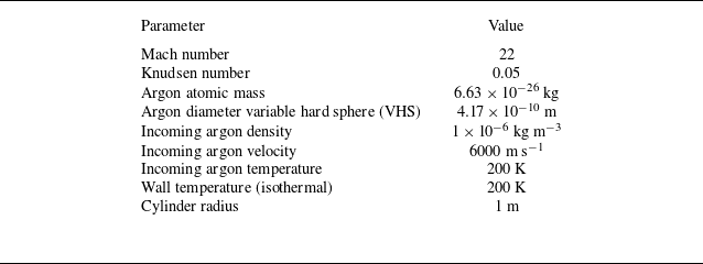
For the fluid field simulation, the cylinder radius is $ r = 1$ m. The computational mesh is generated by extrusion, with a first-layer height of approximately $ 0.02r$ and a total of 5000 cells, as shown in figure 4(a). For the electromagnetic field simulation, the same cylinder geometry is used, but with a different mesh, as illustrated in figure 4(b). The fluid solution is interpolated onto the electromagnetic mesh, which is then refined to 5 120 000 cells, corresponding to more than 100 points per wavelength, to ensure numerical accuracy. Table 2 lists the flow parameters. The Knudsen number is normalised by the diameter of the cylinder L = 2 m.

Table 2.

Simulation parameters for the rarefied argon flow around a cylinder.

Figure 4.

Computational domain and mesh for (a) the flow field and (b) the electromagnetic field.

Figure 5 compares the temperature and electron number density contours from GKS (upper half) and UGKWP (lower half). In this transitional regime, significant non-equilibrium effects are observed. As shown in figure 5(a), UGKWP predicts a broader temperature distribution than GKS, reflecting its enhanced non-equilibrium transport capability relative to the purely diffusion-based GKS. Figure 5(b) shows the electron number density contours on a logarithmic scale. Two differences are notable: first, UGKWP predicts a broader extension of the ionised region into the upstream stagnation zone, consistent with the extended preheating layer captured by the temperature field; second, in the wake region, UGKWP yields higher temperature and then electron number densities than GKS, which is consistent with literature results (Lofthouse et al. Reference Lofthouse, Scalabrin and Boyd2008; Long et al. Reference Long, Cao, Zhang and Xu2026). Figure 6 presents the local Knudsen number contours and its profile along the stagnation line. Three distinct peaks of $\textit{Kn}_{\textit{Gll}}$ are observed: one across the shock layer, where the flow field varies rapidly, one within the boundary layer and one in the wake region. The peak value exceeds $0.4$ , indicating that the flow locally exceeds the continuum regime. This suggests that a kinetic description is required in these regions.

Figure 7 compares the heavy-particle temperature and number density along the stagnation line predicted by GKS and UGKWP. The UGKWP results exhibit a pronounced increase in heavy-particle number density immediately adjacent to the wall, which enhances near-wall ionisation and consequently leads to a higher electron number density than that predicted by GKS, as shown in figure 8. This density enhancement may arise from non-local kinetic transport, whereby a fraction of heavy particles traverse the shock layer and penetrate into the near-wall region while retaining their wall-directed momentum, before collisions fully randomise their motion – an effect that may be underestimated by the near-equilibrium GKS description.

Elsewhere within the boundary layer, however, UGKWP predicts consistently lower temperatures than GKS, and GKS yields higher electron densities. This behaviour also arises from the distinct capability of each scheme to capture non-equilibrium transport. In GKS, the cold-wall effect remains confined to a very thin layer adjacent to the wall. The UGKWP, by contrast, captures non-local non-equilibrium transport, allowing the cold-wall influence to extend farther into the flow field. Meanwhile, the particle density reaches its maximum within the boundary layer due to strong compression, making this region the most favourable for ionisation. Given that the higher temperature predicted by GKS, combined with the high local density, promotes significantly more ionisation, GKS predicts higher electron number densities.

Figure 5.

(a) Heavy-particle temperature and (b) electron number density contours at Kn = 0.05. The upper and lower halves correspond to the GKS and UGKWP solutions, respectively.

Figure 6.

Local Knudsen number (a) contour and (b) profile along the stagnation line.

Figure 7.

(a) Heavy-particle temperature and (b) number density along the stagnation line at Kn = 0.05.

Figure 8.

Electron number density along the stagnation line at Kn = 0.05.

Figure 9 presents the electron number density along circular arcs at radii (a) $r=1.01$ and (b) $r=1.03$ m around the cylinder. In both cases, the UGKWP predictions exceed the GKS results, with the discrepancy increasing as the surface approaches the wall. This near-wall enhancement is associated with the higher heavy-particle number density predicted by UGKWP, which promotes ionisation and leads to stronger local shielding than that predicted by GKS.

Figure 9.

Electron number density along circular arcs at radii (a) $r = 1.01$ m and (b) $r = 1.03$ m.

6. Electromagnetic-wave scattering by the plasma layer

Based on the computed flow fields, we next simulate electromagnetic-wave propagation to compare the scattering characteristics. The electromagnetic calculations are intended to provide a qualitative illustration of how rarefaction-induced changes in the plasma distribution affect wave propagation, rather than a quantitative evaluation of the global reflection and transmission coefficients.

The simulations are configured as follows. A transverse magnetic plane wave enters the domain at frequency $f$ with components $E_z = \sin (2\pi f t)$ and $B_y = E_z / c$ , where $c$ denotes the speed of light. Two incident frequencies, 1.2 and 0.9 GHz, and two propagation directions –in the positive $x$ -direction (from $(-1,0)$ to $(1,0)$ ) and at a $45\,^{\circ }$ angle relative to the negative $x$ -axis (from $(1,1)$ to $(-1,-1)$ ) – are considered. The mesh setting is shown in the previous § 5 in figure 4(b). Absorbing boundary conditions are applied at the remaining boundaries to minimise spurious reflections. The cylinder surface is modelled as a perfect electrical conductor. All electromagnetic simulations are run up to a time of 2 $\times \text{10}^{-8}\text{s}$ , corresponding to 24 and 18 complete wave periods for 1.2 and 0.9 GHz, respectively. Therefore, the instantaneous fields are compared at the same phase of the incident wave.

We first examine a high-frequency case at $f = 1.2\ \text{GHz}$ , in which the wave enters from the left boundary and propagates along the (−1,0) to (1,0) direction. The corresponding critical electron number density is approximately $1.8 \times 10^{16}\ \text{m}^{-3}$ . At this frequency, the wave propagates freely through most of the shock layer, where the local electron number density remains below the critical value. Significant reflection occurs only in the immediate vicinity of the cylinder surface, where the electron number density exceeds the cutoff threshold.

Figure 10 presents the corresponding contours of permittivity and conductivity, defined as

(6.1) \begin{align} \varepsilon = \varepsilon _0 \left (1 - \frac {\omega _p^2}{\omega ^2 + \nu _{eh}^2}\right ),\qquad \sigma _c = \frac {\varepsilon _0 \omega _p^2 \nu _{eh}}{\omega ^2 + \nu _{eh}^2}, \end{align}

where $\omega = 2\pi f$ is the angular frequency. The upper half of each contour uses the GKS flow field, and the lower half uses the UGKWP results. As shown in figure 10(a), negative permittivity is confined to the region immediately adjacent to the cylinder surface; elsewhere, the permittivity remains positive, allowing wave transmission. The upper half exhibits more negative permittivity than the lower half, reflecting the higher peak electron number density in the GKS solution. Similarly, GKS-based plasma field produces larger conductivity around the main electron-density peak in the stagnation shock layer, whereas UGKWP-based plasma field yields locally enhanced conductivity in the region immediately adjacent to the wall.

Figure 11 compares the magnitudes of the electric and magnetic fields. The upper half of each contour corresponds to the GKS-based plasma profile, and the lower half to the UGKWP-based profile. The wave propagates through most of the shock layer and decays only in the immediate vicinity of the cylinder surface, where the electron number density exceeds the critical value. The amplitude enhancement observed within the plasma layer may be attributed to resonance effects associated with evanescent wave behaviour (White & Chen Reference White and Chen1974).

Figure 12(a) shows the $E_z$ profile along the stagnation line. At the selected phase, the GKS-based plasma profile exhibits a more pronounced reflected-wave pattern along the stagnation line, consistent with its higher peak electron number density. Figure 12(b) presents the field distribution along a circular arc at $r=1.01$ m. Near the cylinder surface, UGKWP predicts a lower instantaneous field amplitude than GKS. This behaviour is consistent with the higher near-wall electron density, as shown in figure 8, indicating stronger local shielding and reduced field penetration. Consequently, UGKWP predicts stronger near-wall shielding, whereas GKS exhibits a stronger reflection tendency in the stagnation shock layer.

Figure 10.

(a) Permittivity $\varepsilon$ and (b) conductivity $\sigma _c$ at $f = 1.2\ \text{GHz}$ . The upper and lower halves correspond to the GKS and UGKWP flow fields, respectively.

Figure 11.

The (a) $|\boldsymbol{E}|$ and (b) $|\boldsymbol{B}|$ contours at $f = 1.2\ \text{GHz}$ . The upper and lower halves correspond to the GKS and UGKWP flow fields, respectively.

Figure 12.

The $E_z$ profiles (a) along the stagnation line and (b) along a circular arc at $r = 1.01$ m, at $f = 1.2\ \text{GHz}$ .

We next examine a lower-frequency case at $f = 0.9\ \text{GHz}$ . The corresponding critical electron number density is approximately $1.0 \times 10^{16}\ \text{m}^{-3}$ . Figure 13 shows the permittivity and conductivity contours at this frequency. Compared with the 1.2 GHz case (figure 10 a), the negative-permittivity region expands significantly, consistent with the lower cutoff frequency. The conductivity contours (figure 13 b) exhibit a similar trend, showing larger values in the same near-wall region.

Figure 14 shows the electromagnetic field magnitude contours at $f = 0.9\ \text{GHz}$ . At this frequency, the blackout region expands significantly, as evident in figure 14(a). The stagnation-line profile, shown in figure 15(a), exhibits a similar trend to the 1.2 GHz case: GKS reflects more signal than UGKWP, consistent with its higher peak electron number density. Figure 15(b) presents the $E_z$ field along a circular arc at $r = 1.03$ m. Near the stagnation region (0 degrees), UGKWP predicts a weaker signal than GKS, but the trend reverses in the wake, where the UGKWP signal gradually exceeds that of GKS.

Figure 13.

(a) Permittivity $\varepsilon$ and (b) conductivity $\sigma _c$ at $f = 0.9\ \text{GHz}$ . The upper and lower halves correspond to the GKS and UGKWP flow fields, respectively.

Figure 14.

The (a) $|\boldsymbol{E}|$ and (b) $|\boldsymbol{B}|$ contours at $f = 0.9\ \text{GHz}$ . The upper and lower halves correspond to the GKS and UGKWP flow fields, respectively.

Figure 15.

The $E_z$ profiles (a) along the stagnation line and (b) along a circular arc at $r = 1.03$ m, at $f = 0.9\ \text{GHz}$ .

In both frequency cases, a consistent trend emerges: GKS predicts stronger reflection tendency in the stagnation region due to its higher peak electron number density, while UGKWP predicts more severe signal attenuation tendency near the cylinder surface. These contrasting behaviours arise from the inability of the continuum GKS model to capture the non-equilibrium transport processes that govern the boundary-layer structure and thus ionisation distribution.

We next consider a case where the incident wave propagates from the $(1,1)$ to the $(-1,-1)$ direction at 0.9 GHz, as shown in figure 16. In contrast to the previous case with wave propagation along the $(-1,0)$ to $(1,0)$ direction (figure 14), the signal now reaches the cylinder surface. This is because the electron number density in the wake region is lower than in the stagnation region, as seen in figure 5(b). Despite both methods predicting wave transmission, the GKS and UGKWP results differ much more significantly in this oblique-incidence case than in the previous one. The magnitude and phase of the electromagnetic fields show distinctly different distributions. This discrepancy arises from the larger deviations in electron number density predicted by the two methods in the wake region, where the flow becomes more rarefied (figure 6 a). In this region, the continuum assumption fails, leading to substantial differences between the two predictions. These results highlight the importance of using a multiscale method to accurately predict the flow field in the wake region.

Figure 16.

The (a) $|\boldsymbol{E}|$ and (b) $|\boldsymbol{B}|$ contours at $f = 0.9\ \text{GHz}$ . The incident wave direction comes from (1,1) to (−1,−1). The upper and lower halves correspond to the GKS and UGKWP flow fields, respectively.