1 Introduction
Flows driven between differentially rotating disks have a long history due to their relevance to many processes in nature and technology, as well as being of fundamental interest (Batchelor Reference Batchelor1951; Stewartson Reference Stewartson1953; Rott & Lewellen Reference Rott and Lewellen1966; Zandbergen & Dijkstra Reference Zandbergen and Dijkstra1987; Lopez Reference Lopez1998; Launder, Poncet & Serre Reference Launder, Poncet and Serre2010). The fundamental issue concerning the nature of the bulk flow between differentially rotating disks depends critically on the lateral conditions at large radii, and for enclosed systems, the sidewall boundary condition plays a major role in determining the bulk flow, due to the induced meridional flow. For the most part, these types of flows have been studied in cylindrical containers, and when the differential rotation is sufficiently strong, the axisymmetry of the flow is broken leading to rotating waves, modulated rotating waves and other spatio-temporally complicated states (Blackburn & Lopez Reference Blackburn and Lopez2000, Reference Blackburn and Lopez2002; Gauthier et al. Reference Gauthier, Gondret, Moisy and Rabaud2002; Lopez et al. Reference Lopez, Hart, Marques, Kittelman and Shen2002; Marques, Gelfgat & Lopez Reference Marques, Gelfgat and Lopez2003; Lopez & Marques Reference Lopez and Marques2004; Moisy et al. Reference Moisy, Doaré, Pasutto, Daube and Rabaud2004; Lopez Reference Lopez2006).
The case when the two endwalls (disks) are exactly in counter rotation and the sidewall is stationary, the so-called von Kármán swirling flow, is special as the system is more than just axisymmetric (invariance to rotations about the axis,
 $SO(2)$
symmetry), it is also invariant to a
 $Z_{2}$
symmetry (involution). This involution is a combination of a reflection through any meridional plane composed with a reflection about the mid-plane (Nore et al.
Reference Nore, Tuckerman, Daube and Xin2003, Reference Nore, Tartar, Daube and Tuckerman2004, Reference Nore, Witkowski, Foucault, Pécheux, Daube and Le Quéré2006), and is equivalent to a rotation of
 $\unicode[STIX]{x03C0}$
about an axis through the centre of the cylinder that is orthogonal to the cylinder axis. This involution does not commute with the rotation, and together these symmetries form an
 $O(2)$
symmetry group. In general, differentially rotating cylinder flows only have
 $SO(2)$
symmetry, and it is well established that flows with
 $O(2)$
symmetry can have fundamentally different behaviour to flows with
 $SO(2)$
symmetry (Crawford & Knobloch Reference Crawford and Knobloch1991; Knobloch Reference Knobloch1996). In particular, when axisymmetry is broken in an
 $SO(2)$
system, rotating waves result, whereas in
 $O(2)$
systems, steady three-dimensional states can result.
The flow in a cylinder with exactly counter-rotating endwalls and a stationary sidewall, the von Kármán swirling flow, has attracted much attention as a possible laboratory-scale dynamo. The motivation comes from the torsional forcing of the counter-rotating endwalls providing a global-scale dynamo action. However, the stationary sidewall imparts significant viscous drag, substantially reducing the effectiveness of the counter-rotating endwalls driving a torsional flow. Experimentally, the flat endwalls are replaced by impellers to counteract the sidewall effects (Bourgoin et al.
Reference Bourgoin, Marié, Pétrélis, Gasquet, Guigon, Luciani, Moulin, Namer, Burguete and Chiffaudel2002; Ravelet et al.
Reference Ravelet, Marie, Chiffaudel and Daviaud2004; Monchaux et al.
Reference Monchaux, Berhanu, Bourgoin, Moulin, Odier, Pinton, Volk, Fauve, Mordant and Pétrélis2007; de la Torre & Burguete Reference de la Torre and Burguete2007; Ravelet et al.
Reference Ravelet, Monchaux, Aumaître, Chiffaudel, Daviaud, Dubrulle, Bourgoin, Odier, Plihon and Pinton2008; Crespo del Arco et al.
Reference Crespo del Arco, Sánchez-Álvarez, Serre, de la Torre and Burguete2009; Giesecke, Stefani & Burguete Reference Giesecke, Stefani and Burguete2012). The
 $O(2)$
symmetry of the problem leads to interesting dynamics when it is broken, resulting from mode interactions which have strong spatial resonances. Nore et al. (Reference Nore, Tuckerman, Daube and Xin2003) studied the competition between states with azimuthal wavenumbers
 $m=1$
and 2. Such 1 : 2 resonances have drawn considerable attention from a dynamical systems perspective as there are associated robust heteroclinic cycles in reduced-order models (normal form equations) of such systems (Dangelmayr Reference Dangelmayr1986; Jones & Proctor Reference Jones and Proctor1987; Armbruster, Guckenheimer & Holmes Reference Armbruster, Guckenheimer and Holmes1988; Krupa Reference Krupa1990; Porter & Knobloch Reference Porter and Knobloch2001). In particular, Nore et al. (Reference Nore, Tuckerman, Daube and Xin2003) have found slow–fast dynamic states that they have associated with the heteroclinic cycles in the normal form model. Nore, Moisy & Quartier (Reference Nore, Moisy and Quartier2005) have observed such states in experiments, the so-called near-heteroclinic cycles, albeit influenced to some degree by noise and geometrical defects.
Here, we study a flow related to the von Kármán swirling flow, with the essential difference being that instead of having a stationary sidewall, the sidewall is split at the half-height, with each half rotating with the corresponding endwall. This flow has significantly less sidewall drag on the global torsional flow since the split sidewall halves also counter rotate at the same rate as their corresponding endwalls, and so may provide an enhanced dynamo action. This configuration has the same
 $O(2)$
symmetry as the von Kármán swirling flow, but the shear at mid-height is much stronger for the same aspect ratio and rotation rates of the endwalls. As in the von Kármán swirling flow, the primary instabilities are dominated by the dynamics associated with
 $O(2)$
symmetry breaking, mode interactions and competitions, but in the split sidewall flow these occur at significantly lower Reynolds numbers (non-dimensional endwall rotation rates). Over a considerable portion of the range of Reynolds numbers and aspect ratios considered, the dynamics is dominated by pulse wave states that are associated with the
 $O(2)$
symmetry breaking.
2 Governing equations and numerical methods
The flow of a fluid of kinematic viscosity
 $\unicode[STIX]{x1D708}$
contained in a rotating split cylinder is studied numerically. The cylinder of radius
 $a$
and length
 $h$
is split in two at mid-height and the two halves are counter-rotating with angular speeds
 $\pm \unicode[STIX]{x1D714}$
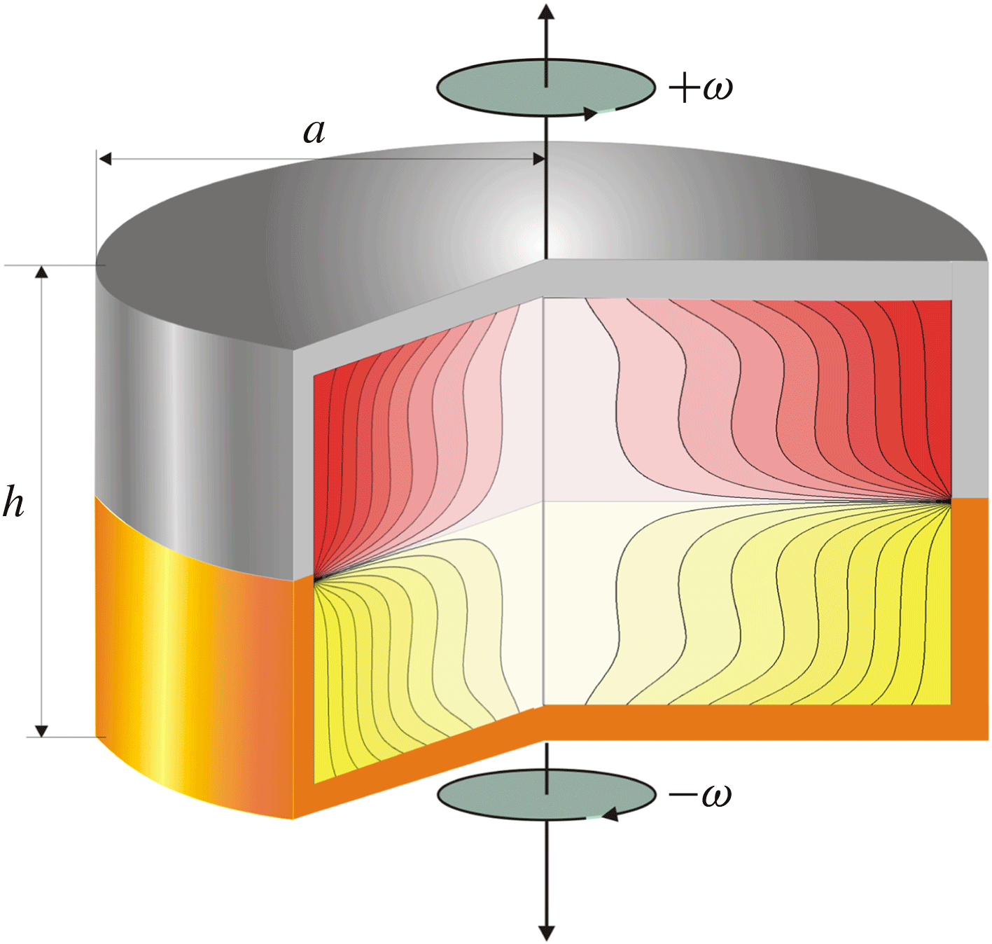
. A schematic of the problem is shown in figure 1. Using
 $a$
as the length scale and
 $a^{2}/\unicode[STIX]{x1D708}$
as the time scale, the non-dimensional Navier–Stokes equations are
 $$\begin{eqnarray}(\unicode[STIX]{x2202}_{t}+\boldsymbol{u}\boldsymbol{\cdot }\unicode[STIX]{x1D735})\boldsymbol{u}=-\unicode[STIX]{x1D735}p+\unicode[STIX]{x1D6FB}^{2}\boldsymbol{u},\quad \unicode[STIX]{x1D735}\boldsymbol{\cdot }\boldsymbol{u}=0.\end{eqnarray}$$
The no-slip boundary conditions are:
 $$\begin{eqnarray}\left.\begin{array}{@{}c@{}}(u,v,w)=(0,r\mathit{Re},0)~\text{at the top endwall},z=0.5\unicode[STIX]{x1D6E4},\\ (u,v,w)=(0,-r\mathit{Re},0)~\text{at the bottom endwall},z=-0.5\unicode[STIX]{x1D6E4},\\ (u,v,w)=(0,\mathit{Re},0)~\text{at the top half of the sidewall},r=1,z\in (0,0.5\unicode[STIX]{x1D6E4}),\\ (u,v,w)=(0,-\mathit{Re},0)~\text{at the bottom half of the sidewall},r=1,z\in (-0.5\unicode[STIX]{x1D6E4},0),\end{array}\right\}\end{eqnarray}$$
where the two governing parameters are
 $$\begin{eqnarray}\left.\begin{array}{@{}ll@{}}\text{aspect ratio:} & \unicode[STIX]{x1D6E4}=h/a,\\ \text{Reynolds number:} & \mathit{Re}=\unicode[STIX]{x1D714}a^{2}/\unicode[STIX]{x1D708}.\end{array}\right\}\end{eqnarray}$$
In polar coordinates
 $(r,\unicode[STIX]{x1D703},z)\in [0,1]\times [0,2\unicode[STIX]{x03C0}]\times [-0.5\unicode[STIX]{x1D6E4},0.5\unicode[STIX]{x1D6E4}]$
, the velocity is
 $\boldsymbol{u}=(u,v,w)$
and the vorticity is
 $\unicode[STIX]{x1D735}\times \boldsymbol{u}=(\unicode[STIX]{x1D712},\unicode[STIX]{x1D702},\unicode[STIX]{x1D701})=(w_{\unicode[STIX]{x1D703}}/r-v_{z},u_{z}-w_{r},v_{r}+v/r-u_{\unicode[STIX]{x1D703}}/r)$
.
Schematic of the flow system. The inset shows contours of
 $rv$
(vortex lines) for a basic state at
 $(\unicode[STIX]{x1D6E4},\mathit{Re})=(1,115)$
. There are ten quadratically spaced contour levels of
 $rv\in [-\mathit{Re},\mathit{Re}]$
, with positive being red and negative being yellow.

The Navier–Stokes equations are solved using a spectral code based on Mercader, Batiste & Alonso (Reference Mercader, Batiste and Alonso2010), using a second-order time-splitting method and space discretized via a Galerkin–Fourier expansion in
 $\unicode[STIX]{x1D703}$
and Chebyshev collocation in
 $r$
and
 $z$
:
 $$\begin{eqnarray}\boldsymbol{u}(r,\unicode[STIX]{x1D703},z,t)=\mathop{\sum }_{i=0}^{2n_{r}+1}\mathop{\sum }_{j=0}^{n_{z}}\mathop{\sum }_{k=-0.5n_{\unicode[STIX]{x1D703}}}^{k=0.5n_{\unicode[STIX]{x1D703}}-1}\hat{\boldsymbol{u}}_{ijk}(t)\unicode[STIX]{x1D6EF}_{i}(r)\unicode[STIX]{x1D6EF}_{j}(2z/\unicode[STIX]{x1D6E4})\text{e}^{\text{i}k\unicode[STIX]{x1D703}},\end{eqnarray}$$
where
 $\unicode[STIX]{x1D6EF}_{n}$
is the
 $n$
th Chebyshev polynomial. The modal kinetic energies corresponding to azimuthal wavenumbers
 $m$
are
 $$\begin{eqnarray}E_{m}=\frac{1}{2}\int _{-0.5\unicode[STIX]{x1D6E4}}^{0.5\unicode[STIX]{x1D6E4}}\int _{0}^{1}\boldsymbol{u}_{m}\boldsymbol{\cdot }\boldsymbol{u}_{m}^{\ast }r\,\text{d}r\,\text{d}z,\end{eqnarray}$$
where
 $\boldsymbol{u}_{m}$
is the
 $m$
th Fourier component of the velocity field and
 $\boldsymbol{u}_{m}^{\ast }$
is its complex conjugate.
To avoid Gibb’s phenomenon due to the discontinuity in the sidewall boundary condition for the azimuthal velocity, we regularized the boundary condition by smoothing the discontinuity over a small distance. Specifically, we replaced the boundary condition for the azimuthal velocity with
 $$\begin{eqnarray}v(r=1,\unicode[STIX]{x1D703},z)=\mathit{Re}\tanh (\unicode[STIX]{x1D716}z),\end{eqnarray}$$
where
 $\unicode[STIX]{x1D716}$
governs the distance over which the jump is smoothed;
 $\unicode[STIX]{x1D716}=50$
was used in this study, as was done in related rotating split-cylinder problems (Gutierrez-Castillo & Lopez Reference Gutierrez-Castillo and Lopez2015; Lopez & Gutierrez-Castillo Reference Lopez and Gutierrez-Castillo2016). A spatial resolution of
 $n_{r}=40$
,
 $n_{z}=160$
and
 $n_{\unicode[STIX]{x1D703}}=64$
, and a time resolution of
 $\unicode[STIX]{x1D6FF}_{t}\in [10^{-4},10^{-5}]$
was used for the parameter range studied,
 $\unicode[STIX]{x1D6E4}\in [0.5,2.0]$
and
 $\mathit{Re}\in [100,300]$
. In this parameter range, the resolution used results in spectral convergence in the coefficients in (2.4) of over sixteen orders of magnitude in
 $\unicode[STIX]{x1D703}$
, six orders of magnitude in
 $r$
and three orders of magnitude in
 $z$
. The slower convergence in
 $z$
is due to using the
 $L_{\infty }$
norm; the convergence is slowest in the neighbourhood of the sidewall split, but this slow convergence is very localized and constrained by the viscous boundary layer. The convergence in
 $z$
away from the split is comparable to that in
 $r$
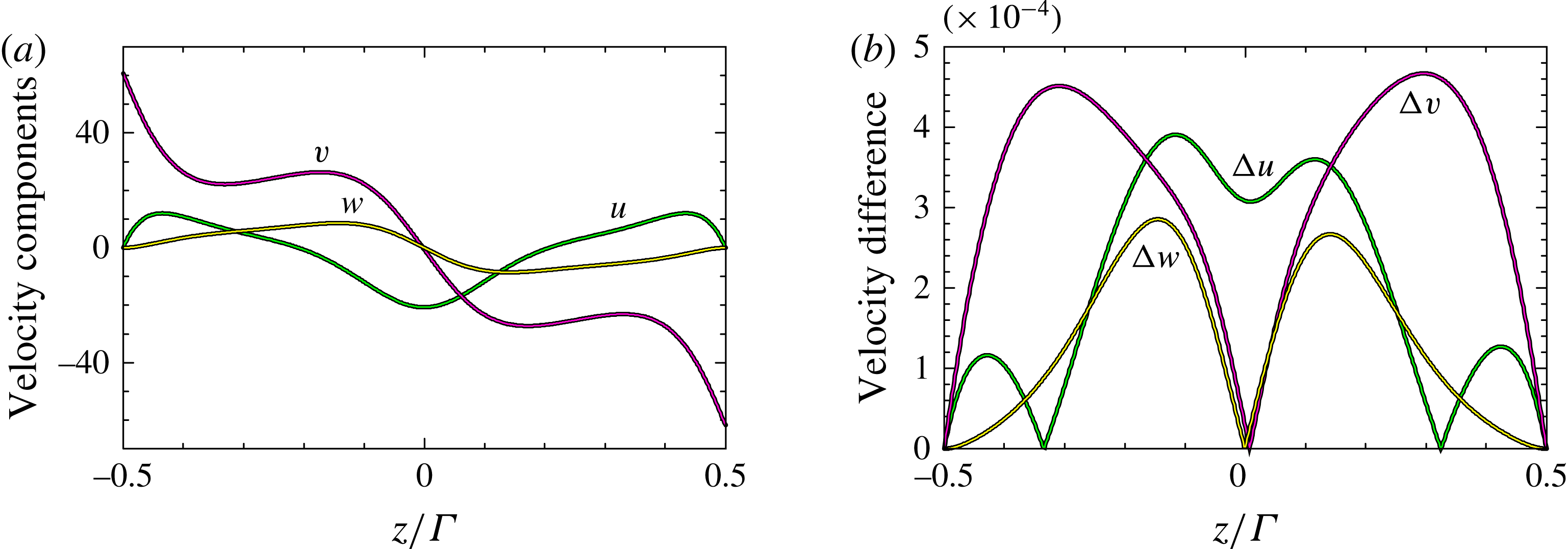
. Also, with this resolution, there are at least 15 collocation points across boundary layers, resulting in very well resolved solutions. Figure 2 illustrates how well the solutions are resolved by presenting the axial velocity profiles of the three velocity components at
 $r=0.5$
and
 $\unicode[STIX]{x1D703}=0$
of a typical state, S2 at
 $(\unicode[STIX]{x1D6E4},\mathit{Re})=(1.45,123)$
, computed with
 $n_{r}=40$
,
 $n_{\unicode[STIX]{x1D703}}=64$
and either
 $n_{z}=120$
(thick black curves) or
 $n_{z}=160$
(thin coloured curves). On the scale of the plot, the two solutions are indistinguishable. Also shown in the figure are the absolute differences between the three velocity components computed with the two resolutions, showing that the difference resulting from a 33 % increase in the axial resolution, from
 $n_{z}=120$
to
 $n_{z}=160$
, only affects the solution in the fifth significant digit in the interior.
(a) Axial (
 $z$
) profiles of the three velocity components at
 $r=0.5$
and
 $\unicode[STIX]{x1D703}=0$
of S2 at
 $(\unicode[STIX]{x1D6E4},\mathit{Re})=(1.45,123)$
computed with
 $n_{r}=40$
,
 $n_{\unicode[STIX]{x1D703}}=64$
and either
 $n_{z}=120$
(thick black curves) or
 $n_{z}=160$
(thin coloured curves), and (b) the absolute differences between the three velocity component computed with the two resolutions.

The system (2.1) and (2.2) is invariant to two spatial symmetries and a time translation
 ${\mathcal{T}}_{\unicode[STIX]{x1D6FD}}$
. One spatial symmetry is
 ${\mathcal{R}}_{\unicode[STIX]{x1D6FC}}$
, the invariance to arbitrary rotations about the cylinder axis. It is isomorphic to the
 $SO(2)$
symmetry group. The other spatial symmetry is
 ${\mathcal{H}}_{\unicode[STIX]{x1D6FE}}$
, the combined action of a reflection in any meridional plane
 $\unicode[STIX]{x1D703}=\unicode[STIX]{x1D6FE}$
and a reflection in the mid-plane
 $z=0$
. This combined reflection is equivalent to a rotation of
 $\unicode[STIX]{x03C0}$
about a direction through the centre of the cylinder that is orthogonal to the cylinder axis and in the
 $\unicode[STIX]{x1D703}=\unicode[STIX]{x1D6FE}$
plane. The
 ${\mathcal{H}}_{\unicode[STIX]{x1D6FE}}$
involution is isomorphic to the
 $Z_{2}$
symmetry group; applying it twice is equivalent to the identity operation. The actions of
 ${\mathcal{R}}_{\unicode[STIX]{x1D6FC}}$
,
 ${\mathcal{H}}_{\unicode[STIX]{x1D6FE}}$
, and
 ${\mathcal{T}}_{\unicode[STIX]{x1D6FD}}$
on the velocity are
 $$\begin{eqnarray}\left.\begin{array}{@{}c@{}}{\mathcal{R}}_{\unicode[STIX]{x1D6FC}}(u,v,w)(r,\unicode[STIX]{x1D703},z,t)=(u,v,w)(r,\unicode[STIX]{x1D703}+\unicode[STIX]{x1D6FC},z,t),\quad \unicode[STIX]{x1D6FC}~\text{arbitrary},\\ {\mathcal{H}}_{\unicode[STIX]{x1D6FE}}(u,v,w)(r,\unicode[STIX]{x1D703},z,t)=(u,-v,-w)(r,2\unicode[STIX]{x1D6FE}-\unicode[STIX]{x1D703},-z,t),\quad \unicode[STIX]{x1D6FE}~\text{arbitrary},\\ {\mathcal{T}}_{\unicode[STIX]{x1D6FD}}(u,v,w)(r,\unicode[STIX]{x1D703},z,t)=(u,v,w)(r,\unicode[STIX]{x1D703},z,t+\unicode[STIX]{x1D6FD}),\quad \unicode[STIX]{x1D6FD}~\text{arbitrary}.\end{array}\right\}\end{eqnarray}$$
The two spatial symmetries,
 ${\mathcal{R}}_{\unicode[STIX]{x1D6FC}}$
and
 ${\mathcal{H}}_{\unicode[STIX]{x1D6FE}}$
, do not commute, and together they are isomorphic to the
 $O(2)$
symmetry group.
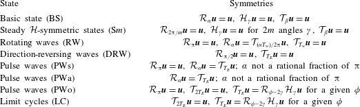
Summary of the different states and their symmetries. Note that
 $\unicode[STIX]{x1D6FC}$
,
 $\unicode[STIX]{x1D6FE}$
and
 $\unicode[STIX]{x1D6FD}$
are arbitrary unless otherwise indicated.

Much of the nonlinear dynamics involves the breaking of some aspects of the symmetries of the problem. Table 1 lists the various states encountered in this study together with their symmetries. Each is described in detail in the following section. It is useful to be able to compute the unstable flows following the symmetry-breaking bifurcations. This can be readily done by restricting the computations to invariant symmetric subspaces. The most useful subspaces for this problem are the subspaces
 $\unicode[STIX]{x1D709}_{m}$
, in which the flow is restricted to only having azimuthal wavenumbers
 $m=0$
and multiples of
 $m$
. Numerically, this is done by setting to zero the coefficients
 $\hat{\boldsymbol{u}}_{ijk}$
in (2.4) which do not correspond to these wavenumbers. There are two special such subspaces,
 $\unicode[STIX]{x1D709}_{0}$
which is the axisymmetric subspace and
 $\unicode[STIX]{x1D709}_{1}$
which is the full space.
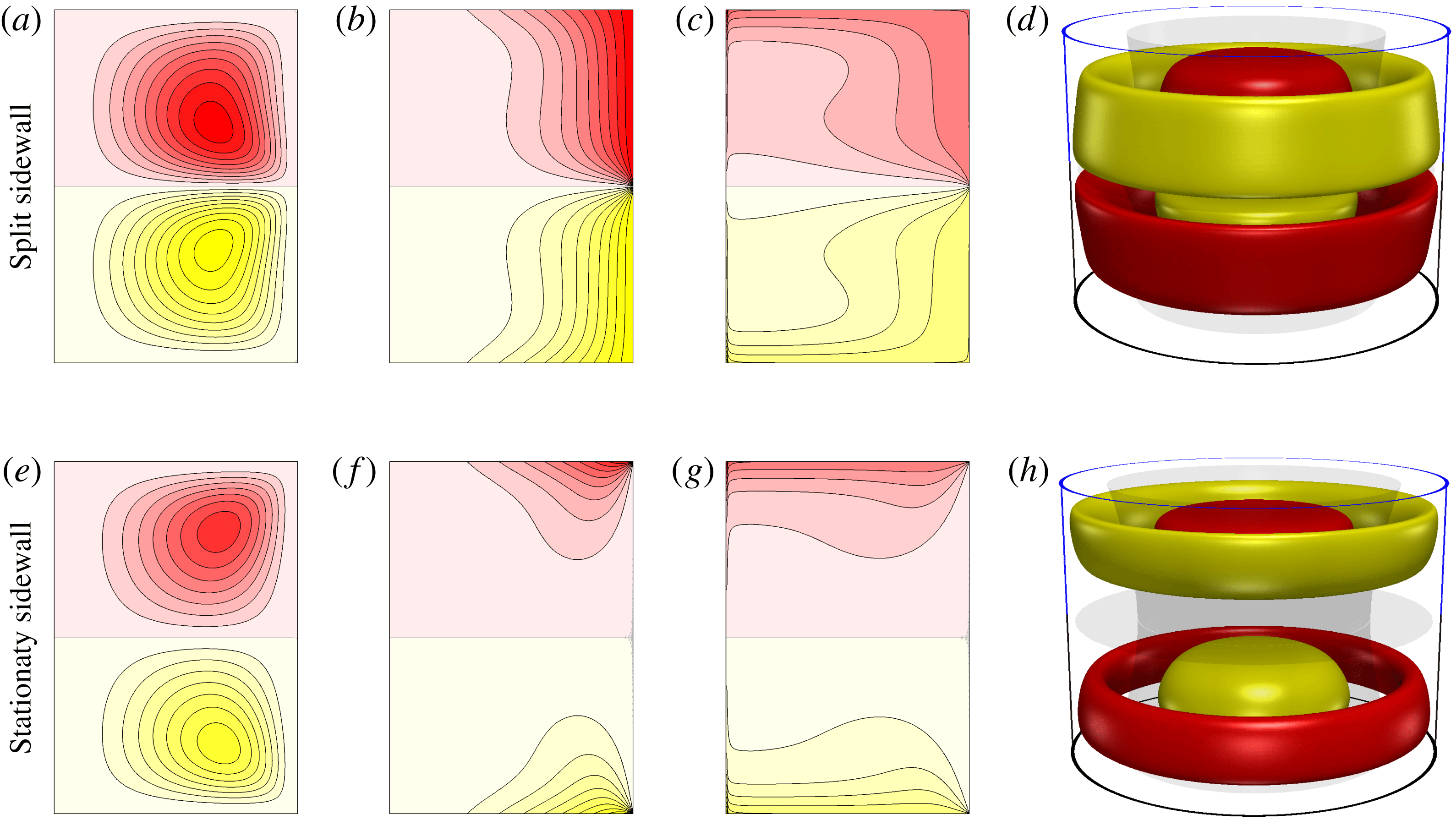
Contours in a meridional plane (
 $\unicode[STIX]{x1D703}=0$
,
 $r\times z\in [0,1]\times [-0.5\unicode[STIX]{x1D6E4},0.5\unicode[STIX]{x1D6E4}]$
) of (a)
 $\unicode[STIX]{x1D713}$
(streamlines), (b)
 $rv$
(vortex lines), (c)
 $v/r$
(angular velocity) and (d) isosurfaces of
 $w$
of BS at
 $(\unicode[STIX]{x1D6E4},\mathit{Re})=(1.45,115)$
for the split sidewall case (a–d) and the stationary sidewall case (e–h). The contour levels are linearly spaced (positive are red and negative are yellow) in the intervals
 $\unicode[STIX]{x1D713}\in [-1.25,1.25]$
,
 $rv\in [-\mathit{Re},\mathit{Re}]$
and
 $v/r\in [-2\mathit{Re},2\mathit{Re}]$
; the isosurfaces are at
 $w=\pm 0.05\mathit{Re}$
and at
 $w=0$
(translucent).

3 Results
In the following subsections, we begin describing the features of the basic state, and consider its primary instabilities to group orbits of steady states. Then, we study in detail the 2 : 3 mode interaction, primarily in the neighbourhood of the codimension-two (codim-2) point at
 $(\unicode[STIX]{x1D6E4},\mathit{Re})=(1.30,129.5)$
, and how some of the secondary bifurcation curves from that codim-2 point connect to the other 2 : 3 codim-2 point at
 $(\unicode[STIX]{x1D6E4},\mathit{Re})=(1.77,118.6)$
. We then consider in detail the dynamics as
 $\mathit{Re}$
is increased while keeping
 $\unicode[STIX]{x1D6E4}=1.45$
fixed. By computing not only in the full three-dimensional space
 $\unicode[STIX]{x1D709}_{1}$
, but also by restricting the simulations to various symmetry subspaces
 $\unicode[STIX]{x1D709}_{m}$
, we are able to provide a fairly complete picture of the complex dynamics involved. Finally, we provide a general overview of the various mode interactions and subsequent nonlinear dynamics over the broader parameter regime with
 $\unicode[STIX]{x1D6E4}\in [0.5,2.0]$
and
 $\mathit{Re}\in [100,300]$
.
Loci in
 $(\unicode[STIX]{x1D6E4},\mathit{Re})$
parameter space of circle-pitchfork bifurcations where BS loses stability to
 ${\mathcal{H}}$
-symmetric steady states
 $\text{S}m$
, with azimuthal wavenumber
 $m$
as indicated, upon crossing from low values of
 $\mathit{Re}$
and
 $\unicode[STIX]{x1D6E4}$
.

3.1 Basic state
The basic state, BS, is invariant to all symmetries of the system; it is steady and
 $O(2)$
symmetric. The streamlines (contours of
 $\unicode[STIX]{x1D713}$
, where
 $u=-1/r\,\unicode[STIX]{x2202}\unicode[STIX]{x1D713}/\unicode[STIX]{x2202}z$
and
 $w=1/r\,\unicode[STIX]{x2202}\unicode[STIX]{x1D713}/\unicode[STIX]{x2202}r$
), vortex lines (contours of
 $rv$
), contours of angular velocity
 $v/r$
and isosurfaces of the axial velocity
 $w$
of a typical BS at
 $(\unicode[STIX]{x1D6E4},\mathit{Re})=(1.45,115)$
are shown in the top row of figure 3. Note that for an axisymmetric velocity
 $(u,v,w)=(-1/r\,\unicode[STIX]{x2202}\unicode[STIX]{x1D713}/\unicode[STIX]{x2202}z,v,1/r\,\unicode[STIX]{x2202}\unicode[STIX]{x1D713}/\unicode[STIX]{x2202}r)$
and the corresponding vorticity is (
 $-1/r\,\unicode[STIX]{x2202}(rv)/\unicode[STIX]{x2202}z,\unicode[STIX]{x1D702}$
,
 $1/r\,\unicode[STIX]{x2202}(rv)/\unicode[STIX]{x2202}r$
), so that vortex lines in a meridional plane are tangent to the isocontours of
 $rv$
. The dominant feature of BS is the shear layer formed at the cylinder mid-height resulting in two meridional recirculation cells indicated by the streamlines. The flow in each half-cylinder would be in solid-body rotation (constant angular velocity), with opposing senses, if not for the presence of the flow in the other half-cylinder. These two counter-rotating bodies of fluid meet at the mid-plane
 $z=0$
and the vortex lines cannot be aligned with the axis at the mid-plane. The vortex lines emerge from the rotating endwalls and bend to be parallel to the mid-plane as they approach the split in the cylinder sidewall for the symmetric BS flow state. This vortex line bending produces the mid-plane shear layer and drives the meridional circulation, characterized by the streamlines in each cylinder half where flow is driven radially in toward the axis from the split in the sidewall along
 $z=0$
. By approximately mid-radius, the meridional flows turn toward the respective endwalls at
 $z=\pm 0.5\unicode[STIX]{x1D6E4}$
. The meridional flows in the endwall boundary layers are toward the sidewall. In the sidewall layer, the meridional flow is returned to the vicinity of the split at
 $z=0$
, completing the meridional circulation. A consequence of the meridional flows in the two halves is that the interior flows rotate slower than the respective endwalls, as evidenced from the angular velocity plot.
For comparison purposes, the corresponding plots for BS in the von Kármán swirling flow at the same
 $(\unicode[STIX]{x1D6E4},\mathit{Re})$
are shown in the bottom row of figure 3. The vortex lines still emerge from the rotating endwalls, but due to the sidewall being stationary, they terminate at the corners where the sidewall and the endwalls meet. This results in the azimuthal shear at the mid-plane,
 $\unicode[STIX]{x2202}v/\unicode[STIX]{x2202}z|_{z=0}$
, being much weaker than in the split-cylinder case, and the angular velocity in the interior is also considerably weaker. The resultant meridional flow is strongest near the corners where the vortex lines terminate, in contrast to the split sidewall case where the meridional flow is strongest near the sidewall split, which is where its vortex lines terminate. All in all, the split sidewall case produces a more intense azimuthal shear layer at mid-height with a stronger meridional jet flow at mid-height.
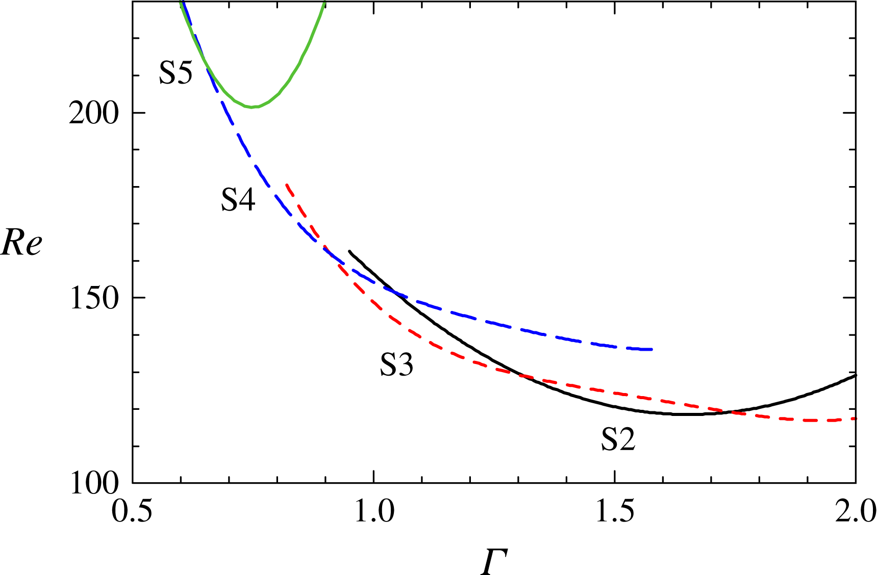
3.2 Circle-pitchfork bifurcations to steady
 ${\mathcal{H}}$
-symmetric states
$\text{S}m$


For small enough
 $\mathit{Re}$
, depending on
 $\unicode[STIX]{x1D6E4}$
, the steady
 $O(2)$
-symmetric BS flow is stable. Over the range of aspect ratios considered,
 $\unicode[STIX]{x1D6E4}\in [0.5,2.0]$
, the basic state BS loses stability as
 $\mathit{Re}$
is increased via circle-pitchfork bifurcations where the flow loses axisymmetry (the
 ${\mathcal{R}}_{\unicode[STIX]{x1D6FC}}$
invariance is broken), but remains steady (
 ${\mathcal{T}}_{\unicode[STIX]{x1D6FD}}$
invariant). Figure 4 shows the loci of the various circle-pitchfork bifurcations in (
 $\unicode[STIX]{x1D6E4},\mathit{Re}$
) parameter space. Although the continuous invariance
 ${\mathcal{R}}_{\unicode[STIX]{x1D6FC}}$
(with
 $\unicode[STIX]{x1D6FC}$
any angle) is broken, the flow retains a discrete invariance
 ${\mathcal{R}}_{2\unicode[STIX]{x03C0}/m}$
, where
 $m$
is the dominant azimuthal wavenumber of the flow. The value of
 $m$
depends on
 $\unicode[STIX]{x1D6E4}$
. We shall refer to these steady flows as
 $\text{S}m$
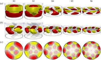
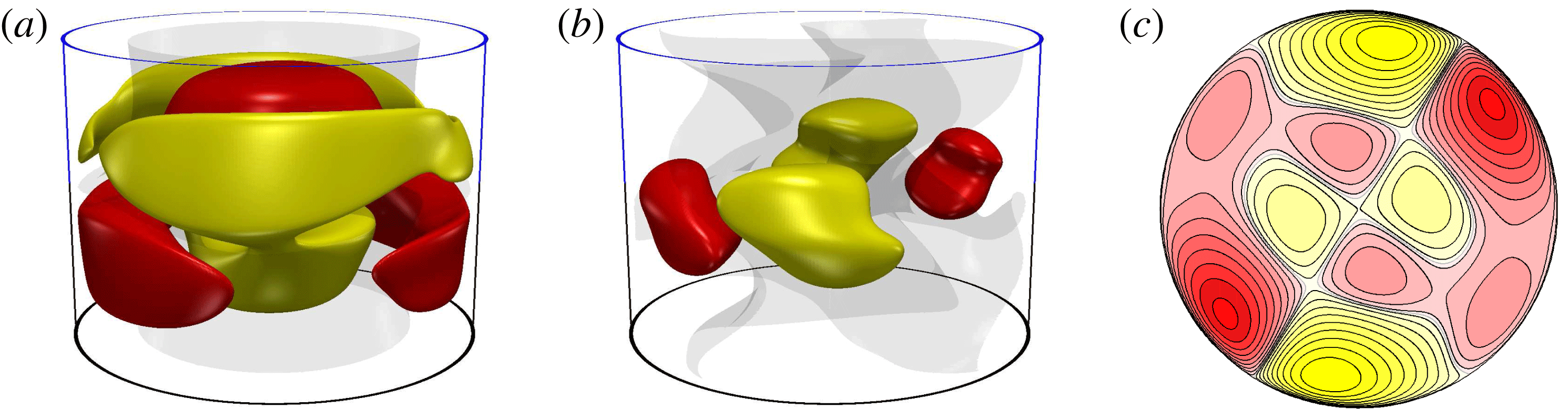
. Figure 5 shows typical
 $\text{S}m$
states, with
 $m\in [2,6]$
, where for each case, isosurfaces of the axial velocity
 $w$
, and of the non-axisymmetric component
 $w{-}w_{0}$
, where
 $w_{0}$
is the azimuthal average of
 $w$
, are shown, together with contours of
 $w$
at the mid-plane
 $z=0$
(note that for these steady states,
 $w_{0}=0$
at
 $z=0$
). The isosurface levels depicted in this and in subsequent figures are all at
 $\pm 0.4$
of the maximum of
 $w$
and
 $w{-}w_{0}$
, respectively. The contour levels of
 $w$
at the mid-plane are quadratically spaced in
 $\pm \max (w|_{z=0})$
, to enable comparisons between solutions at different points in
 $(\unicode[STIX]{x1D6E4},\mathit{Re})$
parameter space. The bifurcating states
 $\text{S}m$
are
 ${\mathcal{H}}_{\unicode[STIX]{x1D6FE}}$
invariant, but instead of
 $\unicode[STIX]{x1D6FE}$
being any angle, now there are only
 $2m$
angles differing by multiples of
 $\unicode[STIX]{x03C0}/m$
for which the states are
 ${\mathcal{H}}$
-symmetric. The angles are easily identified, they correspond to the orientations of the straight lines, along which
 $w=0$
, through the origin the cylinder mid-plane (see figure 5). For any
 $m$
, there is a group orbit of stationary
 ${\mathcal{H}}$
-symmetric states
 $\text{S}m$
with azimuthal wavenumber
 $m$
. All members of the group are obtained from any one of them by rotating it in azimuth, giving a whole circle of solutions. Which one is realized depends on initial conditions.
Isosurfaces of
 $w$
(a),
 $w{-}w_{0}$
(b) and contours of
 $w$
at
 $z=0$
(c), for S2 at
 $(\unicode[STIX]{x1D6E4},\mathit{Re})=(1.45,123)$
, S3 at
 $(\unicode[STIX]{x1D6E4},\mathit{Re})=(1.45,135)$
, S4 at
 $(\unicode[STIX]{x1D6E4},\mathit{Re})=(0.80,225)$
, S5 at
 $(\unicode[STIX]{x1D6E4},\mathit{Re})=(0.60,250)$
and S6 at
 $(\unicode[STIX]{x1D6E4},\mathit{Re})=(0.50,300)$
.

In summary the
 $\text{S}m$
have the invariances
 ${\mathcal{R}}_{2\unicode[STIX]{x03C0}/m}\boldsymbol{u}=\boldsymbol{u}$
,
 ${\mathcal{H}}_{\unicode[STIX]{x1D6FE}}\boldsymbol{u}=\boldsymbol{u}$
for
 $2m$
angles differing by multiples of
 $\unicode[STIX]{x03C0}/m$
, and
 ${\mathcal{T}}_{\unicode[STIX]{x1D6FD}}\boldsymbol{u}=\boldsymbol{u}$
for arbitrary
 $\unicode[STIX]{x1D6FD}$
.
For the von Kármán swirling flow, it has been suggested that the shear layer at mid-height in the basic state loses stability via a Kelvin–Helmholtz type of instability leading to steady states with azimuthal wavenumbers
 $m\approx 2/\unicode[STIX]{x1D6E4}$
(Nore et al.
Reference Nore, Tuckerman, Daube and Xin2003, Reference Nore, Tartar, Daube and Tuckerman2004). In our flow, we do not find strong evidence for this. Figure 4 shows that S2 bifurcates for
 $\unicode[STIX]{x1D6E4}\sim 1.5$
, and S3 bifurcates for both
 $\unicode[STIX]{x1D6E4}\sim 1$
and
 $\unicode[STIX]{x1D6E4}\sim 2$
, and both co-exist over a large range of
 $\unicode[STIX]{x1D6E4}$
. Another mechanism that is acting to make BS unstable is the counter rotation. Vortex lines in a rotating system have a tendency to align with the rotation axis. When the flow is axisymmetric, the exact counter rotation of the two halves of the cylinder results in the vortex lines being forced to be tangential to the mid-plane. By breaking axisymmetry, some of the vortex lines from one half can penetrate partially into the other half, resulting in the interface between the two counter-rotating bodies of fluid being undulated. The axial velocity
 $w$
at
 $z=0$
is a proxy for the interface undulation; this is shown in the third row of figure 5 for the different
 $\text{S}m$
found. Furthermore, for the Kelvin–Helmholtz instability of shear flow in a constant density fluid, the base flow velocity vector is planar two-dimensional and the vorticity vector is orthogonal to the velocity (i.e. the helicity, dot product of the velocity and vorticity vectors, is zero). In the problem under study, where the shear layer is due to counter-rotating bodies of fluid, the flow has non-zero helicity even in the absence of any instability, and the helicity is more intense when axisymmetry is broken. Large values of helicity indicate that the velocity and vorticity vectors are more aligned, and this leads to intensification of the vorticity via vortex stretching. Viscous dissipation can limit this process. In a related flow, consisting of a rotating cylinder with a counter-rotating top endwall (Lopez et al.
Reference Lopez, Hart, Marques, Kittelman and Shen2002), a shear layer emanating from the corner where the sidewall and the counter-rotating top meet separates the counter-rotating bodies of fluid. That flow loses axisymmetry at
 $\mathit{Re}$
approximately an order of magnitude larger than in the present split-cylinder arrangement. The instability is also associated with the vortex lines trying to align themselves with the rotation axis and in doing so they try to penetrate through the shear layer. With the larger
 $\mathit{Re}$
, this penetration is not as viscously damped, and the result is a number of funnels of counter-rotating fluid, intensified by vortex stretching, penetrating all the way to the opposite endwall boundary layer. This type of behaviour is also present in the split-cylinder problem, but the penetration is symmetric into both halves, and not as intense due to the viscous dissipation in the lower
 $\mathit{Re}$
flow.
The bifurcation curves in figure 4 indicate that there are several codim-2 points where two different circle-pitchfork bifurcation curves intersect. As is typical in many problems with
 $O(2)$
symmetry, these codim-2 points correspond to curves with wavenumbers
 $m$
and
 $m+1$
. These points organize the mode interaction dynamics. Dangelmayr (Reference Dangelmayr1986) has shown that these mode interactions lead to rather distinct behaviour depending on if
 $m=1$
or
 $m>1$
. The case
 $m=1$
gives rise to the 1 : 2 resonant interaction, which has attracted much theoretical interest and was found and studied in the von Kármán swirling flow by Nore et al. (Reference Nore, Tuckerman, Daube and Xin2003). In our flow for the range of
 $\unicode[STIX]{x1D6E4}$
considered, there is no circle-pitchfork bifurcation with
 $m=1$
. However, for
 $\unicode[STIX]{x1D6E4}\in (1.3,1.75)$
, a circle-pitchfork bifurcation with
 $m=2$
is flanked by two others with
 $m=3$
, and Dangelmayr (Reference Dangelmayr1986) showed that the 2 : 3 mode interaction also has distinct behaviour compared to mode interactions with higher wavenumbers.
3.3 The 2 : 3 mode interaction
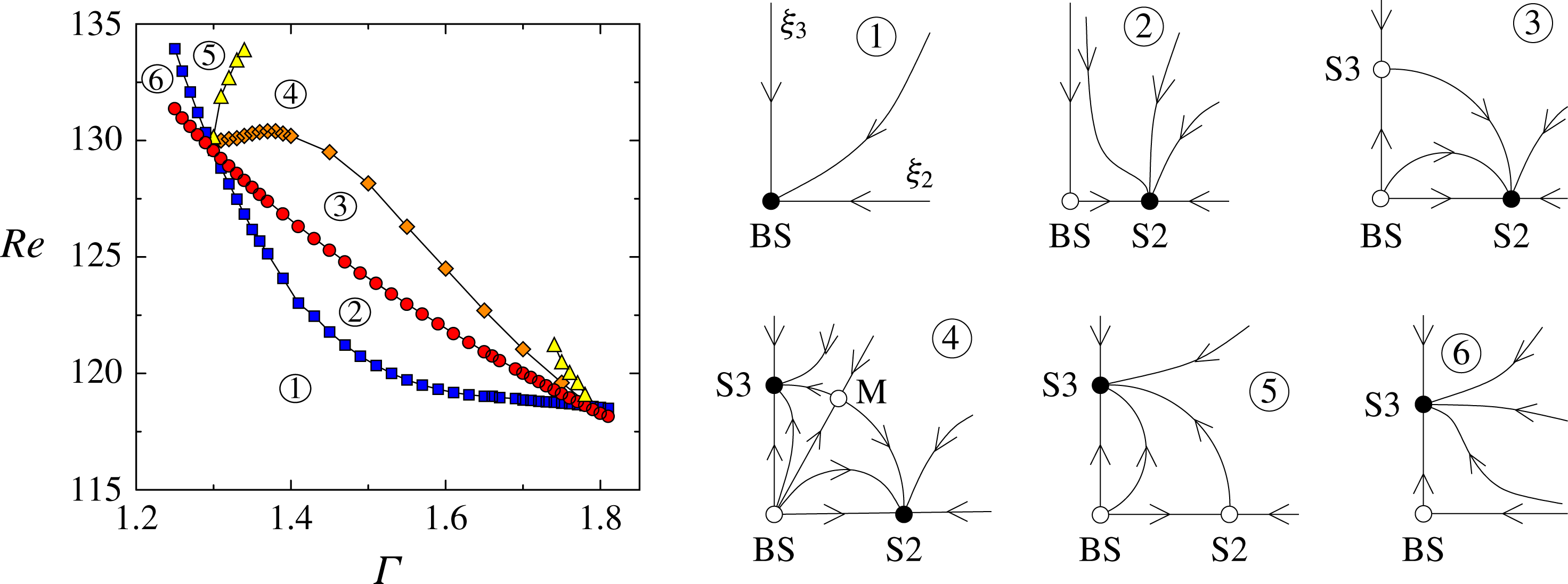
Figure 6 shows the circle-pitchfork bifurcation curves along which S2 and S3 bifurcate from BS together with schematics of phase portraits in distinct regions in the neighbourhood of the codim-2 point where S2 and S3 bifurcate simultaneously. Generically, these circle-pitchfork bifurcation curves either do not intersect or they intersect at two points (Dangelmayr Reference Dangelmayr1986; Higuera, Riecke & Silber Reference Higuera, Riecke and Silber2004). In figure 6, there are two such intersection points,
 $(\unicode[STIX]{x1D6E4},\mathit{Re})=(1.3,129.5)$
and
 $(1.78,118.7)$
. We now consider a circular parameter sweep around one of these codim-2 points. In region 1, BS is the unique solution and it is stable. On increasing
 $\mathit{Re}$
, BS loses stability to either S2 or S3, depending on
 $\unicode[STIX]{x1D6E4}$
. S2 and S3 belong to the subspaces
 $\unicode[STIX]{x1D709}_{2}$
and
 $\unicode[STIX]{x1D709}_{3}$
, respectively. Crossing from region 1 to region 2, the circle-pitchfork bifurcation renders BS unstable, and a stable group of S2 emerges. There are no other equilibria, stable or unstable, in region 2. Crossing into region 3 from region 2, BS undergoes another circle-pitchfork bifurcation and a group of S3 emerges and are unstable. Crossing from region 3 to region 4, S3 undergoes a steady-state bifurcation where it becomes stable. The normal form theory (see Dangelmayr Reference Dangelmayr1986; Higuera et al.
Reference Higuera, Riecke and Silber2004, for more details) says that two types of unstable mixed modes are spawned at the bifurcation (which we simply call M in the figure). These mixed modes have non-zero
 $m=2$
and
 $m=3$
azimuthal Fourier components. Since the mixed modes M are unstable and they do not reside in either the
 $\unicode[STIX]{x1D709}_{2}$
or
 $\unicode[STIX]{x1D709}_{3}$
subspace and they are not directly detectable.
Bifurcation curves near the 2 : 3 mode interaction, together with schematic phase portraits in the regions near the codim-2 point at
 $(\unicode[STIX]{x1D6E4},\mathit{Re})=(1.3,129.5)$
;
 $\unicode[STIX]{x1D709}_{2}$
and
 $\unicode[STIX]{x1D709}_{3}$
are the
 $m=2$
and
 $m=3$
subspaces.

Crossing from region 4 into region 5, another steady-state bifurcation takes place rendering S2 unstable (by absorbing the unstable mixed mode M). Crossing from region 5 to region 6, S2 is absorbed into BS at the circle-pitchfork bifurcation. In region 6, the only equilibria are the stable S3 and unstable BS. Crossing from region 6 back to region 1 completes the parameter sweep around the codim-2 point, and S3 is absorbed into BS at the circle-pitchfork bifurcation where BS regains stability. The two circle-pitchfork bifurcations where S2 and S3 bifurcate from BS were found by direct simulations in the
 $\unicode[STIX]{x1D709}_{2}$
and
 $\unicode[STIX]{x1D709}_{3}$
subspaces, respectively. The steady-state bifurcations where S2 and S3 change stability were found by simulations in the full space
 $\unicode[STIX]{x1D709}_{1}$
.
3.4 Parameter sweep in
$\mathit{Re}$
with
$\unicode[STIX]{x1D6E4}=1.45$


In order to investigate the nonlinear dynamics beyond the circle-pitchfork bifurcations, we focus on varying
 $\mathit{Re}$
while keeping
 $\unicode[STIX]{x1D6E4}=1.45$
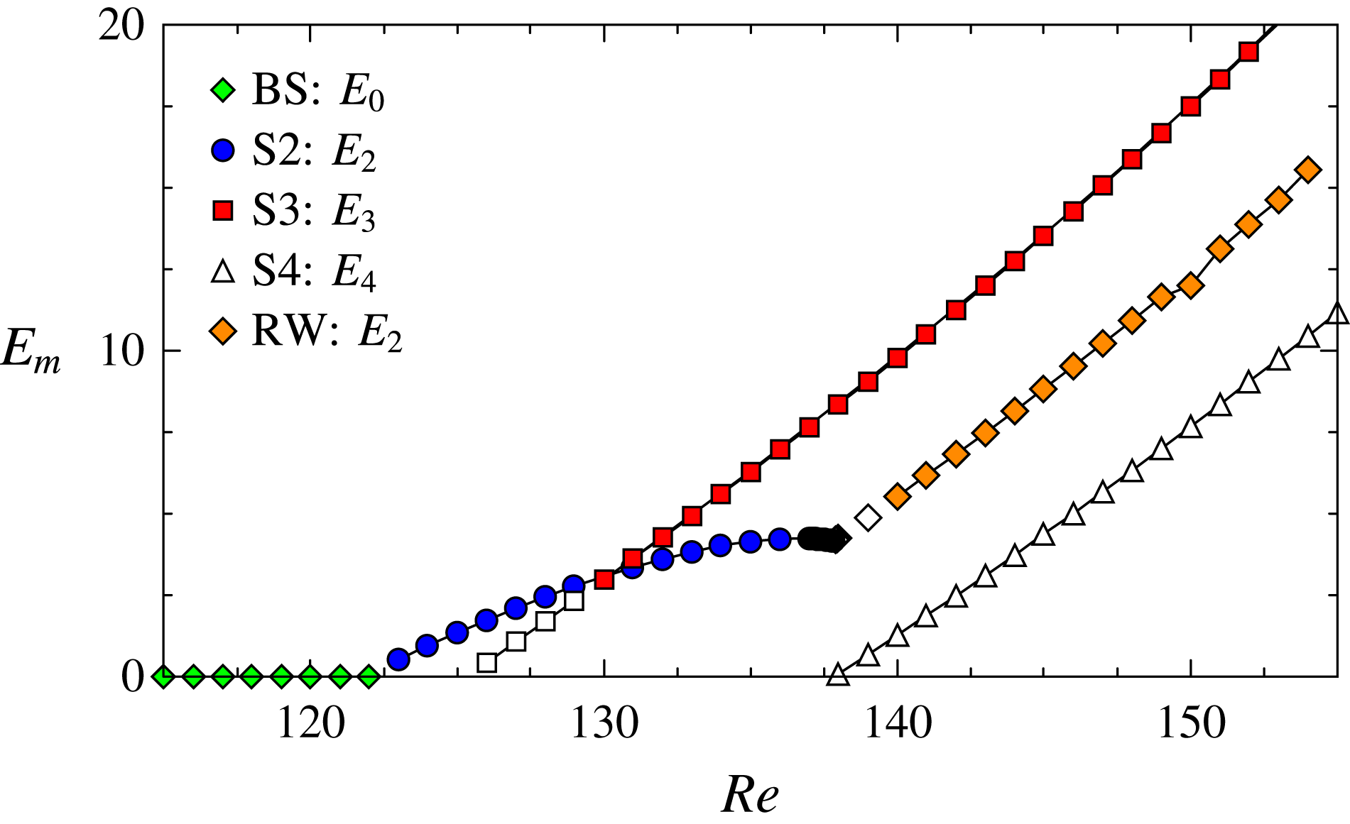
fixed, which provides a parameter sweep through the middle of the region organized by the pair of 2 : 3 codim-2 points shown in figure 6. Figure 7 provides a summary of the various states and their stability in terms of the modal energy in their primary azimuthal wave number. Filled symbols indicate stable states in the full space
 $\unicode[STIX]{x1D709}_{1}$
and open symbols indicate unstable states which were computed in their respective subspaces
 $\unicode[STIX]{x1D709}_{m}$
.
Variation of modal kinetic energies with
 $\mathit{Re}$
for various states as indicated, with
 $\unicode[STIX]{x1D6E4}=1.45$
. The unstable states (open symbols) were computed in their respective subspaces.

With
 $\unicode[STIX]{x1D6E4}=1.45$
fixed, BS is stable for
 $\mathit{Re}\lesssim 122.5$
. It becomes unstable for larger
 $\mathit{Re}$
via the circle-pitchfork spawning the circle of steady states S2. At
 $\mathit{Re}\approx 125.5$
, BS undergoes another circle-pitchfork bifurcation and spawns a circle of steady states S3, which are unstable since BS is also unstable. This bifurcation and the unstable S3 were computed in the subspace
 $\unicode[STIX]{x1D709}_{3}$
. At
 $\mathit{Re}\approx 129.5$
, the unstable S3 undergoes a bifurcation at which it is rendered stable. So far, all of these bifurcations were discussed in the context of figure 6, and are associated with the dynamics local to the 2 : 3 codim-2 points. As
 $\mathit{Re}$
approaches 138, a number of other events unfold. At
 $\mathit{Re}\approx 137.5$
, S2 becomes unstable. At slightly larger
 $\mathit{Re}$
, using S2 from slightly lower
 $\mathit{Re}$
as the initial condition, the flow evolves to the stable S3. However, restricting the flow to the
 $\unicode[STIX]{x1D709}_{2}$
subspace, S2 remains stable until
 $\mathit{Re}\approx 137.9$
, at which point it loses stability via a drift-pitchfork bifurcation (Coullet & Iooss Reference Coullet and Iooss1990; Crawford & Knobloch Reference Crawford and Knobloch1991; Fauve, Douady & Thual Reference Fauve, Douady and Thual1991; Kness, Tuckerman & Barkley Reference Kness, Tuckerman and Barkley1992) at which a rotating wave, RW, with azimuthal wavenumber
 $m=2$
is spawned. This RW will be described in detail in § 3.5. S2 continues to exist beyond the drift-pitchfork bifurcation but it is unstable, both in
 $\unicode[STIX]{x1D709}_{1}$
and
 $\unicode[STIX]{x1D709}_{2}$
, and we do not have a convenient way to compute it.
Also at
 $\mathit{Re}\approx 137.9$
, BS undergoes a third circle-pitchfork bifurcation creating an unstable S4 which we are able to compute in the
 $\unicode[STIX]{x1D709}_{4}$
subspace. We have continued the S4 branch in
 $\unicode[STIX]{x1D709}_{4}$
to
 $\mathit{Re}=200$
. Note that S2 and S3 do not exist in
 $\unicode[STIX]{x1D709}_{4}$
. In
 $\unicode[STIX]{x1D709}_{4}$
, S4 is stable until it loses stability at
 $\mathit{Re}\approx 161.5$
in a supercritical Hopf bifurcation that breaks the
 ${\mathcal{H}}_{\unicode[STIX]{x1D6FE}}$
symmetry of S4, spawning a direction-reversing wave (Landsberg & Knobloch Reference Landsberg and Knobloch1991). This DRW will be described in detail in § 3.6.
3.5 Rotating wave RW from a drift-pitchfork bifurcation
As mentioned above, the drift-pitchfork bifurcation takes place in
 $\unicode[STIX]{x1D709}_{2}$
as S2 is unstable in the full space
 $\unicode[STIX]{x1D709}_{1}$
. A distinct characteristic of the drift-pitchfork bifurcation is that it breaks the
 ${\mathcal{H}}_{\unicode[STIX]{x1D6FE}}$
symmetry. Like the S2 from which they bifurcate, RW have broken rotational invariance
 ${\mathcal{R}}_{\unicode[STIX]{x1D6FC}}$
(for arbitrary
 $\unicode[STIX]{x1D6FC}$
, except
 $\unicode[STIX]{x1D6FC}=\unicode[STIX]{x03C0}$
), and since
 ${\mathcal{H}}_{\unicode[STIX]{x1D6FE}}$
is also broken, they drift slowly in
 $\unicode[STIX]{x1D703}$
near onset. Since the
 ${\mathcal{H}}_{\unicode[STIX]{x1D6FE}}$
symmetry is broken, these rotating waves come in counter-rotating pairs; one is obtained by applying
 ${\mathcal{H}}_{\unicode[STIX]{x1D6FE}}$
to the other, and which one is realized depends on initial conditions. The drift speed is zero at the bifurcation at
 $\mathit{Re}=\mathit{Re}_{c}$
, and it grows as
 $\sqrt{|\mathit{Re }-\mathit{ Re }_{c}|}$
. A typical RW at
 $(\unicode[STIX]{x1D6E4},\mathit{Re})=(1.45,142)$
is shown in figure 8. The broken
 ${\mathcal{H}}_{\unicode[STIX]{x1D6FE}}$
symmetry is most clearly detected in the contour plot of
 $w$
at the mid-plane, which has no straight
 $w=0$
contour through the centre of the cylinder (compare with the
 $w(z=0)$
contour plot for S2 in figure 5, which has two such lines through the centre).
Isosurfaces of (a)
 $w$
, (b)
 $w{-}w_{0}$
and (c) contours of
 $w$
at
 $z=0$
, for RW at
 $(\unicode[STIX]{x1D6E4},\mathit{Re})=(1.45,142)$
. See the online movie 1 available at https://doi.org/10.1017/jfm.2017.103 for an animation of
 $w{-}w_{0}$
.

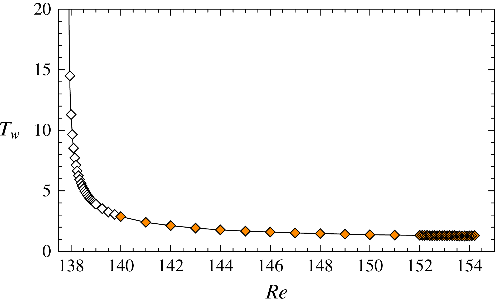
Drift period of RW,
 $T_{w}$
, versus
 $\mathit{Re}$
, together with a curve fit
 $T_{w}=0.117+4.018/\sqrt{\mathit{Re }-137.872}$
. The unstable RW (open symbols) were computed in
 $\unicode[STIX]{x1D709}_{2}$
.

Since rotating waves simply drift at a constant speed without change of shape (see the associated online movie 1), their modal kinetic energies are time invariant, but a point-wise measure (a velocity component at some point) has a periodic signal. The period of such a signal,
 $T_{w}$
, for RW as a function of
 $\mathit{Re}$
is shown in figure 9. The open symbols correspond to RW computed in
 $\unicode[STIX]{x1D709}_{2}$
and the filled symbols correspond to RW computed in the full space
 $\unicode[STIX]{x1D709}_{1}$
. The curve fit is
 $T_{w}=0.117+4.018/\sqrt{\mathit{Re }-137.872}$
, indicating that the drift-pitchfork bifurcation happens at
 $\mathit{Re}\approx 137.872$
. In summary, the RW have the invariances
 ${\mathcal{R}}_{\unicode[STIX]{x03C0}}\boldsymbol{u}=\boldsymbol{u}$
,
 ${\mathcal{R}}_{\unicode[STIX]{x1D6FC}}\boldsymbol{u}={\mathcal{T}}_{(\unicode[STIX]{x1D6FC}T_{w})/2\unicode[STIX]{x03C0}}\boldsymbol{u}$
for arbitrary
 $\unicode[STIX]{x1D6FC}$
, and
 ${\mathcal{T}}_{T_{w}}\boldsymbol{u}=\boldsymbol{u}$
.
At
 $\mathit{Re}\approx 139.8$
, the unstable RW undergoes a bifurcation in
 $\unicode[STIX]{x1D709}_{1}$
that renders it stable for larger
 $\mathit{Re}$
. What is spawned at this bifurcation is unstable and we do not have any direct information to determine its features, but the bifurcation must be of subcritical symmetry-breaking type as RW in
 $\unicode[STIX]{x1D709}_{2}$
does not change stability type in this range of
 $\mathit{Re}$
. RW remains stable up to
 $\mathit{Re}\approx 154.1$
; simulations at slightly larger
 $\mathit{Re}$
using RW at slightly lower
 $\mathit{Re}$
as the initial condition evolve to a different time-dependent state that has very different spatio-temporal characteristics compared to RW. We call this new state a pulse wave PWs, for reasons that will become evident when we describe it in § 3.7.
3.6 Direction-reversing wave from a Hopf bifurcation
We now turn our attention to
 $\unicode[STIX]{x1D709}_{4}$
and S4 that bifurcates from BS at
 $\mathit{Re}\approx 137.9$
. S4 loses stability in
 $\unicode[STIX]{x1D709}_{4}$
at
 $\mathit{Re}\approx 161.5$
in a supercritical Hopf bifurcation that breaks the
 ${\mathcal{H}}_{\unicode[STIX]{x1D6FE}}$
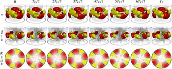
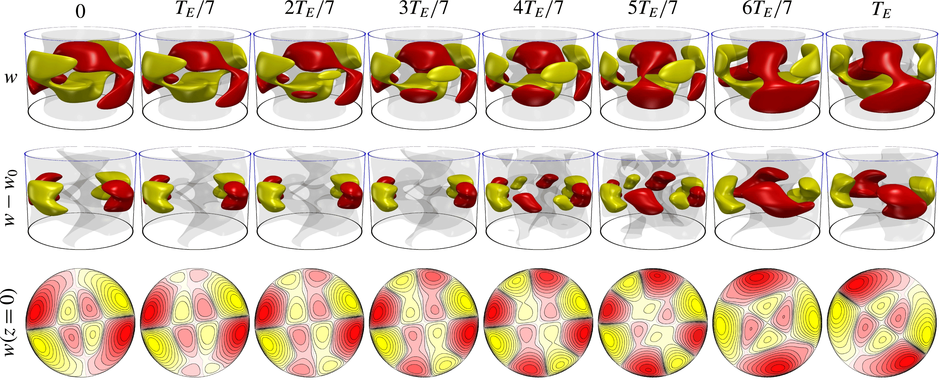
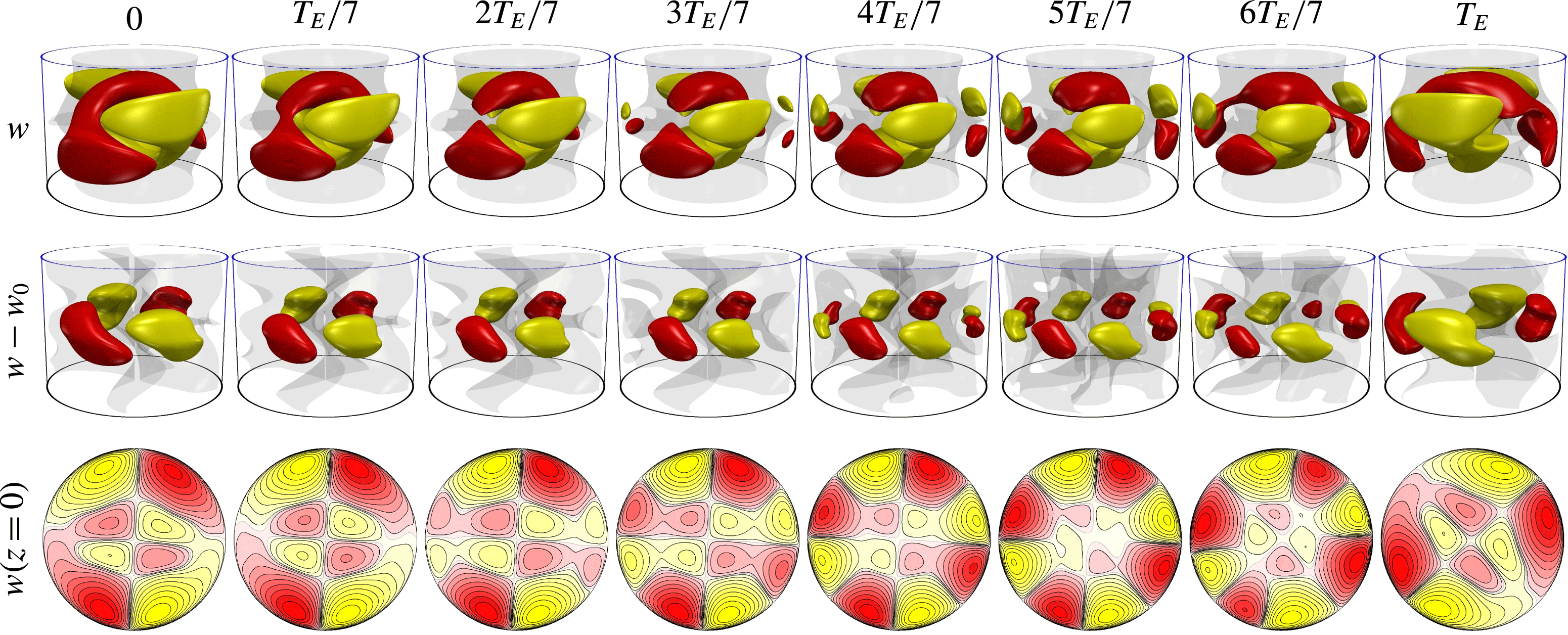
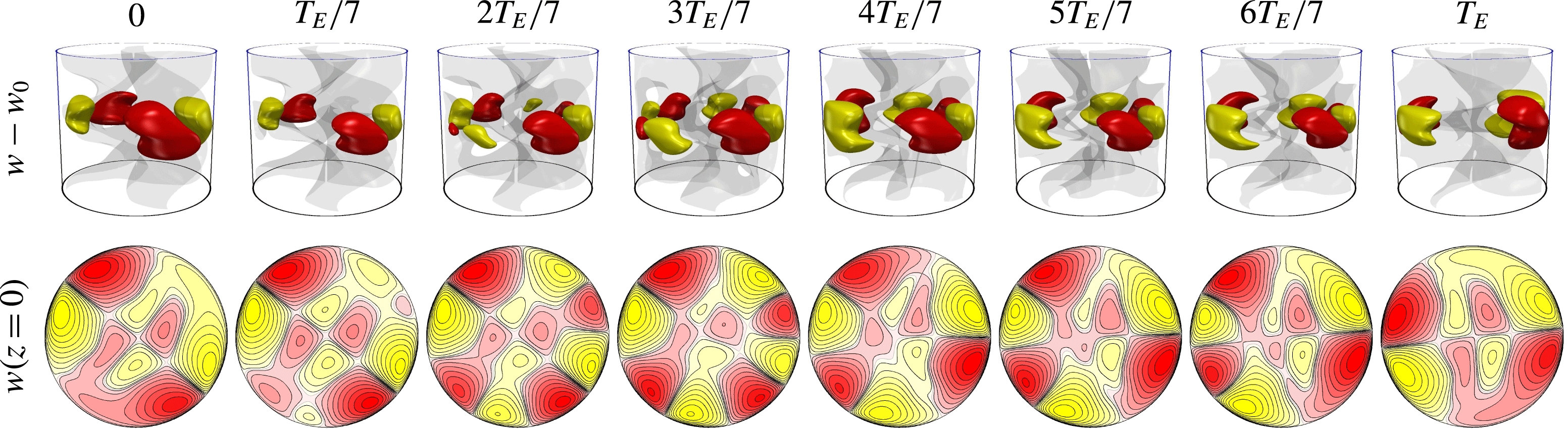
symmetry. Figure 10 shows snap-shots over one period of the direction-reversing wave DRW at
 $(\unicode[STIX]{x1D6E4},\mathit{Re})=(1.45,165)$
, and the accompanying movie 2 animates the
 $w{-}w_{0}$
isosurfaces for this case, illustrating how the structure oscillates back and forth in the azimuthal direction with a swelling and deflation of the structure in a period
 $T_{E}$
(the period of the modal kinetic energy variation). The key ingredient necessary for a direction-reversing wave is a Hopf bifurcation that breaks the reflection symmetry of a circle of non-trivial steady states, in our case these are S4 (Landsberg & Knobloch Reference Landsberg and Knobloch1991). The breaking of the
 ${\mathcal{H}}_{\unicode[STIX]{x1D6FE}}$
symmetry is most clearly seen by comparing the
 $w(z=0)$
contour plots of DRW in figure 10 with those of S4 in figure 5, which is
 ${\mathcal{H}}$
-symmetric about four lines through the axis.
Snapshots over one
 $T_{E}$
period relative to an arbitrary reference time of
 $w$
-isosurfaces,
 $w{-}w_{0}$
-isosurfaces and
 $w$
contours at
 $z=0$
for DRW at
 $(\unicode[STIX]{x1D6E4},\mathit{Re})=(1.45,165)$
computed in
 $\unicode[STIX]{x1D709}_{4}$
. See the online movie 2 for an animation of
 $w{-}w_{0}$
.

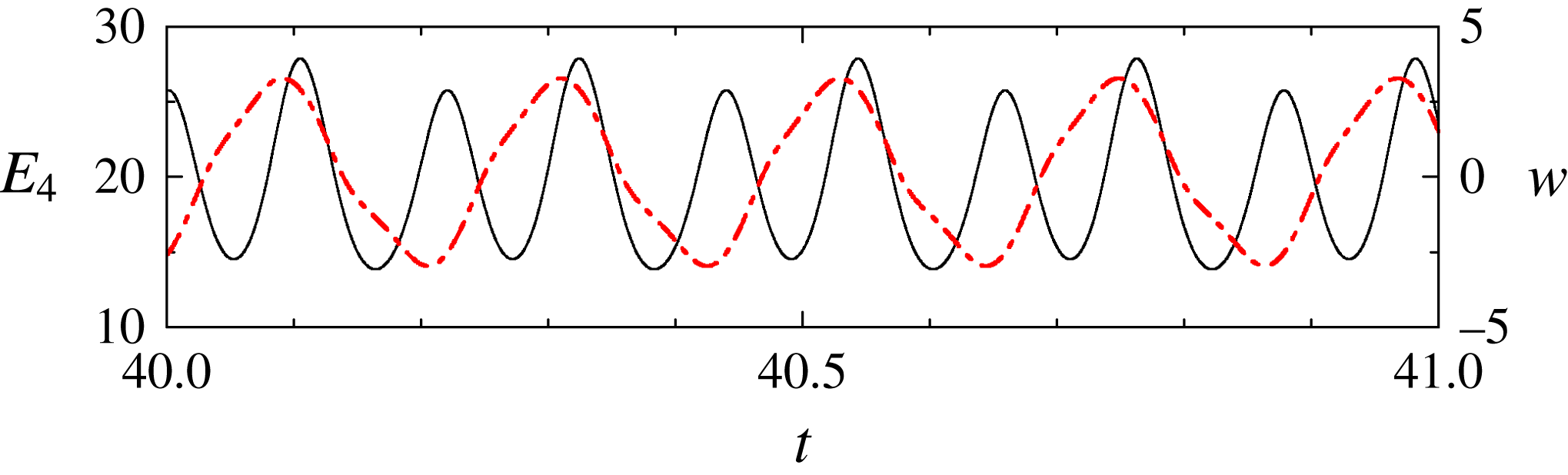
Time series of
 $E_{4}$
(solid line) and
 $w(0.98,0,-0.4\unicode[STIX]{x1D6E4})$
(dashed line) of DRW at
 $(\unicode[STIX]{x1D6E4},\mathit{Re})=(1.45,165)$
, computed in
 $\unicode[STIX]{x1D709}_{4}$
.

(a) Peak-to-peak amplitude and (b) period of
 $E_{4}$
for DRW at
 $\unicode[STIX]{x1D6E4}=1.45$
, computed in
 $\unicode[STIX]{x1D709}_{4}$
. The stable S4 are indicated as (blue) diamonds in order to show the region of hysteresis between S4 and DRW.

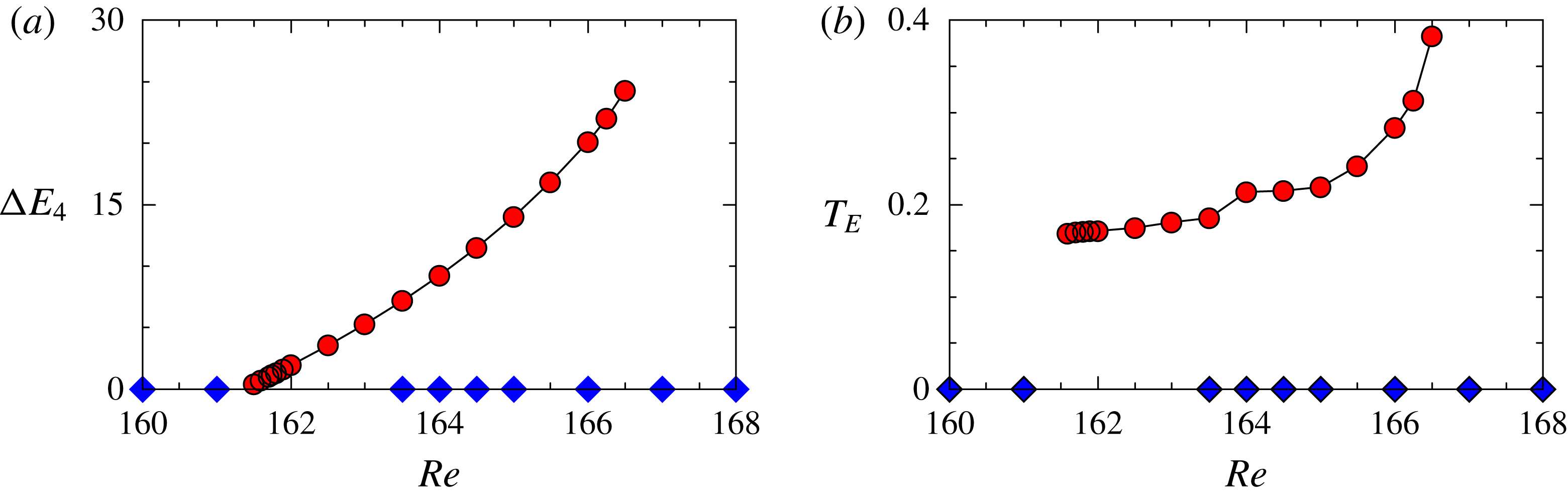
Unlike RW which have constant modal kinetic energies, the modal kinetic energies of DRW are time periodic. Their frequency is associated with the Hopf frequency at the bifurcation and the peak-to-peak amplitude in the modal kinetic energies grow linearly from zero with
 $|\mathit{Re}-\mathit{Re}_{c}|$
, for
 $\mathit{Re}\sim \mathit{Re}_{c}$
. Figure 11 shows time series of modal kinetic energy
 $E_{4}$
and of
 $w(0.98,0,-0.4\unicode[STIX]{x1D6E4})$
for DRW at
 $(\unicode[STIX]{x1D6E4},\mathit{Re})=(1.45,165)$
; both are periodic with period
 $T_{E}$
. Figure 12 shows the variations with
 $\mathit{Re}$
of the peak-to-peak amplitude and period of
 $E_{4}$
for DRW. Near the bifurcation at
 $\mathit{Re}\approx 161.5$
, the behaviour of the amplitude and period is typical of a supercritical Hopf bifurcation (Strogratz Reference Strogratz1994). DRW loses stability at
 $\mathit{Re}\approx 166.5$
in what is most likely a cyclic-fold bifurcation (saddle-node bifurcation of limit cycles), and S4 is stable for larger
 $\mathit{Re}$
. We have continued S4 in
 $\unicode[STIX]{x1D709}_{4}$
up to
 $\mathit{Re}=200$
. Also, we have continued S4 to lower
 $\mathit{Re}$
, and find that it becomes unstable at
 $\mathit{Re}\approx 163.5$
where is undergoes a subcritical Hopf spawning an unstable DRW to higher
 $\mathit{Re}$
which is involved in the cyclic-fold bifurcation at
 $\mathit{Re}\approx 166.5$
.
The fundamental difference between RW and DRW is that while both result from bifurcations of
 $\text{S}m$
that break
 ${\mathcal{H}}_{\unicode[STIX]{x1D6FE}}$
(S2 for RW and S4 for DRW), the bifurcation leading to RW is steady (real eigenvalue crosses zero) while that leading to DRW is not (the real part of a complex-conjugate pair of eigenvalues changes sign), so for RW the phase change is constant whereas for DRW it is periodic (Landsberg & Knobloch Reference Landsberg and Knobloch1991). In summary, the DRW have the invariances
 ${\mathcal{R}}_{\unicode[STIX]{x03C0}/2}\boldsymbol{u}=\boldsymbol{u}$
and
 ${\mathcal{T}}_{T_{E}}\boldsymbol{u}=\boldsymbol{u}$
.
3.7 Pulse waves
Attempts to continue RW beyond
 $\mathit{Re}\approx 154.1$
in
 $\unicode[STIX]{x1D709}_{2}$
result in the same evolutions as in
 $\unicode[STIX]{x1D709}_{1}$
, indicating that RW ceases to exist beyond
 $\mathit{Re}\approx 154.1$
due to a cyclic-fold bifurcation. For
 $\mathit{Re}$
beyond this bifurcation, we find pulse wave states PWs. Like RW, PWs are invariant to
 ${\mathcal{R}}_{\unicode[STIX]{x03C0}}$
, i.e. they reside in
 $\unicode[STIX]{x1D709}_{2}$
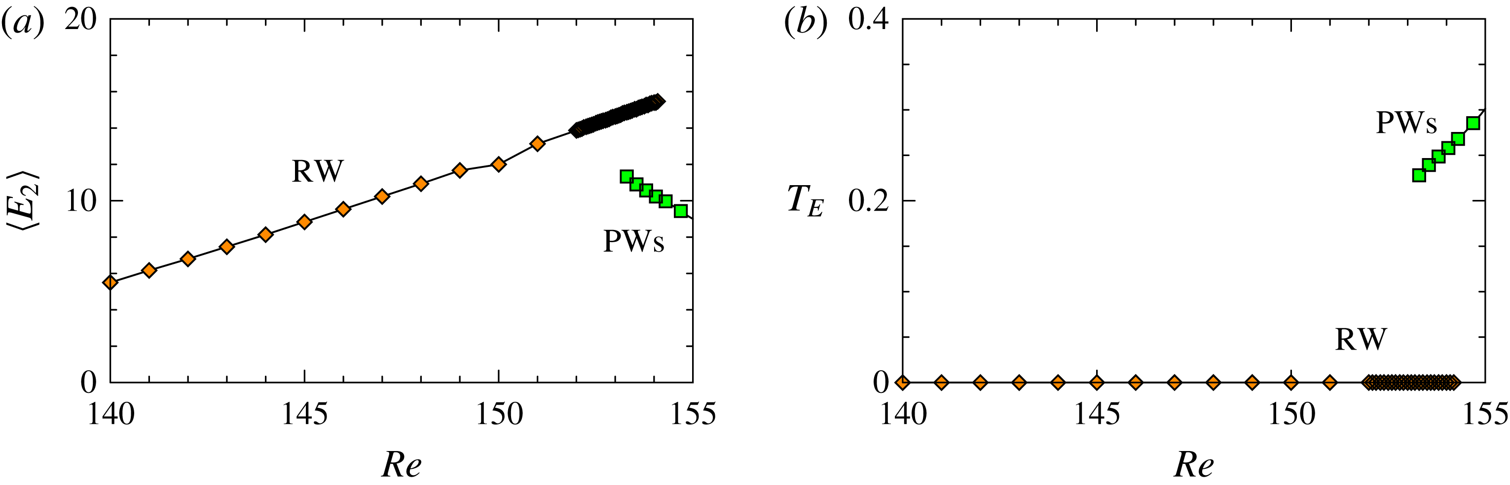
. The PWs are stable to lower
 $\mathit{Re}\approx 153.3$
, below which they are destroyed, presumably also in a cyclic-fold bifurcation, so that we have a region of hysteresis between RW and PWs over
 $\mathit{Re}\in (153.3,154.1)$
.
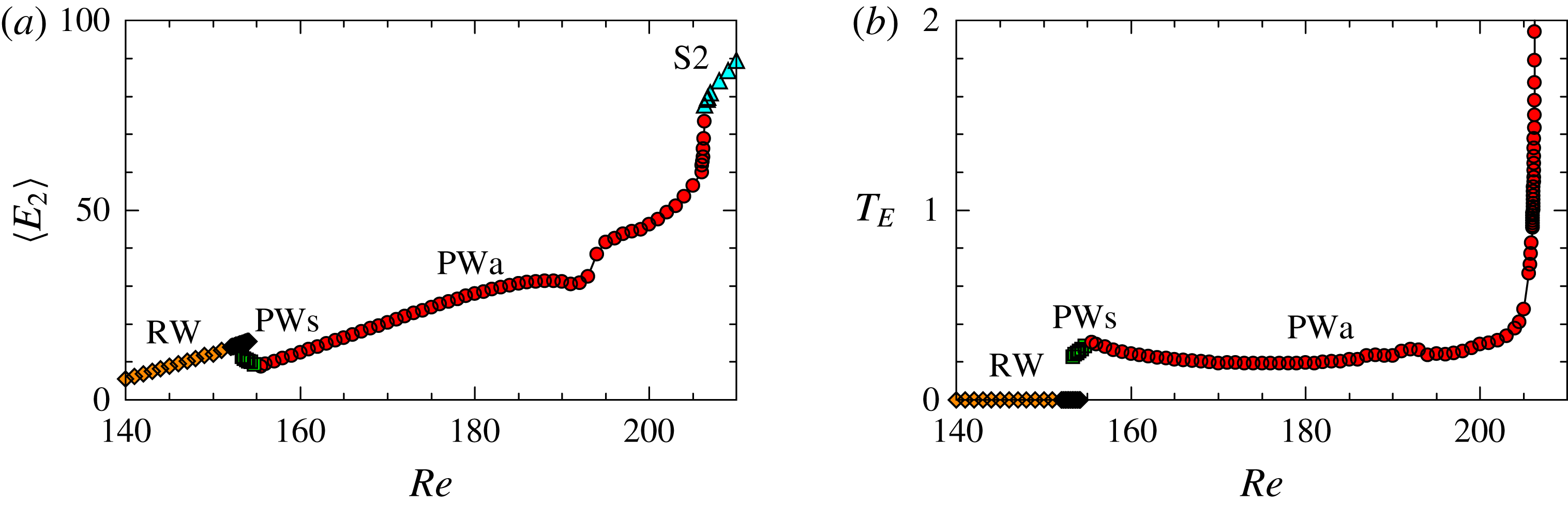
Variation with
 $\mathit{Re}$
of (a) the time-averaged modal energy
 $\langle E_{2}\rangle$
and (b) the period
 $T_{E}$
of RW and PWs, for
 $\unicode[STIX]{x1D6E4}=1.45$
, computed in the full space
 $\unicode[STIX]{x1D709}_{1}$
.

Figure 13(a) shows the time-averaged modal kinetic energy
 $\langle E_{2}\rangle$
for RW and PWs over their hysteresis region in
 $\mathit{Re}$
. Note that
 $\langle E_{2}\rangle =E_{2}$
for RW. Figure 13(b) shows the corresponding energy period,
 $T_{E}$
, of oscillation in
 $E_{2}$
. For RW,
 $T_{E}=0$
since the solution is only rotating, uniformly changing its azimuthal orientation, but not changing its structure.
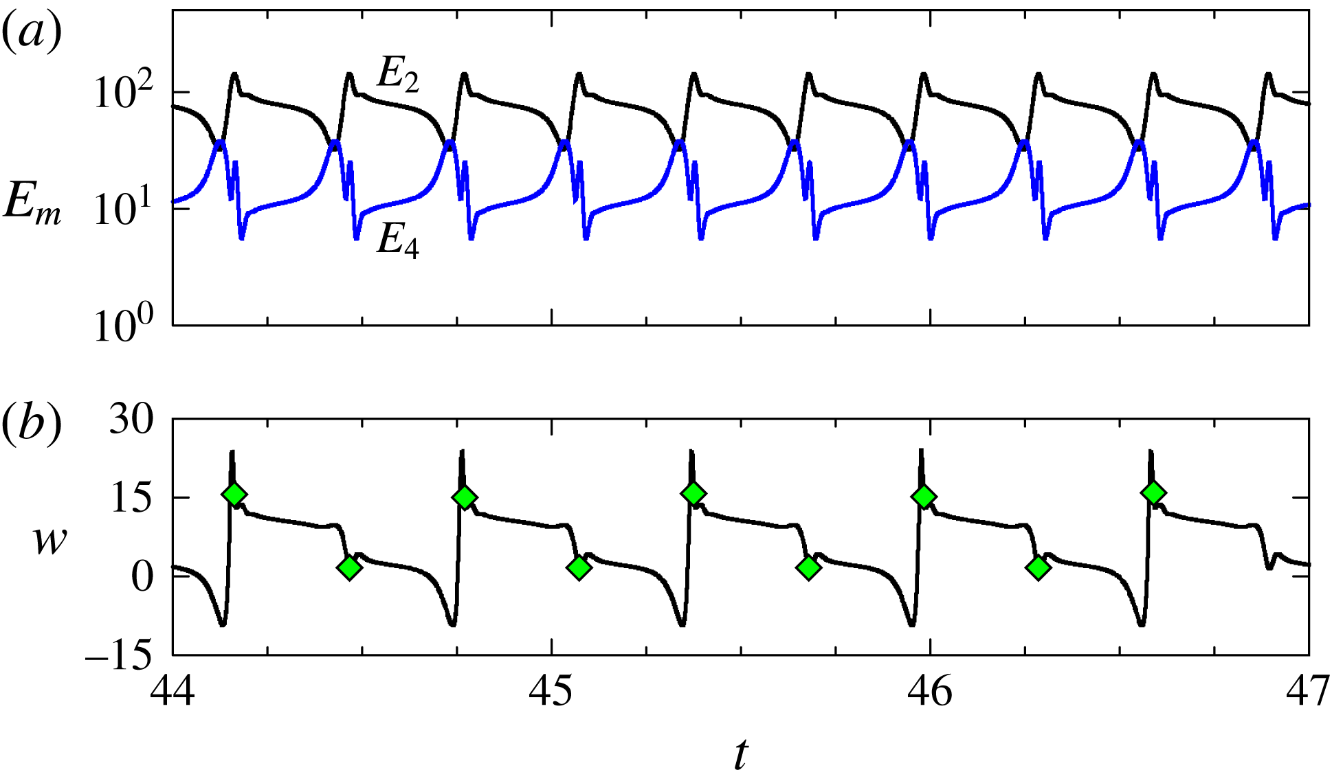
Time series of (a) modal kinetic energies
 $E_{2}$
and
 $E_{4}$
, and (b)
 $w(0.98,0,-0.4\unicode[STIX]{x1D6E4})$
for PWs at
 $(\unicode[STIX]{x1D6E4},\mathit{Re})=(1.45,153.5)$
. The (green) diamonds correspond to the numbered diamonds in figure 16.

Snapshots over one
 $T_{E}$
period relative to an arbitrary reference time of
 $w$
-isosurfaces,
 $w{-}w_{0}$
-isosurfaces and
 $w$
contours at
 $z=0$
for PWs at
 $(\unicode[STIX]{x1D6E4},\mathit{Re})=(1.45,153.5)$
. See the online movie 3 for an animation of
 $w{-}w_{0}$
.

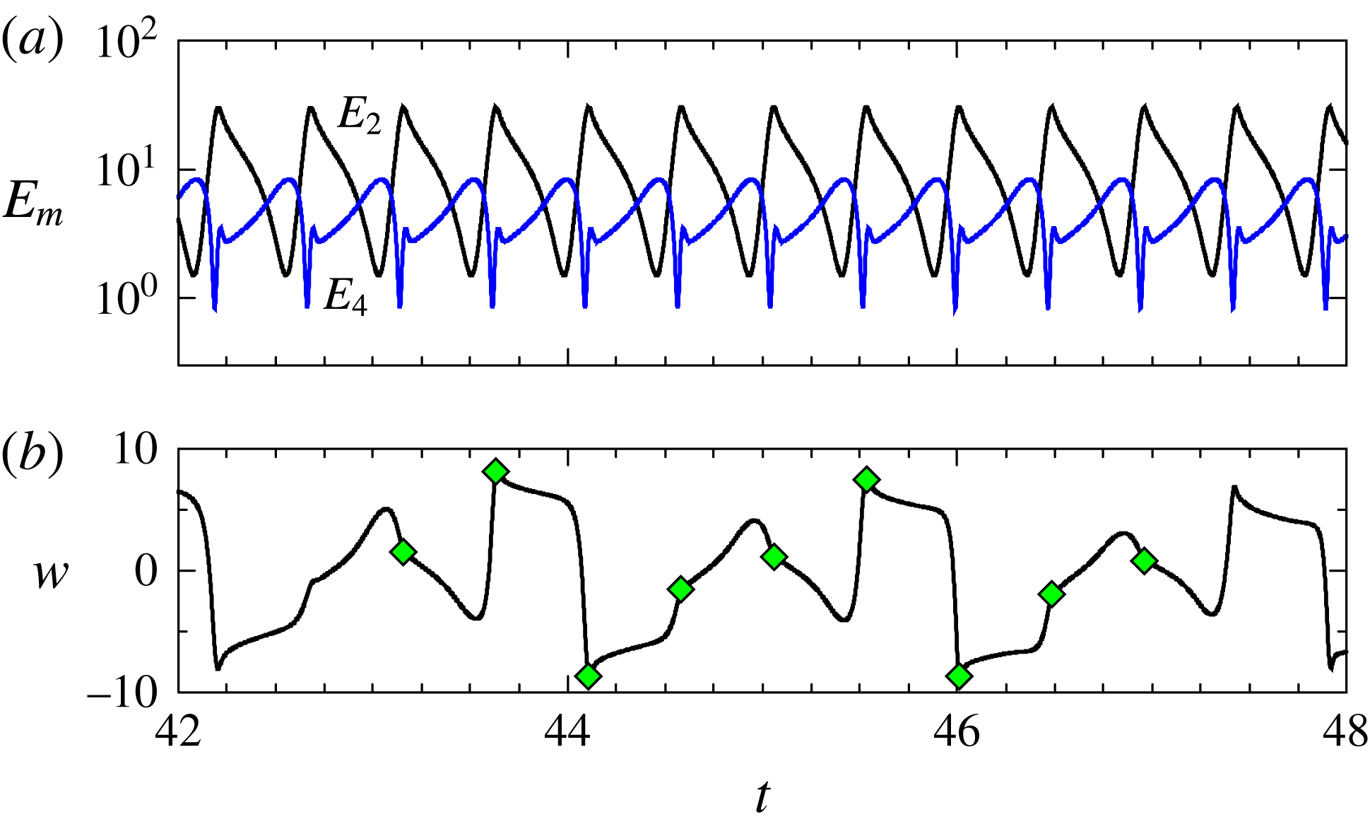
PWs is an unsteady flow with slow–fast dynamics, as can be seen from the time series of
 $E_{2}$
and
 $E_{4}$
shown in figure 14(a). The fast dynamics consists of a rapid growth in
 $E_{2}$
; when
 $E_{2}$
reaches its maximum,
 $E_{4}$
begins to grow and
 $E_{2}$
slowly decays, then the cycle repeats. The dynamics is easiest to visualize from isosurfaces of
 $w{-}w_{0}$
. Figure 15 for PWs at
 $\mathit{Re}=153.5$
shows snap-shots of
 $w$
and
 $w{-}w_{0}$
isosurfaces and
 $w$
contours at the mid-plane over one
 $T_{E}$
period (the associated online movie 3 animates the
 $w{-}w_{0}$
isosurfaces over
 $8T_{E}$
to better illustrate the slow–fast dynamics). The steady state S2 has two pairs of oppositely signed blobs of
 $w{-}w_{0}$
symmetrically distributed in azimuth about the mid-plane. In the slow phase of PWs, there are also two pairs of oppositely signed blobs of
 $w{-}w_{0}$
. These blobs slowly diminish in size and the oppositely signed blobs in each pair slowly approach each other. In so doing, two increasingly wide swaths with near-zero
 $w{-}w_{0}$
result about the mid-plane. Then, during the fast phase of the oscillation, two new pairs of blobs appear in the near-zero swaths between the two existing pairs. When the new blobs are comparable to the pre-existing blobs, the positive new blobs and the negative old blobs move toward each other and the other blobs vanish, leaving a configuration that again closely resembles the S2 steady state, but rotated by approximately
 $\unicode[STIX]{x03C0}/4$
with respect to the earlier orientation. This occurs in one period
 $T_{E}$
and the original orientation is almost regained in about
 $8T_{E}$
.
Phase portraits, (a) using
 $w(0.98,0,0,t)$
and
 $w(0.98,0,0.2\unicode[STIX]{x1D6E4},t)$
and (b) using
 $E_{2}$
and
 $E_{4}$
, for PWs at
 $(\unicode[STIX]{x1D6E4},\mathit{Re})=(1.45,153.5)$
; there are 25 equispaced-in-time circular markers over
 $T_{E}$
.

Although the time series of the modal kinetic energies of PWs are
 $T_{E}$
-periodic, PWs are not time periodic. This is evident from the time series of
 $w(0.98,0,-0.4\unicode[STIX]{x1D6E4})$
, shown in figure 14(b); the (green) diamonds in the figure are equispaced every
 $T_{E}$
and correspond to maxima in
 $E_{2}$
. What happens is that in exactly one period
 $T_{E}$
, the structure of PWs is the same as its structure a period earlier, and hence has the same modal kinetic energies, but its orientation has changed by almost
 $\unicode[STIX]{x03C0}/4$
, and so the local measure of
 $w$
is different. If the orientation had changed by exactly
 $\unicode[STIX]{x03C0}/4$
(or some other rational fraction of
 $\unicode[STIX]{x03C0}$
), the
 $w$
signal would also be periodic, but this does not happen generically. Figure 16(a) shows a phase portrait of PWs at
 $(\unicode[STIX]{x1D6E4},\mathit{Re})=(1.45,153.5)$
, using
 $w(0.98,0,0)$
and
 $w(0.98,0,0.2\unicode[STIX]{x1D6E4})$
, over many
 $T_{E}$
, showing the structure of a 2-torus in grey. The line in black is a part of the trajectory over
 $8T_{E}$
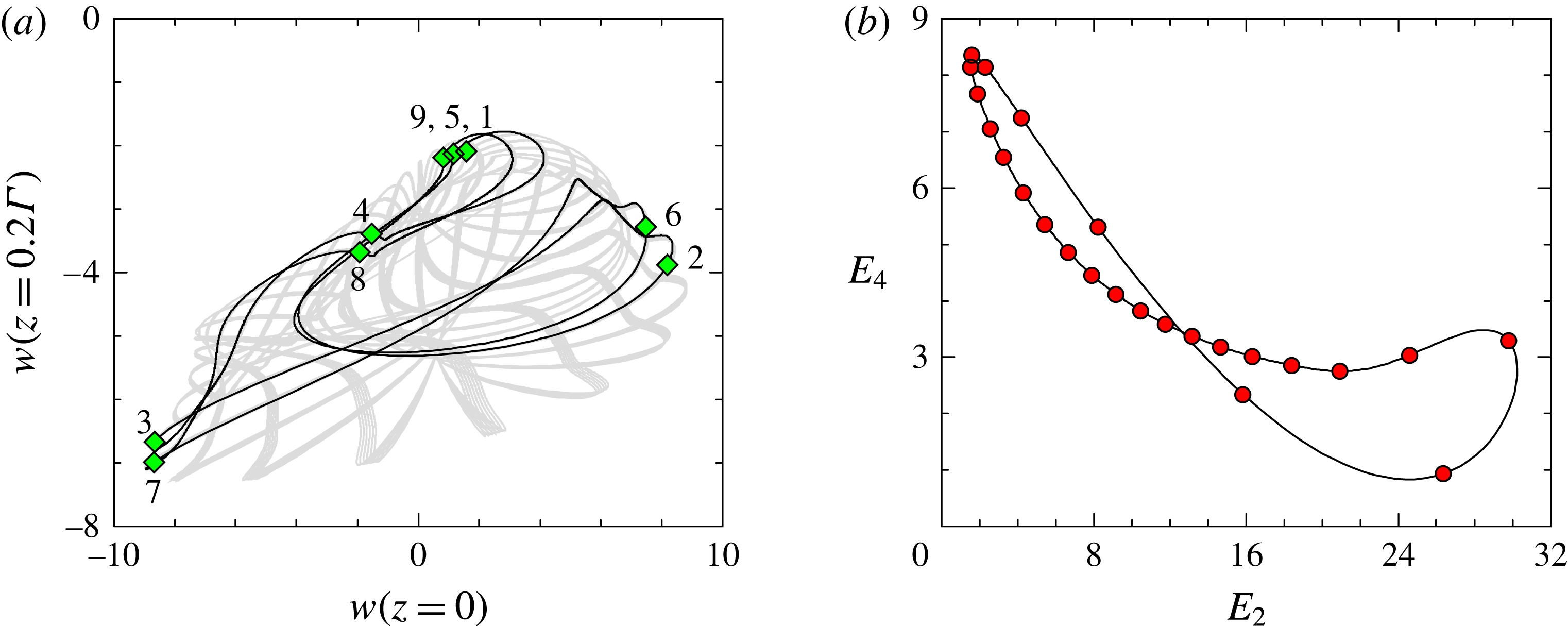
and the (green) diamonds correspond to the same symbols in the corresponding time series in figure 14. The trajectory is almost a cycle that closes in on itself. However, it does not; the symbol labelled 9 does not coincide with that labelled 1, and the trajectory eventually covers the torus. Such states are sometimes referred to as relative periodic orbits, states that would appear to be periodic if viewed from a reference frame rotating at the angular rate corresponding to the angular change in orientation every
 $T_{E}$
period. This is in the same sense that rotating waves are relative equilibria, states that would appear steady when viewed from a reference frame rotating at the angular rotation rate of the rotating wave. In figure 16(b), a phase portrait of the same PWs is shown using
 $E_{2}$
and
 $E_{4}$
. This is a closed cycle, as expected. The symbols on the closed curve correspond to 25 uniformly spaced times over
 $T_{E}$
, to show the slow–fast character of the oscillation.
In summary, the PWs have the invariances
 ${\mathcal{R}}_{\unicode[STIX]{x03C0}}\boldsymbol{u}=\boldsymbol{u}$
and
 ${\mathcal{R}}_{\unicode[STIX]{x1D6FC}}\boldsymbol{u}={\mathcal{T}}_{T_{E}}\boldsymbol{u}$
for some
 $\unicode[STIX]{x1D6FC}$
that is not a rational fraction of
 $\unicode[STIX]{x03C0}$
.
3.8 Symmetry breaking to PWa
The pulse wave PWs is stable in
 $\unicode[STIX]{x1D709}_{1}$
, but resides in
 $\unicode[STIX]{x1D709}_{2}$
since all of its odd azimuthal Fourier components have zero modal kinetic energy. PWs is stable up to
 $\mathit{Re}\approx 155.15$
, where it loses stability in a supercritical symmetry-breaking bifurcation breaking the
 ${\mathcal{R}}_{\unicode[STIX]{x03C0}}$
rotational invariance. The state that is spawned is referred to as PWa. The bifurcation results in the
 $m=3$
Fourier component being excited, and so PWa resides in the full space
 $\unicode[STIX]{x1D709}_{1}$
. Like PWs, PWa has slow–fast dynamics, and for the most part looks very much like PWs, spending most of the time very close to the
 $\unicode[STIX]{x1D709}_{2}$
subspace, with a quick excursion out of it when
 $E_{3}$
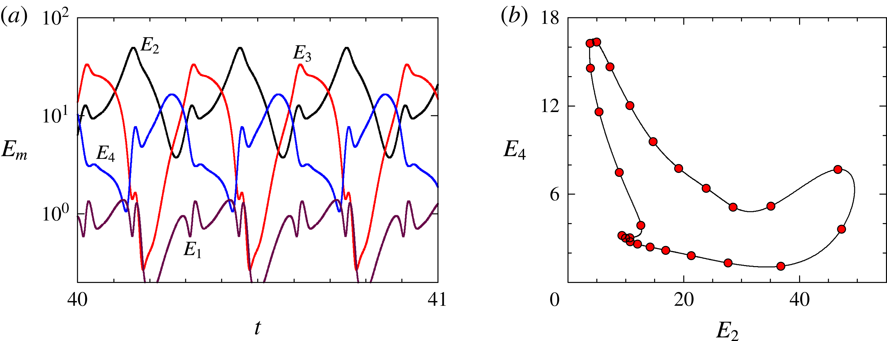
is large. Figure 17 shows snap-shots of
 $w$
and
 $w{-}w_{0}$
isosurfaces and
 $w$
contours at the mid-plane over one
 $T_{E}$
period for PWa at
 $(\unicode[STIX]{x1D6E4},\mathit{Re})=(1.45,160)$
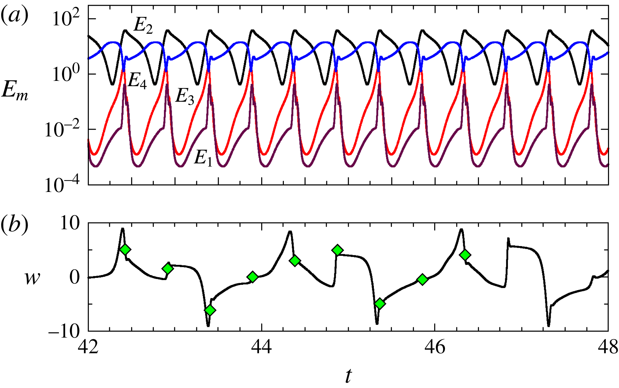
. They are not very different from the corresponding images for PWs shown in figure 15. The phase portraits of PWa in figure 18 are also qualitatively the same as those for PWs shown in figure 16. However, the time series of
 $E_{1}$
,
 $E_{2}$
,
 $E_{3}$
,
 $E_{4}$
and
 $w$
in figure 19 clearly show how
 $E_{3}$
comes into play in the slow–fast dynamics.
 $E_{1}$
is smaller than and slaved to
 $E_{3}$
, and comes about via the nonlinear interaction between
 $E_{3}$
with
 $E_{2}$
and
 $E_{4}$
. Note that the
 $E_{m}$
time series are also strictly
 $T_{E}$
periodic, as for PWs. For both PWs and PWa, in exactly one period
 $T_{E}$
, their structure is the same as it was a period earlier, and hence they have the same modal kinetic energies as they did one period earlier, but their orientation has changed, by almost
 $\unicode[STIX]{x03C0}/4$
. They are both relative periodic orbits.
Snapshots over one
 $T_{E}$
period relative to an arbitrary reference time of
 $w$
-isosurfaces,
 $w{-}w_{0}$
-isosurfaces and
 $w$
contours at
 $z=0$
for PWa at
 $(\unicode[STIX]{x1D6E4},\mathit{Re})=(1.45,160)$
computed in
 $\unicode[STIX]{x1D709}_{2}$
. See the online movie 4 for an animation of
 $w{-}w_{0}$
.

Phase portraits, (a) using
 $w(0.98,0,0,t)$
and
 $w(0.98,0,0.2\unicode[STIX]{x1D6E4},t)$
and (b) using
 $E_{2}$
and
 $E_{4}$
, for PWa at
 $(\unicode[STIX]{x1D6E4},\mathit{Re})=(1.45,160)$
; there are 25 equispaced-in-time circular markers over
 $T_{E}$
.

Time series of (a) modal kinetic energies
 $E_{1}$
,
 $E_{2}$
,
 $E_{3}$
and
 $E_{4}$
and (b)
 $w(0.98,0,-0.4\unicode[STIX]{x1D6E4})$
for PWa at
 $(\unicode[STIX]{x1D6E4},\mathit{Re})=(1.45,160)$
. The diamonds correspond to the numbered diamonds in figure 18.

The PWa have the invariance
 ${\mathcal{R}}_{\unicode[STIX]{x1D6FC}}\boldsymbol{u}={\mathcal{T}}_{T_{E}}\boldsymbol{u}$
for some
 $\unicode[STIX]{x1D6FC}$
that is not a rational fraction of
 $\unicode[STIX]{x03C0}$
.
3.9 Saddle-node-on-an-invariant-circle bifurcation destroying PWa
The period
 $T_{E}$
of PWa does not vary very much from its onset following the symmetry-breaking instability of PWs at
 $\mathit{Re}\approx 155.15$
to
 $\mathit{Re}\approx 200$
. As
 $\mathit{Re}$
is increased beyond 200,
 $T_{E}$
becomes increasing larger. Figure 20 shows how the amplitude (time-averaged
 $E_{2}$
) and period
 $T_{E}$
of RW, PWs and PWa vary with
 $\mathit{Re}$
. Each symbol in the figure corresponds to an individual simulation that was run for many viscous times to establish its time-asymptotic behaviour. For
 $\mathit{Re}>200$
, these simulations have been run for between 100 and 200 viscous times in order to accurately estimate the period
 $T_{E}$
. Over this
 $\mathit{Re}$
range,
 $T_{E}=0.285+0.831/\sqrt{206.312-\mathit{ Re}}$
is a very good fit to the computed period, and indicates that the period becomes unbounded at
 $\mathit{Re}=206.312$
.
Variation with
 $\mathit{Re}$
of (a) the time-averaged modal energy
 $\langle E_{2}\rangle$
and (b) the period
 $T_{E}$
of RW, PWs, PWa and S2 for
 $\unicode[STIX]{x1D6E4}=1.45$
, computed in the full space
 $\unicode[STIX]{x1D709}_{1}$
. Near
 $\mathit{Re}=206$
, the period of PWa has the fit
 $T_{E}=0.285+0.831/\sqrt{206.312-\mathit{ Re}}$
.

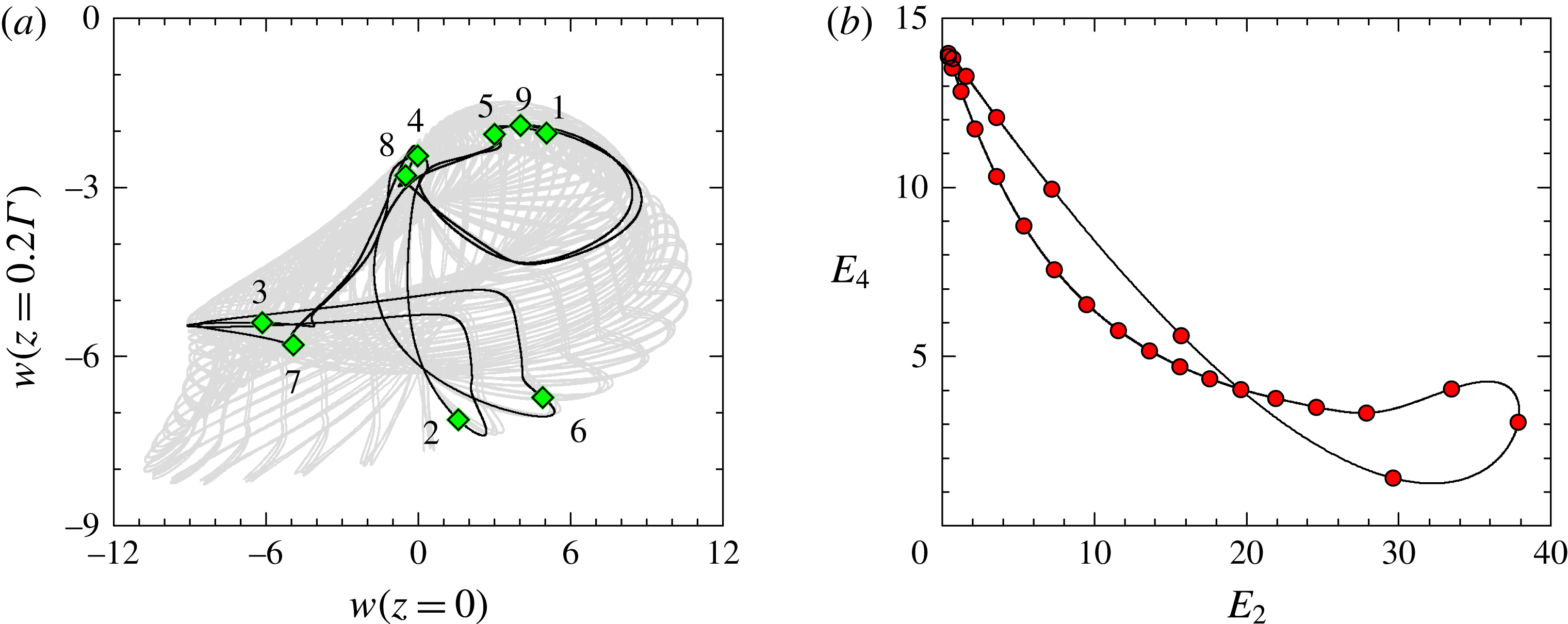
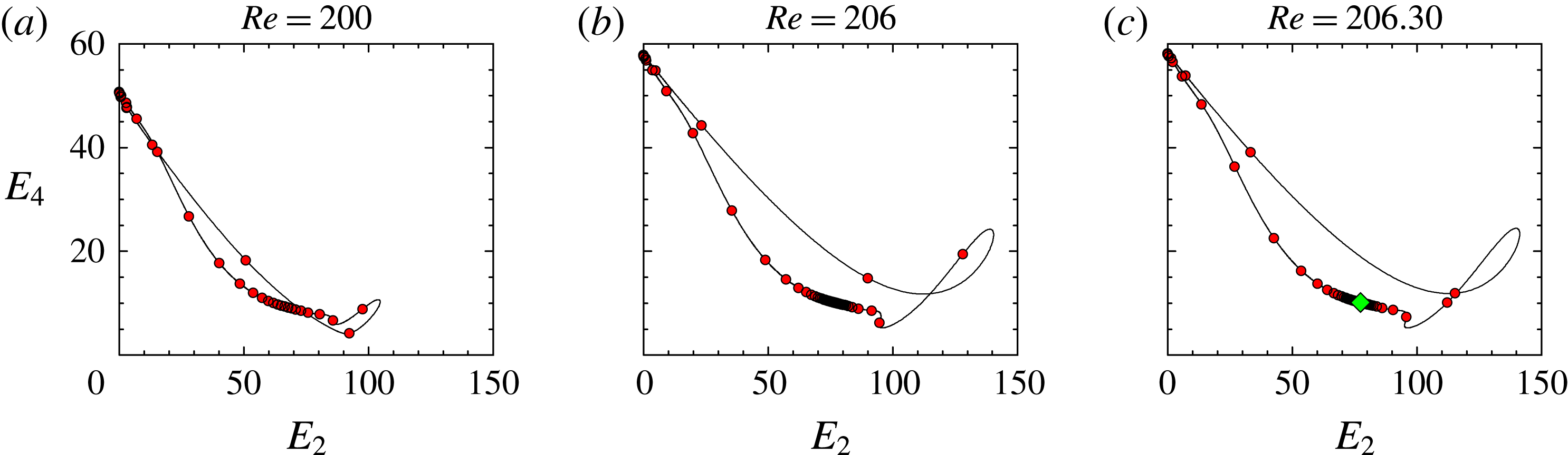
Phase portrait in
 $(E_{2},E_{4})$
for PWa at
 $\unicode[STIX]{x1D6E4}=1.45$
and
 $\mathit{Re}$
as indicated. There are 25 equispaced-in-time circular markers over
 $T_{E}$
, used to illustrate the slow–fast nonlinear oscillation. In (c), the (green) diamond corresponds to the steady S2 at
 $\mathit{Re}=206.32$
.

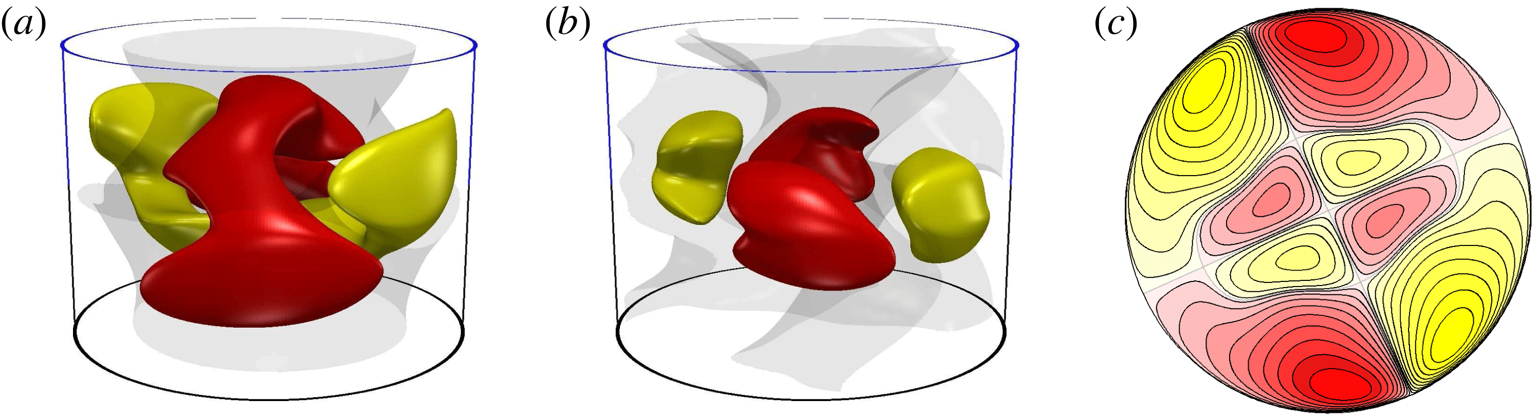
Isosurfaces of (a)
 $w$
, (b)
 $w{-}w_{0}$
and (c) contours of
 $w$
at
 $z=0$
, for S2 at
 $(\unicode[STIX]{x1D6E4},\mathit{Re})=(1.45,206.32)$
.

This inverse-square-root behaviour of the period dependence on
 $\mathit{Re}$
is typical of a SNIC bifurcation (a saddle-node-on-an-invariant-circle bifurcation). The slow–fast dynamics of PWa reaches a critical slowing down as
 $\mathit{Re}\rightarrow 206.312$
. This is illustrated in figure 21, showing phase portraits of PWa at three
 $\mathit{Re}$
approaching the critical value
 $\mathit{Re}=206.312$
. In the third portrait, corresponding to
 $\mathit{Re}=206.30$
, we find the (red) circles accumulate. On this same portrait we have included the
 $(E_{2},E_{4})$
point as a (green) diamond, corresponding to the stable steady state that is found following the SNIC bifurcation at
 $\mathit{Re}=206.32$
. This steady state is S2; its features are illustrated in figure 22. It has the same features as PWa during it slow phase (e.g. compare with the 0 phase of figure 17).
3.10 Behaviour over a broader range of parameter space
The one parameter sweep varying
 $\mathit{Re}$
while keeping
 $\unicode[STIX]{x1D6E4}=1.45$
revealed very rich dynamics and multiplicity of solutions, all associated with the manner in which the
 $O(2)$
symmetry is broken. In this section, we provide a broader overview considering variations in
 $\unicode[STIX]{x1D6E4}$
as well, although not in anywhere near as much detail. We have considered
 $\unicode[STIX]{x1D6E4}\in [0.5,2.0]$
in increments of 0.05, and used the BS at
 $\mathit{Re}=100$
for each of these
 $\unicode[STIX]{x1D6E4}$
as the initial conditions for larger
 $\mathit{Re}$
. For each
 $\unicode[STIX]{x1D6E4}$
, solutions with
 $\mathit{Re}$
up to 300, in increments of about 10 were computed until transients died off (up to a few dozen viscous time units). Some refinements in
 $\mathit{Re}$
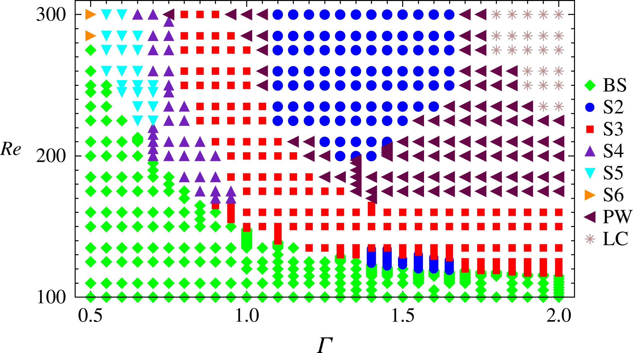
were done near the bifurcations for some of the cases. Figure 23 is a summary of the states computed using that process (about 800 simulations). Very close to the primary circle-pitchfork bifurcation curves, the corresponding
 $\text{S}m$
states are obtained. However, not too far after the circle-pitchfork bifurcations, the steady state S3 is obtained over a wide swath of parameter space. Then, the parameter space is dominated either by various types of pulse wave states (PWs and PWa, as well as others to be described below), or the S2 state that was found following the destruction of PWa via the SNIC bifurcation. Also, for a parameter region with
 $\unicode[STIX]{x1D6E4}\sim 2$
and
 $\mathit{Re}\sim 300$
, a limit cycle state without any non-trivial spatial symmetry (the invariance to
 ${\mathcal{R}}_{2\unicode[STIX]{x03C0}}$
is trivial), but with a space–time symmetry, exists (described below). Of course, there are multiplicities of solutions throughout the parameter space, and the manner in which we have solved the sequences of initial value problems does not bring any of that richness out (repeating the procedure used in the one parameter sweep at
 $\unicode[STIX]{x1D6E4}=1.45$
for the 30 other values of
 $\unicode[STIX]{x1D6E4}$
is beyond the scope of the present study). However, it does provide an indication of which solution types are likely to be found.
Loci of stable states in
 $(\unicode[STIX]{x1D6E4},\mathit{Re})$
, found by using BS at
 $\mathit{Re}=100$
at each
 $\unicode[STIX]{x1D6E4}$
as the initial condition for simulations for all
 $\mathit{Re}$
at that
 $\unicode[STIX]{x1D6E4}$
. No attempt was made to show loci of multiple stable states at the same point in parameter space that were found using other initial conditions.

Snapshots over one
 $T_{E}$
period, relative to an arbitrary reference time, of
 $w{-}w_{0}$
-isosurfaces and
 $w$
contours at
 $z=0$
for PWa at
 $(\unicode[STIX]{x1D6E4},\mathit{Re})=(1.80,175)$
. See the online movie 5 for an animation of
 $w{-}w_{0}$
.

(a) Time series of
 $E_{m}$
and (b) phase portrait using
 $E_{2}$
and
 $E_{4}$
for PWa at
 $(\unicode[STIX]{x1D6E4},\mathit{Re})=(1.80,175)$
.

We now address, to a very small degree, the changes in the pulse waves for different aspect ratios. In the parameter sweep varying
 $\mathit{Re}$
and keeping
 $\unicode[STIX]{x1D6E4}=1.45$
fixed, the level to which
 $E_{3}$
grows for PWa remains relatively small. However, by varying
 $\unicode[STIX]{x1D6E4}$
we have also found PWa in which
 $E_{3}$
is the dominant modal kinetic energy during a part of the oscillation. Figures 24 and 25 show snap-shots of
 $w{-}w_{0}$
isosurfaces and contour plots of
 $w$
at the mid-plane, as well as time series of the modal kinetic energies and a phase portrait of PWa at
 $(\unicode[STIX]{x1D6E4},\mathit{Re})=(1.80,175)$
. While the PWa is of the same type as described earlier at
 $(\unicode[STIX]{x1D6E4},\mathit{Re})=(1.45,160)$
, it has a very different apparent dynamic due to
 $E_{3}$
being dominant over some time intervals. This is easiest to visualize from the online movie 5 showing
 $w{-}w_{0}$
isosurface.
Time series of (a) modal kinetic energies
 $E_{2}$
and
 $E_{4}$
and (b)
 $w(0.98,0,-0.4\unicode[STIX]{x1D6E4})$
for PWo at
 $(\unicode[STIX]{x1D6E4},\mathit{Re})=(1.5,210)$
.

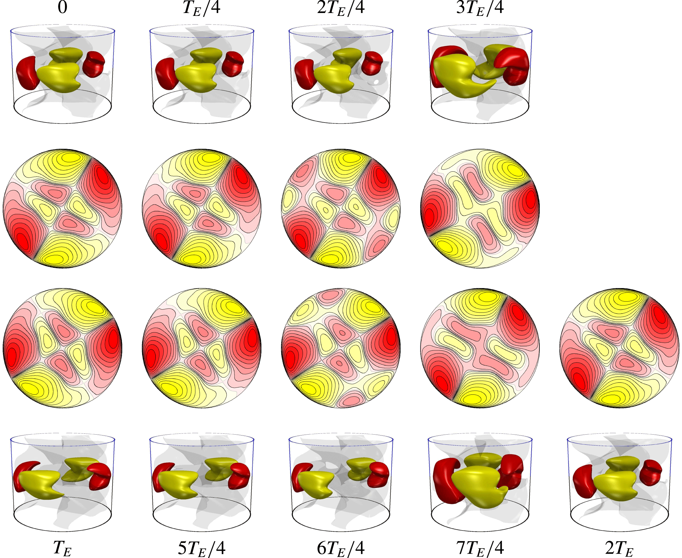
Snapshots of
 $w{-}w_{0}$
isosurfaces and
 $w$
contours at
 $z=0$
over
 $2T_{E}$
relative to an arbitrary reference time for PWo at
 $(\unicode[STIX]{x1D6E4},\mathit{Re})=(1.50,210)$
. See the online movie 6 for an animation of isosurfaces of
 $w{-}w_{0}$
.

Another different pulse wave, PWo, was found at
 $(\unicode[STIX]{x1D6E4},\mathit{Re})=(1.50,210)$
. It only has 2 plateaus of
 $E_{2}$
energy instead of the 8 plateaus of PWs and PWa. Figure 26 shows the
 $E_{2}$
time evolution with the
 $w$
evolution, showing that PWo is a periodic solution, with period
 $2T_{E}$
, but the modal energies are
 $T_{E}$
periodic. Figure 27 shows snapshots of
 $w$
at the mid-plane together with isosurfaces of
 $w{-}w_{0}$
. It pulses back and forth every
 $2T_{E}$
, periodically switching its orientation, much like the DRW do. However, the oscillation is not smooth, but pulse-like. PWo have broken
 ${\mathcal{R}}_{\unicode[STIX]{x1D6FC}}$
symmetry, for any angle
 $\unicode[STIX]{x1D6FC}$
except
 $\unicode[STIX]{x03C0}$
, so there is a group orbit of PWo obtained by applying
 ${\mathcal{R}}_{\unicode[STIX]{x1D6FC}}$
. Furthermore, since PWo have broken
 ${\mathcal{H}}_{\unicode[STIX]{x1D6FE}}$
symmetry, there are two group orbits, one obtained by applying
 ${\mathcal{H}}_{\unicode[STIX]{x1D6FE}}$
to the other (the angle
 $\unicode[STIX]{x1D6FE}$
is arbitrary, different values of
 $\unicode[STIX]{x1D6FE}$
will give a PWo on the other group orbit with a different orientation). PWo also have a space–time symmetry, a half-period-flip symmetry, where the flip is a composition of
 ${\mathcal{H}}_{\unicode[STIX]{x1D6FE}}$
with a rotation. This half-period-flip symmetry can be seen by comparing the solution at some time
 $t$
with the solution at
 $t+T_{E}$
, particularly in the contours of
 $w$
at the mid-plane as shown in figure 27.
In summary, the PWo has invariances
 ${\mathcal{R}}_{\unicode[STIX]{x03C0}}\boldsymbol{u}=\boldsymbol{u}$
,
 ${\mathcal{T}}_{2T_{E}}\boldsymbol{u}=\boldsymbol{u}$
, and
 ${\mathcal{T}}_{T_{E}}\boldsymbol{u}={\mathcal{R}}_{\unicode[STIX]{x1D719}-2\unicode[STIX]{x1D6FE}}{\mathcal{H}}_{\unicode[STIX]{x1D6FE}}\boldsymbol{u}$
for
 $\unicode[STIX]{x1D6FE}$
arbitrary and a given
 $\unicode[STIX]{x1D719}$
.
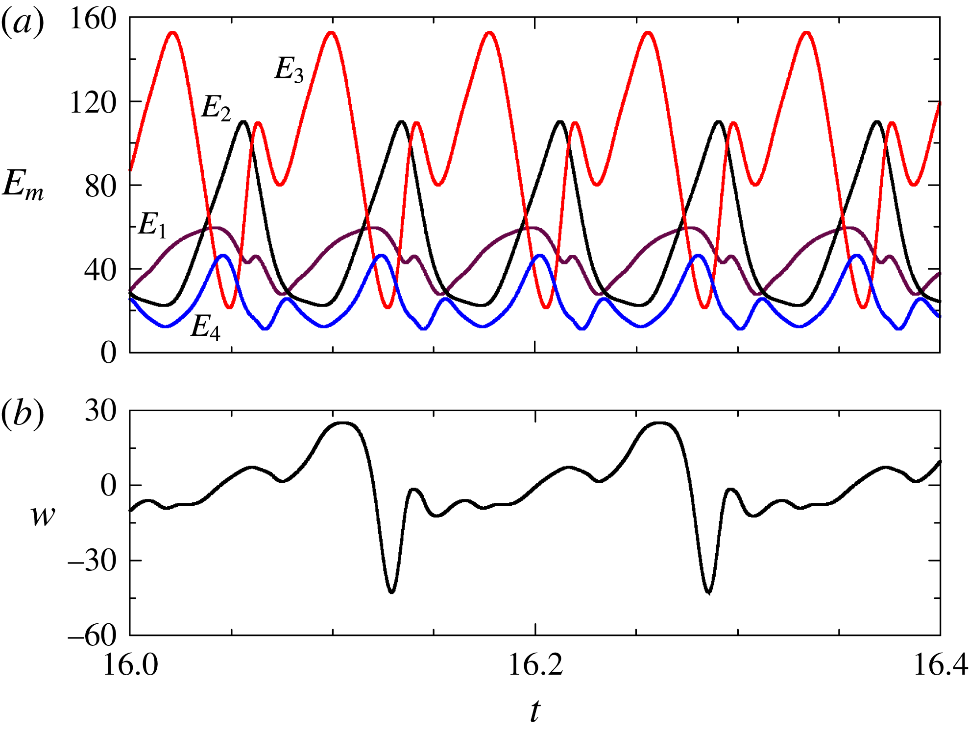
Time series of (a) modal kinetic energies
 $E_{1}$
,
 $E_{2}$
,
 $E_{3}$
and
 $E_{4}$
and (b)
 $w(0.98,0,-0.4\unicode[STIX]{x1D6E4})$
for LC at
 $(\unicode[STIX]{x1D6E4},\mathit{Re})=(1.9,275)$
.

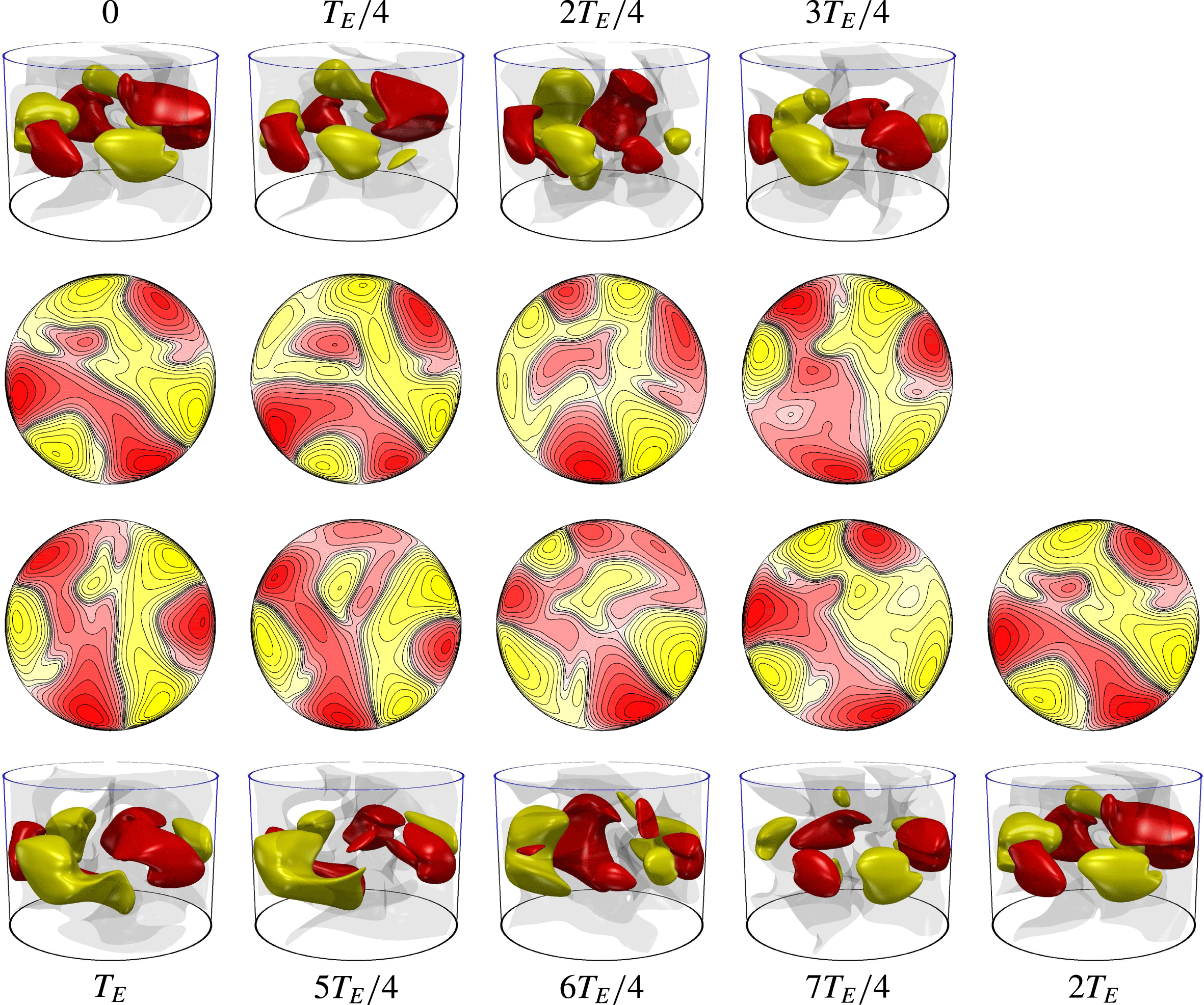
Snapshots of
 $w{-}w_{0}$
isosurfaces and
 $w$
contours at
 $z=0$
over
 $2T_{E}$
relative to an arbitrary reference time for LC at
 $(\unicode[STIX]{x1D6E4},\mathit{Re})=(1.90,275)$
. See the online movie 7 for an animation of isosurfaces of
 $w{-}w_{0}$
.

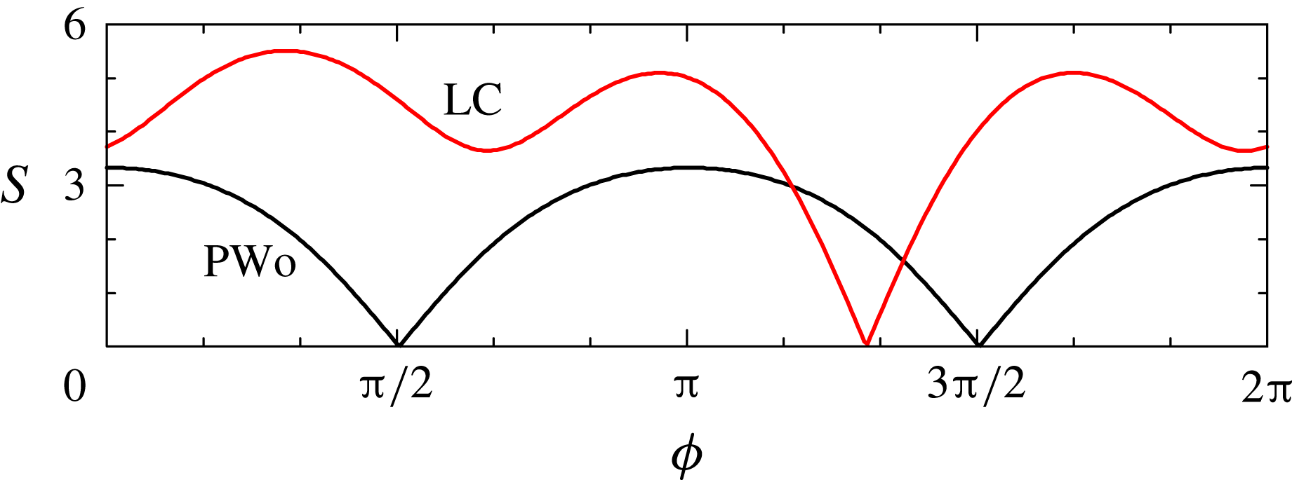
Variation of the symmetry measure
 $S$
, using
 ${\mathcal{H}}_{0}$
, with the rotation angle
 $\unicode[STIX]{x1D719}$
for PWo at
 $(\unicode[STIX]{x1D6E4},\mathit{Re})=(1.50,210)$
and LC at
 $(\unicode[STIX]{x1D6E4},\mathit{Re})=(1.90,275)$
.

In the upper ranges of parameter space investigated, with
 $\unicode[STIX]{x1D6E4}\sim 2$
and
 $\mathit{Re}\sim 300$
(indicated in the upper right corner of figure 23) we have encountered limit cycles, LC, which do not have any non-trivial spatial symmetry. Figure 28 shows the time evolution of the leading modal kinetic energies and
 $w(0.98,0,-0.4\unicode[STIX]{x1D6E4})$
for LC at
 $(\unicode[STIX]{x1D6E4},\mathit{Re})=(1.90,275)$
. Unlike the pulse wave states, LC does not exhibit slow–fast dynamics. The period in
 $w$
is
 $2T_{E}$
, twice the period in the modal energies. This suggests that like PWo, LC has a space–time symmetry. Figure 29 shows snap-shots of
 $w{-}w_{0}$
isosurfaces and of
 $w$
contours at
 $z=0$
, and together with the associated online movie 7, these allows us to determine the space–time symmetry of LC. Just like with PWo, applying
 ${\mathcal{H}}_{\unicode[STIX]{x1D6FE}}$
, for any
 $\unicode[STIX]{x1D6FE}$
, followed by the rotation
 ${\mathcal{R}}_{\unicode[STIX]{x1D719}-2\unicode[STIX]{x1D6FE}}$
for a specific
 $\unicode[STIX]{x1D719}$
, to LC at any time
 $t_{0}$
results in LC at
 $t_{0}+T_{E}$
. To better illustrate this space–time symmetry and to provide a way to determine
 $\unicode[STIX]{x1D719}$
for a given
 $\unicode[STIX]{x1D6FE}$
, we defined a symmetry measure
 $$\begin{eqnarray}S=\Vert {\mathcal{R}}_{\unicode[STIX]{x1D719}-2\unicode[STIX]{x1D6FE}}{\mathcal{H}}_{\unicode[STIX]{x1D6FE}}\boldsymbol{u}-{\mathcal{T}}_{T_{E}}\boldsymbol{u}\Vert _{2}.\end{eqnarray}$$
Without loss of generality, figure 30 shows the symmetry measure
 $S$
, calculated for a PWo state and a LC state when
 ${\mathcal{H}}_{0}$
is applied and considering
 $\unicode[STIX]{x1D719}\in [0,2\unicode[STIX]{x03C0}]$
. The symmetry measure is zero only for a specific
 $\unicode[STIX]{x1D719}=\unicode[STIX]{x1D719}_{0}$
(for PWo,
 $S=0$
also for
 $\unicode[STIX]{x1D719}=\unicode[STIX]{x1D719}_{0}\pm \unicode[STIX]{x03C0}$
because PWo is
 ${\mathcal{R}}_{\unicode[STIX]{x03C0}}$
symmetric). For any other
 $\unicode[STIX]{x1D6FE}$
,
 $S=0$
at
 $\unicode[STIX]{x1D719}=\unicode[STIX]{x1D719}_{0}-2\unicode[STIX]{x1D6FE}$
. Apart from not having slow–fast behaviour, the other main difference between LC and PWo is that while both have comparable levels of
 $E_{2}$
, for LC the level of
 $E_{3}$
is significantly larger than any other
 $E_{m}$
most of the time, and this leads to LC not having any non-trivial spatial symmetry.
In summary, LC has invariances
 ${\mathcal{T}}_{2T_{E}}\boldsymbol{u}=\boldsymbol{u}$
and
 ${\mathcal{T}}_{T_{E}}\boldsymbol{u}={\mathcal{R}}_{\unicode[STIX]{x1D719}-2\unicode[STIX]{x1D6FE}}{\mathcal{H}}_{\unicode[STIX]{x1D6FE}}\boldsymbol{u}$
for
 $\unicode[STIX]{x1D6FE}$
arbitrary and a given
 $\unicode[STIX]{x1D719}$
.
4 Discussion and conclusions
The dynamics of the flow in the split counter-rotating cylinder is dominated by the
 $O(2)$
symmetry of the system. The
 $O(2)$
symmetric basic state consists of two counter-rotating bodies of fluid, each completely contained within their respective half-cylinders, separated by a plane at the cylinder mid-height to which the vortex lines are tangential. The vortex lines being tangential to the mid-plane results in an azimuthal shear layer that also has a radial jet profile due to the vortex line bending. This basic state configuration becomes unstable with increasing counter rotation (quantified non-dimensionally by
 $\mathit{Re}$
); the critical
 $\mathit{Re}$
is smaller for larger cylinder aspect ratios
 $\unicode[STIX]{x1D6E4}$
. The primary instabilities are circle-pitchfork bifurcations, spawning group orbits of steady states
 $\text{S}m$
with azimuthal wavenumbers
 $m$
. The value of
 $m$
depends on
 $\unicode[STIX]{x1D6E4}$
, and for the range considered (
 $\unicode[STIX]{x1D6E4}\in [0.5,2.0]$
),
 $m$
ranges from 6 to 2. There are a number of codim-2 points where two curves of circle-pitchfork bifurcations cross in
 $(\unicode[STIX]{x1D6E4},\mathit{Re})$
parameter space, one curve corresponding to azimuthal wavenumber
 $m$
and the other to
 $m+1$
. We have studied in detail the dynamics in the neighbourhood of the 2 : 3 codim-2 point, and the resulting mode interactions are well described by the associated normal form.
Further away in parameter space from the primary circle-pitchfork bifurcations, we have found a number of other bifurcations and states. Some of these states are unstable due to broken symmetries, and by computing in the appropriate symmetric subspaces we have been able to study their dynamics. We have found rotating waves and direction reversing waves that result from either steady or Hopf bifurcations breaking the involution
 ${\mathcal{H}}$
symmetry of the
 $\text{S}m$
from which they bifurcate. These time-periodic states are typical of
 $O(2)$
symmetric systems. However, over much of the parameter space studied, these are not the predominant unsteady states found. Instead, we find that a variety of pulse wave states dominate the unsteady flow regimes. These are primarily characterized by slow–fast dynamics, with the slow phase corresponding to a particular orientation of a steady non-axisymmetric state, typically S2, and the fast phase corresponds to a rapid shift to a different orientation in the S2 group. Some pulse waves (PWs and PWo) reside in the symmetric subspace with only even Fourier azimuthal modes, while others (PWa) do not. We have also found other limit cycle solutions. All of these can be viewed as different choreographies as the vortex lines from one half of the cylinder try to penetrate into the other half, and the two sets of counter-rotating vortex lines negotiate their respective penetrations via flow configurations with different spatio-temporal symmetries.
All of the dynamics we have described is inherently related to how the
 $O(2)$
symmetry of the system is broken as
 $\mathit{Re}$
and
 $\unicode[STIX]{x1D6E4}$
are varied. The
 $O(2)$
symmetry owes its presence to the exact counter rotation of the two halves of the cylinder. Any slight difference in the rotation rates or the cylinder not being exactly split in half would result in the system only having
 $SO(2)$
symmetry. This then raises the question of how robust is the dynamics reported to slight imperfections. In the related von Kármán swirling flow, Nore et al. (Reference Nore, Moisy and Quartier2005) showed experimentally that much of the
 $O(2)$
-related dynamics persists in the face of experimental imperfections and noise. The details of the basic state and its bifurcations for the von Kármán swirling flow differ from those of the split-cylinder flow, primarily due to the viscous drag from the stationary sidewall leading to very different vortex line distributions in the basic state and consequently undergoing different bifurcations. Yet, there are many similarities between the two flows and this is due to both systems being
 $O(2)$
symmetric. In both cases the basic state first loses stability via circle-pitchfork bifurcations to three-dimensional steady states
 $\text{S}m$
, but the azimuthal wavenumber
 $m$
in the two cases differs. In both cases there are mode interactions where two circle-pitchfork bifurcations occur simultaneously, and these codim-2 points organize the dynamics over a sizable region of parameter space, displaying various rotating and pulse waves. Given the experimentally observed robustness of the
 $O(2)$
dynamics in the von Kármán swirling flow, it would be of interest to determine the effects of imperfections on the split-cylinder flow. In particular, the pulse waves can be viewed as a dynamic where the flow is a structure pinned to one particular orientation undergoing a very slow change until it de-pins and then quickly pins to another orientation. We found that the pulse waves PWa cease to exist via a SNIC bifurcation, whereby the structure remains pinned in a particular orientation indefinitely. Pinning and depinning of rotating waves in
 $SO(2)$
differentially rotating systems have also been reported and the role of imperfect symmetry has been investigated (Abshagen et al.
Reference Abshagen, Heise, Hoffmann and Pfister2008; Lopez & Marques Reference Lopez and Marques2009; Pacheco, Lopez & Marques Reference Pacheco, Lopez and Marques2011; Marques et al.
Reference Marques, Meseguer, Lopez, Pacheco and Lopez2013). These studies showed that SNIC bifurcations are predominant in the associated dynamics, but the details become extremely complicated. An investigation of imperfect
 $O(2)$
symmetry in the split-cylinder flow would be an interesting future exercise.
Acknowledgement
This work was supported by the US National Science Foundation grant CBET-1336410.
Supplementary movies
Supplementary movies are available at https://doi.org/10.1017/jfm.2017.103.