1 Introduction
The latest advancements in wavelet-based numerical methodologies to solve partial differential equations (Vasilyev, Yuen & Paolucci Reference Vasilyev, Yuen and Paolucci1997; Vasilyev Reference Vasilyev2003; Vasilyev & Kevlahan Reference Vasilyev and Kevlahan2005; Nejadmalayeri et al. Reference Nejadmalayeri, Vezolainen, Brown-Dymkoski and Vasilyev2015; Souopgui et al. Reference Souopgui, Wieland, Hussaini and Vasilyev2016), combined with the unique properties of wavelet analysis to identify and isolate localized dynamically dominant flow structures (Farge et al. Reference Farge, Schneider, Pellegrino, Wray and Rogallo2003; Goldstein & Vasilyev Reference Goldstein and Vasilyev2004), and to track them on adaptive computational meshes (Vasilyev & Kevlahan Reference Vasilyev and Kevlahan2002; Goldstein, Vasilyev & Kevlahan Reference Goldstein, Vasilyev and Kevlahan2005; Kevlahan & Vasilyev Reference Kevlahan and Vasilyev2005), have demonstrated the benefits of using spatio-temporal mesh adaptation for numerical simulations of turbulent flows. The wavelet-based methods with inherent adaptive mesh refinement capabilities and sparse data representation not only take full advantage of spatio-temporal intermittency of turbulent flows by substantially reducing the number of degrees of freedom and, consequently, the computational cost, but also provide a systematic framework for active error control.
Further tight integration of an adaptive wavelet-based method with turbulence modelling allows a construction of a hierarchical framework for simulating turbulent flows (De Stefano & Vasilyev Reference De Stefano and Vasilyev2012) where coherent flow structures are either totally or partially resolved on self-adaptive computational grids, while modelling the effect of unresolved motions. The separation between resolved (more energetic) eddies and residual (less energetic) flow structures is achieved by means of the nonlinear wavelet thresholding filter. The value of wavelet threshold controls the relative importance of resolved field and residual background flow and, thus, the fidelity of turbulence simulations. By increasing the thresholding level a unified hierarchy of wavelet-based turbulence models of different fidelity can be obtained. Wavelet-based direct numerical simulation (W-DNS), coherent vortex simulation (CVS) (Farge et al. Reference Farge, Schneider, Pellegrino, Wray and Rogallo2003) and wavelet-based stochastic coherent adaptive large-eddy simulation (SCALES) (Goldstein & Vasilyev Reference Goldstein and Vasilyev2004; De Stefano & Vasilyev Reference De Stefano and Vasilyev2010), also referred to as adaptive LES (De Stefano & Vasilyev Reference De Stefano and Vasilyev2013), represent different fidelity methods within this hierarchy. A distinct advantage of the adaptive wavelet-based hierarchical framework is that the overall physical fidelity of the simulation can be simply controlled by the adaptive wavelet threshold filter (Nejadmalayeri et al. Reference Nejadmalayeri, Vezolainen, De Stefano and Vasilyev2014; De Stefano, Nejadmalayeri & Vasilyev Reference De Stefano, Nejadmalayeri and Vasilyev2016), thereby providing a fully unified hierarchical modelling framework that allows transition continuously among various fidelities, from W-DNS to CVS to adaptive LES, and even to wavelet-based adaptive unsteady Reynolds-averaged Navier–Stokes (W-URANS) simulations (De Stefano, Vasilyev & Brown-Dymkoski Reference De Stefano, Vasilyev and Brown-Dymkoski2018; Ge et al. Reference Ge, Vasilyev, De Stefano and Hussaini2018).
Transition from DNS to CVS to adaptive LES is well established through controlling the wavelet threshold. W-DNS uses wavelet-based discretization of the Navier–Stokes equations to adapt dynamically the local resolution of intermittent flow structures (Vasilyev & Kevlahan Reference Vasilyev and Kevlahan2002; Brown-Dymkoski, Kasimov & Vasilyev Reference Brown-Dymkoski, Kasimov and Vasilyev2014; De Stefano & Vasilyev Reference De Stefano and Vasilyev2014). Transition from W-DNS to CVS (Farge et al. Reference Farge, Schneider, Pellegrino, Wray and Rogallo2003) is achieved by using an optimal wavelet threshold, resulting in the decomposition of the flow field into coherent and incoherent contributions. For adaptive LES, the wavelet threshold is further increased so that the stochastic and the least energetic coherent portion of the turbulent solution are discarded and only the most energetic part of the coherent vortices are captured in the resolved field (Goldstein & Vasilyev Reference Goldstein and Vasilyev2004). In adaptive LES, the discarded sub-grid-scale (SGS) coherent structures dominate the total SGS dissipation (Goldstein & Vasilyev Reference Goldstein and Vasilyev2004; De Stefano, Goldstein & Vasilyev Reference De Stefano, Goldstein and Vasilyev2005). Therefore, similar to conventional LES methods, many standard LES closures are applicable to the adaptive LES method by modelling SGS coherent structures in terms of the resolved energetic coherent vortices (De Stefano, Vasilyev & Goldstein Reference De Stefano, Vasilyev and Goldstein2008; Vasilyev et al. Reference Vasilyev, De Stefano, Goldstein and Kevlahan2008).
The transition to the W-URANS regime is not as straightforward. In the RANS equations, the unknown variables are mean (Reynolds-averaged or Favre-averaged) quantities, which are smooth and whose evolution is described by dissipative models. As shown in De Stefano et al. (Reference De Stefano, Vasilyev and Brown-Dymkoski2018), the accurate solution of RANS equations, even on adaptive meshes as in W-URANS, requires the use of low wavelet threshold values compared to the ones used in W-DNS, which is counter-intuitive when compared to the monotonically increasing threshold value for decreasing fidelity from the W-DNS to CVS to adaptive LES regimes. The objective of the present study is to develop a hybrid mathematically consistent approach with coexistence, connection and even active communication between the W-URANS and adaptive LES regions. The current work serves as a crucial step towards construction of a unified wavelet-based adaptive hierarchical RANS/LES modelling framework, capable of performing simulations of various fidelity from no-modelling direct numerical simulations to full-modelling RANS simulations.
It is important to emphasize that in contrast to conventional hybrid RANS/LES methods where the grid is specified a priori, our approach uses a dynamically adaptive grid. A variable wavelet thresholding strategy blending two distinct thresholds for the W-URANS and adaptive LES regimes is used. In addition, a novel mesh adaptation on mean and fluctuating quantities with different wavelet thresholds levels is proposed. The effectiveness of the wavelet-based adaptive delayed detached eddy simulation (W-DDES) method is demonstrated by comparing the results of the W-DDES simulations with the results already available in the literature. Supersonic plane channel flows for two different configurations, a subsonic channel flow with periodic hill constrictions and a supersonic flow over a compression ramp are investigated as benchmark wall-bounded problems for compressible flows.
This paper is organized as follows. Section 2 introduces the governing equations of the simulations, including the Favre-filtered Navier–Stokes equations for compressible flows and the evolution equations for the turbulence model. The primary wavelet-based adaptive methods and the adaptive-anisotropic wavelet collocation method (A-AWCM) for complex domain geometries are described in § 3. Section 4 describes the novel adaptation strategy treating different flow regimes and mean and fluctuating quantities elaborately. The simulations and corresponding results are presented and discussed in § 5. Concluding remarks are given at the end in § 6.
2 Governing equations
2.1 Favre-filtered Navier–Stokes equations
The W-DDES approach integrates W-URANS and adaptive LES approaches, described by different equations. For compressible flows W-URANS is formulated in terms of Reynolds-averaged (i.e. density and pressure) and Favre-averaged (i.e. velocity and temperature) dependent variables, whereas the adaptive LES are formulated in terms of wavelet- and wavelet-Favre-filtered dependent variables. At first glance it is inconsistent to have both time-filtered (RANS) and spatially (wavelet) filtered (LES) quantities simultaneously in a hybrid modelling method. However, the family of eddy-resolving detached eddy simulation (DES) models is better described in terms of length scale formulation (Durbin Reference Durbin2018) that adopts either RANS equations in the near-wall region or a low-pass (wavelet) filtered Naiver–Stokes equations in LES region away from the wall. The DES approach is essentially an eddy-resolving method everywhere as it has to be ensemble averaged to obtain statistical quantities. Significant levels of fluctuations are usually observed, even in the so-called RANS regions of the domain. Therefore, the term ‘Favre filtered’ is used for all dependent variables in the W-DDES formulation.
For conventional non-adaptive LES, the implicit or explicit linear lowpass-filtering operator is usually defined a priori and is tight to the corresponding computational mesh with under-resolved grid spacings relative to DNS. In contrast to standard LES, the wavelet-filtering operator used in the adaptive LES is constructed by using the wavelet thresholding described in § 3.1, which is nonlinear and depends on the instantaneous flow realization. One can define a wavelet-filtering operator for a variable
 $\unicode[STIX]{x1D719}$
as
 $\overline{\unicode[STIX]{x1D719}}^{{>}\unicode[STIX]{x1D716}}$
. The conventional lowpass-Favre filter for variable density flows can be denoted as
 $\widehat{\unicode[STIX]{x1D719}}=\overline{\unicode[STIX]{x1D70C}\unicode[STIX]{x1D719}}/\overline{\unicode[STIX]{x1D70C}}$
, where the overbar
 $\overline{(\cdot )}$
represents the lowpass filter. Therefore, the wavelet-Favre filter can be written as
 $\widehat{\unicode[STIX]{x1D719}}^{{>}\unicode[STIX]{x1D716}}=\overline{\unicode[STIX]{x1D70C}\unicode[STIX]{x1D719}}^{{>}\unicode[STIX]{x1D716}}/\overline{\unicode[STIX]{x1D70C}}^{{>}\unicode[STIX]{x1D716}}$
. Consequently in the wavelet-Favre-filtered Navier–Stokes equations, the primitive variables are
 $\overline{\unicode[STIX]{x1D70C}}^{{>}\unicode[STIX]{x1D716}}$
,
 $\overline{p}^{{>}\unicode[STIX]{x1D716}}$
,
 $\widehat{u_{i}}^{{>}\unicode[STIX]{x1D716}}$
,
 $\widehat{T}^{{>}\unicode[STIX]{x1D716}}$
and
 $\widehat{e}^{{>}\unicode[STIX]{x1D716}}$
representing respectively the wavelet-filtered density of the fluid (gas) and pressure and the wavelet-Favre-filtered velocity, temperature and total energy per unit mass. For the sake of simplicity, the variables
 $\unicode[STIX]{x1D70C}$
,
 $p$
,
 $u_{i}$
,
 $T$
and
 $e$
are used hereafter to represent all the primitive variables. Subsequently, the wavelet-Favre-filtered Navier–Stokes equations for conservation of mass, momentum and energy in compressible flows of calorically perfect gas with modelled turbulent terms can be written in the following form:
 $$\begin{eqnarray}\displaystyle & \displaystyle \frac{\unicode[STIX]{x2202}\unicode[STIX]{x1D70C}}{\unicode[STIX]{x2202}t}+\frac{\unicode[STIX]{x2202}(\unicode[STIX]{x1D70C}u_{j})}{\unicode[STIX]{x2202}x_{j}}=0, & \displaystyle\end{eqnarray}$$
 $$\begin{eqnarray}\displaystyle & \displaystyle \frac{\unicode[STIX]{x2202}\unicode[STIX]{x1D70C}u_{i}}{\unicode[STIX]{x2202}t}+\frac{\unicode[STIX]{x2202}}{\unicode[STIX]{x2202}x_{j}}(\unicode[STIX]{x1D70C}u_{i}u_{j})=-\frac{\unicode[STIX]{x2202}p}{\unicode[STIX]{x2202}x_{i}}+\frac{\unicode[STIX]{x2202}\hat{\unicode[STIX]{x1D70F}}_{ij}}{\unicode[STIX]{x2202}x_{j}}, & \displaystyle\end{eqnarray}$$
 $$\begin{eqnarray}\displaystyle & \displaystyle \frac{\unicode[STIX]{x2202}\unicode[STIX]{x1D70C}e}{\unicode[STIX]{x2202}t}+\frac{\unicode[STIX]{x2202}}{\unicode[STIX]{x2202}x_{j}}[(\unicode[STIX]{x1D70C}e+p)u_{j}]=\frac{\unicode[STIX]{x2202}}{\unicode[STIX]{x2202}x_{j}}[u_{i}\hat{\unicode[STIX]{x1D70F}}_{ij}-q_{j}], & \displaystyle\end{eqnarray}$$
where
 $$\begin{eqnarray}\displaystyle & \displaystyle p=\unicode[STIX]{x1D70C}RT, & \displaystyle\end{eqnarray}$$
 $$\begin{eqnarray}\displaystyle & \displaystyle e=\frac{1}{2}u_{i}u_{i}+\frac{p}{\unicode[STIX]{x1D70C}(\unicode[STIX]{x1D6FE}-1)}, & \displaystyle\end{eqnarray}$$
 $$\begin{eqnarray}\displaystyle & \displaystyle q_{j}=-c_{p}\left(\frac{\unicode[STIX]{x1D707}}{Pr_{L}}+\frac{\unicode[STIX]{x1D707}_{T}}{Pr_{T}}\right)\frac{\unicode[STIX]{x2202}T}{\unicode[STIX]{x2202}x_{j}}, & \displaystyle\end{eqnarray}$$
 $$\begin{eqnarray}\left.\begin{array}{@{}c@{}}\displaystyle \hat{\unicode[STIX]{x1D70F}}_{ij}=2\unicode[STIX]{x1D707}\tilde{\unicode[STIX]{x1D61A}}_{ij}+\unicode[STIX]{x1D70F}_{ij},\\ \displaystyle \unicode[STIX]{x1D70F}_{ij}=2\unicode[STIX]{x1D707}_{T}\tilde{\unicode[STIX]{x1D61A}}_{ij},\\ \displaystyle \tilde{\unicode[STIX]{x1D61A}}_{ij}=\text{dev}(\unicode[STIX]{x1D61A}_{ij})=\unicode[STIX]{x1D61A}_{ij}-\frac{1}{3}\frac{\unicode[STIX]{x2202}u_{k}}{\unicode[STIX]{x2202}x_{k}}\unicode[STIX]{x1D6FF}_{ij},\\ \displaystyle \unicode[STIX]{x1D61A}_{ij}=\frac{1}{2}\left(\frac{\unicode[STIX]{x2202}u_{i}}{\unicode[STIX]{x2202}x_{j}}+\frac{\unicode[STIX]{x2202}u_{j}}{\unicode[STIX]{x2202}x_{i}}\right).\end{array}\right\}\end{eqnarray}$$
Parameter
 $R$
is the gas constant, while
 $c_{v}$
and
 $c_{p}$
are the specific heat constants at constant volume and pressure, respectively. The specific heat ratio
 $\unicode[STIX]{x1D6FE}=c_{p}/c_{v}\equiv 1.4$
for diatomic gases, and
 $Pr=(\unicode[STIX]{x1D707}c_{p})/\unicode[STIX]{x1D706}$
is the Prandtl number. The term
 $q_{j}$
is the sum of both the laminar and modelled turbulent heat fluxes with
 $Pr_{L}=0.72$
and
 $Pr_{T}=0.9$
being the laminar and turbulent Prandtl numbers respectively. The turbulent eddy viscosity is denoted by
 $\unicode[STIX]{x1D707}_{T}$
, which is unknown and needs turbulence models for closure. The term
 $\hat{\unicode[STIX]{x1D70F}}_{ij}$
is the sum of the molecular and Reynolds stress tensors, while
 $\unicode[STIX]{x1D70F}_{ij}$
is the Reynolds stress tensor,
 $\unicode[STIX]{x1D61A}_{ij}$
is the mean strain-rate tensor and
 $\tilde{\unicode[STIX]{x1D61A}}_{ij}$
is the deviatoric tensor of
 $\unicode[STIX]{x1D61A}_{ij}$
. The temperature-dependent dynamic molecular viscosity
 $\unicode[STIX]{x1D707}$
is given by Sutherland’s law,
 $$\begin{eqnarray}{\displaystyle \frac{\unicode[STIX]{x1D707}}{\unicode[STIX]{x1D707}_{ref}}}={\displaystyle \frac{T_{ref}+S}{T+S}}\left({\displaystyle \frac{T}{T_{ref}}}\right)^{3/2},\end{eqnarray}$$
where the constants
 $S=110.4K$
and
 $T_{ref}=293.15K$
.
2.2 Turbulence model equations
The delayed detached eddy simulation (DDES) model employed in this work is the Spalart–Allmaras (S–A) model based DDES (Spalart et al.
Reference Spalart, Deck, Shur, Squires, Strelets and Travin2006). This model is an improved version of the original DES model (Spalart et al.
Reference Spalart, Jou, Strelets and Allmaras1997) with a crucial re-defining of the DES length scale
 $\tilde{d}$
in terms of a shielding function
 $f_{d}$
, which is written as
 $$\begin{eqnarray}f_{d}\equiv 1-\tanh ([8r_{d}]^{3}),\end{eqnarray}$$
with its argument
 $r_{d}$
given by
 $$\begin{eqnarray}r_{d}\equiv {\displaystyle \frac{\unicode[STIX]{x1D708}_{T}+\unicode[STIX]{x1D708}}{\sqrt{u_{i,j}u_{i,j}}\unicode[STIX]{x1D705}^{2}d^{2}}},\end{eqnarray}$$
where
 $\unicode[STIX]{x1D708}_{T}$
is the kinematic eddy viscosity,
 $\unicode[STIX]{x1D708}$
is the molecular viscosity,
 $u_{i,j}$
is the velocity gradient tensor,
 $\unicode[STIX]{x1D705}$
is the Kármán constant and
 $d$
is the distance to the wall. The parameter
 $r_{d}$
is unity in the log layer, and gradually falls to 0 at the edge of the boundary layer. Therefore,
 $f_{d}$
vanishes within the log layer and increases to 1 out of the boundary layer. The length scale
 $\tilde{d}$
replaces the wall distance
 $d$
, namely the RANS length scale in the S–A model, and
 $\tilde{d}$
has the following form:
 $$\begin{eqnarray}\tilde{d}\equiv l_{RANS}-f_{d}\max (0,l_{RANS}-l_{LES}),\end{eqnarray}$$
where
 $l_{RANS}=d$
,
 $l_{LES}=\unicode[STIX]{x1D6F9}C_{DES}\unicode[STIX]{x1D6E5}$
and
 $\unicode[STIX]{x1D6E5}$
is the sub-grid length scale given by maximum local grid spacing among three Cartesian directions in the physical domain, namely
 $$\begin{eqnarray}\unicode[STIX]{x1D6E5}=\max (\unicode[STIX]{x1D6E5}_{x},\unicode[STIX]{x1D6E5}_{y},\unicode[STIX]{x1D6E5}_{z}),\end{eqnarray}$$
 $C_{DES}=0.65$
is an empirical constant (Shur et al.
Reference Shur, Spalart, Strelets and Travin1999),
 $\unicode[STIX]{x1D6F9}$
is a low Reynolds number correction (Spalart et al.
Reference Spalart, Deck, Shur, Squires, Strelets and Travin2006) given by
 $$\begin{eqnarray}\unicode[STIX]{x1D6F9}^{2}=\min \left[10^{2},{\displaystyle \frac{1-\displaystyle {\displaystyle \frac{c_{b1}}{c_{w1}\unicode[STIX]{x1D705}^{2}f_{w}^{\ast }}}[f_{t2}+(1-f_{t2})f_{v2}]}{f_{v1}\max (10^{-10},1-f_{t2})}}\right],\end{eqnarray}$$
 $f_{w}^{\ast }=0.424$
and other constant coefficients follow the original S–A model and are described below. Note that in RANS mode
 $f_{d}=0$
,
 $\tilde{d}=d$
, whereas in LES mode
 $f_{d}=1$
and, thus,
 $\tilde{d}=\min (d,\unicode[STIX]{x1D6F9}C_{DES}\unicode[STIX]{x1D6E5})$
. Using the blending or shielding function
 $f_{d}$
, the RANS mode is shielded or delayed, up to the log layer, whereas for the original DES model, the LES mode may take over the RANS mode earlier below the log layer at intermediate cell aspect ratios, which causes the modelled-stress depletion (MSD) (Spalart et al.
Reference Spalart, Deck, Shur, Squires, Strelets and Travin2006).
The standard Spalart–Allmaras model (Spalart & Allmaras Reference Spalart and Allmaras1992) in terms of
 $\unicode[STIX]{x1D70C}\tilde{\unicode[STIX]{x1D708}}$
is written as
 $$\begin{eqnarray}\displaystyle & & \displaystyle \frac{\unicode[STIX]{x2202}\unicode[STIX]{x1D70C}\tilde{\unicode[STIX]{x1D708}}}{\unicode[STIX]{x2202}t}+\frac{\unicode[STIX]{x2202}}{\unicode[STIX]{x2202}x_{j}}(\unicode[STIX]{x1D70C}\tilde{\unicode[STIX]{x1D708}}u_{j})=c_{b1}(1-f_{t2})\tilde{S}\unicode[STIX]{x1D70C}\tilde{\unicode[STIX]{x1D708}}-\left[c_{w1}f_{w}-\frac{c_{b1}}{\unicode[STIX]{x1D705}^{2}}f_{t2}\right]\unicode[STIX]{x1D70C}\left(\frac{\tilde{\unicode[STIX]{x1D708}}}{\tilde{d}}\right)^{2}\nonumber\\ \displaystyle & & \displaystyle \quad +\,\frac{\unicode[STIX]{x2202}}{\unicode[STIX]{x2202}x_{j}}\left[\left(\frac{\unicode[STIX]{x1D707}}{\unicode[STIX]{x1D70E}}+\frac{\unicode[STIX]{x1D70C}\tilde{\unicode[STIX]{x1D708}}}{\unicode[STIX]{x1D70E}}\right)\frac{\unicode[STIX]{x2202}\tilde{\unicode[STIX]{x1D708}}}{\unicode[STIX]{x2202}x_{j}}\right]-\left(\frac{\unicode[STIX]{x1D707}}{\unicode[STIX]{x1D70E}\unicode[STIX]{x1D70C}}+\frac{\tilde{\unicode[STIX]{x1D708}}}{\unicode[STIX]{x1D70E}}\right)\frac{\unicode[STIX]{x2202}\unicode[STIX]{x1D70C}}{\unicode[STIX]{x2202}x_{j}}\frac{\unicode[STIX]{x2202}\tilde{\unicode[STIX]{x1D708}}}{\unicode[STIX]{x2202}x_{j}}+c_{b2}\frac{\unicode[STIX]{x1D70C}}{\unicode[STIX]{x1D70E}}\frac{\unicode[STIX]{x2202}\tilde{\unicode[STIX]{x1D708}}}{\unicode[STIX]{x2202}x_{j}}\frac{\unicode[STIX]{x2202}\tilde{\unicode[STIX]{x1D708}}}{\unicode[STIX]{x2202}x_{j}},\end{eqnarray}$$
and the eddy viscosity is computed from,
 $$\begin{eqnarray}\unicode[STIX]{x1D707}_{T}=\unicode[STIX]{x1D70C}\tilde{\unicode[STIX]{x1D708}}f_{v1}\end{eqnarray}$$
where
 $$\begin{eqnarray}\left.\begin{array}{@{}c@{}}\displaystyle f_{v1}={\displaystyle \frac{\unicode[STIX]{x1D712}^{3}}{\unicode[STIX]{x1D712}^{3}+c_{v1}^{3}}},\\ \displaystyle \unicode[STIX]{x1D712}=\tilde{\unicode[STIX]{x1D708}}/\unicode[STIX]{x1D708},\\ \displaystyle \tilde{S}=\max \left[0.3\sqrt{2\unicode[STIX]{x1D6FA}_{ij}\unicode[STIX]{x1D6FA}_{ij}},\sqrt{2\unicode[STIX]{x1D6FA}_{ij}\unicode[STIX]{x1D6FA}_{ij}}+\frac{\tilde{\unicode[STIX]{x1D708}}}{\unicode[STIX]{x1D705}^{2}\tilde{d}^{2}}f_{v2}\right],\\ \displaystyle \unicode[STIX]{x1D6FA}_{ij}=\frac{1}{2}\left(\frac{\unicode[STIX]{x2202}u_{i}}{\unicode[STIX]{x2202}x_{j}}-\frac{\unicode[STIX]{x2202}u_{j}}{\unicode[STIX]{x2202}x_{i}}\right),\\ \displaystyle f_{v2}=1-{\displaystyle \frac{\unicode[STIX]{x1D712}}{1+\unicode[STIX]{x1D712}f_{v1}}},\\ \displaystyle f_{w}=g\left[{\displaystyle \frac{1+c_{w3}^{6}}{g^{6}+c_{w3}^{6}}}\right]^{1/6},\\ \displaystyle g=r+c_{w2}(r^{6}-r),\\ \displaystyle r=\min \left[{\displaystyle \frac{\tilde{\unicode[STIX]{x1D708}}}{\tilde{S}\unicode[STIX]{x1D705}^{2}\tilde{d}^{2}}},10\right],\\ \displaystyle f_{t2}=c_{t3}\exp (-c_{t4}\unicode[STIX]{x1D712}^{2}),\end{array}\right\}\end{eqnarray}$$
and
 $\tilde{d}$
is the hybrid DDES length scale defined in (2.11). To avoid possible numerical problems, Spalart (private communication) suggests limiting
 $\tilde{S}$
to be no smaller than
 $0.3\sqrt{2\unicode[STIX]{x1D6FA}_{ij}\unicode[STIX]{x1D6FA}_{ij}}$
;
 $c_{b1}=0.1355$
,
 $c_{b2}=0.622$
,
 $\unicode[STIX]{x1D70E}=2/3$
,
 $\unicode[STIX]{x1D705}=0.41$
,
 $c_{w2}=0.3$
,
 $c_{w3}=2$
,
 $c_{v1}=7.1$
,
 $c_{w1}=c_{b1}/\unicode[STIX]{x1D705}+(1+c_{b2})/\unicode[STIX]{x1D70E}$
. This ‘standard’ version of the S–A model does not have the trip term ‘
 $f_{t1}$
’, and hence it is argued that
 $f_{t2}$
is not necessary, i.e.
 $c_{t3}=0$
. The no-slip wall boundary condition for
 $\tilde{\unicode[STIX]{x1D708}}$
is
 $\tilde{\unicode[STIX]{x1D708}}=0$
.
3 Wavelet-based adaptive computations
The turbulence models described above are implemented using the parallel adaptive wavelet collocation method (PAWCM) (Nejadmalayeri et al. Reference Nejadmalayeri, Vezolainen, Brown-Dymkoski and Vasilyev2015). The governing equations are evaluated at collocation points, which are adapted in space and time to dynamically resolve all the features of the numerical solution. The essential features of the PAWCM are briefly described below. For detailed discussion the reader is referred to Vasilyev & Bowman (Reference Vasilyev and Bowman2000), Vasilyev (Reference Vasilyev2003), Nejadmalayeri et al. (Reference Nejadmalayeri, Vezolainen, Brown-Dymkoski and Vasilyev2015) and Brown-Dymkoski & Vasilyev (Reference Brown-Dymkoski and Vasilyev2017). A novel treatment of periodic boundary conditions for anisotropic meshes is described in § 3.3.
3.1 Adaptive wavelet collocation method
The adaptive wavelet collocation method is based on multi-resolution wavelet analysis to construct time-dependent computational meshes with spatially varying resolution, required to adequately resolve the localized features of the solution with a priori prescribed accuracy. The grid adaptation is based on the analysis of wavelet decomposition of a spatially dependent field, say
 $u(\boldsymbol{x})$
, sampled on a set of dyadic nested collocation points
 $\boldsymbol{x}_{\boldsymbol{k}}^{j}$
at different levels of resolution
 $j$
, formally written as
 $$\begin{eqnarray}u(\boldsymbol{x})=\mathop{\sum }_{\boldsymbol{l}\in {\mathcal{L}}^{1}}c_{\boldsymbol{l}}^{1}\unicode[STIX]{x1D719}_{\boldsymbol{l}}^{1}(\boldsymbol{x})+\mathop{\sum }_{j=2}^{J}\mathop{\sum }_{\unicode[STIX]{x1D707}=1}^{2^{n}-1}\mathop{\sum }_{\boldsymbol{k}\in {\mathcal{K}}^{\unicode[STIX]{x1D707},j}}d_{\boldsymbol{k}}^{\unicode[STIX]{x1D707},j}\unicode[STIX]{x1D713}_{\boldsymbol{k}}^{\unicode[STIX]{x1D707},j}(\boldsymbol{x}),\end{eqnarray}$$
where
 $n$
denotes the number of spatial dimensions, bold subscripts denote
 $n$
-dimensional indices, while
 ${\mathcal{L}}^{1}$
and
 ${\mathcal{K}}^{\unicode[STIX]{x1D707},j}$
are
 $n$
-dimensional index sets associated with scaling functions
 $\unicode[STIX]{x1D719}_{\boldsymbol{l}}^{1}$
and wavelets
 $\unicode[STIX]{x1D713}_{\boldsymbol{k}}^{\unicode[STIX]{x1D707},j}$
, respectively. Each of the basis functions, i.e.
 $\unicode[STIX]{x1D719}_{\boldsymbol{l}}^{1}$
or
 $\unicode[STIX]{x1D713}_{\boldsymbol{k}}^{\unicode[STIX]{x1D707},j}$
, corresponds one-to-one with a grid point
 $\boldsymbol{l}\in {\mathcal{L}}^{1}$
or
 $\boldsymbol{k}\in {\mathcal{K}}^{\unicode[STIX]{x1D707},j}$
. Scaling functions
 $\unicode[STIX]{x1D719}_{\boldsymbol{l}}^{1}$
carry the averaged signal, while the multi-dimensional second-generation wavelet functions
 $\unicode[STIX]{x1D713}_{\boldsymbol{k}}^{\unicode[STIX]{x1D707},j}$
define local, variational details. The amplitudes are given by the coefficients
 $c_{\boldsymbol{l}}^{1}$
and
 $d_{\boldsymbol{k}}^{\unicode[STIX]{x1D707},j}$
, respectively, and hence have a unique correspondence to grid points. The levels of resolution span over
 $1\leqslant j\leqslant J$
, with
 $1$
and
 $J$
being respectively the coarsest and finest levels of resolution present in the approximation. During the wavelet transform, detail (or wavelet) coefficients
 $d_{\boldsymbol{k}}^{\unicode[STIX]{x1D707},j}$
are obtained recursively from scaling coefficients
 $c_{\boldsymbol{k}}^{\unicode[STIX]{x1D707},j}$
from level
 $J$
to 2. After wavelet transform, grid points
 $\boldsymbol{l}\in {\mathcal{L}}^{1}$
at the coarsest level store the scaling coefficients
 $c_{\boldsymbol{l}}^{1}$
, and all the other grid points
 $\boldsymbol{k}\in {\mathcal{K}}^{\unicode[STIX]{x1D707},j}$
at higher levels store the wavelet coefficients
 $d_{\boldsymbol{k}}^{\unicode[STIX]{x1D707},j}$
. To avoid ambiguity, grid points
 $\boldsymbol{k}\in {\mathcal{K}}^{\unicode[STIX]{x1D707},j}$
with
 $2\leqslant j\leqslant J$
represent all collocation points located at level
 $2\leqslant j\leqslant J$
. Note that for
 $n$
-dimensional space, there are
 $2^{n}-1$
families of wavelet functions, indexed by
 $\unicode[STIX]{x1D707}$
.
Wavelet threshold-filtering arises naturally from the series expansion (3.1). The filtering operation is performed by applying the wavelet transform to the original field
 $u(\boldsymbol{x})$
, zeroing the wavelet coefficients below a given threshold,
 $\unicode[STIX]{x1D716}=\unicode[STIX]{x1D716}(\boldsymbol{x},t)$
for generality, and transforming back to the physical space. The resulting approximate field, say
 $u^{{>}\unicode[STIX]{x1D716}}(\boldsymbol{x})$
, composed of a subset of the original wavelets, represents the dominant modes and can be formally written as the following conditional series:
 $$\begin{eqnarray}u^{{>}\unicode[STIX]{x1D716}}(\boldsymbol{x})=\mathop{\sum }_{\boldsymbol{l}\in {\mathcal{L}}^{1}}c_{\boldsymbol{l}}^{1}\unicode[STIX]{x1D719}_{\boldsymbol{l}}^{1}(\boldsymbol{x})+\mathop{\sum }_{j=2}^{J}\mathop{\sum }_{\unicode[STIX]{x1D707}=1}^{2^{n}-1}\mathop{\sum }_{\substack{ \boldsymbol{k}\in {\mathcal{K}}^{\unicode[STIX]{x1D707},j} \\ |d_{\boldsymbol{k}}^{\unicode[STIX]{x1D707},j}|>\unicode[STIX]{x1D716}\Vert u(\boldsymbol{x})\Vert }}d_{\boldsymbol{k}}^{\unicode[STIX]{x1D707},j}\unicode[STIX]{x1D713}_{\boldsymbol{k}}^{\unicode[STIX]{x1D707},j}(\boldsymbol{x}).\end{eqnarray}$$
In many implementations, the filter threshold is taken to be relative to some characteristic scale, often represented by either the
 $L_{2}$
or
 $L_{\infty }$
norm of
 $u(\boldsymbol{x})$
taken globally over the domain and denoted as
 $\Vert u(\boldsymbol{x})\Vert$
(Goldstein & Vasilyev Reference Goldstein and Vasilyev2004). The resulting nonlinear filtering operation practically separates resolved flow structures and unresolved residual motions. For a properly normalized threshold, the reconstruction error of the filtered variable is shown by Donoho (Reference Donoho1992) to converge as
 $$\begin{eqnarray}\Vert u^{{>}\unicode[STIX]{x1D716}}-u\Vert \leqslant O(\unicode[STIX]{x1D716})\Vert u\Vert .\end{eqnarray}$$
This property of the wavelet compression is the foundation of the active error control used in all wavelet-based numerical algorithms (Vasilyev & Bowman Reference Vasilyev and Bowman2000; Vasilyev Reference Vasilyev2003; Vasilyev & Kevlahan Reference Vasilyev and Kevlahan2005). In order to understand how wavelet-based mesh adaptation works, it is illustrative to estimate the magnitude of the wavelet coefficients
 $c_{\boldsymbol{k}}^{j}$
for a function
 $u(\boldsymbol{x})$
given by
 $$\begin{eqnarray}c_{\boldsymbol{k}}^{j}=\int _{\unicode[STIX]{x1D6FA}}\widetilde{\unicode[STIX]{x1D719}}_{\boldsymbol{ k}}^{j}(\boldsymbol{x})u(\boldsymbol{x})\,\text{d}\boldsymbol{x}=u(\boldsymbol{x}_{\boldsymbol{ k}}^{j})+O(\unicode[STIX]{x1D6E5}_{j}^{p})\Vert u\Vert ,\end{eqnarray}$$
where
 $\unicode[STIX]{x1D6E5}_{j}$
is the corresponding wavelet scale (grid spacing) in the neighbourhood of point
 $\boldsymbol{x}_{\boldsymbol{k}}^{j}$
and
 $\widetilde{\unicode[STIX]{x1D719}}_{\boldsymbol{k}}^{j}(\boldsymbol{x})$
is the dual scaling function satisfying the bi-orthogonality property
 $$\begin{eqnarray}\int _{\unicode[STIX]{x1D6FA}}\widetilde{\unicode[STIX]{x1D719}}_{\boldsymbol{k}}^{j}(\boldsymbol{x})\unicode[STIX]{x1D719}_{\boldsymbol{ m}}^{j}(\boldsymbol{x})\,\text{d}\boldsymbol{x}=\unicode[STIX]{x1D6FF}_{\boldsymbol{ k}\boldsymbol{m}},\end{eqnarray}$$
and
 $\unicode[STIX]{x1D6FF}_{\boldsymbol{k}\boldsymbol{m}}$
is the
 $n$
-dimensional Kronecker delta function. The estimate of the order of the correction term in (3.4) comes from the assumption that the function in the vicinity of the point
 $\boldsymbol{x}_{\boldsymbol{k}}^{j}$
is well (asymptotically) resolved at the level of resolution
 $j$
with non-zero zeroth moment and
 $p-1$
zero moments of the scaling functions
 $\unicode[STIX]{x1D719}_{\boldsymbol{k}}^{j}$
and its dual
 $\widetilde{\unicode[STIX]{x1D719}}_{\boldsymbol{k}}^{j}(\boldsymbol{x})$
. From this estimate it follows that the magnitudes of the largest discarded wavelet coefficients in approximation (3.2) in the neighbourhood of point
 $\boldsymbol{x}_{\boldsymbol{k}}^{j}$
are
 $O(\unicode[STIX]{x1D6E5}_{j}^{p})$
. This estimate, as shown by Donoho (Reference Donoho1992), implies that the number of significant wavelet coefficients
 ${\mathcal{N}}_{S}$
(subscript
 $S$
stands for significant) is bounded by
 $\unicode[STIX]{x1D716}$
as
 $$\begin{eqnarray}{\mathcal{N}}_{S}\leqslant O(\unicode[STIX]{x1D716}^{-n/p}),\end{eqnarray}$$
where
 $n$
is the dimensionality of the problem. Note that
 $p$
controls the number of zero moments of the interpolating scaling function. Combining (3.3) and (3.6) we have the following bound on an error in terms of
 ${\mathcal{N}}_{S}$
:
 $$\begin{eqnarray}\Vert u(\boldsymbol{x})-u_{{\geqslant}}(\boldsymbol{x})\Vert \leqslant O({\mathcal{N}}_{S}^{-p/n})\Vert u\Vert\end{eqnarray}$$
confirming the polynomial convergence of the adaptive wavelet-based methods.
The dynamic grid adaptation is tightly coupled with the wavelet filter. Due to the one-to-one correspondence between wavelets and grid points, the latter are omitted from the computational mesh if the associated wavelets are omitted from the representation (3.2). The multilevel structure of this wavelet approximation provides a natural way to obtain the solution on a near optimal numerical grid, which is dynamically adapted to the evolution of the main flow structures, both in location and scale, while higher resolution computations are carried out where (and only where) steep gradients in the resolved flow field occur. It is worth clarifying that for a time-dependent problem, an additional criterion for grid adaptation is required. This criterion ensures that the wavelet basis or computational mesh is sufficient to approximate the solution throughout the time integration step. In particular, as suggested by Liandrat & Tchamitchian (Reference Liandrat and Tchamitchian1990), the computational grid should consist of grid points associated with wavelets whose coefficients are or can possibly become significant during the period of time or iteration when the grid remains unchanged. In other words, at any instant in time, the computational grid should include points associated with wavelets belonging to an adjacent zone of significant wavelets, which includes the immediate neighbouring wavelets at the same, one above and one below levels of resolution. This criterion is utilized in PAWCM. A number of alternative wavelet-based adaptation algorithms have been suggested (Cohen, Dahmen & DeVore Reference Cohen, Dahmen and DeVore2001, Reference Cohen, Dahmen and DeVore2002). These algorithms, similar to the prediction–correction procedure, include a grow and coarsening stages of wavelet-based adaptation. Despite the fact that these approaches were mathematically proven to be asymptotically optimal in terms of work/accuracy balance for wavelet Galerkin approaches, they were found more computationally and algorithmically expensive in the context of PAWCM used in this work.
To minimize the total number of the computational nodes, the number of adjacent grid points should be kept to the minimum, which limits the size of the integration time step (Vasilyev & Bowman Reference Vasilyev and Bowman2000; Vasilyev Reference Vasilyev2003). For compressible flows this limitation results in the time step constraint similar to the acoustic Courant–Friedrichs–Lewy (CFL) number of order 1 (Courant, Friedrichs & Lewy Reference Courant, Friedrichs and Lewy1928), even though the limitation comes not from the classical stability considerations, but from the loss of approximation point of view. This time step limitation ensures that the solution does not propagate outside of the safety zone and the wavelet approximation is not lost. For simulations with larger times steps one would require a wider adjacent zone, resulting in a considerable increase of the number of grid points, especially for three-dimensional cases. Thus, for practical considerations, the size of adjacent zone should be kept to a minimum.
It should be emphasized the mesh adaptation algorithm can utilize different criteria. In many applications, the grid adaptation based on integrated variables is sufficient. However, many applications require adaptation on additional control variables that govern the dynamics of the solution and/or its tendencies, e.g. reaction rates, vorticity or strain-rate fields or right-hand side of the governing equation. The adaptive grid is constructed as a union of irregular meshes corresponding to each dependent and/or control variables. Finally, it should be noted that the per point cost of adaptive simulations is typically 3–5 times more expensive with respect to non-adaptive simulations, which makes the adaptive method practically outperform the corresponding non-adaptive one when less than 20 % of grid points are retained in the calculation. In other words, once the compression ratio exceeds 80 %, the computation on the adaptive mesh becomes cheaper than on a fixed grid. Note that for the results reported in this paper the compression ratios are observed to be above 90 % for all cases.
The multi-resolution wavelet decomposition (3.2) is used for both grid adaptation and interpolation, while a hierarchical finite difference scheme, which takes advantage of the wavelet interpolating properties, is used to differentiate the local function approximations, and to provide the values of derivatives of the function at those particular locations.
3.2 Adaptive-anisotropic wavelet collocation method
Second-generation wavelet bases described in § 3.1 rely on topologically rectilinear grids and inherently isotropic mesh elements, which, despite being a highly valuable methodology for the numerical solution of fluid dynamics equations due to mathematical rigor, simplicity and computational efficiency (Schneider & Vasilyev Reference Schneider and Vasilyev2010), put some limitations on the applicability of the approach. These limitations were recently overcome with the development of the adaptive-anisotropic wavelet collocation method (A-AWCM) (Brown-Dymkoski & Vasilyev Reference Brown-Dymkoski and Vasilyev2017). A-AWCM preserves active error-controlling properties of the original AWCM, but provides additional flexibility to control mesh anisotropy and to solve the problem in complex domains by separating the computational space from the physical one and introducing a mapping between them, thus, allowing the use of anisotropic curvilinear meshes in complex geometries.
The introduction of a function that maps the physical domain, say
 $\boldsymbol{x}\in \unicode[STIX]{x1D6FA}_{p}$
, to the computational domain, say
 $\unicode[STIX]{x1D743}\in \unicode[STIX]{x1D6FA}_{c}$
, provides the necessary flexibility of the mesh geometry when dealing with wall-bounded flows, such as channel flow and flows around obstacles. In physical space, a more optimal spatial distribution of mesh points can be realized, where mesh element aspect ratios, grid stretching and orientation of the cells can be properly varied. Furthermore, body-fitted meshes can be constructed with the accurate resolution of the boundary layer and wake regions. At the same time, the structured rectilinear assembly of collocation points in the computational space is retained, which allows one to use computationally efficient discrete wavelet transform and derivative approximations.
A-AWCM utilizes a general curvilinear coordinate mapping function
 $\boldsymbol{x}(\unicode[STIX]{x1D743})$
, which can be either continuous or discrete. The mapping coordinates are viewed as additional variables, which can be adapted on and differentiated numerically in computational space, thus, allowing the construction of the Jacobian matrix
 $$\begin{eqnarray}{\mathcal{J}}_{ij}\equiv \frac{\unicode[STIX]{x2202}x_{i}}{\unicode[STIX]{x2202}\unicode[STIX]{x1D709}_{j}}.\end{eqnarray}$$
Spatial derivatives in physical space are evaluated numerically as
 $$\begin{eqnarray}\frac{\unicode[STIX]{x2202}}{\unicode[STIX]{x2202}x_{i}}=\frac{\unicode[STIX]{x2202}\unicode[STIX]{x1D709}_{j}}{\unicode[STIX]{x2202}x_{i}}\frac{\unicode[STIX]{x2202}}{\unicode[STIX]{x2202}\unicode[STIX]{x1D709}_{j}}={\mathcal{J}}_{ij}^{-1}\frac{\unicode[STIX]{x2202}}{\unicode[STIX]{x2202}\unicode[STIX]{x1D709}_{j}},\end{eqnarray}$$
where
 ${\mathcal{J}}_{ij}^{-1}$
is the inverse Jacobian matrix. Based on the particular flow structures and flow geometry, mesh anisotropy should be controlled through appropriate mapping functions or mesh generation, and ideally should take into consideration local flow anisotropy. For instance, more isotropic cells are needed around boundary layer separation points to properly resolve flow physics, while anisotropic meshes should be used for attached boundary layers and shear layers. At the same time, additional measures should be taken to avoid the generation of mapping resulting in cells with high skewness, degenerate Jacobian (
 $\det ({\mathcal{J}})\rightarrow 0$
), or non-smooth mesh lines, since the degradation of the mesh quality can not be fully rectified by the automated mesh refinement. It should be noted that an additional adaptation on physical coordinates can only assure the accuracy of the representation of the physical coordinates and would result in additional mesh refinement in the regions where the mesh is ill conditioned, but does not guarantee the optimality of the mesh anisotropy, which could be controlled only as a part of the mesh generation process.
3.3 A-AWCM with periodic boundary conditions
To deal with flow geometries where periodic boundary conditions are to be applied, the Jacobian matrix is modified as follows. Since physical coordinates are not periodic, the mesh adaptation is performed on the coordinate perturbations
 $x_{i}^{prd}$
defined by
 $$\begin{eqnarray}x_{i}^{prd}=x_{i}-{\mathcal{J}}_{ip}^{prd}(\unicode[STIX]{x1D709}_{p}-\min (\unicode[STIX]{x1D709}_{p})),\end{eqnarray}$$
where
 $i=1,\ldots ,n$
and the repeated index
 $p$
assumes summation only along periodic directions. The term
 ${\mathcal{J}}_{ip}^{prd}$
is the linear with respect to
 $\unicode[STIX]{x1D709}_{p}$
Jacobian, given by
 $$\begin{eqnarray}{\mathcal{J}}_{ip}^{prd}=(x_{i}|_{\unicode[STIX]{x1D709}_{p}=max(\unicode[STIX]{x1D709}_{p})}-x_{i}|_{\unicode[STIX]{x1D709}_{p}=min(\unicode[STIX]{x1D709}_{p})})/(\max (\unicode[STIX]{x1D709}_{p})-\min (\unicode[STIX]{x1D709}_{p})),\end{eqnarray}$$
with
 ${\mathcal{J}}_{ij}^{prd}=0$
, when
 $j$
corresponds to a non-periodic direction. Note that, for simply translated periodic boundaries,
 $x_{i}^{prd}$
is constant. Rewriting (3.10) for
 $x_{i}$
and substituting into (3.8) results in the following modified Jacobian matrix
 $$\begin{eqnarray}{\mathcal{J}}_{ij}=\frac{\unicode[STIX]{x2202}x_{i}^{prd}}{\unicode[STIX]{x2202}\unicode[STIX]{x1D709}_{j}}+{\mathcal{J}}_{ip}^{prd}\unicode[STIX]{x1D6FF}_{pj}+{\displaystyle \frac{\unicode[STIX]{x2202}{\mathcal{J}}_{ip}^{prd}}{\unicode[STIX]{x2202}\unicode[STIX]{x1D709}_{j}}}(\unicode[STIX]{x1D709}_{p}-\min (\unicode[STIX]{x1D709}_{p})).\end{eqnarray}$$
In the equation above, since the linear Jacobian (3.11) is not a function of
 $\unicode[STIX]{x1D709}_{p}$
, it holds
 $(\unicode[STIX]{x2202}{\mathcal{J}}_{ip}^{prd})/(\unicode[STIX]{x2202}\unicode[STIX]{x1D709}_{j})=0$
for
 $j=p$
.
4 Variable thresholds and novel adaptation strategy
The family of DES models, for instance the DDES model (Spalart et al.
Reference Spalart, Deck, Shur, Squires, Strelets and Travin2006), provides a unified model form with hybrid length scales transitioning between the LES and RANS regime. As explained in § 1, two distinct levels of thresholds for the adaptive LES and W-URANS should be used respectively for computations using these two different methods. Using a uniform wavelet threshold
 $\unicode[STIX]{x1D716}$
at the value of either the adaptive LES or W-URANS is inappropriate. The accuracy of the simulation in the RANS regime is lost if an aggressively high level of
 $\unicode[STIX]{x1D716}$
of the adaptive LES is used. In contrast, a small
 $\unicode[STIX]{x1D716}$
as low as in W-URANS automatically switches adaptive LES to the W-DNS regime and, thus, is also unacceptable. Therefore, a variable wavelet threshold strategy that blends two distinct regions of the DDES model is required and is the subject of this paper. Since the DDES model already makes use of the blending function
 $f_{d}$
, which switches between the length scales
 $l_{RANS}$
and
 $l_{LES}$
in (2.11) and serves as a good indicator between two regimes, it is natural to use the same blending function for interpolation between the high
 $\unicode[STIX]{x1D716}_{LES}$
and low
 $\unicode[STIX]{x1D716}_{RANS}$
in adaptive LES and RANS regions, respectively,
 $$\begin{eqnarray}\unicode[STIX]{x1D716}_{hyb}=(1-f_{d})\unicode[STIX]{x1D716}_{RANS}+f_{d}\unicode[STIX]{x1D716}_{LES}.\end{eqnarray}$$
The threshold field
 $\unicode[STIX]{x1D716}_{hyb}$
is used to perform grid adaptation in the A-AWCM method. In general, the quantities that dominate and drive the physics of the flow must be well resolved, and thus the grid adaptation should be performed based on scales of these quantities using (3.2). For instance, for wall-bounded compressible turbulent flows with isothermal wall boundaries, the velocity, total energy and temperature are appropriate quantities to be adapted.
This strategy by itself does not work well. When turbulence contents are developed, for example in a plane channel flow, fluctuations exist in both the RANS and LES regions even though the intensity of fluctuations of the former is lower than the latter. In other words, the flow structures in the RANS region near the wall are not as smooth as those in a W-URANS simulation. Therefore, a relatively low threshold
 $\unicode[STIX]{x1D716}_{RANS}$
would cause an unnecessary increase of grid points below the log-layer region and the expected efficiency of a hybrid-model method would be lost. Recall that the reason for the low threshold
 $\unicode[STIX]{x1D716}_{RANS}$
is the mean quantities in the RANS equations. In the DDES case, all variables become instantaneous, and dynamically evolved turbulent eddies are intended to be resolved. The low threshold
 $\unicode[STIX]{x1D716}_{RANS}$
is no longer a good choice to adapt on the primary unknown variables of the evolution equations. In order to deal with this difficulty, a novel adaptation strategy is proposed and consists of following steps:
(i) Using
 $\unicode[STIX]{x1D716}_{hyb}$
in (4.1), adapt on the instantaneous variables during the early transient stage when statistical average flow quantities are unknown and calculate mean flow fields averaged over the same time period using either exponential time average described by (5.1)–(5.3) for early stages of the simulations or ensemble average when a smooth mean flow fields are either known theoretically or available from previous simulations.
(ii) When the mean flow fields are sufficiently smooth, decompose instantaneous quantities into mean and fluctuating components. Note that during that stage the mean flow fields can be either fixed or continuously updated.
(iii) Calculate/adjust scales,
$\bar{\unicode[STIX]{x1D716}}_{hyb}$
and
$\unicode[STIX]{x1D716}_{hyb}^{\prime }$
for mean and fluctuation components calculated using (4.1) for mean
$\bar{\unicode[STIX]{x1D716}}$
and fluctuating
$\unicode[STIX]{x1D716}^{\prime }$
wavelet thresholds with the larger value for the latter.


In practice, the switching time from the adaptation on instantaneous flow variables to the adaptation on the mean and fluctuating components varies for different cases. A good practice is to switch to split component adaptation when the calculated mean flow fields are sufficiently smooth not to add unnecessary grid points that would result from adaptation on the unconverged high frequency modes.
Decomposition of the fields into mean and fluctuating parts results in the corresponding decomposition of the wavelet coefficients
 $d_{\boldsymbol{k}}^{\unicode[STIX]{x1D707},j}$
into mean
 $\bar{d}_{\boldsymbol{k}}^{\unicode[STIX]{x1D707},j}$
and fluctuating
 $d_{\boldsymbol{k}}^{\prime \unicode[STIX]{x1D707},j}$
components,
 $$\begin{eqnarray}d_{\boldsymbol{k}}^{\unicode[STIX]{x1D707},j}=\bar{d}_{\boldsymbol{ k}}^{\unicode[STIX]{x1D707},j}+d_{\boldsymbol{ k}}^{\prime \unicode[STIX]{x1D707},j}.\end{eqnarray}$$
With this decomposition, the thresholding criterion used in (3.2) is replaced by
 $$\begin{eqnarray}|\bar{d}_{\boldsymbol{k}}^{\unicode[STIX]{x1D707},j}|>\bar{\unicode[STIX]{x1D716}}\Vert \langle u(\boldsymbol{x})\rangle \Vert ,\quad |d_{\boldsymbol{ k}}^{\prime \unicode[STIX]{x1D707},j}|>\unicode[STIX]{x1D716}^{\prime }\Vert u^{\prime }(\boldsymbol{x})\Vert ,\end{eqnarray}$$
where
 $\langle u\rangle$
and
 $u^{\prime }$
represent the mean and fluctuating components of
 $u$
. This new adaptation procedure provides a tighter control on the grid adaptation than the one used in (3.2), mainly because it is more flexible and allows more accurate representation of the mean flow quantities with considerably smaller threshold
 $\bar{\unicode[STIX]{x1D716}}$
and more precise control of the relative resolution of fluctuating components using more physically relevant scales based on the turbulence intensity instead of relying on instantaneous or mean flow scales. Moreover, the use of larger fluctuating threshold
 $\unicode[STIX]{x1D716}^{\prime }$
results in fewer adaptive grid points with a priori known turbulence resolution. This is especially important in the context of inhomogeneous flows, since the level of turbulent fluctuations can be controlled independently from the mean quantities, which can have large variations. This new adaptation procedure is very effective in reducing the degrees of freedom. Note that even though the wavelet threshold levels in RANS and LES regions can be the same for fully converged mean flow fields, in practice a larger value of
 $\bar{\unicode[STIX]{x1D716}}_{LES}$
threshold is recommended to minimize the number of grid points due to higher levels of fluctuation in LES field, which requires longer time for accumulation of statistically converged mean flow with the same level of smoothness as in RANS region. Further discussion about the choices of
 $\unicode[STIX]{x1D716}_{RANS}$
and
 $\unicode[STIX]{x1D716}_{LES}$
is given in the next section.
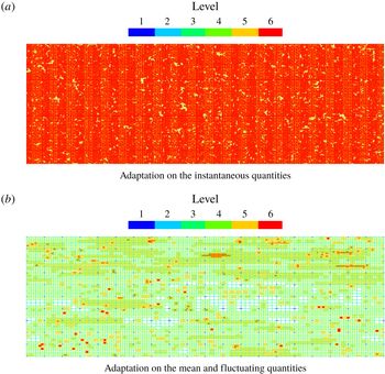
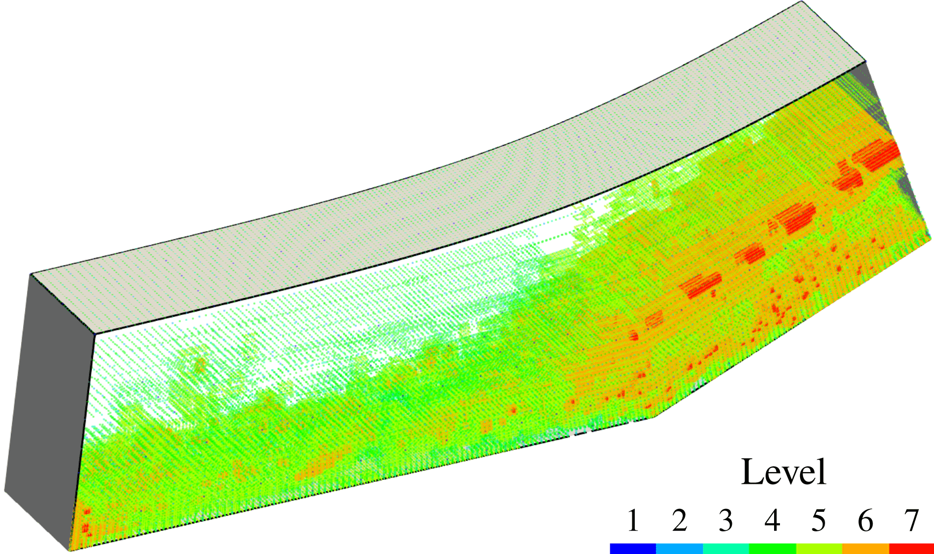
Adaptive grids points coloured by resolution levels at the solid wall. Horizontal direction is the streamwise direction and the vertical direction is the spanwise direction.

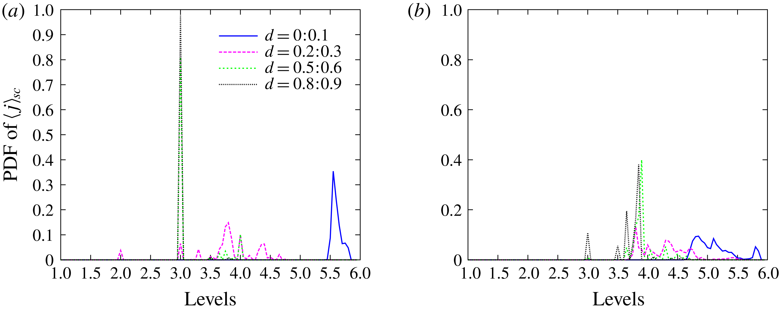
Probability density functions of spatially averaged grid levels
 $j_{sc}$
within four cuboidal subdomains at different wall distances. The lengths of the cuboidal subdomains in the
 $x$
and
 $z$
directions are
 $0.2H$
and the wall distance ranges of the cuboidal subdomains in the
 $y$
direction are
 $[0,0.1]H$
,
 $[0.2,0.3]H$
,
 $[0.5,0.6]H$
and
 $[0.8,0.9]H$
, respectively. (a) Probability density function of
 $j_{sc}$
for adaptation on the instataneous quantities corresponding to figure 1(a). (b) Probability density function of
 $j_{sc}$
for adaptation on the mean and fluctuating quantities corresponding to figure 1(b).

A supersonic turbulent channel flow case with the wavelet-based adaptive DDES method described above using the new adaptation procedure is tested. The effect of this adaptation procedure is illustrated in figures 1 and 2. Adaptive grid points coloured by resolution levels at the solid wall by different adaptation strategies are depicted in figure 1. Note that adapted quantities are momentum components, total energy and temperature. Since momentum and temperature are constant at the wall, perturbations exist only in the total energy that contains the density. Instantaneous quantities in figure 1(a) and mean quantities in figure 1(b) use
 $\bar{\unicode[STIX]{x1D716}}_{RANS}=2.5\times 10^{-3}$
and
 $\bar{\unicode[STIX]{x1D716}}_{LES}=5.0\times 10^{-2}$
. For the fluctuation fields in figure 1(b), increased thresholds
 $\unicode[STIX]{x1D716}_{RANS}^{\prime }=1.25\times 10^{-2}$
and
 $\unicode[STIX]{x1D716}_{LES}^{\prime }=2.5\times 10^{-1}$
are prescribed for testing purpose. Figure 1(a) has substantially more grid points retained at the wall than figure 1(b), while the total number of active grid points for the former is 3.2 million, it is 2.2 million for the latter.
The two grid adaptation strategies are also demonstrated in figure 2. Four cuboidal subdomains are sampled with lengths in the
 $x$
and
 $z$
directions equal to
 $0.2H$
and the wall distance ranges in the
 $y$
direction being
 $[0,0.1]H$
,
 $[0.2,0.3]H$
,
 $[0.5,0.6]H$
and
 $[0.8,0.9]H$
, respectively, where
 $H$
is the half-height of the channel. Levels of all adaptive grid points within these domains are averaged using the weighted average given by
 $$\begin{eqnarray}j_{sc}=\frac{\displaystyle \mathop{\sum }_{1\leqslant j\leqslant J}n_{j}j}{\displaystyle \mathop{\sum }_{1\leqslant j\leqslant J}n_{j}},\end{eqnarray}$$
where
 $n_{j}$
is the number of grid points on level
 $j$
. Since the computational grid is dynamically adapted,
 $j_{sc}$
is a function of time. The probability density functions of
 $j_{sc}(t)$
at four different wall distances for one domain flow-through time are plotted in figure 2. The considerable reduction of grid points at higher levels of resolution is evidenced by significantly lower probability density functions (PDF) for the near-wall RANS region shown in figure 2(b) compared to the height level spike observed in figure 2(a). In the middle part of the channel the grid points are mostly distributed on levels 3 and 4 for both cases, while figure 2(b) shows more grid points on higher levels of resolution.
Considering the mean and fluctuating components separately with different levels of effective wavelet filter threshold is thereby beneficial to retain the accuracy and gain the efficiency. This is justified by the fact that only the near-wall RANS region is remarkably coarsened by the split adaptation strategy on the mean and fluctuating components while the LES region is only slightly better resolved. As the solution becomes statistically converged, the averaged fields are smoother. Consequently, a smaller wavelet threshold for mean flow quantities can be used. Furthermore, the RANS model dissipation of small eddies entering from LES region and the dynamic mesh adaptation that guarantees adequate resolution of the penetrating eddies justify the use of higher threshold values for the fluctuating component in the RANS region, effectively spreading the resolved Reynolds stress between regions, improving model prediction and ensuring physically consistent model transition between the RANS and LES regions.
For statistically stationary flows that are only considered in this paper, it is natural to use the proposed split adaptation strategy on the mean and fluctuating components throughout the domain. However for statistically unsteady or statistically quasi-periodic flows the split mesh adaptation strategy can still be employed either in the entire domain or only in RANS regions. In the former case, for the problems with great disparity of large-scale unsteadiness and turbulence time scales, the split adaptation can use moving time-averaged fields. For problems without clear separation of time scales the split adaptation strategy can still be employed in the near-wall region, while the away from the wall, i.e. in LES regions, the adaptation on instantaneous quantities can be used. Also note that the main objective of split adaptation strategy is to have more precise control of the relative resolution of fluctuating components using more physically relevant scales based on the turbulence intensity instead of relying on instantaneous or mean flow scales. Thus, for problems, where statistically steady or slowly varying mean flow fields can not be determined, an alternative split adaptation strategy based on large and small-scale separation can be used. This alternative split adaptation strategy can be easily implemented utilizing level-based wavelet projection.
The details of the simulation set-up and results are presented below in § 5. One may argue here that DDES is known to be inappropriate for plane channel flow cases due to the log-layer mismatch (LLM) (Spalart et al. Reference Spalart, Deck, Shur, Squires, Strelets and Travin2006; Shur et al. Reference Shur, Spalart, Strelets and Travin2008) for attached flows. However, as stated above, the task of the current work is to investigate the coexistence of W-URANS and adaptive LES. Moreover, as demonstrated by results in the following section, the W-DDES method performs well for both attached and separated flows, while the conventional DDES usually fails for the former.
5 Simulations and results
5.1 Supersonic channel flow
In this subsection, simulations of supersonic channel flow for two different configurations are presented for testing of the wavelet-based DDES turbulence modelling approach and the novel grid adaptation strategy described in § 4. Fourth-order wavelets and finite difference scheme are used for the discrete wavelet transform and interpolation, and derivative approximations. For the time integration, the explicit standard four-stage Runge–Kutta scheme is applied with the CFL
 $=0.5$
. The grid adaptation is performed on mean (Reynolds-averaged) and fluctuating components of momentum, total energy and temperature scaled by
 $L_{2}$
norm. Specifically, the three components of momentum share a single scale that is calculated by the corresponding mean and fluctuation momentum magnitudes rather than using the scale of each individual component in the
 $x$
,
 $y$
and
 $z$
directions, respectively. The fluctuations of the total energy and temperature are evaluated by the Reynolds fluctuation root mean square. The wavelet filter thresholds for the mean quantities are
 $\bar{\unicode[STIX]{x1D716}}_{RANS}=2.5\times 10^{-3}$
and
 $\bar{\unicode[STIX]{x1D716}}_{LES}=5.0\times 10^{-2}$
, while larger thresholds
 $\unicode[STIX]{x1D716}_{RANS}^{\prime }=1.25\times 10^{-2}$
and
 $\unicode[STIX]{x1D716}_{LES}^{\prime }=2.5\times 10^{-1}$
are prescribed for all fluctuating quantities.
The wavelet thresholds for adaptation on the mean RANS and LES components were taken from the recommended ranges of wavelet thresholds in the adaptive LES and W-URANS methods for the adaptation strategy based on instantaneous flow variables. They are, respectively,
 $\unicode[STIX]{x1D716}_{LES}\sim O(10^{-2}-10^{-1})$
(Nejadmalayeri et al.
Reference Nejadmalayeri, Vezolainen, De Stefano and Vasilyev2014; Brown-Dymkoski Reference Brown-Dymkoski2016; De Stefano et al.
Reference De Stefano, Nejadmalayeri and Vasilyev2016) and
 $\unicode[STIX]{x1D716}_{RANS}\sim O(10^{-3})$
(De Stefano et al.
Reference De Stefano, Vasilyev and Brown-Dymkoski2018; Ge et al.
Reference Ge, Vasilyev, De Stefano and Hussaini2018). As explained in § 4 the choice of relatively high values of
 $\unicode[STIX]{x1D716}_{LES}^{\prime }$
and
 $\unicode[STIX]{x1D716}_{RANS}^{\prime }$
is justified by the RANS model dissipation of small eddies entering from the LES region and the dynamic mesh adaptation providing adequate resolution of the penetrating eddies. The selection of optimal values of wavelet thresholds balancing the accuracy and the computational efficiency varies for different flows and remains an open question for future study. The sensitivity of the solutions to the values of threshold
 $\unicode[STIX]{x1D716}$
is discussed later in this section.
An exponentially weighted time-average method is employed instead of the simple ensemble average during the early transient stage. For efficient computations, this may allow for calculations of the mean and fluctuating quantities and switching to the split adaptation relatively earlier than the solution becoming statistically converged. After statistical convergence, the Reynolds-average fields could be either exponentially weighted time averaged or ensemble averaged depending on how long the time period is over which the Reynolds-average fields would converge in different flow configurations. For example, for a channel flow where both streamwise and spanwise directions are homogeneous, the statistical sampling time may be shorter and the exponentially weighted time average is applicable. For flows with massive separation and high levels of unsteadiness, the sampling time should be longer and the ensemble average is more appropriate. Also note that for statistically unsteady or statistically quasi-periodic flows, an exponential time averaging can be interpreted as a moving time average.
Given an instantaneous quantity
 $\unicode[STIX]{x1D719}$
, the corresponding Reynolds-average quantity is denoted as
 $\langle \unicode[STIX]{x1D719}\rangle$
, which reads
 $$\begin{eqnarray}\langle \unicode[STIX]{x1D719}\rangle (t)\equiv \int _{-\infty }^{t}\unicode[STIX]{x1D719}(t^{\prime })\frac{1}{t_{s}}\text{e}^{-(t-t^{\prime })/t_{s}}\,\text{d}t^{\prime }.\end{eqnarray}$$
Differentiating equation (5.1) gives
 $$\begin{eqnarray}{\displaystyle \frac{\text{d}\langle \unicode[STIX]{x1D719}\rangle }{\text{d}t}}=\frac{1}{t_{s}}(\unicode[STIX]{x1D719}-\langle \unicode[STIX]{x1D719}\rangle ).\end{eqnarray}$$
Using a first-order approximation, equation (5.2) can be numerically evaluated as
 $$\begin{eqnarray}\left.\begin{array}{@{}c@{}}\displaystyle \langle \unicode[STIX]{x1D719}\rangle ^{n}=\unicode[STIX]{x1D6FC}\unicode[STIX]{x1D719}^{n}+(1-\unicode[STIX]{x1D6FC})\langle \unicode[STIX]{x1D719}\rangle ^{n-1},\\ \displaystyle \unicode[STIX]{x1D6FC}={\displaystyle \frac{\unicode[STIX]{x0394}t}{\unicode[STIX]{x0394}t+t_{s}}},\end{array}\right\}\end{eqnarray}$$
where
 $\unicode[STIX]{x0394}t$
is the time integration interval and
 $t_{s}$
is the time scale for the averaging. For the present channel flow case 10 % of one flow-through time (FTT),
 $t_{FTT}$
, is used for
 $t_{s}$
. A certain Reynolds fluctuating quantity is referred to as
 $\unicode[STIX]{x1D719}^{\prime }=\unicode[STIX]{x1D719}-\langle \unicode[STIX]{x1D719}\rangle$
. A Favre-average quantity is denoted as
 $\{\unicode[STIX]{x1D719}\}=\langle \unicode[STIX]{x1D70C}\unicode[STIX]{x1D719}\rangle /\langle \unicode[STIX]{x1D70C}\rangle$
while the corresponding Favre fluctuating variable is denoted as
 $\unicode[STIX]{x1D719}^{\prime \prime }=\unicode[STIX]{x1D719}-\{\unicode[STIX]{x1D719}\}$
.
The computational domain size is
 $4\unicode[STIX]{x03C0}H\times 2H\times 4\unicode[STIX]{x03C0}H/3$
in the streamwise(
 $x$
), wall-normal(
 $y$
) and spanwise(
 $z$
) directions, respectively, where
 $H$
is the half-height of the channel. The bulk Reynolds number is
 $Re=\unicode[STIX]{x1D70C}_{b}u_{b}H/\unicode[STIX]{x1D707}_{w}$
, and the Mach number is
 $Ma=u_{b}/c_{w}$
, where
 $(\cdot )_{b}$
and
 $(\cdot )_{w}$
, respectively, denote bulk mean quantities and quantities averaged at the walls, while
 $c$
is the speed of sound. The friction Reynolds number is
 $Re_{\unicode[STIX]{x1D70F}}=\unicode[STIX]{x1D70C}_{w}u_{\unicode[STIX]{x1D70F}}H/\unicode[STIX]{x1D707}_{w}$
, where
 $u_{\unicode[STIX]{x1D70F}}=\sqrt{\unicode[STIX]{x1D70F}_{w}/\unicode[STIX]{x1D70C}_{w}}$
. Here,
 $\unicode[STIX]{x1D70F}_{w}$
indicates the wall shear stress. Two flow configurations i.e.
 $Re=3000$
with
 $Ma=1.5$
and
 $Re=6000$
with
 $Ma=3.0$
are considered. No-slip and isothermal boundary conditions are imposed on the walls and periodicity is assumed in the streamwise and spanwise directions. A feedback control of the body force in the streamwise direction based on the bulk mass flow rate is employed to maintain the desired flow rate. Once the statistically steady state regime is achieved, the feedback is turned off and the statistics start to be recalculated. The initial conditions are: the laminar parabolic velocity profile for plane channel flow, uniform density and total energy. Initial condition for
 $\tilde{\unicode[STIX]{x1D708}}$
has a prescribed value at the wall and exponentially approaches to a uniform value in the free stream. In order to accelerate the transition to fully developed turbulence, the least stable modes of the two-dimensional Orr–Sommerfeld solution are superimposed as velocity perturbations in the
 $x$
and
 $y$
directions along with smooth random noises in the
 $y$
and
 $z$
directions.
The discretization of the computational domain is done by using dyadic nested wavelet collocation grids for the wavelet decomposition (3.2). For the
 $Re=3000$
and
 $Ma=1.5$
case, the computational mesh has
 $J=6$
and an effective (finest level) resolution of
 $640\times 224\times 320$
with base (coarsest level) grids with resolution of
 $20\times 7\times 10$
. Using A-AWCM, the mesh is stretched in the wall-normal direction following a hyperbolic tangent distribution. For the finest level of resolution, the first wall-normal grid spacing is
 $\unicode[STIX]{x0394}y(1)^{+}=0.29$
with a corresponding stretching ratio equal to 1.04. The
 $x$
and
 $z$
directions have periodic boundary conditions with grid points evenly distributed. The grid aspect ratios in the immediate vicinity of the wall are
 $\unicode[STIX]{x0394}x^{+}/\unicode[STIX]{x0394}y^{+}=15$
and
 $\unicode[STIX]{x0394}z^{+}/\unicode[STIX]{x0394}y^{+}=10$
. The curvilinear mapping and the resulting grid aspect ratios for the physical grid coordinates are determined a priori. In the LES region away from the wall, where the turbulent structures become more isotropic, the aspect ratios approach the order of unity. These configurations of grid aspect ratios are typical for wall-bounded LES or hybrid URANS/LES computations. Similar set-ups hold for all simulations contained in this paper. The grid compression ratio, defined as the percentage of collocation points discarded in the adaptive grid (2.5 million) compared to the number of underlying non-adaptive grid points is 95.0 %. An adaptive LES study (Brown-Dymkoski Reference Brown-Dymkoski2016) for the same channel flow case has active grid points of 3.5 million with an aggressive uniform threshold
 $\unicode[STIX]{x1D716}=0.1$
adapting to instantaneous momentum, total energy and temperature. Both the accuracy indicated by the threshold and efficiency in terms of degrees of freedom for the novel adaptation strategy are successfully achieved.
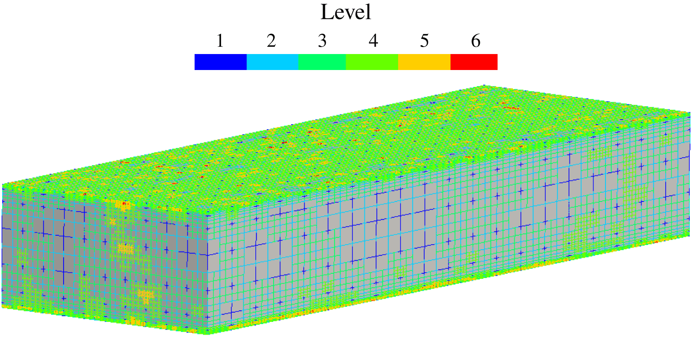
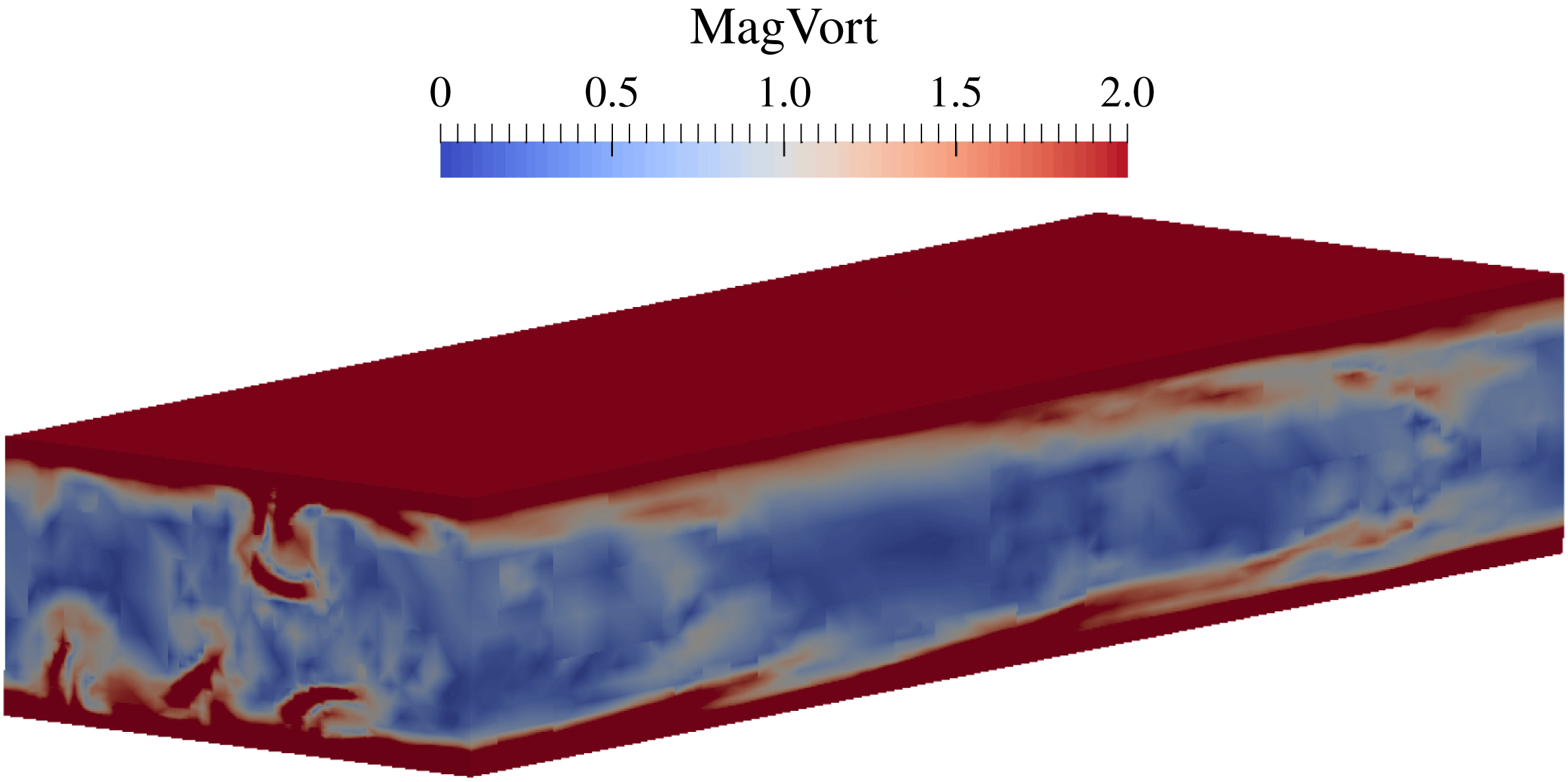
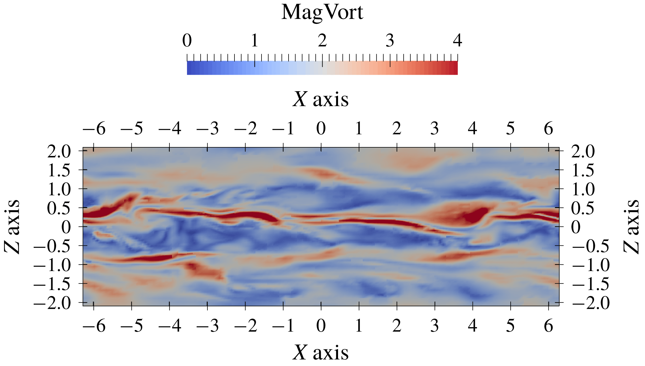
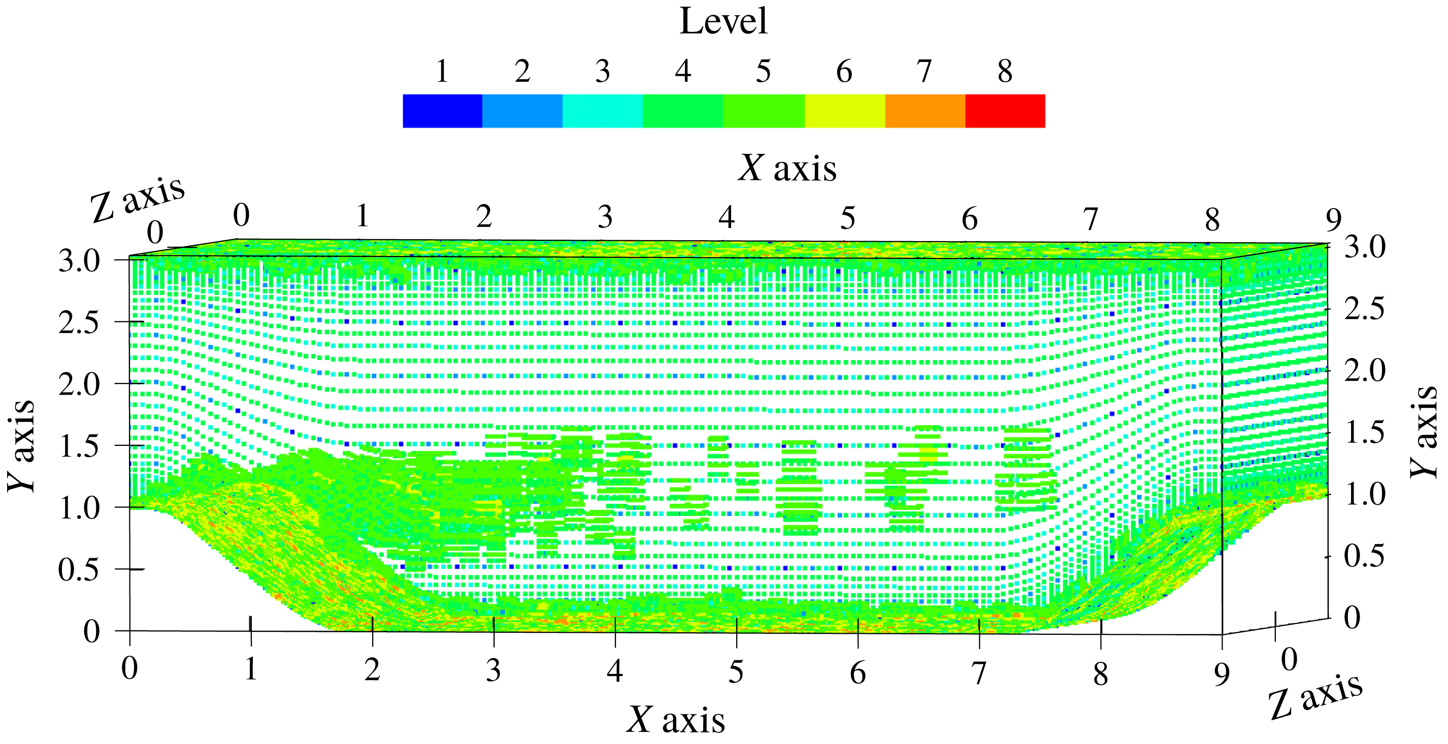
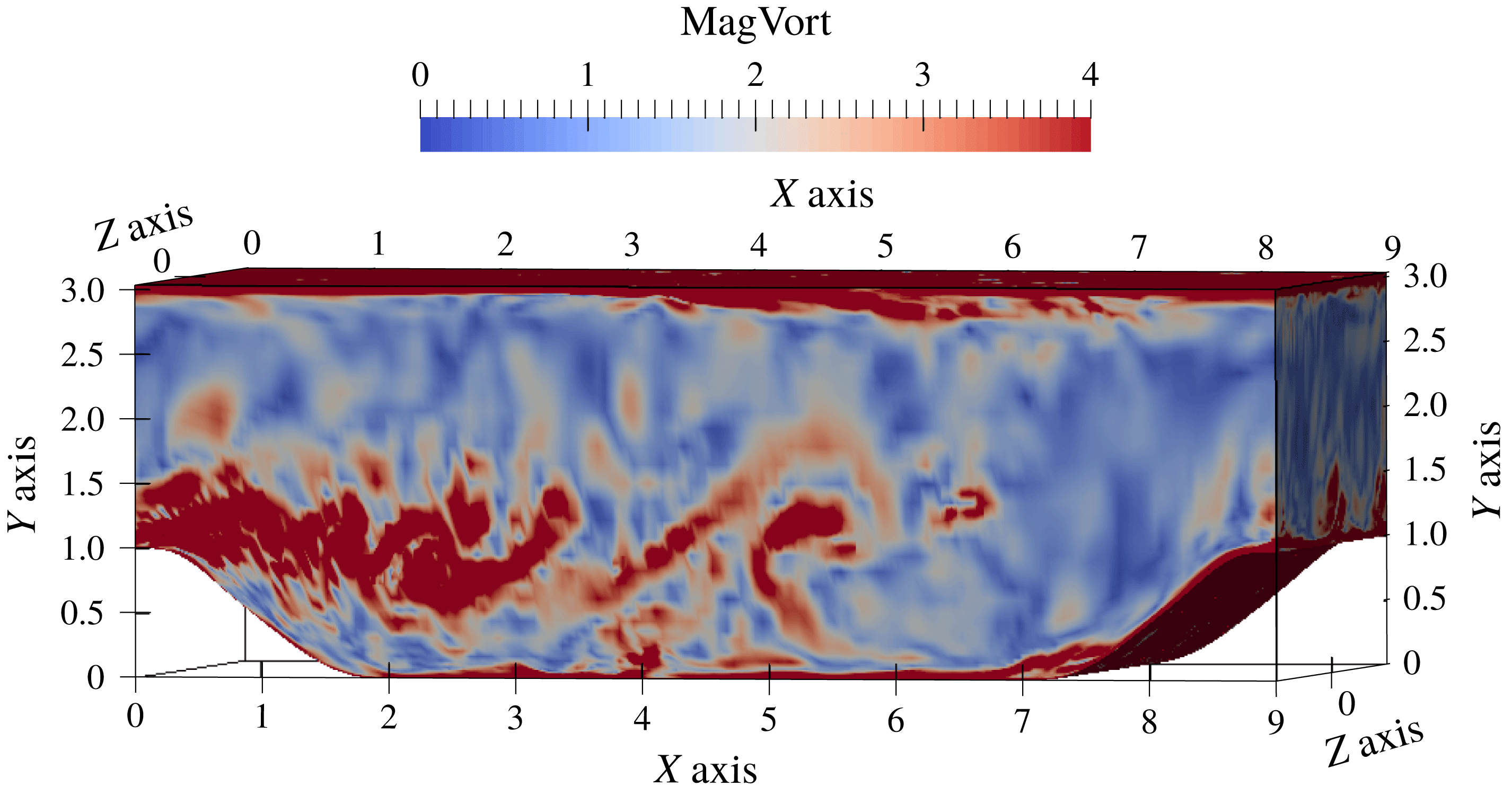
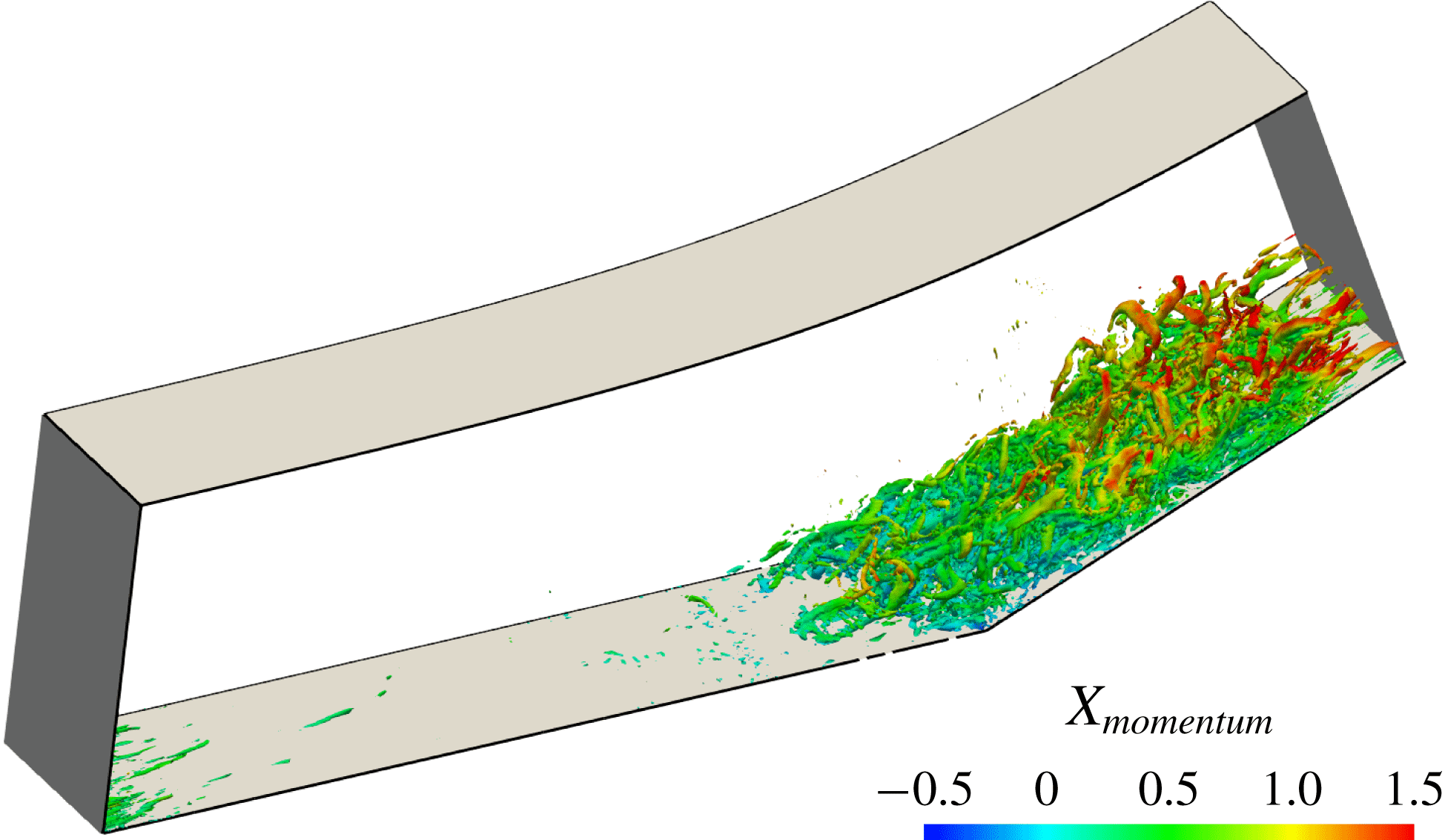
The adaptive grid for the developed turbulent flow field is illustrated in figure 3, demonstrating refinement around localized structures visualized by the vorticity magnitude contours in figure 4. The mean and turbulence statistics profiles are plotted in figures 5–11. Statistics are computed by interpolating the continuous wavelet basis onto two-dimensional (2-D) non-adaptive sampling grids, and averaging along the streamwise direction in each 2-D slice and then across multiple slices over a long time period with exponentially decaying weights. Therefore all curves plotted below show the streamwise, spanwise and time-averaged quantities of the W-DDES solution. Due to the high Mach number and iso-thermal boundary condition, the temperature within the channel increases because of the viscous dissipation heating. It appears that the thermodynamic related quantities, namely the density and total energy, converge more slowly than the momentum.
The adaptive grids on the surfaces of the physical domain.

The instantaneous vorticity magnitude contours on the surfaces of the physical domain.

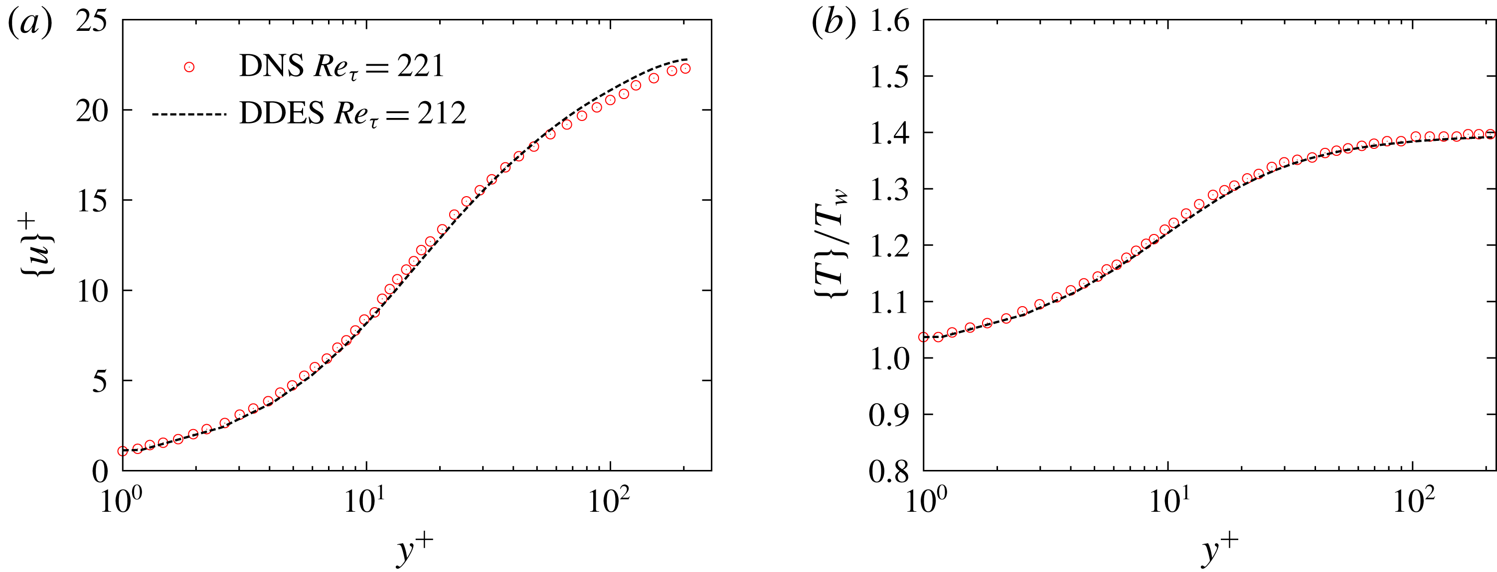
Mean profile comparison between W-DDES and DNS results for the plane channel flow case with
 $Re=3000$
and
 $Ma=1.5$
. (a) Velocity profiles. DNS data from Coleman, Kim & Moser (Reference Coleman, Kim and Moser1995). (b) Temperature profiles. DNS data from Morinishi, Tamano & Nakabayashi (Reference Morinishi, Tamano and Nakabayashi2004).

The friction Reynolds number
 $Re_{\unicode[STIX]{x1D70F}}$
predicted by the W-DDES is 212, a 4.0 % underestimate compared with the benchmark DNS results (Coleman et al.
Reference Coleman, Kim and Moser1995; Foysi, Sarkar & Friedrich Reference Foysi, Sarkar and Friedrich2004; Morinishi et al.
Reference Morinishi, Tamano and Nakabayashi2004) at
 $Re_{\unicode[STIX]{x1D70F}}=221$
. Two sources exist for this error. The first is the
 $\unicode[STIX]{x1D716}_{hyb}$
for the mean quantities. The second is the LLM issue of DDES, where the intersection of the log-law velocity profiles predicted in the LES regime of the DDES model is higher than that in the RANS regime, although both regimes share the same log-law slope. This issue may introduce an underestimation of the friction of up to 15 % (Spalart et al.
Reference Spalart, Deck, Shur, Squires, Strelets and Travin2006). However, our predicted
 $Re_{\unicode[STIX]{x1D70F}}$
is obviously much better than a typical LLM result by the conventional DDES. In fact, it is even better than the result of the wavelet-based adaptive wall-resolved LES at
 $Re_{\unicode[STIX]{x1D70F}}=205$
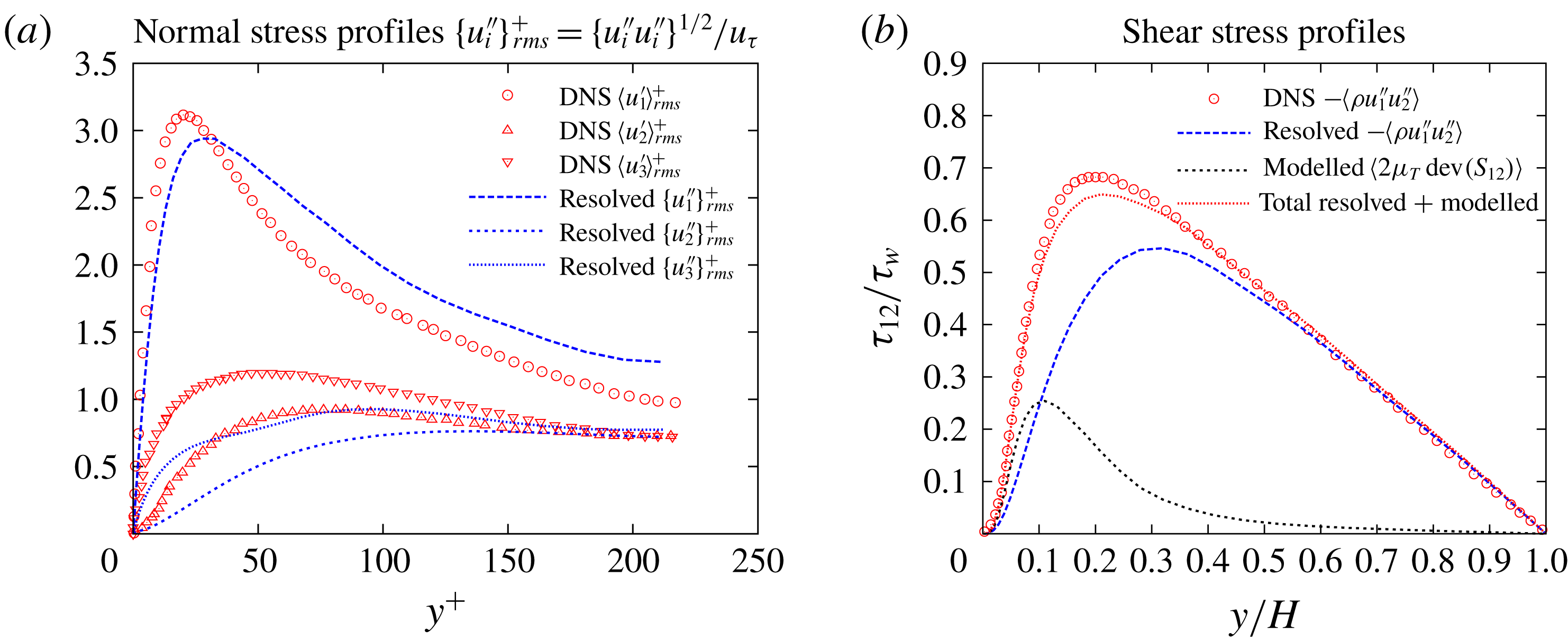
as reported in Brown-Dymkoski (Reference Brown-Dymkoski2016). Moreover, the Reynolds mean velocity and temperature profile shown in figure 5 agree quite well with the DNS data. The LLM is significantly mitigated by an overestimation of the resolved part of the turbulent normal stress
 $\{u_{1}^{\prime \prime }\}_{rms}$
as plotted in figure 6(a). This can be explained by the benefit of the wavelet-based adaptation where the local mesh refinement in the LES region results in high levels of resolved turbulent stresses, and hence more momentum can be transported into the lower portion of the boundary layer. On the contrary, the conventional non-adaptive DDES predicts relatively low levels of resolved turbulent stresses, while it excessively damps out turbulence at the RANS–LES interface, located at the log-law region. Meanwhile, both tangential normal stresses
 ${u_{1}^{\prime \prime }}_{rms}$
and
 ${u_{3}^{\prime \prime }}_{rms}$
and transverse normal stress
 ${u_{2}^{\prime \prime }}_{rms}$
are underestimated around and below the RANS–LES interface as shown in figure 6(a), which is the intrinsic feature of the DDES model, whereas the LES mode is shielded below the log layer. Note that the DNS normal stresses compared are the Reynolds-averaged fluctuations instead of the Favre-averaged ones. However, their differences are negligible since they originate from high order and triple correlation terms (Morinishi et al.
Reference Morinishi, Tamano and Nakabayashi2004).
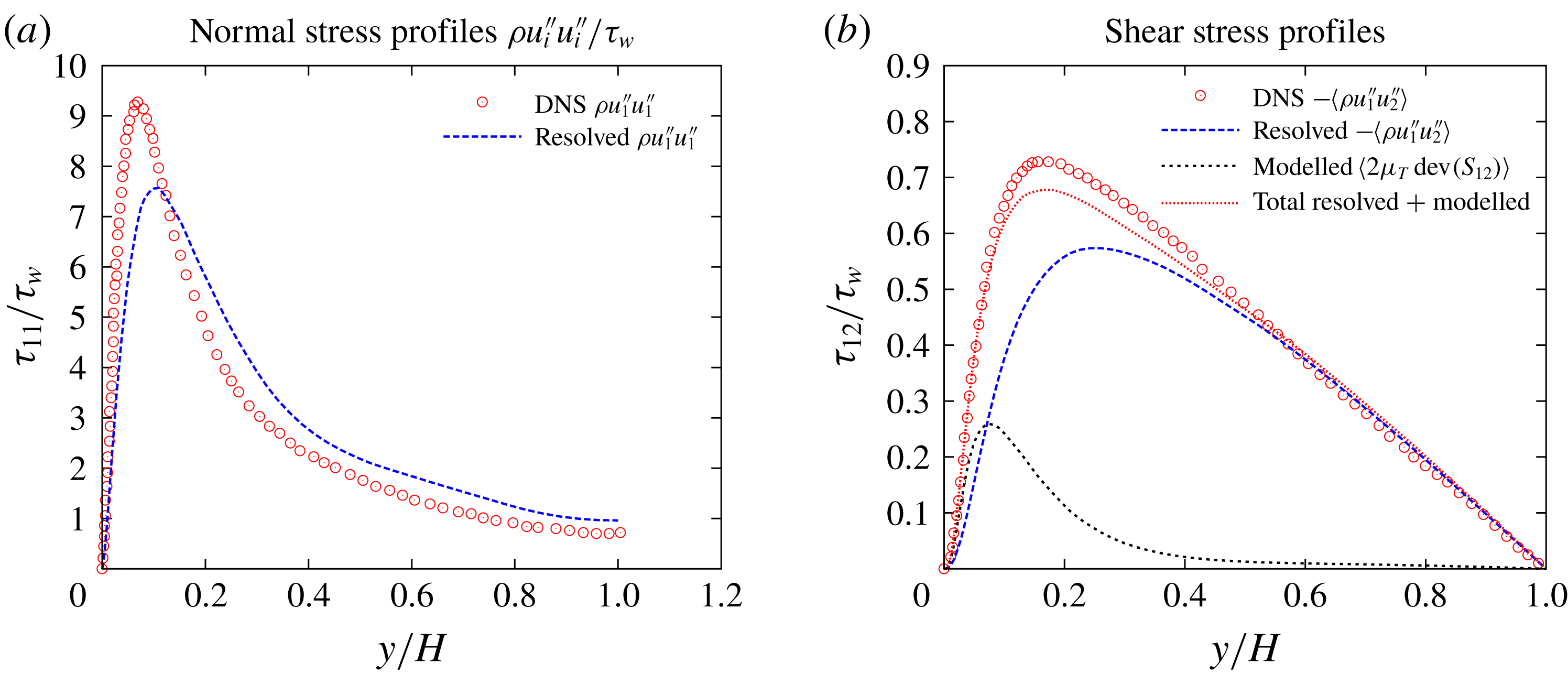
Turbulent stresses profiles comparison between W-DDES and DNS results for the plane channel flow case with
 $Re=3000$
and
 $Ma=1.5$
. (a) Resolved turbulent normal stress profiles by DDES and comparison with the DNS data from Coleman et al. (Reference Coleman, Kim and Moser1995). (b) Resolved, modelled and total turbulent shear stress profiles by DDES and comparison with the DNS data from Foysi et al. (Reference Foysi, Sarkar and Friedrich2004).

From the perspective of the modelling terms, the benefit of the adaptive method is also seen. The local mesh refinement causes the reduction of the local sub-grid length scale
 $\unicode[STIX]{x1D6E5}$
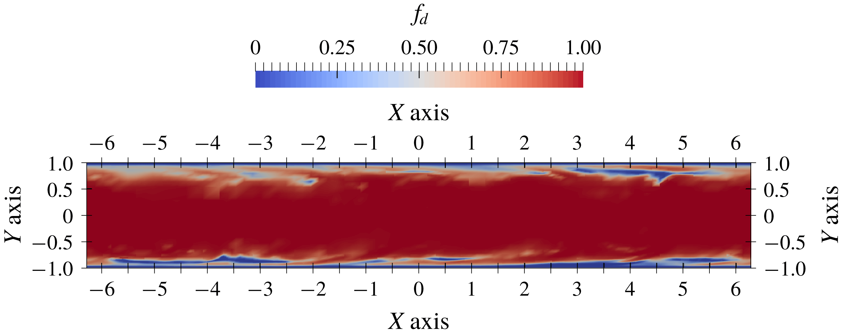
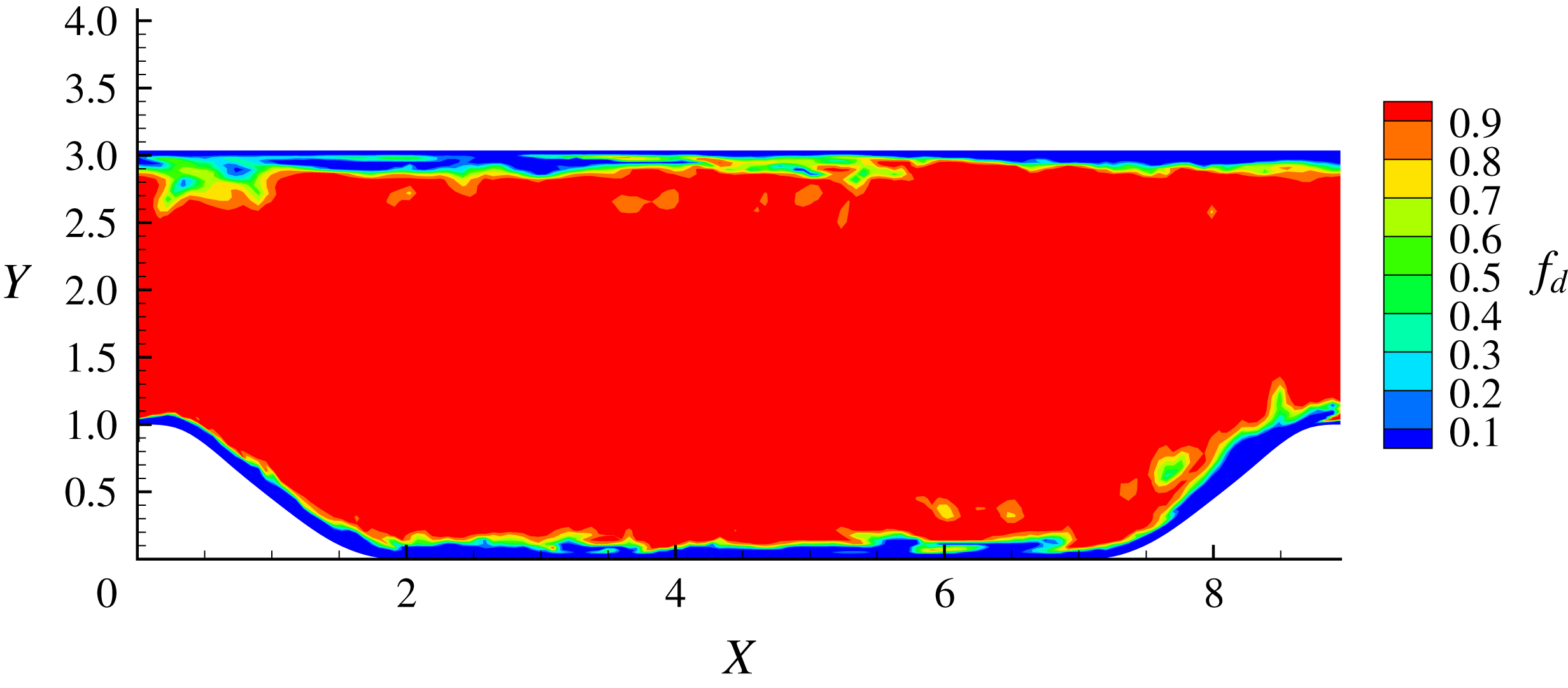
as in (2.12), i.e. the length scale for the LES regime. The idea of the DDES modelling is that the limiter of the length scale as in (2.11) has an effect of bounding of the eddy viscosity. Therefore, the local reduction of the LES length scale in turn reduces the local eddy viscosity and further enhances the resolved turbulent stresses. For the S–A based DDES model used in this paper, the instantaneous shielding function
 $f_{d}$
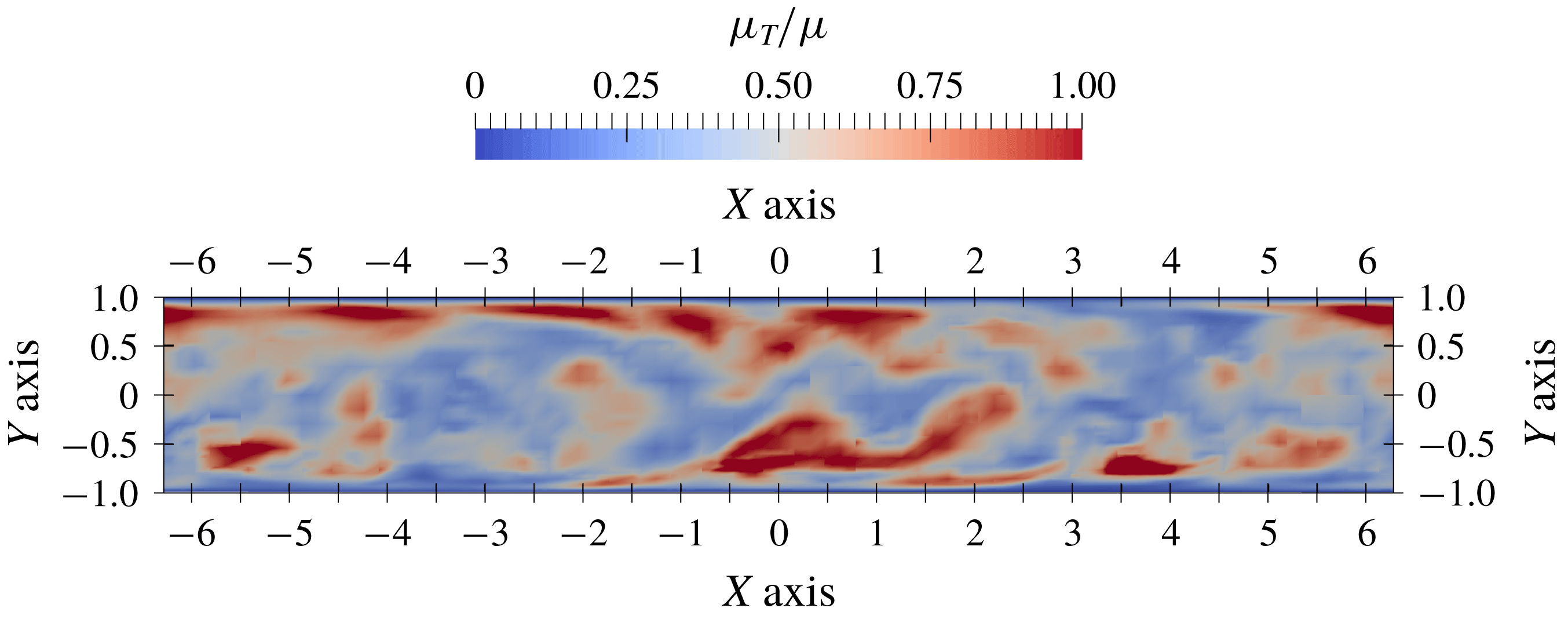
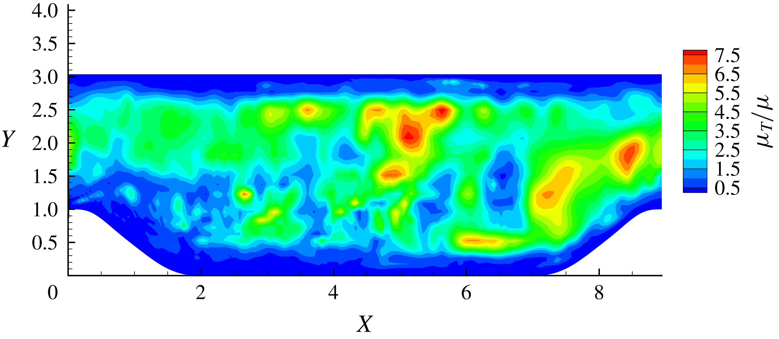
is able to increase locally due to the enhanced LES regime invoked by the adaptive mesh refinement. This is illustrated by the instantaneous contours of
 $f_{d}$
and the ratio of eddy viscosity to molecular viscosity
 $\unicode[STIX]{x1D707}_{T}/\unicode[STIX]{x1D707}$
displayed in figures 7 and 8. Wherever the resolved turbulence is enhanced indicated by high values of
 $f_{d}$
at the RANS–LES interface, the eddy viscosity is lower and vice versa.
The instantaneous
 $f_{d}$
contours in an
 $x$
–
 $y$
plane of the supersonic channel case. The blue regions represent the RANS regime and the red regions represent the LES regime.

The instantaneous
 $\unicode[STIX]{x1D707}_{T}/\unicode[STIX]{x1D707}$
contours in an
 $x$
–
 $y$
plane of the supersonic channel case.

The instantaneous vorticity magnitude contours in an
 $x{-}z$
plane with constant wall distance
 $0.2H$
.

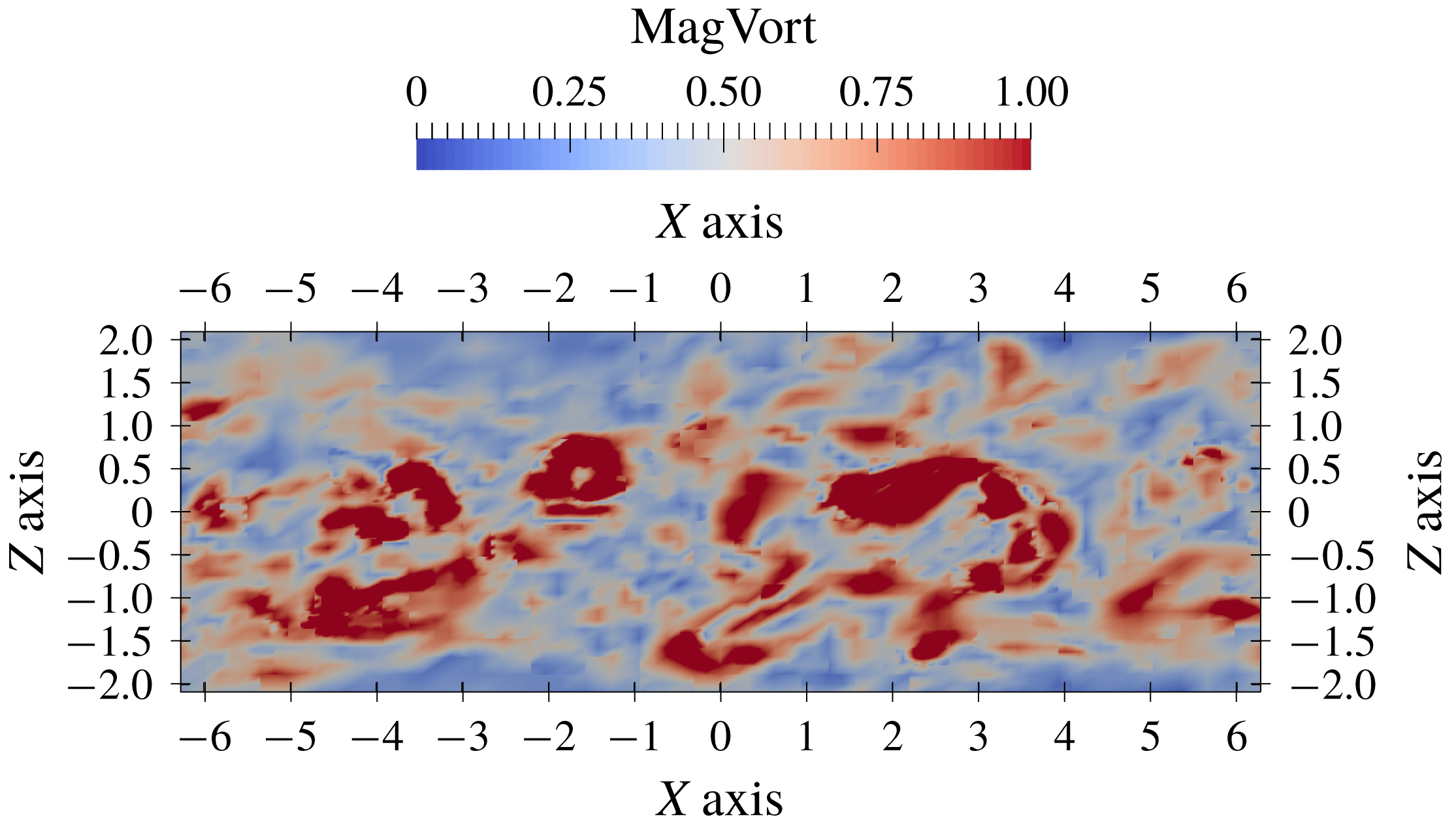
The instantaneous vorticity magnitude contours in an
 $x{-}z$
plane with constant wall distance
 $0.8H$
.

Figure 6(b) depicts the resolved, modelled and total turbulent shear stress
 $-\langle \unicode[STIX]{x1D70C}u_{1}^{\prime \prime }u_{2}^{\prime \prime }\rangle$
compared with the DNS data. Note that modelled normal stresses are negligible in figure 6(a) because of the small mean velocity gradient
 $\unicode[STIX]{x2202}_{x}\langle u_{i}\rangle$
. Similar to the turbulent normal stresses, the predicted shear stress is slightly underestimated around the RANS–LES interface layer where
 $y^{+}\approx 20$
–50. In addition, the predicted peak of the maximum value of the turbulent normal stress component shown in figure 6(a) is slightly closer to the middle of the channel than in the DNS data. Figures 9 and 10 visualize the instantaneous vorticity magnitude at the RANS–LES interface and near the middle of the channel, respectively. The smooth elongated streaks shown in figure 9 are similar to the convectional DDES results, as opposed to the ‘improved DDES’ (IDDES) results presented in Shur et al. (Reference Shur, Spalart, Strelets and Travin2008) with much smaller eddy structures. From these observations, the issue of damping of turbulence at the RANS–LES interface for conventional low resolution non-adaptive DDES still exists. At the away-wall region shown in figure 10, the eddy structures are isotropic and similar to both conventional DDES and IDDES.
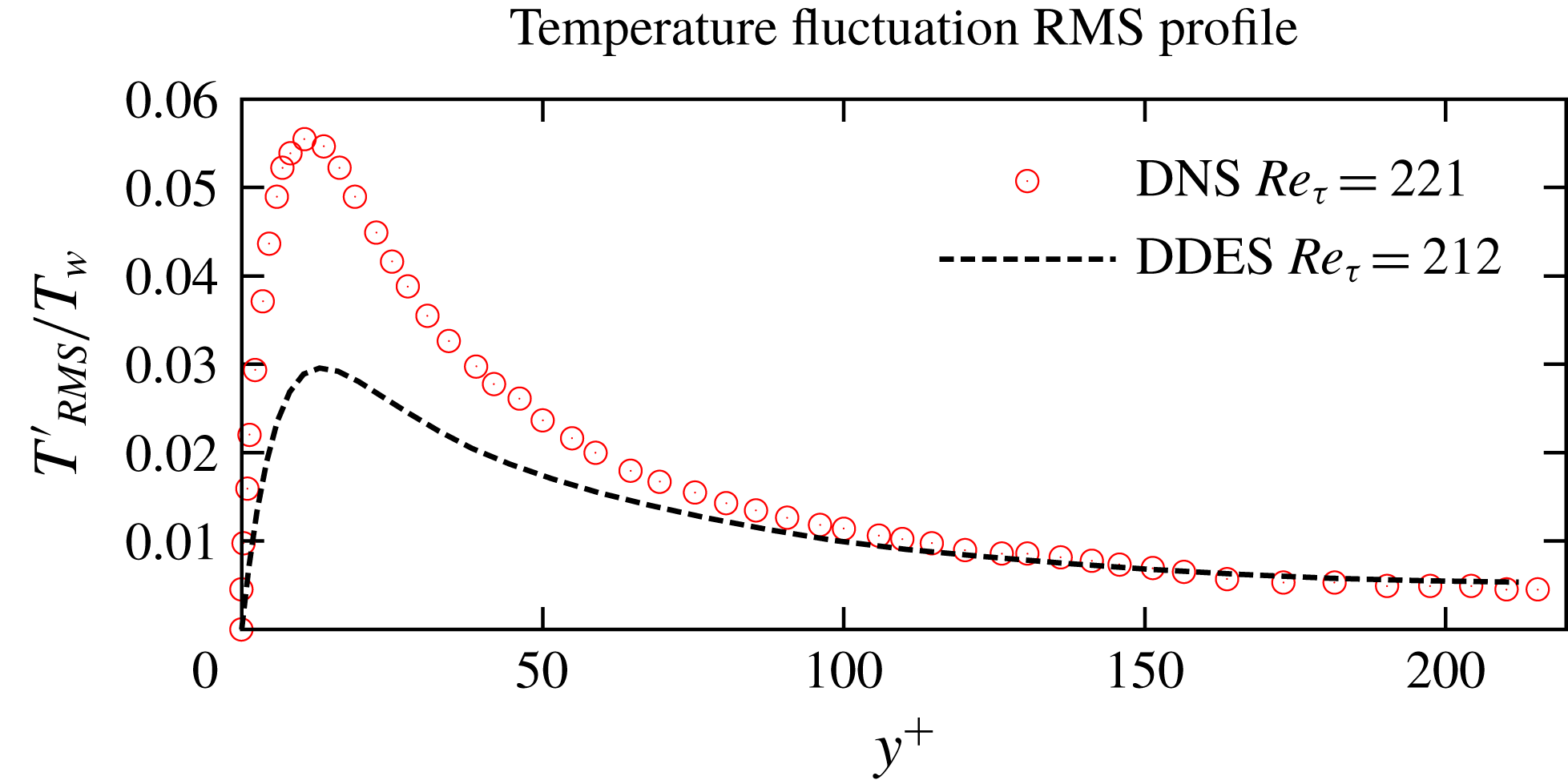
Reynolds fluctuation root mean square of the temperature field and comparison with the DNS data (Morinishi et al. Reference Morinishi, Tamano and Nakabayashi2004).

The Reynolds fluctuation root mean square temperature profiles plotted in figure 11 illustrate an underestimation of temperature fluctuation compared with the DNS data. Note that the turbulent heat flux is modelled through a Reynolds analogy as in (2.6) with a constant turbulent Prandtl number,
 $Pr_{T}=0.9$
; the temperature fluctuations are not well modelled, as opposed to the eddy viscosity and the Reynolds stresses. So the result in figure 11 is acceptable. The fact that we partially resolve the temperature fluctuations makes the approach closer to LES than RANS where the fluctuation should be zero.
As argued in § 4, the current work aims to show the capability of the coexistence of the W-RANS and adaptive LES regimes within the A-AWCM framework. Our results successfully demonstrate the feasibility of the novel W-DDES modelling approach proposed in this work.
It is worth emphasizing the importance of using the time-averaged absolute wavelet thresholding scale
 $\Vert u\Vert$
used in (3.2) to ensure its smooth variation in time. Turbulent fluctuations are highly intermittent in nature. As a result, the instantaneous scales of the fluctuating components also vary in time. A rapid increase of the absolute thresholding scale could result in excessive filtering of turbulent fluctuations in the LES region and the expansion of the RANS region, which, in turn, could manifest itself in the log-layer mismatch. In the simulation discussed above, the time-averaged scales given by the discrete version (5.3) of (5.2) are used to calculate the averaged absolute thresholding scales, with
 $t_{s}\approx 0.1t_{FTT}$
.
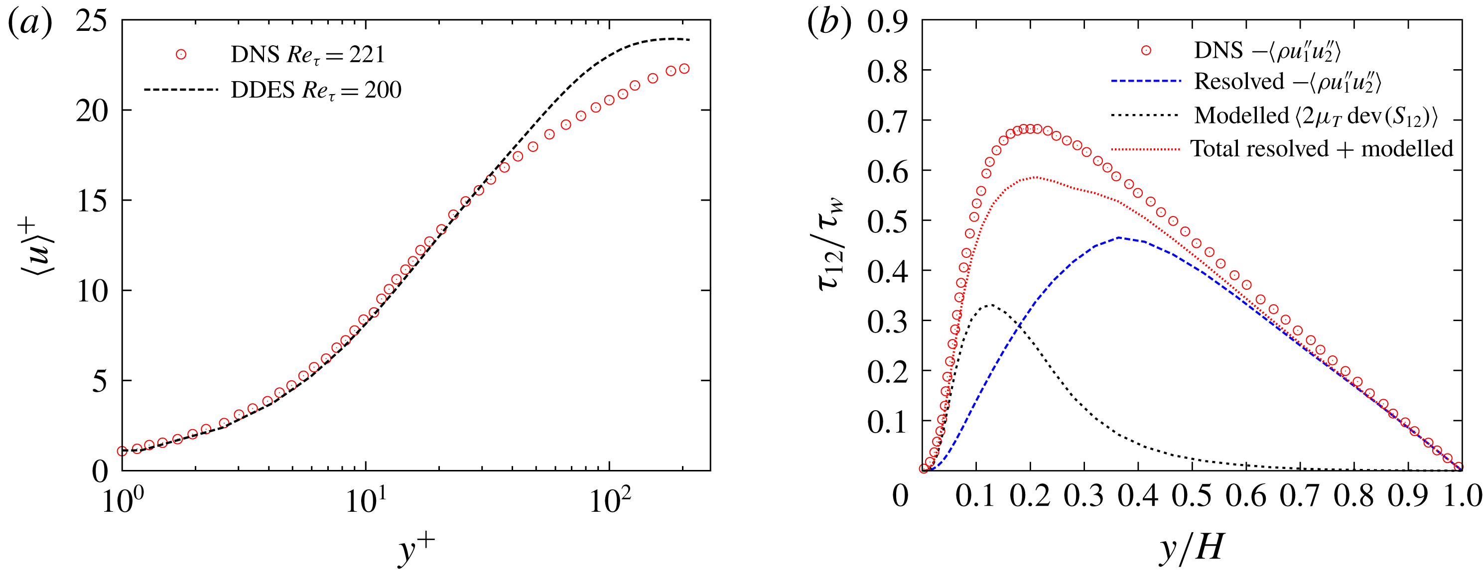
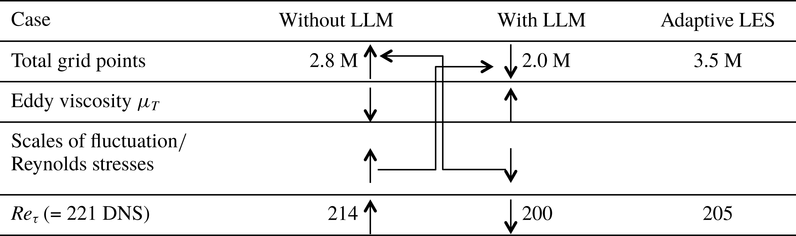
A possible appearance of the LLM solution when the instantaneous absolute thresholding scales are used is demonstrated in figure 12. The discrepancy of the mean streamwise velocity profiles is significant as shown in figure 12(a). The excessive filtering of fluctuating components in the LES region results in the under-resolution of turbulent shear stress as shown in figure 12(b), which causes an excessive underestimation of the total shear stress. It should be noted that when the instantaneous absolute thresholding scales are used, the solution switches between two branches: one with the LLM issue and the other without. Figure 13 shows the mechanism of the two-branch solutions when the instantaneous absolute thresholding scales are used. A typical LLM solution produces relatively higher values of eddy viscosity and lower values of resolved Reynolds stresses or fluctuations. Therefore the adaptive criterion of the wavelet coefficient based on the instantaneous fluctuating quantities is loosened and more grid points are retained. Meanwhile, more grid points, in turn, suppress the eddy viscosity and hence enhance the resolved Reynolds stresses, which finally leads to a more accurate solution without LLM. However, when the fluctuating components are increased, more grid points are discarded, resulting in coarsening of the adaptive grid and the solution is driven back to typical LLM branch. When time-averaged absolute thresholding scales are used, no LLM is observed and solutions for LES and RANS branches match and converge to the statistically steady solution presented in figures 5, 6 and 11.
Turbulent stresses profiles comparison between W-DDES with log-layer mismatch and DNS results. (a) Velocity profiles. DNS data from Coleman et al. (Reference Coleman, Kim and Moser1995). (b) Resolved, modelled and total turbulent shear stress profiles by DDES and comparison with the DNS data from Foysi et al. (Reference Foysi, Sarkar and Friedrich2004).

Schematic of the mechanism of the two-branch solutions when instantaneous quantity scales are used for wavelet filter thresholding. A typical LLM solution produces relatively higher values of eddy viscosity and lower values of resolved Reynolds stresses or fluctuations. Therefore the adaptive criterion of the wavelet coefficient based on the instantaneous fluctuating quantities is loosened and more grid points are retained. Meanwhile, more grid points, in turn, suppress the eddy viscosity and hence enhance the resolved Reynolds stresses, which finally leads to a more accurate solution without significant LLM. However, when the fluctuating components have increased, more grid points are discarded. This way the adaptive grid will be locally coarsened, and drive the solution back to typical LLM branch. The wavelet-based adaptive wall-resolved LES (adaptive LES) data from Brown-Dymkoski (Reference Brown-Dymkoski2016) as reference.

In order to further examine the grid convergence with regard to the sensitivity of the solutions to the values of the wavelet filter thresholds
 $\unicode[STIX]{x1D716}_{LES}$
and
 $\unicode[STIX]{x1D716}_{RANS}$
, three pairs of mean wavelet thresholds are compared: (i) low
 $\unicode[STIX]{x1D716}_{RANS}=1.5\times 10^{-3}$
and
 $\unicode[STIX]{x1D716}_{LES}=3.0\times 10^{-2}$
, (ii) medium
 $\unicode[STIX]{x1D716}_{RANS}=2.5\times 10^{-3}$
and
 $\unicode[STIX]{x1D716}_{LES}=5.0\times 10^{-2}$
and (iii) high
 $\unicode[STIX]{x1D716}_{RANS}=5.0\times 10^{-3}$
and
 $\unicode[STIX]{x1D716}_{LES}=1.0\times 10^{-1}$
. The wavelet threshold parameters for the fluctuating components in both LES and RANS regions are five times as large as the ones for the mean quantities.
Sensitivity tests of the solutions and grid sizes to the wavelet thresholds in the plane channel flow case at
 $Re=3000$
and
 $Ma=1.5$
with
 $Re_{\unicode[STIX]{x1D70F}}=221$
from the DNS (Foysi et al.
Reference Foysi, Sarkar and Friedrich2004) with a non-adaptive grid size of 3.7 million.

The resulting
 $Re_{\unicode[STIX]{x1D70F}}$
and adaptive grid sizes for different wavelet thresholds are summarized in table 1, where the results for the adaptive LES (Brown-Dymkoski Reference Brown-Dymkoski2016) are also given for comparison. The number of degrees of freedom for the adaptive LES is considerably larger than W-DDES simulations with the same
 $\unicode[STIX]{x1D716}_{LES}=0.1$
wavelet threshold, while the accuracy of the results in terms of
 $Re_{\unicode[STIX]{x1D70F}}$
is lower. The lower computational efficiency and less accurate results are mainly attributed to the global character of the mesh adaptation strategy, where the adaptation on instantaneous flow fields with global threshold
 $\unicode[STIX]{x1D716}=0.1$
was used. The use of a large global wavelet threshold with the absolute scales mainly determined by mean flow resulted in under-resolution and loss of accuracy in the wall region due to excessive filtering of small-scale structures, necessitating the use of smaller wavelet thresholds in the wall region as well as a clear separation of the mean and fluctuating flow components. In fact the study of Brown-Dymkoski (Reference Brown-Dymkoski2016) was the motivation to develop the novel adaptation strategy based on mean and fluctuating components which is reported in this paper. Also note that, even though the split adaptation strategy improves the computational efficiency of both adaptive LES and W-URANS, the requirement for the wall-resolved adaptive LES to use smaller wavelet threshold values (i.e. higher grid resolution) in the wall region demonstrates the necessity of developing the W-DDES or hybrid URANS/LES approach utilizing the adaptive wavelet-based method.
Sensitivity of the velocity and
 $f_{d}$
profiles to the wavelet thresholds in the channel flow case
 $Re=3000$
and
 $Ma=1.5$
. (a) Streamwise and spanwise and Favre-averaged velocity profiles. DNS data from Coleman et al. (Reference Coleman, Kim and Moser1995). (b) Streamwise and spanwise averaged instantaneous profiles of
 $f_{d}$
.

The results reported in table 1 and figure 14(a) confirm the expected increase of the accuracy of W-URANS simulations with the decrease of wavelet threshold values, although at the expense of increasing the size of the adaptive grid. It should be noticed that the results of the simulations are considerably less sensitive to the wavelet threshold values compared to the adaptive grid size. This may justify the use of relatively large values of
 $\unicode[STIX]{x1D716}$
for efficiency purposes. In fact, even the results for the high levels of thresholds
 $\unicode[STIX]{x1D716}_{RANS}=5.0\times 10^{-3}$
and
 $\unicode[STIX]{x1D716}_{LES}=1.0\times 10^{-1}$
are acceptable. This high threshold level set-up may be treated as the upper limit of the wavelet thresholds since further increase would lead to under-resolution and loss of accuracy for both the RANS and LES regimes.
The dynamic nature of the switching mechanism between the RANS and LES regimes is illustrated in figure 14 where the streamwise- and spanwise-averaged profiles of velocity and shielding function
 $f_{d}$
are shown for three
 $\unicode[STIX]{x1D716}$
configurations. Even though the medium
 $\unicode[STIX]{x1D716}$
, chosen for the original W-DDES computation presented above, displays adequately good agreement with the DNS results, the
 $f_{d}$
profiles with different levels of
 $\unicode[STIX]{x1D716}$
suggest that the switch from the RANS to LES regime occurs faster for the smaller
 $\unicode[STIX]{x1D716}$
. This is crucial to the success of the W-DDES and demonstrates that the increase of the accuracy of the solution is achieved by enhancing the resolved parts of the turbulent stresses from the LES side of the simulation.
Another plane channel flow case with
 $Re=6000$
with
 $Ma=3.0$
is also considered. The computational set-up for this case is very similar to the
 $Re=3000$
with
 $Ma=1.5$
case except that a finer mesh with the highest level
 $J=7$
is used. Therefore the effective (finest level) resolution becomes
 $1280\times 448\times 640$
with the same base (coarsest level) grids with resolution
 $20\times 7\times 10$
. The wavelet filter thresholds are the same as for the low
 $Re$
case, i.e. the mean quantities are
 $\unicode[STIX]{x1D716}_{RANS}=2.5\times 10^{-3}$
and
 $\unicode[STIX]{x1D716}_{LES}=5.0\times 10^{-2}$
, while to decrease the computational cost increased thresholds
 $\unicode[STIX]{x1D716}_{RANS}=1.25\times 10^{-2}$
and
 $\unicode[STIX]{x1D716}_{LES}=2.5\times 10^{-1}$
are used for the fluctuating components. The resulting grid compression ratio is approximately 98.85 % using an adaptive grid size of approximately 4.2 million. The friction Reynolds number
 $Re_{\unicode[STIX]{x1D70F}}$
predicted by the W-DDES using this
 $\unicode[STIX]{x1D716}$
field is 548, producing an error of 1.4 % compared with 556 predicted by DNS in Foysi et al. (Reference Foysi, Sarkar and Friedrich2004). Note that the result of the wall-resolved adaptive LES reported in Brown-Dymkoski (Reference Brown-Dymkoski2016) is
 $Re_{\unicode[STIX]{x1D70F}}=512$
with an adaptive grid size of 8.5 million. The corresponding mean velocity and density profiles are plotted in figure 15 and the turbulent shear stress
 $-\langle \unicode[STIX]{x1D70C}u_{1}^{\prime \prime }u_{2}^{\prime \prime }\rangle$
and streamwise normal stress
 $\langle \unicode[STIX]{x1D70C}u_{1}^{\prime \prime }u_{1}^{\prime \prime }\rangle$
are plotted in figure 16. Similar plots of the wall-normal and spanwise normal stress components are not given since the DNS data are not available for comparison. Fairly good agreements between the W-DDES results and the reference DNS data are obtained.
Mean profile comparison between W-DDES and DNS results for the plane channel flow case with
 $Re=6000$
and
 $Ma=3.0$
. (a) Van Driest transformed velocity profile
 $u_{VD}^{+}=\int _{0}^{u^{+}}(\unicode[STIX]{x1D70C}/\unicode[STIX]{x1D70C}_{w})^{1/2}\,\text{d}u^{+}$
compared to the DNS data (Foysi et al.
Reference Foysi, Sarkar and Friedrich2004). (b) Density profile compared to the DNS data (Foysi et al.
Reference Foysi, Sarkar and Friedrich2004).

Turbulent stress profile comparison between W-DDES and DNS results for the plane channel flow case with
 $Re=6000$
and
 $Ma=3.0$
. (a) Resolved turbulent normal stress profiles by DDES and comparison with the DNS data from Foysi et al. (Reference Foysi, Sarkar and Friedrich2004). (b) Resolved, modelled and total turbulent shear stress profiles by DDES and comparison with the DNS data from Foysi et al. (Reference Foysi, Sarkar and Friedrich2004).

To confirm the sensitivity of the results on wavelet threshold levels, the same three sets of
 $\unicode[STIX]{x1D716}$
values are tested as in the
 $Re=3000$
and
 $Ma=1.5$
case. Similar to the first test case, the resulting
 $Re_{\unicode[STIX]{x1D70F}}$
and adaptive grid sizes are listed in table 2 and the velocity and shielding function
 $f_{d}$
profiles are displayed in figure 17. The trends of the effects of various
 $\unicode[STIX]{x1D716}$
on the results are fairly consistent between the two plane channel flow cases. It is important to note that the number of degrees of freedom used for the higher Reynolds number W-DDES is only twice larger, compared to the eight times increase required by non-adaptive DNS. This Reynolds number scaling of the adaptive grid size observed for the two different
 $Re_{\unicode[STIX]{x1D70F}}$
cases is significantly slower than the one for non-adaptive DNS, which is consistent with earlier observations reported in Kevlahan, Alam & Vasilyev (Reference Kevlahan, Alam and Vasilyev2007), Nejadmalayeri, Vezolainen & Vasilyev (Reference Nejadmalayeri, Vezolainen and Vasilyev2013). This scaling is intriguing because this may allow higher computational efficiency for very high
 $Re$
cases, which will be investigated in the future. Finally, it is worth re-emphasizing that the variable
 $\unicode[STIX]{x1D716}_{DDES}$
used in the proposed W-DDES method and the split adaptation procedure for mean and fluctuating variables are able to control the error of the results while improving the computational efficiency by reducing the grid resolution in the near-wall region following the general idea of wall-modelled LES methods.
Sensitivity of the velocity and
 $f_{d}$
profiles to the wavelet thresholds in the channel flow case
 $Re=6000$
and
 $Ma=3.0$
. (a) Streamwise and spanwise and Favre-averaged velocity profiles. DNS data from Foysi et al. (Reference Foysi, Sarkar and Friedrich2004). (b) Streamwise and spanwise averaged instantaneous profiles of
 $f_{d}$
.

Sensitivity tests of the solutions and grid sizes to the wavelet thresholds in the plane channel flow case
 $Re=6000$
and
 $Ma=3.0$
with
 $Re_{\unicode[STIX]{x1D70F}}=556$
from the DNS (Foysi et al.
Reference Foysi, Sarkar and Friedrich2004) with non-adaptive grid size 29.0 million.

5.2 Subsonic channel flow with periodic hill constrictions
The flow through a channel with periodic hill constrictions is a typical benchmark to investigate the flow physics of turbulent separated flows over smooth surfaces and to validate hybrid URANS/LES solutions, i.e. W-DDES in this paper against high fidelity DNS and wall-resolved LES data sets. The flow consists of polynomial-shaped obstacles mounted on a flat plate with a recirculation region in their wake. The present flow geometry corresponds to Case 81 of European Research Community of Flow, Turbulence and Combustion (ERCOFTAC) ‘Classic Collection’ Database. Periodic hill crests are separated by
 $9H$
and the channel height from the plane top wall to the foot of the hill is
 $L_{y}=3.035H$
, while the domain size in the spanwise direction corresponds to the typical value
 $4.5H$
, where
 $H$
is the hill’s height.
A W-DDES computation is presented here with
 $Re=2800$
and
 $Ma=0.2$
. The Reynolds number is based on
 $H$
and the bulk velocity between the hill crests and the top wall. In actual implementation, a feedback control of the body force in the streamwise (
 $x$
) direction based on the volume bulk mass flow rate is employed to maintain the desired flow rate. The Reynolds number based on the volume bulk mass flow rate is
 $Re_{v}=0.72Re$
(Ziefle, Stolz & Kleiser Reference Ziefle, Stolz and Kleiser2008). No-slip and isothermal boundary conditions are imposed on the walls and periodicity is assumed in the streamwise and spanwise directions. Results of the 3-D W-URANS solution reported in Ge et al. (Reference Ge, Vasilyev, De Stefano and Hussaini2018) are used as the initial condition for the W-DDES computation.
The adaptive wavelet collocation grid corresponds to an effective
 $2560\times 768\times 1280$
grid points at the finest level
 $J=8$
with base (coarsest level) grids with an effective resolution of
 $20\times 6\times 10$
. A body-fitted mesh is generated using the algebraic method with analytical or discrete grid coordinates defined between the top and bottom boundaries. Grid points are evenly distributed in the
 $x$
and
 $z$
directions. For grid points along the
 $y$
direction with the same
 $x$
coordinate, a hyperbolic distribution is employed to define the
 $y$
coordinates between the wall boundary nodes. The wall neighbouring grid aspect ratio is
 $\unicode[STIX]{x0394}x^{+}/\unicode[STIX]{x0394}y^{+}\approx 13$
and
 $\unicode[STIX]{x0394}y^{+}(1)_{max}\approx 0.11$
at the finest level. The grid adaptation is performed on three momentum components and total energy fields scaled by the
 $L_{2}$
norm. The same adaptation procedure as described in § 4 is applied. The wavelet filter thresholds for the mean quantities are
 $\bar{\unicode[STIX]{x1D716}}_{RANS}=5.0\times 10^{-3}$
and
 $\bar{\unicode[STIX]{x1D716}}_{LES}=1.0\times 10^{-1}$
, while increased thresholds
 $\unicode[STIX]{x1D716}_{RANS}^{\prime }=2.5\times 10^{-2}$
and
 $\unicode[STIX]{x1D716}_{LES}^{\prime }=5.0\times 10^{-1}$
are prescribed for all fluctuating quantities. These threshold configurations are justified by the threshold sensitivity tests for the two plane channel flow cases presented above, although using their relatively large values. All results shown below are consistently acceptable. Smaller values of
 $\unicode[STIX]{x1D716}$
may improve the accuracy but also restrict the efficiency with increasing grid size. Due to very strong unsteadiness of this flow configuration, the statistical time period should be quite long. Therefore no threshold sensitivity tests are conducted for this case. As emphasized in § 5.1, the time-averaged absolute thresholding scales are used, with the exponentially weighted averaging time scale
 $t_{s}\approx 0.1t_{FTT}$
. Fourth-order wavelets and finite difference scheme are used for the discrete wavelet transform and interpolation, and derivative approximations. For time integration, the linearised Crank–Nicolson implicit scheme is applied.
The adaptive grids coloured by levels of resolution for the periodic hill case.

Local mesh refinement is clearly shown in figure 18 at the separation point and its downstream around the separation shear layer as well as the near-wall viscous sublayers. The grid cell aspect ratios over the separation bubble region are nearly isotropic so that the separated flow can be resolved and no numerical aliasing and instability occur. Since the streamwise periodicity is specified, the curvilinear Jacobian tensor is modified according to (3.12). In addition, the periodic coordinate perturbations
 $x_{i}^{prd}$
in (3.10) are adapted to resolve the physical coordinates more accurately. The size of the adaptive grids varies from 2.5 to 2.9 million due to the high unsteadiness of the flow. The corresponding compression ratio is around
 $99.9\,\%$
. Note that very high adaptive thresholds are chosen for the LES regions. Also note that the effective wavelet dyadic grid resolution is higher than the DNS grid of Balakumar (Reference Balakumar2015) with
 $513\times 257\times 289\approx 38$
million points, while the adaptive grid size is less than 8.0 % of the non-adaptive grid of DNS. The seemingly over-refined effective resolution of the W-DDES compared to non-adaptive mesh of the DNS of Balakumar (Reference Balakumar2015) is justified by the fourth-order wavelet-based approximation used in this paper compared to the eighth-order compact finite difference schemes employed in the reference DNS, resulting in higher resolution requirement for the wavelet collocation method. Note that due to adaptive nature of PAWCM, marginally resolved simulations as the non-adaptive DNS reference case result in aliasing errors that spread and considerably increase the number of adaptive grid points used in the simulations, compared to the well-resolved calculations at higher level of resolution. In addition, the use of highly resolved mesh is necessitated by the requirement to accurately capture the region of flow separation, which is not modelled well by the RANS model. Furthermore, the high resolution is mitigated by considerably higher compression ratio achieved in W-DDES compared to adaptive W-DNS. Finally it should be noted that the per point calculation of the PAWCM (Nejadmalayeri et al.
Reference Nejadmalayeri, Vezolainen, Brown-Dymkoski and Vasilyev2015) is three times higher than in the corresponding non-adaptive simulations mainly due to the requirement to perform forward and inverse wavelet transforms on the adaptive mesh for derivative calculations.
The instantaneous vorticity magnitude contours for the periodic hill case.

The instantaneous solutions are depicted from figures 19 to 22. Figure 19 shows the contours of the vorticity magnitude, while figure 20 displays the Q-criterion iso-surface coloured by instantaneous streamwise velocity. Strong unsteadiness is observed between the two neighbouring hills. Meanwhile, at the top wall, the flat plate boundary layer is destabilized over the expanding section of the channel and stabilized over the contracting section. Similar to the analysis in § 5.1, the shielding function
 $f_{d}$
is closely coupled to the eddy viscosity
 $\unicode[STIX]{x1D707}_{T}$
, where the adaptive mesh refinement positively determines
 $f_{d}$
and
 $\unicode[STIX]{x1D707}_{T}$
at the interface of the RANS and LES regions.
The instantaneous Q-criterion iso-surface coloured by instantaneous streamwise velocity for the periodic hill case.

The instantaneous
 $f_{d}$
contours in an
 $x$
–
 $y$
plane of the periodic hill case. The blue regions represent the RANS regime and the red regions represent the LES regime.

The instantaneous
 $\unicode[STIX]{x1D707}_{T}/\unicode[STIX]{x1D707}$
contours in an
 $x$
–
 $y$
plane of the periodic hill case.

The time- and spanwise-averaged streamwise velocity contours in the
 $x$
–
 $y$
plane of the periodic hill case.

The mean solutions are presented below and compared with the DNS data. Due to very strong unsteadiness of the flow, the statistical time period should be quite long. The reference DNS data (Balakumar Reference Balakumar2015) are collected for 40 flow-through times, while the W-DDES statistics are accumulated for 15 flow-through times. Note that, since the time interval for accumulation of statistics is fairly long, the ensemble average is used for all statistical calculations instead of the exponential weighted average (5.3) applied in § 5.1 for the channel flow case. The time- and spanwise-averaged streamwise velocity in the
 $x$
–
 $y$
plane is plotted in figure 23 and statistical convergence is observed. The size of the separation bubble is close to the DNS solution. The averaged skin friction
 $C_{f}$
is plotted in figure 24 and compared with the DNS data as well as the 2-D and 3-D W-URANS results. Significant improvement is achieved with the reattachment point of the major separation bubble and the secondary separation bubble being resolved much better than the W-URANS data, despite of an overestimation for the size of the secondary separation bubble. In addition, the peak value of
 $C_{f}$
at the upwind side of the second hill excellently agrees with the DNS data. Such an improvement benefits from the eddy-resolving simulation invoked by the W-DDES method since the RANS results are generally poor for separated turbulent flows regardless a relatively low Reynolds number of this case. More complex separated flow configurations with high Reynolds numbers and/or high-speed flow regimes including shock waves are not in the scope of this paper and will be undertaken in the near future.
The time- and spanwise-averaged skin friction coefficient on the lower wall compared to the DNS data of Balakumar (Reference Balakumar2015).

Mean streamwise velocity profiles compared to the DNS data of Balakumar (Reference Balakumar2015).

Mean vertical velocity profiles at
 $X/H=0$
, 1, 2 and 4 compared to the DNS data of Balakumar (Reference Balakumar2015).

The Favre- and spanwise-averaged streamwise velocity
 $\{u\}$
profiles at different streamwise stations are shown in figure 25. Station
 $x/H=0$
is located at the crest of the upstream hill and stations
 $x/H=1$
, 2 and 4 are located between the separation and reattachment points, while station
 $x/H=8$
is located at the upwind side of the downstream hill. The computed results by W-DDES are generally in good agreement with the reference DNS data (Balakumar Reference Balakumar2015). The solution at
 $x/H=2$
gives the largest error for the negative peak of
 $\{u\}$
. In figure 26, the Favre- and spanwise-averaged vertical velocity
 $\{v\}$
profiles are plotted at stations
 $x/H=0$
, 1, 2 and 4. Similar to
 $\{u\}$
, the largest local errors of up to 20 % are located at the peaks of the profiles. The errors arise from two source, the turbulence model and the adaptive threshold
 $\unicode[STIX]{x1D716}$
. Note that the local peaks of the velocity profiles are located inside the LES region, where a relatively large
 $\unicode[STIX]{x1D716}=0.1$
is used for the mean quantities. So the error is bounded at least about the level of 10 % with respect to the same simulation but using a non-adaptive mesh with the effective (finest) resolution. The plotted mean velocity errors also reflect a slight discrepancy of the circulation bubble from the DNS.
Some turbulence statistical quantities, that is the resolved turbulent stresses, are plotted in figure 27. Modelled turbulent stresses are omitted since they are orders of magnitude smaller. They are in general in good agreement with the reference data. For profiles within the separation bubble, the peaks are located around
 $y/H=1$
, where the free shear layer of the separation results in the highest production of turbulent stresses. Note that the turbulent stresses are not as smooth as the mean velocity profiles. This is because we only adapt the grid based on the ensemble-averaged momentum
 $\langle \unicode[STIX]{x1D70C}u_{i}\rangle$
and the ensemble fluctuating momentum
 $\unicode[STIX]{x1D70C}u_{i}-\langle \unicode[STIX]{x1D70C}u_{i}\rangle$
, while the Favre-averaged turbulent stresses are obtained from the relation
 $\langle \unicode[STIX]{x1D70C}u_{i}^{\prime \prime }u_{j}^{\prime \prime }\rangle =\langle \unicode[STIX]{x1D70C}u_{i}u_{j}\rangle -\langle \unicode[STIX]{x1D70C}u_{i}\rangle \langle \unicode[STIX]{x1D70C}u_{j}\rangle /\langle \unicode[STIX]{x1D70C}\rangle$
, where
 $\langle \unicode[STIX]{x1D70C}u_{i}u_{j}\rangle$
is accumulated but not used for grid adaptation. The wavelet adaptation procedure adapts the grid so that all adapted variables are fully resolved with the error control via the threshold
 $\unicode[STIX]{x1D716}$
. Therefore, if one chooses to adapt on
 $\langle \unicode[STIX]{x1D70C}u_{i}u_{j}\rangle$
too, then the turbulent stresses would be smooth, while the resulting grid size would be relatively larger than that of the current grid and certainly the solution at the end would be more accurate.
Resolved turbulent stresses profiles compared to the DNS data of Balakumar (Reference Balakumar2015). Due to the massive flow separation, the modelled stresses are negligible relative to the resolved stresses for these plots. (a) Turbulent shear stress
 $\langle \unicode[STIX]{x1D70C}u^{\prime \prime }v^{\prime \prime }\rangle$
at
 $x/H=0$
, 1 and 4. (b) Turbulent streamwise normal stress
 $\langle \unicode[STIX]{x1D70C}u^{\prime \prime }u^{\prime \prime }\rangle$
at
 $x/H=0$
, 4 and 8.

5.3 Supersonic flow over a compression ramp
The phenomenon of shock wave–turbulent boundary layer interaction (STBLI) has drawn intensive research interest for decades. It occurs in many applications with sharp edges on both of the external surfaces of high-speed flight vehicles and the internal surfaces of over-expanded rocket engine nozzles. These interactions can lead to flow separation, amplification of turbulent stresses, enhancement of local heat transfer and loss of performance. They are also accompanied by low frequency unsteadiness, which could result in structural failure.
A simulation of a shock wave–turbulent boundary layer interaction induced by a supersonic flow over a compression ramp is carried out in this subsection using the proposed W-DDES method. The flow configuration mainly follows the work of Wu & Martin (Reference Wu and Martin2004, Reference Wu and Martin2007). The ramp turning angle is
 $24^{\circ }$
, the free-stream Mach number is
 $Ma=2.9$
and the incoming boundary layer momentum thickness Reynolds number is
 $Re_{\unicode[STIX]{x1D703}}=2400$
. The computational domain extends upstream of the ramp corner by
 $12.0\unicode[STIX]{x1D6FF}$
, i.e.
 $x/\unicode[STIX]{x1D6FF}=-12.0$
with the corner located at
 $x/\unicode[STIX]{x1D6FF}=0.0$
, where
 $\unicode[STIX]{x1D6FF}$
is the boundary layer thickness at
 $x/\unicode[STIX]{x1D6FF}=-7.0$
so as to follow the reference DNS (Wu & Martin Reference Wu and Martin2004, Reference Wu and Martin2007) and experimental (Bookey et al.
Reference Bookey, Wyckham, Smits and Martin2005) set-up. This extended domain upstream of the corner allows sufficient spatial adaptation length for a synthetic turbulence generator (STG) method (Shur et al.
Reference Shur, Spalart, Strelets and Travin2014) required for the incoming turbulent boundary layer inflow conditions. The ramp length is
 $6.0\unicode[STIX]{x1D6FF}$
and the height of the inflow plane is
 $4.5\unicode[STIX]{x1D6FF}$
. The spanwise size is chosen to be
 $2.2\unicode[STIX]{x1D6FF}$
. A preliminary 2-D calculation using the W-URANS method is carried out. This W-URANS solution is utilized as the initial condition for the W-DDES computation. An anisotropic extension of the wavelet-based shock capturing scheme with artificial viscosity terms (Regele & Vasilyev Reference Regele and Vasilyev2009) is used in the vicinity of the shock. For time integration, the linearized Crank–Nicolson implicit scheme is applied. Mean profiles and turbulence statistics are accumulated from
 $t=70\unicode[STIX]{x1D6FF}/U_{\infty }$
to
 $t=220\unicode[STIX]{x1D6FF}/U_{\infty }$
.
For the W-DDES case, the adaptive wavelet collocation grid corresponds to the effective grid points
 $1280\times 256\times 128$
at the finest level
 $J=7$
with base (coarsest level) grids with an effective resolution of
 $20\times 4\times 2$
. The curvilinear mapping functions from uniformly distributed computational coordinates to physical coordinates follow the analytical transformation in Martin, Xu & Wu (Reference Martin, Xu and Wu2003). Grids are clustered near the wall and close to the ramp corner. The smallest allowed wall-normal grid spacing in the flat plate turbulent boundary layer region is approximately
 $y^{+}\approx 0.3$
. The grid aspect ratios at the inflow on the finest level are
 $\unicode[STIX]{x0394}x/\unicode[STIX]{x0394}y\approx 52$
and
 $\unicode[STIX]{x0394}z/\unicode[STIX]{x0394}y\approx 20$
. For the W-DDES computation, the split adaptation strategy described above is applied. Density, momentum and temperature are chosen as adapted variables. For all adapted mean variables, the wavelet thresholds are
 $\bar{\unicode[STIX]{x1D716}}_{RANS}=5.0\times 10^{-3}$
and
 $\bar{\unicode[STIX]{x1D716}}_{LES}=1.0\times 10^{-2}$
. A uniform wavelet threshold
 $\unicode[STIX]{x1D716}^{\prime }=0.1$
is used for the density fluctuations, while a uniform
 $\unicode[STIX]{x1D716}^{\prime }=0.05$
is used for the momentum and temperature fluctuations.
The boundary conditions are as follows. The no-slip and isothermal boundary conditions are specified on the wall, where the wall temperature is 633.2 K and the free-stream temperature is 250.6 K. This closely gives an adiabatic boundary condition. Accordingly, the reference temperature
 $T_{ref}$
in (2.8) becomes
 $250.6$
K. The spanwise direction is assumed to be periodic. Freund’s sponge zone (Freund Reference Freund1997) is imposed for the non-reflective condition at the far field top boundary and outflow, with zone thickness
 $1.0\unicode[STIX]{x1D6FF}$
for both boundaries. The target fields for the sponge zones at these two boundaries are the ensemble-averaged fields of the resolved solutions.
Note that at the inflow wall corner, the flow is subsonic although the outer-layer and free-stream portions of the inflow are supersonic. Therefore a relatively thin (
 $0.2\unicode[STIX]{x1D6FF}$
) Freund’s zone is used at the inflow. A supersonic artificial convective term
 $U_{c}\unicode[STIX]{x2202}_{x}(\unicode[STIX]{x1D719}-\langle \unicode[STIX]{x1D719}\rangle )$
is added on the left-hand sides of (2.1) to (2.3) in the inflow Freund’s zone where
 $\unicode[STIX]{x1D719}$
denotes any one of the unknown variables, while
 $\langle \unicode[STIX]{x1D719}\rangle$
represents the ensemble average of the resolved solutions and the artificial convective velocity
 $U_{c}$
is a user-defined parameter set beyond the local speed of sound. This allows the outgoing acoustic waves to stagnate at the artificial sonic point within the Freund’s zone and eventually damp out.
The mean profiles at the inflow are obtained by running a 2-D RANS simulation of a supersonic flat plate turbulent boundary layer flow at the same free-stream Mach number, free-stream and isothermal wall temperatures using the open source NASA code CFL3D. (https://cfl3d.larc.nasa.gov/, last accessed May 2nd, 2019.) Local momentum thickness Reynolds number
 $Re_{\unicode[STIX]{x1D703}}$
distribution along the streamwise direction obtained from this CFL3D auxiliary simulation is first calculated and the wall-normal profiles at
 $Re_{\unicode[STIX]{x1D703}}=2400$
can be found. A counterpart set of profiles located at
 $5.0\unicode[STIX]{x1D6FF}$
upstream of the location of
 $Re_{\unicode[STIX]{x1D703}}=2400$
is specified at the actual domain inflow
 $x/\unicode[STIX]{x1D6FF}=-12.0$
.
Velocity fluctuations obtained from the STG approach (Shur et al. Reference Shur, Spalart, Strelets and Travin2014) are imposed at the inflow plane. The idea of this STG lies mainly on a superposition of spatio-temporal Fourier modes with random amplitudes and phases. One crucial feature of this STG technique is that the lateral size of the energy containing structures created by the STG at the inflow turns out to be small in the inner layer and large in the outer layer. In addition, the time dependency of the synthetic velocity fluctuations is imposed by a wave convection approach with only the streamwise pseudo-coordinate at the inflow plane is time dependent and convected at a global velocity (e.g. the bulk velocity). This results in roughly the same streamwise size for all the vortical structures downstream of the inflow. The combination of these two features determines the formation of strongly anisotropic (elongated) eddies near walls, and nearly isotropic eddies away from walls.
Note that the STG only defines the velocity fluctuations at the inflow plane. Below the sonic line, the mean temperature is imposed while the pressure is extrapolated from inside of the domain following the zero-gradient condition at the inflow plane. Above the sonic line, the temperature fluctuations are estimated from the velocity fluctuations using the strong Reynolds analogy (Morkovin Reference Morkovin1962; Martin Reference Martin2007) while assuming that pressure fluctuations are negligible and only the mean pressure profile is imposed. For the eddy viscosity inflow condition, the constant Smagorinsky’s model is used.
The time- and spanwise-averaged streamwise velocity profile by the W-DDES at
 $x/\unicode[STIX]{x1D6FF}=-7.0$
is plotted in figure 28 and compared with the auxiliary W-URANS solution (i.e. the initial condition of W-DDES) as well as the experimental (Bookey et al.
Reference Bookey, Wyckham, Smits and Martin2005) and DNS (Wu & Martin Reference Wu and Martin2007) data. Good agreement among these profiles is achieved, which validates the W-DDES for the flat plate region and also guarantees consistent incoming flow conditions with the experiments and DNS.
Validation of the streamwise velocity profiles at
 $x/\unicode[STIX]{x1D6FF}=-7.0$
with
 $Re_{\unicode[STIX]{x1D703}}=2400$
obtained from W-DDES, W-URANS against the experimental (Bookey et al.
Reference Bookey, Wyckham, Smits and Martin2005) and DNS data (Wu & Martin Reference Wu and Martin2007).

Figure 29 depicts the adaptive grids coloured by level of resolution. The total number of adaptive grid points is around 4.2 million with a compression ratio of around 10 %. Also note that it is around 20 % of the reference DNS (Wu & Martin Reference Wu and Martin2007) grids with the W-DDES using a larger domain upstream of the corner. Over the shock–boundary layer interaction region and further downstream, local mesh refinement is obtained. Especially along the shock layer, the grids are refined at the highest level where the wavelet-based shock capturing scheme (Regele & Vasilyev Reference Regele and Vasilyev2009) is activated. The Q-criterion iso-surface (
 $U_{ref}/\unicode[STIX]{x1D6FF}=5.0$
) coloured by the instantaneous momentum component in the
 $x$
direction is plotted in figure 30. The interaction occurring around the ramp corner breaks down the flow structures to smaller scales with much higher turbulence intensities.
The adaptive grids coloured by level of resolution for the compression ramp case.

The Q-criterion iso-surface coloured by the instantaneous momentum component in the
 $x$
direction for the compression ramp case.

The instantaneous temperature and time- and spanwise-averaged density gradient contours are displayed in figure 31. The fluid is compressed at the corner across the shock foot and hence significantly heated as shown in figure 31(a). Turbulence amplification due to the boundary layer separation induced by the interaction is also clearly seen. Downstream of the interaction after flow reattachment, compression waves can be seen in figure 31(b). They merge into the main shock at around
 $4\unicode[STIX]{x1D6FF}$
downstream of the corner and turn the angle of the main shock. The relatively thick shock layer in the mean contours implies the motion of the shock.
Instantaneous and averaged contours in the
 $x$
–
 $y$
plane. (a) Instantaneous temperature contours. (b) Time and spanwise averaged density gradient contours.

The comparisons of results of the skin friction and wall pressure for the compression ramp case. The
 $\text{DNS}^{1}$
data are from Wu & Martin (Reference Wu and Martin2007), the
 $\text{DNS}^{2}$
data are from Priebe & Martin (Reference Priebe and Martin2012) and the experimental data are from Bookey et al. (Reference Bookey, Wyckham, Smits and Martin2005). Note that in this figure, the notation
 $x$
is the arc length coordinate along the wall. (a) Skin friction coefficient. (b) Wall pressure normalized by reference pressure.

The wall skin friction coefficient
 $C_{f}$
and pressure distribution are plotted in figure 32. Comparisons of the W-DDES results are made with W-URANS results, available reference DNS and experimental data. The
 $C_{f}$
data for the
 $Re_{\unicode[STIX]{x1D703}}=2400$
case was not reported in Wu & Martin (Reference Wu and Martin2007), while
 $C_{f}$
reported in Wu & Martin (Reference Wu and Martin2004) for the same flow configuration was not accurate due to an old version of the weighted essentially non-oscillatory (WENO) shock capturing scheme that was later improved in Wu & Martin (Reference Wu and Martin2007) and Priebe & Martin (Reference Priebe and Martin2012). Upstream of the interaction, the
 $C_{f}$
over the flat plate boundary layer predicted by the W-DDES is slightly lower than the W-URANS result bounded by 7 %. This needs further investigation to understand the origin of this slight mismatch as well as to find a way to improve the model prediction. In the separation region, even if compared with a higher Reynolds number case with
 $Re_{\unicode[STIX]{x1D703}}=2900$
, which is supposed to produce a relatively smaller mean separation bubble, the
 $C_{f}$
predicted by the W-URANS method implies a larger separation region with quite delayed reattachment. On the contrary, the W-DDES predicts a separation bubble more similar to the DNS. Table 3 summarizes the separation and reattachment points predicted by the W-DDES along with the DNS and experimental data. The W-DDES produces earlier separation and reattachment than both the reference data sets, although the resulting bubble size is close to the DNS solution. This also implies that the shock foot simulated by the W-DDES penetrates into the boundary layer upstream of the location in the DNS. Correspondingly, the initial wall pressure rise shown in figure 32(b) is also earlier than the reference data. Downstream of the attachment point, the pressure distribution of the W-DDES becomes more accurate compared with the reference data.
Time- and spanwise-averaged streamwise velocity and mass flux turbulence intensities at different streamwise locations for the compression ramp case. The
 $\text{DNS}^{1}$
data are from Wu & Martin (Reference Wu and Martin2007), the experimental data are from Bookey et al. (Reference Bookey, Wyckham, Smits and Martin2005). Note that in this figure,
 $d$
is the wall distance and
 $x$
is the arc length coordinate along the wall. (a) Streamwise velocity. (b) Mass flux turbulence intensities.

Summary of the separation and reattachment points.

Figure 33 plots the time- and spanwise-averaged streamwise velocity and mass flux turbulence intensities at different streamwise locations. In figure 33(a), the velocity profiles upstream (
 $x/\unicode[STIX]{x1D6FF}=-7.0$
) and within (
 $x/\unicode[STIX]{x1D6FF}=-1.9$
) the interaction agree fairly well with the reference data. However the boundary layer velocity profile downstream of the interaction (
 $x/\unicode[STIX]{x1D6FF}=4.0$
) predicted by the W-DDES recovers to the free-stream level more slowly than the reference data. This may due to the fact that the computational domain of the ramp extension used in the W-DDES is one
 $\unicode[STIX]{x1D6FF}$
shorter than the DNS. In addition, a Freund sponge zone with a width of
 $\unicode[STIX]{x1D6FF}$
is also used inside of the outflow boundary. Therefore, the actual computational domain in the W-DDES is
 $2\unicode[STIX]{x1D6FF}$
shorter than the DNS. This may affect the natural evolution of the boundary layer after the reattachment.
The streamwise mass flux turbulence intensities
 $(\unicode[STIX]{x1D70C}u)_{rms}^{\prime }$
in figure 33(b) are also compared with the DNS data. Qualitatively, the amplification of the turbulence intensities along the streamwise direction from upstream to downstream of the interaction is clearly observed. Within the boundary layer, the W-DDES predicts relatively accurate results upstream of the interaction. Downstream of the interaction, the W-DDES provides pronounced over-estimation of the mass flux turbulence intensities compared to the DNS. The mass flux turbulence intensities at all locations are over-predicted by the W-DDES outside of the edge of the boundary layer. One possible reason is that the STG inflow velocity fluctuations employed in this case is incorporated with the Spalart–Allmaras-based DDES model, while the original paper (Shur et al.
Reference Shur, Spalart, Strelets and Travin2014) proposed the STG method using the
 $k-\unicode[STIX]{x1D714}$
shear-stress-transport (SST) based IDDES model. The turbulent energetic length scales associated with the inflow velocity fluctuations for these two RANS models are the wall distance in the S–A model and
 $\sqrt{k}/(0.09\unicode[STIX]{x1D714})$
in the
 $k-\unicode[STIX]{x1D714}$
SST model, respectively. The former scale is larger than the latter at the outer edge of the boundary layer. Therefore, the imposed inflow turbulence fluctuations in this work may have large energetic scales transporting toward the outside of the boundary layer, which amplifies the level of turbulence fluctuations outside of the boundary layer. New calibrations of the empirical coefficients involved in the STG formulation accommodated for the S–A model may be necessary, which is deferred for the future work.
6 Conclusions
A novel wavelet-based adaptive delayed detached eddy simulation (W-DDES) approach for simulations of wall-bounded compressible turbulent flows is proposed. Its effectiveness is demonstrated for flow simulations using the Spalart–Allmaras DDES model. A variable wavelet thresholding strategy blending two distinct thresholds for the Reynolds-averaged Navier–Stokes (RANS) and large-eddy simulation (LES) regimes is used. A novel mesh adaptation on mean and fluctuating quantities with different wavelet thresholds levels is proposed. Both the accuracy indicated by the threshold and efficiency in terms of degrees of freedom for the novel adaptation strategy are successfully achieved for supersonic plane channel flow cases compared with the wavelet-based adaptive LES method, in which the adaptation is performed on instantaneous quantities using a priori defined uniform thresholds. Moreover, the newly proposed W-DDES resolves the typical log-layer match issue encountered in attached flows using the conventional non-adaptive DDES method thanks to the benefit of the local mesh refinement of this adaptive wavelet-based method. To avoid a two-branch solution with switching between branches with and without the log-layer mismatch, the time-averaged absolute thresholding scales should be used. A W-DDES computation of a subsonic channel flow with periodic hill constrictions and massive flow separation is also performed with good agreement of the DNS data and great improvement of the 3-D W-URANS results in terms of both the separation bubble size and mean velocity and turbulent stresses profiles. In addition, a very high compression ratio of 99.9 % is achieved for this case with the adaptive mesh size being only less than 8.0 % of the non-adaptive DNS grid while the finest allowed wavelet grid resolution is even higher than the DNS. Lastly, the W-DDES method is further investigated by simulating a supersonic flow over a compression ramp with shock wave–turbulence boundary layer interaction. Similar to the periodic hill case, significant improvement from W-URANS to W-DDES is gained in terms of the prediction of the shock-induced separation bubble. The mean velocity and mass flux turbulence intensities are also compared with the reference experimental and DNS data, showing acceptable agreement. The current study serves as a crucial step towards construction of a unified wavelet-based adaptive hierarchical RANS/LES modelling framework, capable of performing simulations of varying fidelities from no-modelling direct numerical simulations to full-modelling RANS simulations.
Acknowledgements
The first author X.G. and the third author M.Y.H. are supported by NASA’s Transformational Tools and Technologies (TTT) Project grant no. NNX15AU24A. The second author O.V.V. was supported by Russian Science Foundation (Project 16-11-10350). Authors are also thankful for the computing resources provided by the NASA High-End Computing (HEC) Program through the NASA Advanced Supercomputing (NAS) Division at Ames Research Center, the Extreme Science and Engineering Discovery Environment (XSEDE) supported by National Science Foundation grant number ACI-1548562, as well as the RCC HPC system at Florida State University.