Implications
Genetics by environment interaction (G×E) and heterogeneous environmental variances may impact genetic evaluation. Where appreciable, sheep reared in different environments may not perform predictably. Different variances across environments were found, with G×E more pronounced for ultrasonic than for weights traits up to slaughter. Still, their impacts were generally small. Genetic evaluation aims to assist livestock industries to achieve defined breeding goals; environmental heterogeneity and G×E can slow progress toward that aim. Although incorporating heteroscedasticity and G×E into genetic evaluation of ultrasonic traits may be justified, the utility of doing so must be considered within the framework of industry breeding goals.
Introduction
An animal’s phenotype reflects a combination of its genetics and environment. Selection often takes place among animals that are reared in different climatic and husbandry conditions, and animals (and their progeny) may not perform uniformly across them. Nonetheless, genetic evaluation programmes often assume that animals will perform consistently across environments, and that variability in performance in different environments will be similar. A wealth of evidence has shown that is not the case, and that ignoring such effects had unfavorable consequences on genetic evaluation schemes (Robert-Graniè et al., Reference Robert-Graniè, Bonaôti, Boichard and Barbat1999; Mulder and Bijma, Reference Mulder and Bijma2005).
Differences in phenotypic variances across flocks can arise from differences in production conditions such as management, nutrition and climate. Such environmental heteroscedasticity (sub-populations with different environmental variances) has been found in several livestock species for a multitude of traits (SanCristobal-Gaudy et al., Reference SanCristobal-Gaudy, Bodin, Elsen and Chevalet2001; Rowe et al., Reference Rowe, White, Avendaño and Hill2006; Nakaoka et al., Reference Nakaoka, Narita, Ibi, Sasae, Miyake, Yamada and Sasaki2007). Variable performance levels across flocks can also arise from sensitivities of genotypes to their environmental circumstances. Such genotype by environment interactions (G×E) have been observed in sheep and other species (e.g. Maniatis and Pollott, Reference Maniatis and Pollott2002; Pollott and Greeff, Reference Pollott and Greeff2004; Steinheim et al., Reference Steinheim, Ødegård, Ådnøy and Klemetsdal2008).
Ignoring environmental heteroscedasticity and G×E can hinder the robustness of genetic evaluations. Accuracy of selection can be affected, leading to decreases in genetic response (Mulder and Bijma, Reference Mulder and Bijma2005). Variance components may be poorly estimated and estimated breeding value (EBV) biased, leading to re-rankings of animals (Hill, Reference Hill1984; Garrick and Van Vleck, Reference Garrick and Van Vleck1987). These effects often were greater when animals were selected on EBV derived from individual phenotypes, which remains the norm in livestock species, rather than on family mean performance (Hill and Zhang, Reference Hill and Zhang2004).
In the United Kingdom, 70% of the lamb crop has had terminal sire breeding, with Charollais, Suffolk and Texel the predominant breeds used (Pollott and Stone, Reference Pollott and Stone2004). Environments in which lambs were reared also differ. By performance testing terminal sire rams in several environments, the extent and consequence of heteroscedasticity and G×E on genetic evaluation can be examined. Such were the objectives of this study using a population of terminal sire cross-lambs reared under commercial conditions.
Material and methods
Animal care and use
The Animal Experiment Committees at the Institute of Biological Environmental and Rural Sciences, the Scottish Agricultural College (SAC) and ADAS UK Ltd (ADAS) approved all procedures and protocols used in the experiment.
Animal resources
Data on 6325 crossbred lambs sired by Charollais, Suffolk and Texel rams were obtained. There were a total of 89 rams, which came from their breed’s sire referencing schemes. These were cooperative breeding schemes where reference rams were shared among flocks to create connectedness and facilitate within-breed genetic evaluation. The rams were selected according to a lean growth index designed to increase carcass lean growth, while constraining fat growth at a constant age end point (Simm and Dingwall, Reference Simm and Dingwall1989). Sires were chosen from the top and bottom 5% of available rams based on index score and categorized as ‘high’ or ‘low’ lean growth index. High v. low index rams differed in their EBV when evaluated at ~21 weeks of age. In high index rams, live weight EBV were 6.6±0.5 kg greater, ultrasonic muscle depth (UMD) EBV were 2.3±0.2 mm thicker, and ultrasonic fat depth EBV were 0.49±0.12 mm thinner, than in low index rams (Márquez et al., Reference Márquez, Haresign, Davies, Emmans, Roehe, Bünger, Simm and Lewis2012).
Lambs in this study came from mating of the terminal sires to Scottish or Welsh Mules. The Mule ewes were developed from the matings of Bluefaced Leicester rams with Scottish Blackface and (Welsh) Hardy Speckled Face ewes (van Heelsum et al., Reference van Heelsum, Lewis, Davies and Haresign2003; Mekkawy et al., Reference Mekkawy, Roehe, Lewis, Davies, Bünger, Simm and Haresign2009). Matings between Mule ewes and terminal sires took place between 1999 and 2002 on three farms in the United Kingdom (one each in England, Scotland and Wales). Most sires were used for two breeding seasons and were physically moved between farms to create genetic links among farms and years (Márquez et al., Reference Márquez, Haresign, Davies, Emmans, Roehe, Bünger, Simm and Lewis2012 and Reference Márquez, Haresign, Davies, Roehe, Bünger, Simm and Lewis2013). Matings were designed so that the number of rams from high and low index categories, and from the three breeds, were balanced across farms, years and ewe breeds.
At birth, lamb parentage and weight (BWT) were recorded. Mule ewes were turned out to pasture within 48 h of lambing with at most two lambs. Excess lambs were fostered to other ewes. Singletons and twins were grazed separately. Lamb’s weights were further recorded at ~5 week (5WT) and 10 week (10WT) of age.
Once lambs were ~10 weeks old they were evaluated subjectively for finishing condition every 2 weeks. This entailed lambs being restrained and assessed for fatness by palpation of the vertebral process and ribs. The fatness score ranged from 1 (devoid) to 5 (extreme), with L and H indicating ‘low’ and ‘high’ condition within a score, respectively. They were slaughtered once reaching a target finished condition of 3L fat score, which corresponded to ~11% subcutaneous fat (Kempster et al., Reference Kempster, Cook and Grantley-Smith1986). Lambs were finished to a constant fatness so they could be compared at equitable levels of physiological maturity. Upon finishing, lambs’ weights, henceforth referred to as slaughter weight (SWT), were obtained. The lambs were also ultrasonically scanned for muscle and fat depth. Their UMD was measured at the deepest point of the eye muscle (longissimus lumborum) at the third lumbar vertebra. Ultrasonic fat depth was measured at the same location and at 1 and 2 cm lateral to it and averaged. When finished, lambs were processed at a commercial abattoir. Further details of design and husbandry were provided by Márquez et al. (Reference Márquez, Haresign, Davies, Emmans, Roehe, Bünger, Simm and Lewis2012 and Reference Márquez, Haresign, Davies, Roehe, Bünger, Simm and Lewis2013).
Genetic groups
A pedigree was assembled, which consisted of 1 325 736 animals. There were six distinct (unrelated) breed types in the pedigree. Unknown parents for each breed were fitted as a genetic group: one for each terminal sire breed (the sires of the lambs), one for each Mule ewe breed types (the dams of the lambs) and one for the Bluefaced Leicester (the maternal grandsires of lambs). Across breeds the unknown parents were unrelated justifying their fit as separate genetic groups. In addition, by fitting groups, differences in genetic means among breeds were accounted for, thereby reducing bias in the evaluation (Van Vleck, Reference Van Vleck1990).
Heterosis effects could not be explicitly fit in the analyses as performance and pedigree data on the hill breeds used to establish the crosses were unavailable. However, the combination of breed types (½ terminal sire breed, ¼ hill breed, ¼ Bluefaced Leicester) was consistent for all lambs and therefore the expected levels of heterozgosity. Furthermore, by fitting genetic groups in the analyses, lamb EBV were adjusted for mean differences in parental breeds. All analyses in this study were performed using ASReml (Gilmour et al., Reference Gilmour, Gogel, Cullis and Thompson2009).
Heteroscedasticity
The traits investigated were BWT, 5WT, 10WT, SWT, UMD and log transformed ultrasonic fat depth (logUFD). Ultrasonic fat depth was transformed to approximate normality. Analyses of the effects of index selection on these traits have been reported previously (Márquez et al., Reference Márquez, Haresign, Davies, Emmans, Roehe, Bünger, Simm and Lewis2012 and Reference Márquez, Haresign, Davies, Roehe, Bünger, Simm and Lewis2013).
Within farm
Heteroscedasticity owing to farm was tested by creating three subsets of data based on where lambs were born and reared. There were 2322, 2137 and 1866 lambs born in England, Scotland and Wales, respectively. The model fitted was:
 $$y_{i} =X_{i} \beta _{i} {\plus}Z_{{a_{i} }} a_{i} {\plus}Z_{{d_{i} }} d_{i} {\plus}e_{i} $$
where y i is the vector of observations, β i the vector of fixed effects coefficients, a i the vector of genetic animal effects, d i the vector of rearing dam effects and e i the vector of random residual effects. The X i , Z ai and Z di matrices were incidence matrices relating to observations in β i , a i and d i , respectively. The i subscript referred to data from each of the three farms. Fixed effects were an overall mean, lamb sex (ewe or wether), age of dam (2 to 5 years) and birth year (2000 to 2003). For all traits except BWT, a birth-rearing rank effect was fitted with four categories: single born/single reared, twin or more born/single reared, single or twin born/twin reared and triplet born/twin reared. For BWT, birth rank (single, twin or triplet) was fitted. Covariates for all traits except SWT and UMD were age at measurement. For SWT and UMD, the covariate was estimated subcutaneous fat per cent at slaughter. Fat score was transformed to subcutaneous fat per cent according to Kempster et al. (Reference Kempster, Cook and Grantley-Smith1986).
The (co)variance structure of Model 1 was:
 $${\rm var}\left[ {\matrix{ {a_{i} } \cr {d_{i} } \cr {e_{i} } \cr } } \right]=\left[ {\matrix{ {{\bf A}\sigma _{{a_{i} }}^{2} } & 0 & 0 \cr 0 & {{\bf I}\sigma _{{d_{i} }}^{2} } & 0 \cr 0 & 0 & {{\bf I}\sigma _{{e_{i} }}^{2} } \cr } } \right]$$
where A is the numerator relationship matrix among animals in the pedigree and I the identity matrix of appropriate dimensions, σ
ai
2 the additive genetic variance, σ
di
2 the environmental rearing dam variance and σ
ei
2 the residual environmental variance. Genetic groups were considered in A. Since the data were on crossbred animals, estimates of genetic variance were possibly increased by dominance effects. However, as noted earlier, it was presumed that heterotic effects were consistent among lambs in these data. Heritabilities were estimated within farm as the ratio of genetic variance to the sum of the total variances (i.e.
 $$h_{i}^{2} =\sigma _{{a_i}}^{2} /(\sigma _{{a_i}}^{2} {\plus}\sigma _{{d_i}}^{2} {\plus}\sigma _{{e_i}}^{2} )$$
).
A likelihood ratio test revealed that rearing dam did not explain substantial variation in slaughter traits (SWT, UMD, logUFD; P>0.2), and therefore the rearing dam random effect was omitted for these traits. A maternal additive effect could not be fitted because of the lack of pedigree information on Scottish Blackface and Hardy Specked Face hill breeds, the dam breeds of the Mule ewes.
For each trait, log likelihoods for data from each farm were obtained. These were independent samples, and therefore the log likelihoods were summed and compared against a model fitted to the combined data. In the combined model, additional effects of farm and farm by birth year interaction were included. In the absence of heteroscedasticity, the sum of the log likelihoods from the independent samples and the log likelihood from the combined data would be expected to be equal. A likelihood ratio test with 2 d.f. was used to test whether the sum of the log likelihoods from the independent samples differed from the log likelihood from the combined data. Rank correlations of EBV from the combined and within-farm data were obtained to investigate any consequences of variance heterogeneity. Some sires did not have progeny on all farms. For those that did, re-rankings of sires were investigated, and correlations between EBV in the different farms were obtained.
Across farm
The second method to test variance heterogeneity was by fitting heterogeneous residual (farm) variances (Model 2). In this model, the combined data were used, but separate residual variances were estimated for each farm. The fixed effects of Model 1, in addition to farm, and farm by year interaction, were fitted to all the data with a modified (co)variance structure. The (co)variance matrix remained the same as in Model 1, except:
 $${\rm var}\left[ {\matrix{ a \cr d \cr {e_{1} } \cr {e_{2} } \cr {e_{3} } \cr } } \right]=\left[ {\matrix{ {{\bf A}\sigma _{a}^{2} } & 0 & 0 & 0 & 0 \cr 0 & {{\bf I}\sigma _{d}^{2} } & 0 & 0 & 0 \cr 0 & 0 & {{\bf I}\sigma _{e_1}^{2}} & 0 & 0 \cr 0 & 0 & 0 & {{\bf I}\sigma _{e_2}^{2}} & 0 \cr 0 & 0 & 0 & 0 & {{\bf I}\sigma _{e_3}^{2} } \cr } } \right]$$
where
 $\sigma _{e_i}^{2} $
(i=1, 2, 3) is the residual variance of farm i. Within-farm heritabilities for this model were calculated as
 $$h_{i}^{2} =\sigma _{a}^{2} /(\sigma _{a}^{2} {\plus}\sigma _{d}^{2} {\plus}\sigma _{e_i}^{2} )$$
.
The log likelihood for this model was obtained for each trait, and was tested against a null model with a single residual variance component, with a likelihood ratio test with 2 d.f. The consequences of heteroscedasticity were investigated by obtaining rank correlation of EBV calculated assuming either heterogeneous or homogeneous environmental variances.
Genotype by environment interaction
To investigate the presence of G×E, an animal model was fitted with a random farm by sire (F×S) interaction term (Model 3). Fixed effects were the same as in Model 1. Random effects were animal, farm, F×S and a random residual. A random rearing dam was fitted for BWT, 5WT and 10WT. The (co)variance structure for this model was:
 $${\rm var}\left[ {\matrix{ a \cr f \cr {fxs} \cr d \cr e \cr } } \right]=\left[ {\matrix{ {{\bf A}\sigma _{a}^{2} } & 0 & 0 & 0 & 0 \cr 0 & {{\bf I}\sigma _{f}^{2} } & 0 & 0 & 0 \cr 0 & 0 & {{\bf I}\sigma _{{fxs}}^{2} } & 0 & 0 \cr 0 & 0 & 0 & {{\bf I}\sigma _{d}^{2} } & 0 \cr 0 & 0 & 0 & 0 & {{\bf I}\sigma _{e}^{2} } \cr } } \right]$$
where A is the numerator relationship matrix,
 $$ \sigma _{a}^{2} , \sigma _{f}^{2} $$
and
 $\sigma _{{f \!\times\! s}}^{2} $
the variance components associated with animal (additive genetic), farm and F×S, respectively. Other variance components were defined as in Model 1 and Model 2. The F×S interaction component would indicate the amount of G×E in a population (Dickerson, Reference Dickerson1962). To test for its significance, a likelihood ratio test was performed by comparing it to a model without the random F×S interaction term. The ratio of F×S to total variance was calculated to quantify the extent of G×E in the population. The heritability was calculated as the ratio of genetic variance to total variance.
To investigate whether any G×E was caused by heterogeneous phenotypic variances, traits were standardized to their within-farm variance, and Model 3 was again fitted. Large differences in variance component estimates, and re-ranking of sires in standardized as compared with unstandardized data, would indicate the importance of variance heterogeneity.
Connectedness
In order to avoid biases in our EBV, the study was designed to establish sound genetic links, or connectedness, among farm locations within and across terminal sire breeds and index categories. The sufficiency of the design was explored by quantifying the strength of connections using prediction error correlations (Lewis et al., Reference Lewis, Crump, Kuehn, Simm and Thompson2005; Kuehn et al., Reference Kuehn, Lewis and Notter2007 and Reference Kuehn, Notter, Nieuwhof and Lewis2008). Using 5WT as the example trait, and a heritability of 0.20, connectedness correlations were derived among farms and breed-index categories. The mixed linear animal model fitted included farm-year combination, sex-birth rearing type combination and age of dam as fixed effects.
Results
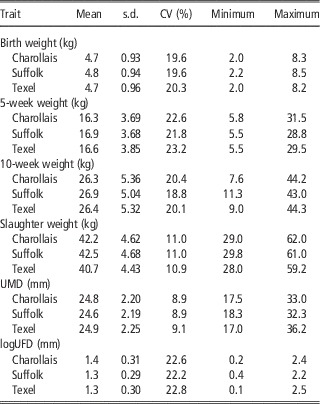
Summary statistics for BWT, 5WT, 10WT, SWT, UMD and logUFD are provided in Table 1 relative to sire breed. As reported previously (Márquez et al., Reference Márquez, Haresign, Davies, Emmans, Roehe, Bünger, Simm and Lewis2012 and Reference Márquez, Haresign, Davies, Roehe, Bünger, Simm and Lewis2013), weights and ultrasound measures differed with respect to sire breed, although changes in means were generally proportional to changes in s.d. (similar CV across breeds).
Summary statistics for birth, 5 week, 10 week and slaughter weights, and for ultrasonic muscle (UMD) and log transformed fat depths (logUFD) by sire breed

Within farm
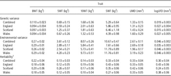
When the data were separated by farm, likelihood ratio tests indicated the presence of heterogeneity in the environmental variance for all traits (P<0.01). However, the estimates of total variance and heritability were similar for the combined data, and for within each subset of farm data (Table 2).
Estimates of genetic and environmental variance and heritability for growth and slaughter traits in sheep. Combined model includes all data, and country subsets includes data only from farm in that country

BWT=birth weight; 5WT=5-week weight; 10WT=10-week weight; SWT=slaughter weight; UMD=ultrasonic muscle depth; logUFD=log ultrasonic fat depth.
1 Heritabilities are without units.
Rank correlations between lamb EBV with the full data and farm subsets ranged from: 0.77 to 0.81 for BWT; 0.55 to 0.93 for 5WT; 0.57 to 0.74 for 10WT; 0.71 to 0.82 for SWT; 0.70 to 0.83 for UMD and 0.76 to 0.95 for logUFD. The rank correlations estimated within a particular farm were not consistently higher or lower than those in the other farms, nor were there clear patterns among correlations within farms. The rank correlations among lamb EBV were higher than those among sire EBV, reflecting the fewer numbers of sires than lambs on individual farms (results not shown).
Across farm
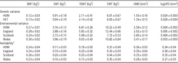
Allowing for heterogeneous environmental variances among farms (Model 2) provided a better fit to the data for all traits (P<0.01). However, when comparing the genetic variances and heritabilities obtained from models with heterogeneous v. homogenous variance structures, they were within the standard error for most traits (except SWT and UMD) (Table 3).
Genetic and environmental variances and heritabilities for homogeneous and heterogeneous variance models for growth and slaughter traits

BWT=birth weight; 5WT=5-week weight; 10WT=10-week weight; SWT=slaughter weight; UMD=ultrasonic muscle depth; logUFD=log ultrasonic fat depth; HOM=homogeneous variances model; HET=heterogeneous variances model.
1 Heritabilities are without units.
Rank correlations between EBV obtained from the homogenous and heterogeneous variance models were 0.99 for all weight traits (both animals and sires), and 0.88 and 0.84 for UMD and logUFD, respectively, among sires. These results indicate that re-ranking only would be observed for ultrasonic traits, although they would not be substantial. The across farm estimates of heritabilities were similar to the within-farm heritabilities of Model 1.
Genotype by environment interaction
For all traits, including a random F×S interaction in the model resulted in a better fit (P<0.001, except P=0.02 for SWT). Heritabilities were similar to those estimated in Models 1 and 2. The proportion of the F×S variance to total variance was small for weight traits, but more pronounced for ultrasonic measures (Table 4). Standardizing traits to a common within-farm variance did not have an effect on variance components or rankings (results not shown).
Variance components estimates for the genetics by environment interaction models for growth and slaughter traits

BWT=birth weight; 5WT=5-week weight; 10WT=10-week weight; SWT=slaughter weight; UMD=ultrasonic muscle depth; logUFD=log ultrasonic fat depth; F×S=sire by farm interaction; G×E=genetics by environment interaction.
1 Heritability and G×E are without units.
2 G×E defined as F×S variance as a proportion of total variance.
Connectedness
Among farm locations, connectedness correlations were between 0.61 and 0.67. Between the high and low index category within a breed, these correlations ranged from 0.44 for the Suffolk to 0.53 for the Charollais. Values between breeds were only slightly lower (0.40). Correlations of 0.10 and above were shown to be indicative of strong connectedness (Kuehn et al., Reference Kuehn, Notter, Nieuwhof and Lewis2008). Although there were only 8 sires shared between Wales and Scotland, 14 between Wales and England, and 13 between Scotland and England, the rotation of rams among farms generated the well-connected design intended.
Discussion
Variance heterogeneity
Heteroscedasticity was present in this population, especially for ultrasonic traits. In the combined data, the additive genetic variance was similar to that estimated within farms (Model 1). These estimates changed little when fitting Model 2. Such was the case even when a homogeneous farm variance was assumed.
For both weight and ultrasound traits, accounting for heterogeneous variances improved model fit. However, for the weight traits, rank correlations between EBV obtained with homogenous and heterogeneous variances were near one. This suggested that any consequences of heteroscedasticity were not pronounced for weight traits, in agreement with previous results (Canavesi et al., Reference Canavesi, Schaeffer, Burnside, Jansen and Rozzi1995). Sire re-ranking was more evident for UMD and logUFD, suggesting heteroscedasticity would have a greater effect on the genetic evaluation of ultrasound traits.
Ignoring heterogeneous variances in genetic evaluation has risks. As observed in this study, animals may be incorrectly ranked resulting in lower selection response. Accuracies of EBV may also be affected. By fitting a heterogeneous variance model, EBV would be scaled, lessening the impact of inaccuracies in the estimation (Gianola, Reference Gianola1986). Given the presence of heterogeneous variances, several livestock breeds have developed genetic evaluation models that account for heteroscedasticity (Wiggans and VanRaden, Reference Wiggans and VanRaden1991; Nakaoka et al., Reference Nakaoka, Narita, Ibi, Sasae, Miyake, Yamada and Sasaki2007).
An effective way to mediate bias in EBV owing to heterogeneous variances would be to test progeny in different environments. In progeny testing of dairy cattle, ranking of bulls was not greatly affected by heteroscedasticity when their daughters were randomly distributed among farms with high and low variances (Winkelman and Schaeffer, Reference Winkelman and Schaeffer1988). Sire referencing schemes, such as those from which the rams used in this study were drawn, provide another way of distributing genetics of sires to many flocks. It has been reported that assumptions of homogeneity may not lead to substantial decreases in selection response when heritabilities are higher in more variable populations (Garrick and Van Vleck, Reference Garrick and Van Vleck1987). No such pattern was found in these data.
Evidence for heterogeneity of variances within individual sheep breeds has been reported. SanCristobal-Gaudy et al. (Reference SanCristobal-Gaudy, Bodin, Elsen and Chevalet2001) found that selecting for increased litter size led to increases in variability of the trait, and that using a heterogeneous variance model resulted in increased selection response. In a study comparing different breeds, Tosh and Kemp (Reference Tosh and Kemp1994) found variable estimates of heritability for weights up to 100 days in three breeds (Hampshire, Polled Dorset and Romanov). They also report heterogeneous breed variances, and suggested accounting for breed specific variance estimates may be necessary when comparing different breeds in an across-breeds genetic evaluation.
Genetics by environment interactions
The ratio of F×S to total variance was shown to be indicative of the presence and influence of G×E within a population (Dickerson, Reference Dickerson1962; Meyer, Reference Meyer1987). For weight traits, F×S explained ~1% of the total variation. For ultrasonic traits, this percentage was greater (10 to 13%), indicating that G×E has a larger influence on body composition traits. For weight traits, our results were similar to Maniatis and Pollott (Reference Maniatis and Pollott2002), also in sheep; however, they reported a lower proportion of variance owing to F×S in ultrasonic traits than in the current study.
In our case, including the F×S effect in the analyses decreased estimates of heritability. Such was also the case for Maniatis and Pollott (Reference Maniatis and Pollott2002). Here, as in their study, ignoring F×S may have inflated estimates of additive genetic variance. They hypothesized that some of the additive genetic variance was being partitioned into the F×S variance component, yielding downwardly biased heritabilities. Shrunk additive genetic variances were also found by Hagger (Reference Hagger1998) for ADG in sheep when fitting an F×S effect. Therefore, levels of G×E in production traits appear to be low but real in sheep populations.
Misztal (Reference Misztal1990) suggested that an explanation for a significant F×S interaction was poor representation of sires across flocks, where genetic evaluations were more severely regressed. In our study, sires were well represented across flocks, with a proportion of sires having progeny in two of the three farms. The connectedness among farms was also strong. Another reason for the F×S interaction may be preferential treatment of some half-sib groups (Meyer, Reference Meyer1987). However, given the design of this experiment, with management intentionally standardized across farms, such would not be anticipated.
Ultrasonic traits had greater indication of heteroscedasticity than weight traits, and also had a higher proportion of variation explained by the F×S interaction. Dickerson (Reference Dickerson1962) and Canavesi et al. (Reference Canavesi, Schaeffer, Burnside, Jansen and Rozzi1995) found that F×S interaction may be caused by, or at least inflated by, heterogeneous variances. When variances were standardized across farms, the variance component estimates, and the proportion of F×S interaction variance to total variance, did not change. Notter et al. (Reference Notter, Tier and Meyer1992) and Maniatis and Pollott (Reference Maniatis and Pollott2002) reported similar results.
Effects on genetic evaluation
Weight at slaughter reflects an animal’s growth to a certain end point, such as a target level of fatness. As such, it is a combination of the bone, fat, lean and other tissues deposited in an animal as it grows. Evidence of heterogeneity and G×E was not observed in SWT, or in earlier weights, but it was in ultrasonic traits. Ultrasonic measures were shown to be indicative of fat and lean tissue deposition in an animal (Emenheiser et al., Reference Emenheiser, Greiner, Lewis and Notter2010), and therefore can be thought of as components of SWT. Perhaps when considering the components rather than the culmination of growth, heterogeneity and G×E become more apparent. Our findings indicate that accounting for heterogeneity and G×E in genetic evaluation of ultrasonic measures, at least in progeny of terminal sires, will reduce such bias.
In selection regimes, where animals were often reared in environments that differed, ignoring G×E when estimating variance components in genetic evaluation led to reductions in selection response (Garrick and Van Vleck, Reference Garrick and Van Vleck1987; Mulder and Bijma, Reference Mulder and Bijma2006). Mulder and Bijma (Reference Mulder and Bijma2005) found that progeny testing schemes were more robust to G×E than sib-testing schemes: when including information on progeny, in the presence of any G×E, the rate of genetic change was greater. The current data were derived from a progeny testing scheme. It was therefore anticipated that it would have less of an impact of G×E than otherwise.
In the presence of G×E, the breeding objective of selection programmes in different environments may differ. The construction of selection tools may also differ because genetic (co)variances between traits may vary across environments. With the presence of G×E, a way to optimize selection programmes would be to have an overall breeding goal yet test progeny in more than one environment, as was the case in the current study.
Clearly the consequences of heteroscedasticity or G×E on genetic evaluation programmes must be carefully considered before being incorporated into genetic evaluation. The limited extent of environmental heteroscedasticity observed in this study may justify it being ignored even for ultrasonic traits, as re-ranking of sires was trivial. Accounting for any G×E in the genetic evaluation of ultrasonic traits may be more important: the F×S random component explained at least 10% of the variation in these traits. Still, to robustly estimate the F×S effect, the number of offspring per sire needs to be large enough and connectedness among their offspring needs to be sufficient. Such was the case in this study but may not be so in industry breeding schemes.
Even where heteroscedasticity or G×E may be important, incorporating them into genetic evaluation schemes could be complicated. First, environments must be delineated. In the current study this was straightforward; by its design, lambs were reared in three distinct locations within the United Kingdom. However, in genetic evaluation schemes, environments may be less easily distinguished, may overlap and may vary gradually across geographic regions and climates. Furthermore, environmental conditions would not be static over time, even on individual farms.
When deciding whether to incorporate G×E or heterogeneous variances into genetic evaluation, the efficacy of running such evaluations also deserves consideration. When fitting models with more random effects, solutions may be more difficult to obtain. Furthermore, the amount of data in current routine genetic evaluations would be large, with computational time a constraint. Therefore, the costs of accounting for heteroscedasticity and G×E in routine, particularly multivariate, genetic evaluations need to be considered.
Conclusions
The aim of genetic evaluation programmes is to assist livestock industries achieve defined breeding goals. The presence of environmental heterogeneity or G×E may hinder progress towards these goals. However, before incorporating such factors into routine genetic evaluations, their extent and consequence on reaching breeding goals need to be carefully evaluated. In the present study, incorporating such comprehensive statistical models for weight traits was not warranted.
Acknowledgements
The authors would like to acknowledge the Meat and Livestock Commission (now English Lamb and Beef Executive (EBLEX), Quality Meats Scotland (QMS), and Hybu Cig Cymru – Meat Promotion Wales (HCC); the UK Department of Environment, Food and Rural Affairs, The British Charollais Sheep Society (Norfolk, UK), the Suffolk Sheep Society (Ballymena, UK) and the British Texel Sheep Society (Kenilworth, UK) for funding of this study. The authors would also like to thank the technical staff at Aberystwyth University, ADAS Rosemaund and the Scottish Agricultural College (now Scotland’s Rural College) for their support of the experimental programme, and E. Stephens for technical editing. The authors acknowledge Advanced Research Computing at Virginia Tech for providing computational resources and technical support that have contributed to the results reported within this paper (http://www.arc.vt.edu).