



1. Introduction
Interest in the friction drag reduction (DR) of a turbulent boundary layer (TBL) has been constantly increasing in the past few decades due to its potential benefits in numerous engineering applications. Skin friction drag is closely connected to quasistreamwise vortices (QSVs). These structures take place largely in the buffer layer, which is immediately above the large wall shear stress (WSS) sublayer (Kravchenko, Choi & Moin Reference Kravchenko, Choi and Moin1993; Orlandi & Jiménez Reference Orlandi and Jiménez1994). The dynamics of these QSVs is directly responsible for the generation of Reynolds shear stress and hence viscous drag. The well-known events, i.e. sweeps and ejections, streaky structures, are all associated with the QSVs (e.g. Kim Reference Kim1983; Hussain Reference Hussain1986). For example, the low-speed streaks result from the ejection process on the upwash side of the QSVs, whilst the high-speed streaks are formed on the downwash side (Kline et al. Reference Kline, Reynolds, Schraub and Runstadler1967). The latter contributes to large skin friction events (Jeong et al. Reference Jeong, Hussain, Schoppa and Kim1997). The streaks are unstable to the normal mode instability (Hamilton, Kim & Waleffe Reference Hamilton, Kim and Waleffe1995) and even more so to the non-normal mode instability (Schoppa & Hussain Reference Schoppa and Hussain2002), giving rise to the streamwise-dependent disturbance and thus the generation of the new QSVs. The inflectional instability is associated with the lifted flows, which accounts for the occurrence of bursts, the major source of turbulence production (Kline et al. Reference Kline, Reynolds, Schraub and Runstadler1967).
The TBL control techniques can be passive or active. Passive techniques, involving no energy input, include riblets (e.g. Walsh Reference Walsh1983; Choi, Moin & Kim Reference Choi, Moin and Kim1993), miniature vortex generators (Zhang et al. Reference Zhang, Luo, Wei and Zhou2023), compliant (e.g. Lee, Fisher & Schwarz Reference Lee, Fisher and Schwarz1993; Choi et al. Reference Choi, Yang, Clayton, Glover, Atlar, Semenov and Kulik1997; Fukagata et al. Reference Fukagata, Kern, Chatelain, Koumoutsakos and Kasagi2008) and superhydrophobic surfaces (e.g. Daniello, Waterhouse & Rothstein Reference Daniello, Waterhouse and Rothstein2009; Martell, Perot & Rothstein Reference Martell, Perot and Rothstein2009; Alamé & Mahesh Reference Alamé and Mahesh2019), etc. These techniques are characterized by permanent fixtures, unable to adapt to varying working conditions. For example, riblets and compliant surfaces suffer from less-efficient DR when flow conditions (e.g. Reynolds number) change, while the performance of superhydrophobic surfaces deteriorates easily in practical environments (Checco et al. Reference Checco, Ocko, Rahman, Black, Tasinkevych, Giacomello and Dietrich2014; Rastegari & Akhavan Reference Rastegari and Akhavan2018). In contrast, active control has the potential to achieve more flexible and drastic flow modifications. Naturally, many active methods have been proposed and investigated with success to different degrees, such as wall oscillation, wall deformation, introducing large-scale streamwise vortices (LSSVs) and blowing or suction, etc. The in-plane wall oscillation is extensively investigated both numerically (e.g. Jung, Mangiavacchi & Akhavan Reference Jung, Mangiavacchi and Akhavan1992; Quadrio & Ricco Reference Quadrio and Ricco2004; Quadrio, Ricco & Viotti Reference Quadrio, Ricco and Viotti2009; Skote Reference Skote2011) and experimentally (e.g. Choi & Clayton Reference Choi and Clayton2001; Di Cicca et al. Reference Di Cicca, Iuso, Spazzini and Onorato2002). This technique may achieve a DR of approximately 40 % (Quadrio Reference Quadrio2011). The wall-normal deformation is another technique. A standing-wave-like wall deformation alone does not result in any significant DR (Mito & Kasagi Reference Mito and Kasagi1998). However, as demonstrated by Endo, Kasagi & Suzuki ’s (Reference Endo, Kasagi and Suzuki2000) and Kang & Choi’s (Reference Kang and Choi2000) direct numerical simulation (DNS) in a turbulent channel flow, this technique may achieve a DR of 10 %–17 % when combined with a feedback control. The wall-normal deformation may also form a spanwise travelling wave, and the experimental (Itoh et al. Reference Itoh, Tamano, Yokota and Taniguchi2006; Li et al. Reference Li, Roggenkamp, Hecken, Jessen, Klaas and Schröder2018) and numerical (Tomiyama & Fukagata Reference Tomiyama and Fukagata2013) studies of this technique demonstrated a DR of 4 %–13 % in TBLs or turbulent channel flow. The streamwise travelling-wave-like wall deformation seems more effective based on the DNS data, achieving a DR of 69 % with a net energy saving of 65 % (Nakanishi, Mamori & Fukagata Reference Nakanishi, Mamori and Fukagata2012) at a low Reynolds number based on u τ (Re τ = 180). This DR technique is, however, less effective when Re τ increases say beyond 1500 based on the scaling analysis by Nabae, Kawai & Fukagata (Reference Nabae, Kawai and Fukagata2020). One drawback associated with the wall deformation or oscillating motion is the difficulty in implementing such techniques in engineering. Introducing artificially LSSVs is another effective method to achieve DR, as demonstrated numerically by Schoppa & Hussain (Reference Schoppa and Hussain1998) and experimentally by Iuso et al. (Reference Iuso, Di Cicca, Onorato, Spazzini and Malvano2003) at a low Reynolds number. Using externally generated LSSVs, Canton et al. (Reference Canton, Örlü, Chin, Hutchins, Monty and Schlatter2016a ,Reference Canton, Örlü, Chin and Schlatter b ) achieved numerically in a turbulent channel flow a DR of 18 % at Re τ = 180 but no DR once Re τ was raised to 550. In their DNS studies, Yao et al. (Reference Yao, Chen, Thomas and Hussain2017, Reference Yao, Chen and Hussain2018) chose correctly the height of an externally generated wall jet and obtained a DR of 12 % at Re τ = 550. Wong et al. (Reference Wong, Zhou, Li and Li2015), Corke & Thomas (Reference Corke and Thomas2018), Thomas et al. (Reference Thomas, Corke, Duong, Midya and Yates2019), Duong, Corke & Thomas (Reference Duong, Corke and Thomas2021), Cheng et al. (Reference Cheng, Wong, Hussain, Schröder and Zhou2021b ) and Wei & Zhou (Reference Wei and Zhou2024, Reference Wei and Zhou2025) developed experimentally plasma actuators for the generation of the LSSVs, achieving substantial DRs, up to 78 %, in TBLs.
Blowing and suction have also been rather extensively studied both experimentally and numerically for the DR of TBLs. It is now well established that steady blowing may reduce the skin friction, accompanied by a rapid decrease in turbulence intensity near the wall but an increase farther away from the wall, which is related to the up-lifted streamwise vortices (Park & Choi Reference Park and Choi1999; Kametani & Fukagata Reference Kametani and Fukagata2011). On the other hand, suction does the opposite (Park & Choi Reference Park and Choi1999; Kim, Kim & Sung Reference Kim, Kim and Sung2003). However, the skin friction farther downstream of the control area shows the opposite, i.e. an increase in the blowing case and a decrease in the suction case, which is ascribed to the flow destabilization and stabilization by blowing and suction, respectively, as observed by Antonia, Zhu & Sokolov (Reference Antonia, Zhu and Sokolov1995) in a TBL control experiment when suction was done through a short porous spanwise wall strip. In fact, given an adequately high suction rate, the pseudorelaminarization took place downstream of suction, leading to a DR of 50 %. Periodic blowing experimentally through a spanwise slot may result in a temporal relaminarization within 40 wall units downstream of the slot, achieving a local DR of 45 % but producing a drag increase of 200 % farther downstream (Tardu Reference Tardu2001). The periodic blowing through one array of streamwise slits may lead to a maximum DR of 70 % in the experiment, even with a net energy saving of 2.2 % (Cheng et al. Reference Cheng, Qiao, Zhang, Quadrio and Zhou2021a ).
Attention has also been given to TBL control via wall normal synthetic jets in the experiment, which can be generated through circular or rectangle orifices. Circular synthetic jets can achieve a local DR of 12 %–30 % downstream of the actuator (Spinosa & Zhong Reference Spinosa and Zhong2017; Lu et al. Reference Lu, Li, Gao, Cao, Bai and Zheng2020). Rathnasingham & Breuer (Reference Rathnasingham and Breuer2003) used three synthetic jets through streamwise slits to manipulate a TBL. The slits of 160 wall units (l
 $_{v}$
) in length and 10 l
 $_{v}$
in width were spanwise-separated by 40 l
 $_{v}$
, where l
 $_{v}$
is the wall unit. They reported a local maximum DR of 7 % downstream of the synthetic jets. Ye et al. (Reference Ye, Jiang, Zhang, Zou and Zheng2019) used one array of synthetic jets through longer (400 l
 $_{v}$
) and wider (26.7 l
 $_{v}$
) slits, where the spanwise separation between slits was 560 l
 $_{v}$
. The local DR reached 30 %. Yu et al. (Reference Yu, Fan, Noack and Zhou2022) developed one array of six synthetic jets through smaller scale longitudinal slits, with 150 l
 $_{v}$
in length, 6.7 l
 $_{v}$
in width and a spanwise spacing of 20 l
 $_{v}$
. They measured a maximum local DR of 48 % downstream of the slits.
Active control often involves more than one control parameter. Conventional open-loop control searches for optimal performance by manually adjusting individual control parameters which is time-consuming and inefficient. Closed-loop control may adjust the control parameters dynamically based on the feedback or feedforward information on the control target (Qiao, Zhou & Wu Reference Qiao, Zhou and Wu2017). The proportional integral derivative and opposition controllers have demonstrated their effectiveness and efficiency in reducing skin friction of the TBL (Choi, Moin & Kim Reference Choi, Moin and Kim1994; Abbassi et al. Reference Abbassi, Baars, Hutchins and Marusic2017; Qiao et al. Reference Qiao, Zhou and Wu2017; Qiao, Wu & Zhou Reference Qiao, Wu and Zhou2018). However, the closed-loop control may in general optimize only up to two or three control parameters (Wu, Wong & Zhou Reference Wu, Wong and Zhou2018; Fan, Zhou & Noack Reference Fan, Zhou and Noack2020b ). A large number of control parameters or a large opportunity space is bound to contain more desirable solutions, and the associated optimal or near optimal solutions may exceed greatly that offered by the opportunity space of two or three control parameters. However, it is a challenge to find optimal control laws when many control parameters are involved.
Machine learning or artificial intelligence (AI) control provides a powerful vehicle for optimizing active flow control. Various techniques based on different algorithms have been developed, including linear genetic programming (e.g. Gautier et al. Reference Gautier, Aider, Duriez, Noack, Segond and Abel2015; Li et al. Reference Li, Noack, Cordier, Borée and Harambat2017), genetic algorithm (GA) (e.g. Minelli et al. Reference Minelli, Dong, Noack and Krajnović2020; Qiao et al. Reference Qiao, Minelli, Noack, Krajnović and Chernoray2021; Yu et al. Reference Yu, Fan, Noack and Zhou2022), reinforcement learning (e.g. Rabault et al. Reference Rabault, Kuchta, Jensen, Réglade and Cerardi2019; Lai et al. Reference Lai, Wang, Zhang and Xu2021; Paris, Beneddine & Dandois Reference Paris, Beneddine and Dandois2021), explorative gradient method (EGM) (e.g. Fan et al. Reference Fan, Zhang, Zhou and Noack2020a ; Li et al. Reference Li, Cui, Jia, Li, Yang, Morzyński and Noack2022) and ant colony optimization (Zhang et al. Reference Zhang, Fan and Zhou2023a ). Zhou et al. (Reference Zhou, Fan, Zhang, Li and Noack2020) provided an excellent demonstration on how AI can find the optimum control strategies and provide new insight into the flow physics. They developed an AI control system based on linear genetic programming for enhancing a turbulent jet mixing using six independently operated distributed minijets as actuators, involving the optimization of 18 independent parameters. Their analysis of the proximity map or all the control strategies identified in the learning process unveiled four distinct flow structures, i.e. three classical forcings (axisymmetric forcing, helical forcing and flapping) and a highly complicated forcing never reported before. The new forcing is characterized by, inter alia, both swirling around an oscillating axis and three-dimensional (3-D) flapping, much more effective in enhancing mixing than those classical ones.
There is a scarcity of research on the machine-learning-based control of TBL due to a few challenges related to this highly complex flow, including how to capture reliably the friction force and how to manipulate the flow. The latter involves the difficulties in the development of actuator and controller. Yu et al. (Reference Yu, Fan, Noack and Zhou2022) developed a GA-based evolutionary control system to manipulate a TBL. A maximum local DR of 48 % was obtained 33 l
 $_{v}$
downstream of the synthetic jets. This very first attempt suffers from several limitations. Firstly, they used only six independently operated synthetic jets through longitudinal slits, covering an actuation width of only 100 l
 $_{v}$
, corresponding to the average separation between low-speed streaky structures (Kline et al. Reference Kline, Reynolds, Schraub and Runstadler1967). Secondly, their investigation involved only six independent control variables, i.e. the initial phases of the synthetic jets. The search space is relatively small. Thirdly, the cost function consisted of local WSS from only two wall wires, implying locally targeted DR and giving no information on the spanwise averaged DR. Fourthly, they reported only the maximum DR and did not analyse the large amount of data generated during the learning process, thus missing possibly valuable information associated with the data. For example, how was the optimal solution found? Was there any alternative optimal solution? Finally, little information was given on how the flow structure altered under control and what the DR mechanisms were.
The purpose of this experimental work is to address the aforementioned issues. The manuscript is organized as follows: §§ 2 and 3 describe the experimental set-up and synthetic jet-induced flow, respectively. The control system and how it works are presented in § 4. The data-driven optimization process and the performances of representative optimized control laws or individuals are given in § 5. The modified flow structures and the mechanisms for DR are discussed in § 6. This work is concluded in § 7.
2. Experimental details
2.1. Generation of fully developed TBL
Experiments were carried out in a closed-loop wind tunnel, with a horizontal test section of 5.6 m in length, 0.8 m in width and 1.0 m in height, at The Center for Turbulence Control, Harbin Institute of Technology (Shenzhen). The rig to generate zero-pressure-gradient TBL is the same as Cheng et al. (Reference Cheng, Qiao, Zhang, Quadrio and Zhou2021a
,Reference Cheng, Wong, Hussain, Schröder and Zhou
b
), thus not repeated here. Measurements were conducted at a free stream velocity U
∞
= 2.4 ms−1, and the corresponding free stream longitudinal turbulence level was 0.4 %. Table 1 lists the characteristic parameters of the uncontrolled TBL at the test position, 3.2 m downstream of the leading edge of the plate (figure 1), including the TBL thickness δ
99, momentum thickness θ, displacement thickness δ
1, shape factor H
12 = δ
1
/θ, friction velocity
 $u_{\tau}$
(
 $\equiv \sqrt{\overline{{\tau }_{{w}}}/{\rho }}$
, where τ
w
is the local WSS, ρ is the density of air and the overbar denotes time-averaging),
 $l_v$
= ν/u
τ
(ν is the kinetic viscosity of air), time scale t
 $_{v}$
=
 $l_v/u_{\tau}$
, Reynolds number
 $\mathit{R}\mathit{e}_{{\theta }}=\mathit{U}_{{\infty }}{\theta }/{\nu }$
,
 $\mathit{R}\mathit{e}_{{{\delta }_1}}=\mathit{U}_{{\infty }}{\delta }_{1}/{\nu }$
and
 $\mathit{R}\mathit{e}_{\tau }=\mathit{u}_{{\tau }}{\delta }_{99}/{\nu }$
. Unless otherwise stated, the superscript ‘+’ and ‘*’ in this paper denote normalization by the inner and outer scales in the absence of control, respectively. The coordinate system (x, y, z) is defined in figure 1, with its origin at the trailing edge and symmetry point of the synthetic minijet array. The instantaneous velocities along the x, y and z directions are denoted by
 $\mathit{U}=\overline{\mathit{U}}+\mathit{u}$
,
 $\mathit{V}=\overline{\mathit{V}}+\mathit{v}$
and
 $\mathit{W}=\overline{\mathit{W}}+\mathit{w}$
, respectively, where u, v and w are the fluctuating components.
Characteristic parameters of the uncontrolled TBL.

Schematic of the experimental set-up, including the actuator, its installation, the measurement and the workflow of data-driven optimization (not to scale; units in millimetres).

Figure 1. Long description
The diagram illustrates an experimental setup for turbulent boundary layer control. It features an actuator with a PZT membrane and synthetic jets array, installed in a wind tunnel with dimensions labeled in millimeters. The setup includes a tripping device, smoke wire visualization, and a moveable hot-wire. Sensors, including nine wall wires, provide measurement signals to a GA control platform connected to a computer and dSpace system. The workflow involves generating sinewave signals to control the actuator, with feedback loops for optimization. The overall structure shows the interaction between the actuator, sensors, and control platform to achieve drag reduction in turbulent boundary layers.
2.2. Actuator and control platform
The actuator consists of one array of 11 synthetic jets through longitudinal slits, fabricated in-house and spanwise-arranged uniformly. The innovativeness of this actuator lies in the miniature size of the synthetic jets and furthermore each jet can be independently operated. Both features are crucially important for this investigation. Firstly, each slit has a width of 7l
 $_{v}$
and a longitudinal length of 160l
 $_{v}$
, and the spanwise centre-to-centre separation between adjacent slits is 20l
 $_{v}$
, comparable to those (3l
 $_{v}$
, 133l
 $_{v}$
and 20l
 $_{v}$
) used by Cheng et al. (Reference Cheng, Qiao, Zhang, Quadrio and Zhou2021a). These dimensions are in the same order of magnitude as those of predominant coherent structures in the TBL (Jacobson & Reynolds Reference Jacobson and Reynolds1998). For example, the QSVs feature with a length of approximately 200l
 $v$
(Smith Reference Smith1984) and the low-speed streaks are on average approximately 60
 $l_v$
in width and 1000
 $l_v$
in length, with a spanwise separation of 100
 $l_v$
(Kline et al. Reference Kline, Reynolds, Schraub and Runstadler1967; Smith Reference Smith1984). Secondly, as demonstrated by Zhou et al. (Reference Zhou, Fan, Zhang, Li and Noack2020), AI may have great advantages over conventional control techniques only when involving many control variables, in general exceeding three, and its deployment may find new control strategies and mechanisms. Cheng et al.’s (Reference Cheng, Qiao, Zhang, Quadrio and Zhou2021a) minijets were synchronized since it would be extremely difficult, if not impossible, to make their minijets independently operated due to the very small spanwise centre-to-centre separation between adjacent slits and the bulky size of electromagnetic valves involved. However, the present innovative actuator overcomes this difficulty, each synthetic minijet being independently operated, thus with up to 33 independent control variables.
The synthetic minijet is generated by a vibrating piezoelectric (PZT) membrane of 30 mm × 20 mm × 0.2 mm (length × width × thickness). As shown in figure 1, this membrane is mounted vertically, with both ends fix-supported, in a chamber made of an aluminium alloy base. The separation between the membrane and the base wall is 0.7 mm, larger than the maximum oscillation amplitude of the membrane to avoid a clash. The thickness of the wall between two adjacent chambers is 1 mm. It has been confirmed that there is no interaction in terms of vibrations between two adjacent units. Every membrane is monitored in its capacitance, approximately 1 μF, during experiments to ensure its good working order. Driven by a sinusoidal signal, the oscillating membrane creates a synthetic jet through a longitudinal slit of 1 mm in width and 24 mm in length. The entire synthetic jet array occupies an area of 32 mm (spanwise) × 24 mm (streamwise) or 200 l
 $_{v}$
× 160
 $l_v$
, and the spanwise separation of adjacent slits is 3 mm or 20 l
 $_{v}$
. A synthetic jet S
i
is driven by an independent sinusoidal signal V
t,i
= V
0,i
sin (2πf
i
t +
 ${\phi }$
i
), i = 1, 2, …, 11, generated from the dSPACE control system (t is time). The peak voltage V
0,i
and frequency f
i
can be any value in 0∼30 V and 200∼600 Hz, respectively. Beyond this frequency range, the PZT membrane may vibrate irregularly. Here
 ${\phi }_{\mathit{i}}$
is the initial phase, where
 ${\phi }_{1}$
is set to zero to avoid reduplicated actuation strategies.
A real-time control platform dSPACE is deployed to process the input signals and output control signals based on the user-defined control logic. The outputs from the 16-bit digital-to-analogue converter of the platform are amplified by a dual channel piezo driver amplifier (Trek PZD 700) to drive the PZT membranes. All input and output signals are recorded synchronously at a sampling frequency of 5 kHz.
2.3. Flow measurements
A total of nine fixed wall wires and one movable hot-wire (Dantec 55P15) are used to measure the local WSS and the velocity profile in the TBL, respectively. The sensing element of each wire, made of tungsten, was 5 μm or 0.033
 $l_v$
in diameter and 1.2 mm or 8 l
 $_{v}$
in length. The overheat ratio was set as 1.5 for all wires. The wires were operated on constant-temperature anemometers (Dantec Streamline). The signal from the wire was low-pass filtered at a cutoff frequency of 3 kHz and then sampled at 6 kHz using a 16-bit analogue-to-digital converter. The movable hot-wire was mounted on a 3-D traversing mechanism, with a spatial resolution of 3.125 μm in all three directions. The hot-wire is calibrated with a Pitot tube connected to a micromanometer (FCO510, with a resolution of 0.001 Pa). The WSS can be estimated by the slope of
 $\overline{\mathit{U}}$
profile in the viscous sublayer measured using the movable hot-wire, following, e.g. Hutchins & Choi (Reference Hutchins and Choi2002). The profile consists of 26 points along the y direction with an increment of 0.025 mm, as illustrated in figure 2. The duration of each hot-wire signal was recorded for 40 s. Evidently, the data are well fitted to a linear curve, except for a couple of points near the wall deviating from the linear curve due to the wall effect (Hutchins & Choi Reference Hutchins and Choi2002). As such, we may determine the wall position, and the distance y of the measurement point from the wall. Following Qiao, Xu & Zhou (Reference Qiao, Xu and Zhou2019), we used a total station theodolite to measure the position y
0 of the valid measurement point nearest to the wall. The maximum difference between two different estimates in y
0 is no more than 3 %. Then, the time-averaged WSS
 $\overline{{\tau }_{{w}}}$
can be calculated from
 $\overline{{\tau }_{{w}}}={\mu }({\mathrm{d}\overline{\mathit{U}}}/{\mathrm{d}\mathit{y}})$
, and five repeated measurements indicate an uncertainty of no more than 1.8 %.
Comparison in the time-averaged streamwise velocity between the wall wire (
 $\blacksquare$
) and traversing hot-wire (□) measurements.

Figure 2. Long description
A line graph comparing time-averaged streamwise velocity between wall-wire and traversing hot-wire measurements. The x-axis represents distance in millimeters, ranging from 0 to 1. The y-axis represents velocity in meters per second, ranging from 0 to 1. The red line represents wall-wire measured data, while the black line represents movable hot-wire measured data. The graph highlights a linear region between approximately 0.3 and 0.7 millimeters on the x-axis. The wall-wire measured data point at approximately 0.4 millimeters on the x-axis and 0.4 meters per second on the y-axis is marked with a red square. All values are approximated.
Additional, nine wall-wires named W
1 ∼ W
9 were placed at x
+
= 100 (figure 1), downstream of the second through 10th slit, respectively, to measure the local WSS or drag variation. The sensing element and supporting prongs are immersed in the TBL, producing a minimum disturbance to the flow. As in figure 2, the thermal effect of the wall could be felt at y
+
< 3 (Hutchins & Choi Reference Hutchins and Choi2002). Therefore, the distance between wall-wire and the wall was 0.5 mm or 3.3
 $l_v$
. The calibration process for the wires is the same as Qiao et al. (Reference Qiao, Zhou and Wu2017). Because the wall wire was placed in the viscous layer or linear region whose thickness was approximately 0.75 mm, the WSS can also be calculated from
 $\overline{{\tau }_{{w}}}={\mu }({\mathrm{d}\overline{\mathit{U}}}/{\mathrm{d}\mathit{y}})={\mu }({\overline{\mathit{U}_{{w}}}}/{\mathit{y}})$
, where
 $\overline{\mathit{U}_{{w}}}$
and y are the wall-wire-measured velocity, time-averaged over a duration of 40 s, and the wire distance from the wall. The accuracy of this method is slightly lower than the first method based on the slope of
 $\overline{\mathit{U}}$
in viscous layer, and the uncertainty of five repeated measurements is 3 %. This method is only used in the data-driven optimization process to reduce the cost of time. Once an optimal control strategy is identified,
 $\overline{{\tau }_{{w}}}$
will be remeasured using the first method. Subsequent
 $\overline{{\tau }_{{w}}}$
downstream of the actuation is also measured using the first method. The corresponding local time-averaged drag variation
 $\overline{{\delta }_{{{\tau }_{{w}}}}}=[(\overline{{\tau }_{{w}}})_{\textit{on}}-(\overline{{\tau }_{{w}}})_{\textit{off}}]/(\overline{{\tau }_{{w}}})_{\textit{off}}$
, where the subscripts ‘on’ and ‘off’ denote the values with and without control, respectively.
A Dantec particle image velocimetry (PIV) system was deployed to measure the TBL and the actuator-induced flow in different planes. The tracer particles with an average diameter of approximately 1μm were generated from olive oil by a particle generator (TSI 9307-6). A double-pulse laser system with a spherical lens and a cylindrical lens creates a laser sheet of 1 mm thickness. One charge-coupled device (CCD) camera was used to capture the images in the mode of double frames (2560 pixels × 1600 pixels). The image covers an area of 46 mm × 30 mm for measurements in the x–y planes of z
+
= 0 and –70 or an area of 40 mm × 25 mm in the y–z plane of x
+
= –80. A total of 2700 image pairs were captured in each plane at a framing rate of 15 Hz. A low-frequency laser with the trigger frequency f
t
= 15 Hz is unable to capture the full picture of the flow at the various phases of synthetic jets. However, given specific imaging frequencies, i.e. kf
t
+ 1 Hz (k is a positive integer), the CCD camera captures the first pair of images at t = 0 in the first cycle of the synthetic jets, the second and third pairs at
 $\mathit{t}=\mathit{k}({1}/{15})\mathit{T}$
and
 $\mathit{k}({2}/{15})\mathit{T}$
, respectively, where
 $\mathit{T}$
is the period of the synthetic jets. Then we may obtain 15 different phases of the synthetic jets. For instance, take T = 0.002 s, then the 15 Hz laser can only capture three phases of the synthetic jets but may capture 15 phases of the synthetic jets given kf
t
+ 1 = 496 Hz (k = 33). Therefore, in PIV experiments, we used the synthetic jets of 496 Hz instead of 500 Hz. It has been confirmed that mean velocity, vorticity, production and dissipation of turbulent kinetic energy (TKE) all converged to a maximum departure of 1 % once the number of images exceeds 2000 pairs.
The PIV system was also used for smoke-wire flow visualization in the x–z plane of y + = 7 in the TBL, though the double-pulsed laser was replaced by a continuous laser source. The smoke wire made of NiCr alloy with a diameter of 0.05 mm was placed at y + = 5, oriented parallel to the plate and perpendicular to incoming flow. A uniform smoke sheet is produced once the wire is heated by an adequately strong direct electric current. Here U ∞ is chosen to be 1.8 ms−1 to ensure high-quality flow visualization images. The imaging rate was 500 frames (120 mm × 75 mm) per second.
3. Natural TBL and synthetic jets
3.1. The TBL in the absence of control
It is important to ensure the generation of a fully developed TBL at the position where the measurements are conducted. The TBL in our work is fully developed, characterized by zero-pressure gradient. The Reynolds numbers,
 $\mathit{R}\mathit{e}_{{\theta }}$
and
 $\mathit{Re}_{{{\delta }_{1}}}$
, based on the momentum thickness and displacement thickness, respectively, with a shape factor of H
12 = 1.41, which is very close to the reported results. The shape factor H
12 Spalart (Reference Spalart1988) measured is 1.43 at
 $\mathit{R}\mathit{e}_{{\theta }}$
= 1410, and Cheng et al. (Reference Cheng, Qiao, Zhang, Quadrio and Zhou2021a
,Reference Cheng, Wong, Hussain, Schröder and Zhou
b
) found H
12 = 1.41 at
 $\mathit{R}\mathit{e}_{{\theta }}$
= 1450. Pirozzoli & Smits (Reference Pirozzoli and Smits2023) summarized the characteristic properties of the zero-pressure gradient TBL (
 $\mathit{Re}_{{{\delta }_{1}}}$
= 103 ∼ 105) and showed that H
12 gradually decreased from 1.5 to 1.2 with increasing
 $\mathit{Re}_{{{\delta }_{1}}}$
. At
 $\mathit{Re}_{{{\delta }_{1}}}$
= 2000, H
12 is approximately 1.42. The
 $\overline{\mathit{U}^{+}}$
and
 ${\mathit{u}}_{\mathit{rms}}^{+}$
profiles of the baseline TBL collapse well with the published canonical TBL data, as shown in figure 3. Furthermore, these profiles measured at z
+
= 0 and ± 150 also exhibit a good collapse, suggesting a spanwise homogeneity.
Distributions of (a) time-averaged streamwise velocity
 $\overline{\mathit{U}^{+}}$
and (b) r.m.s. value
 ${\mathit{u}}_{\mathit{rms}}^{+}$
at three different spanwise locations (x
+ = 33, z
+ = −150, 0, 150) in the natural TBL.

Figure 3. Long description
The line graph presents two subplots. Subplot (a) displays the distributions of time-averaged streamwise velocity (U+) against the wall-normal coordinate (y+). The data is represented by four different markers: squares for z+ equals 0, triangles for z+ equals negative 150, diamonds for z+ equals 150, and plus signs for Cheng et al. (2021a). A dashed line represents the Spalart (2009) model. The graph shows a logarithmic trend line with the equation U+ equals 2.44 times the natural logarithm of y+ plus 5.1. Subplot (b) shows the distributions of the root mean square (r.m.s.) value of streamwise velocity fluctuations (u+r.m.s+) against the wall-normal coordinate (y+). The data is represented by the same markers as in subplot (a), and a dashed line represents the Spalart (1988) model. The graph shows a peak around y+ equals 10 and a gradual decrease thereafter. All values are approximated.
3.2. Characteristics of synthetic jets
It is important to document the characteristics of the synthetic jets. A single hot-wire is placed parallel to the slit at (x + , y + , z + ) = (–80, 3.3, 0) to measure the exit velocity U jet + at the centre of the middle slit in the absence of incoming flow. Figure 4 illustrates the time histories of U jet + and the input signal V t of the PZT membrane. Note that a second minor peak in V t results from the flow reversal associated with the synthetic jet. The lasting durations of blowing and suction, marked by the dashed and dotted lines, are identical. The peak of blowing is higher than that of suction, as noted by Utturkar et al. (Reference Utturkar, Arik, Seeley and Gursoy2008) and Qayoum et al. (Reference Qayoum, Gupta, Panigrahi and Muralidhar2010), largely due to a difference in the effective cross-sectional area at the jet exit between the two stages. The actuator is characterized via a delay in response time by 0.12 ms as shown in figure 4. Before experiments, the time delays of all synthetic jets were measured and adjusted on the dSPACE control system to ensure that they were identical to each other.
Control and typical velocity signals measured at (x + , y + , z + ) = (–80, 3.3, 0) using a hot-wire. The voltage on PZT membrane is 500 Hz and 40 V.

Figure 4. Long description
The line graph presents data on the relationship between time (t) in seconds on the x-axis and voltage (V) on the y-axis for three different signals: blowing, suction, and control signal. The blowing signal is represented by a red dashed line, the suction signal by a red dotted line, and the control signal by a black solid line. The graph shows periodic oscillations for all three signals, with the control signal leading the blowing and suction signals. The blowing signal reaches a peak voltage of 20 volts, while the suction signal reaches a trough of -20 volts. The control signal oscillates between 20 and -20 volts. A notable feature is the 0.12 millisecond delay between the control signal and the blowing signal. The graph illustrates the dynamics of quasistreamwise vortices (QSVs) and their impact on skin friction drag in a turbulent boundary layer.
4. Data-driven optimization
4.1. Control system
It is a challenge for conventional optimization methods to deal with a problem with a large number of variables where 33 independent parameters (V
0,i
, f
i
, ϕ
i
, i = 1, 2, …, 11) are involved with the 11 spatially distributed synthetic jets. It is the data-driven optimization that provides us with a means to find the optimal or near optimal solution to this problem. Our developed data-driven optimization system is schematically shown in figure 5. The system consists of the control plant (TBL), actuation unit (11 synthetic jets), sensing unit (nine wall wires) and control unit based on GA. The control plant, actuation unit and sensing unit have been discussed in §§ 2.1, 2.2 and 2.3, respectively. The control goal is to minimize the cost function J, defined as
 $\mathit{J}=1+({1}/{9}){\sum }_{\mathit{i}=1}^{9}\overline{{\delta }_{{{\tau }_{{w}}}\mathit{,}\mathit{i}}}$
, where
 $\overline{{\delta }_{{{\tau }_{{w}}}\mathit{,}\mathit{i}}}$
is the time-averaged drag variation measured from the ith wall wire W
i
. Thus, a minimized J corresponds to the maximum spanwise averaged DR at x
+
= 100.
Workflow of data-driven optimization system.

Figure 5. Long description
The diagram illustrates the workflow of a data-driven optimization system designed to reduce friction drag in a turbulent boundary layer. At the top, a control plant is depicted with a turbulent boundary layer, showing the interaction between the flow and the surface. Below the control plant, the diagram splits into two main units: the actuation units and the sensing unit. The actuation units consist of eleven synthetic jets, which are used to manipulate the flow. The sensing unit comprises nine wall wires, which detect changes in the flow. These units are connected to a control unit that employs a genetic algorithm to optimize the system. The arrows indicate the flow of data and control between these components, demonstrating how the system senses, actuates, and optimizes to reduce friction drag.
The present choice of the GA is due to following considerations. First, the wall-wire-measured DR contains errors, which introduces noises in the estimation of the cost function. The GA is robust to such noises, thanks to the repeated crossover and re-evaluation of individual control strategies (e.g. Zhou et al. Reference Zhou, Fan, Zhang, Li and Noack2020). As such, this algorithm is commonly used in experiments targeting the optimization of flow control (e.g. Benard et al. Reference Benard, Pons-Prats, Periaux, Bugeda, Braud, Bonnet and Moreau2016; Debien et al. Reference Debien, von Krbek, Mazellier, Duriez, Cordier, Noack, Abel and Kourta2016; Qiao et al. Reference Qiao, Minelli, Noack, Krajnović and Chernoray2021; Zigunov, Sellappan & Alvi Reference Zigunov, Sellappan and Alvi2021). In contrast, the gradient-based methods heavily rely on the gradient information and are prone to being misled by experimental noises, even falling into local optima (Lou, Sun & Nocedal Reference Lou, Sun and Nocedal2025). Second, the number of sensors presently optimized is limited, only nine, making it difficult to use methods like DRL that require a large number of sensors (Paris et al. Reference Paris, Beneddine and Dandois2021). For instance, Rabault et al. (Reference Rabault, Kuchta, Jensen, Réglade and Cerardi2019) and Tang et al. (Reference Tang, Rabault, Kuhnle, Wang and Wang2020) used 151 and 236 probes, respectively, to control the two-dimensional wake of a cylinder. Finally, an algorithm must possess strong global search capabilities to handle the high nonlinearity of a TBL and a large sample space, involving presently more than 10 parameters. The GA has reached a relatively mature stage of development, and its widely recognized global search capability is particularly prominent when dealing with high-dimensional complex optimization problems (Brunton & Noack Reference Brunton and Noack2015). In our preliminary work, we compared the search performances of EGM (Li et al. Reference Li, Cui, Jia, Li, Yang, Morzyński and Noack2022) and GA. The EGM combines the downhill simplex method for local extremum search and Latin hypercube sampling for global search. Although the EGM algorithm could discover better control strategies than conventional uniform forcing (CUF) and converge faster than GA, its converged result remained inferior to those of GA. Analysis of the search process or landscape reveals that, while the Latin hypercube sampling method exhibits a certain level of global search capabilities, its random search efficiency is excessively low for high-dimensional and complex sample spaces, leading to a premature convergence to local optima. Indeed, the GA may find control strategies that are completely out of our expectation and uncover new physical mechanisms of DR. In their jet-mixing optimization, Zhou et al. (Reference Zhou, Fan, Zhang, Li and Noack2020) demonstrated that linear genetic programming, a GA-based algorithm, progressively identified the well-known jet-mixing mechanisms and eventually converged to a never reported highly effective jet-mixing mechanism. The TBL is a highly complex flow, compared with a turbulent jet. As such, we deployed in the first stage actuators with a search space as large as 33 parameters (synthetic jet frequency, exit momentum and phase). However, we failed to find any good control strategy (to be discussed later). This is because GA cannot get around the curse of dimensionality when dealing with very high-dimensional complex sample spaces; with increasing population sparsity, the algorithm tends to degenerate into a random search (Goldberg Reference Goldberg1989). As such, we choose to optimize the excitation frequency and exit momentum first and then optimize the individual phases of the synthetic jets, thus reducing the search space to a maximum of 11 control parameters.
4.2. Optimization based on GA
The actuation commands are given by V t = [V t,1, V t,2, …, V t,11], where V t,i = V 0,i sin (2πf i t + ϕ i ) is the actuation signal for the ith synthetic jet. Vectors V 0 = [V 0,1, V 0,2, …, V 0,11], f = [f 1, f 2, …, f 11] and ϕ = [ϕ 1, ϕ 2, …, ϕ 11] are considered to be optimized. A GA-based optimization searches for individuals,
 \begin{equation} \boldsymbol{K}=\left(\boldsymbol{V}_{0},\boldsymbol{f},\boldsymbol{\phi }\right) \end{equation}
so that the cost is minimized, and the optimal individuals is
 \begin{equation}\boldsymbol{K}^{\star }=\arg \min _{\boldsymbol{K}} \mathit{J}\left[\boldsymbol{K}\right]\!.\end{equation}
The first generation of GA contains N i = 100 sets of rather randomly chosen control parameters, and each set is also referred to as an individual or control law. In the searching process of the data-driven optimization system (figure 5), every individual is tested for 40 s to estimate the corresponding cost function J i n , where the superscript n denotes the nth generation. There is a 5 s interval from the evaluation of one individual to another to minimize the interference between evaluations. Subsequent generations are produced from the previous one with genetic operations, i.e. elitism, crossover, mutation and replication, which will be discussed in detail later. Again, the evaluation of the individuals in new generation is the same as the previous generation. After the in situ performance evaluations, the individuals in each generation are renumbered in descending order, viz.
 \begin{equation} {J}_{1}^{n}\leqslant {J}_{2}^{n}\leqslant \ldots \leqslant {J}_{N_{i}}^{n} {J}_{1}^{n}\leqslant {J}_{2}^{n}\leqslant \ldots \leqslant {J}_{N_{i}}^{n}. \end{equation}
where the subscript i represents the individual index. The above processes are repeated until the cost functions are converged.
4.3. Choices of GA parameters
The choice of the GA parameters needs to take into account both convergence speed and optimization results. Elitism is a process that passes a given number of top-ranking individuals directly to the next generation, thus guaranteeing that the next generation will not perform worse than the previous one. The individuals of the next generation are selected via a tournament process. A certain number, determined by the tournament size N t , of randomly chosen individuals, compete in a tournament and the winner is selected based on the value of J. Replication copies a statistically selected number of individuals into the next generation. Thus, some well-performing individuals are preserved. Crossover involves two statistically selected individuals from the tournament and generates a new pair of individuals, with part of their parameters swapped. This operation contributes to breeding better individuals by searching the space around well-performing individuals. The mutation operation, where the random parts of the statistically selected individuals are modified, serves to explore potentially new individuals with a smaller J. The parameters of GA in this study are given in table 2. Following Yu et al.’s (Reference Abbassi, Baars, Hutchins and Marusic2021) preliminary work, the choice of the parameters was obtained after numerous trial-and-error tests. The number of top-ranking individuals is chosen to be N e = 3 for elitism operation. The size for tournament is set as N t = 7. The population size N i of each generation is set as 100. There should be a compromise between reduced populations (approximately 50–500) and high mutation rates P m (from 25 % to 50 %) to ensure diversity (Duriez, Brunton & Noack Reference Duriez, Brunton and Noack2017). Therefore, P m is set as 30 %. On the other hand, the crossover rate P c influences the ability to global search and is generally higher than P m (Duriez et al. Reference Duriez, Brunton and Noack2017), thus being made 50 %. Finally, replication ensures the exploration of a given search space during a certain number of generations and its rate P r is set as 20 % since P c + P m + P r = 1.
Key parameters of GA.

Table 2. Long description
The table presents key parameters of a genetic algorithm (GA) with their respective values. It includes six rows and two columns. The first column lists the parameters: Population size, Elitism, Tournament size, Crossover, Mutation, and Replication. The second column provides the corresponding values: Population size is 100, Elitism is 3, Tournament size is 7, Crossover is 50 percent, Mutation is 30 percent, and Replication is 20 percent. The table provides a clear and concise overview of the GA parameters used in the study.
Note that the choice of the GA parameters does have an impact upon the optimization performance. In almost all algorithms, including GA, the hyperparameters may affect the optimization performance. Tuning these parameters is always an important part of data-driven optimization. However, there are many references that document the choice of the parameters, especially for matured algorithms such as GA. The influence of each parameter is quite predictable on the search performance. Therefore, this disadvantage is acceptable as per the good results it may lead to.
4.4. Control landscape
Insight into the control landscape or overall picture and its evolution of control laws may be gained from proximity maps via multidimensional scaling (Cox & Cox Reference Cox and Cox2000). The essence of this scaling is to ensure that the relative distances between the examined control laws or individuals are essentially unchanged after a high-dimensional space is mapped to a two-dimensional space γ i = (γ i,1, γ i,2). This method is employed in a number of investigations (e.g. Duriez et al. Reference Duriez, Brunton and Noack2017; Zhou et al. Reference Zhou, Fan, Zhang, Li and Noack2020), to produce the proximity map of individuals. Its key is to find a feature vector γ i so that
 \begin{equation} \sum\limits_{i=1}^{N_{i}\times n} \sum\limits_{j=1}^{N_{i}\times n}(|| \boldsymbol{\gamma }_{i}-\boldsymbol{\gamma }_{\!j}|| -D_{ij})^{2}=\min , \end{equation}
where the metric D ij is the Euclidean distance between individuals K i and K j , given by
 \begin{equation} D_{ij}=\left| \left| \boldsymbol{K}_{i}-\boldsymbol{K}_{\!j}\right| \right| \left(i,j=1,2,\ldots ,N_{i}\times n\right)\!. \end{equation}
Finally, the proximity map may be constructed via interpolation based on the 3-D data points (γ
i,1, γ
i,2, J
i
), i = 1, 2, . . . , N
i
× n. The feature vectors
γ
i
are connected by an unstructured grid
 $\mathit{i}1\mathit{,}\mathit{i}2\mathit{,}\mathit{i}3\in \{1,\ldots ,\mathit{Ni}\times \mathit{n}\}$
from triangulation proposed by Delaunay (Reference Delaunay1934). The J values in each mesh triangle are interpolated from the known values at the vertices of each triangle J
i1, J
i2, J
i3. Zhang et al. (Reference Zhang, Fan and Zhou2023) and Zhou et al. (Reference Zhou, Fan, Zhang, Li and Noack2020) have demonstrated that a careful analysis of the control landscape may unveil the characteristics of actuations and representative effective control strategies.
5. Performance of control
5.1. Conventional uniform forcing
The CUF is first investigated as a reference. Following the same procedures as Bai et al. (Reference Bai, Zhou, Zhang, Xu, Wang and Antonia2014) and Yu et al. (Reference Yu, Fan, Noack and Zhou2022), the optimal f
+
and U
+
jet,max
for the 11 synthetic jets are found to be 0.71 (500 Hz) and 4.0, respectively, and the resulting cost function J
CUF
is 0.63. The dependence of
 $\overline{{\delta }_{{{\tau }_{{w}}}}}$
, on x
+
and z
+
is presented in figure 6
a. The
 $\overline{{\delta }_{{{\tau }_{{w}}}}}$
exhibits little spanwise variation, approximately –45 %, in the central region, over z
+
= –40∼40, downstream of synthetic jets S
1∼S
8. From z
+
= 40–70 or –40 to –70,
 $\overline{{\delta }_{{{\tau }_{{w}}}}}$
drops until reaching its minimum, –55 %, at z
+
≈ ±70 and then gradually rises from z
+
= ±80 to ±100. As will be shown later, the occurrence of this minimum is due to the generation of a spanwise velocity
 $\overline{| \mathit{W}| ^{+}}$
= 2 at y
+ = 4 near slits S
1 and S
11, which is induced by the asymmetric actuation around two slits. Such a spanwise velocity enhances the DR (Cheng et al. Reference Cheng, Wong, Hussain, Schröder and Zhou2021b
). The rise in
 $\overline{{\delta }_{{{\tau }_{{w}}}}}$
is ascribed to the 3-D effect. That is, the TBL is characterized by strong spanwise asymmetry resulting from the shear generated in the process where neighbouring elongated high- or low-speed regions interact through a localized spanwise motion as propagating downstream (Johansson, Alfredsson & Kim Reference Johansson, Alfredsson and Kim1991). Under the influence of the near-wall meandering high- and low-speed streaky structures, the fluid near the edge of the controlled region quickly resumes to their uncontrolled state due to the entrainment of fluid motions unaffected by control.
(a) Spanwise variation of local DR
 $\overline{{\delta }_{{{\tau }_{{w}}}}}$
measured at x
+
= 33, (b) longitudinal variation of
 $\overline{{\delta }_{{{\tau }_{{w}}}}}$
measured at z
+
= 0. Control parameters: U
+
jet,max
= 4, f
+
= 0.71.

Figure 6. Long description
The first line graph (a) shows the spanwise variation of local DR measured at x+ = 33. The x-axis represents z+ values ranging from −100 to 100, and the y-axis represents delta tau w values ranging from −0.6 to 0. The graph includes two data lines: one represented by squares labeled CUF and another by triangles labeled Bai et al. (2014). The second line graph (b) shows the longitudinal variation of local DR measured at z+ = 0. The x-axis represents x+ values ranging from 0 to 1600, and the y-axis represents delta tau w values ranging from -0.8 to 0. The graph includes three data lines: one represented by squares labeled CUF, another by triangles labeled Bai et al. (2014), and the third by circles labeled Cheng et al. (2021a). All values are approximated.
The spanwise-averaged DR is 45 %, doubling that achieved at the same x
+
by Bai et al. (Reference Bai, Zhou, Zhang, Xu, Wang and Antonia2014) who used one array of cantilever-supported PZT actuators. Like Cheng et al.’s (Reference Cheng, Qiao, Zhang, Quadrio and Zhou2021a) unsteady jets blowing through longitudinal slits, the synthetic jets are characterized by longer effective longitudinal length and their drag-reducing effect persists much farther downstream than that produced using cantilever-supported PZT actuators. As shown in figure 6(b),
 $\overline{{\delta }_{{{\tau }_{{w}}}}}$
rises rather rapidly from –45 % at x
+
= 33 to –10 % at x
+
= 300 and then slowly to zero at x
+
= 500 without overshooting. Bai et al. (Reference Bai, Zhou, Zhang, Xu, Wang and Antonia2014) obtained a local DR of approximately 50 % at x
+
= 17, which fully recovered at x
+
= 160. Other than the influence of the effective actuation length, the injection of zero-streamwise-momentum (ZSM) fluid into the TBL is beneficial to the DR (Kametani & Fukagata Reference Kametani and Fukagata2011). Note that the periodic blowing through an array of streamwise slits by Cheng et al. (Reference Cheng, Qiao, Zhang, Quadrio and Zhou2021a) achieved a maximum DR up to 77 % at x
+
= 33, but the WSS recovers gradually to the natural state at x
+
≈ 500, followed by an overshoot.
The presently observed DR does not persists very far, compared with Schoppa & Hussain (Reference Schoppa and Hussain1998) report based on the DNS data obtained in a turbulent channel flow. When their LSSVs suddenly disappears, the DR effect is appreciable even at x
+
= 16 000. They quantified this distance by
 $\Delta$
x ≈ U
c
+
 $\Delta$
t
+, where U
c
+
= 16 is the normalized centreline velocity of the channel flow, thus leading to their statement of the low drag state persisting downstream at least 16 000 wall units. This estimate assumes that the convection velocity of the controlled flow is advected at U
c
+. However, the convection velocity of controlled flow, especially in the viscous sublayer, is much smaller than U
c
+. In the experimental studies of TBL controlled by LSSVs, the DR does not persist that far as Schoppa & Hussain’s (Reference Schoppa and Hussain1998) report. In their experimental investigation, Iuso et al. (Reference Iuso, Onorato, Spazzini and Di Cicca2002) deployed high-speed wall jet, approximately 100u
τ
, to generate LSSVs in a turbulent channel flow and observed a complete disappearance of DR at 9000 wall units downstream of the actuator. Cheng et al. (Reference Cheng, Wong, Hussain, Schröder and Zhou2021b) produced experimentally a maximum spanwise jet velocity of only 4u
τ
using plasma actuators to generate LSSVs and observed a DR of only 2000 wall units. The present synthetic jets produce smaller scale disturbances. It would then not be surprising to see that the DR persists only of the order of 500 wall units, as also noted by Rathnasingham & Breuer (Reference Rathnasingham and Breuer2003), Kim & Sung (Reference Kim and Sung2006) and Cheng et al. (Reference Cheng, Qiao, Zhang, Quadrio and Zhou2021a).
The difference in
 $\overline{{\delta }_{{{\tau }_{{w}}}}}$
at x
+
= 33 between synthetic jets and blowing jets may suggest that the averaged DRs over the control area differ between the two techniques. Xi, Quadrio & Zhou (Reference Xi, Quadrio and Zhou2024) performed the DNS of a turbulent channel flow manipulated using steady and unsteady blowing through one array of longitudinal slits with the same geometric configuration as Cheng et al. (Reference Cheng, Qiao, Zhang, Quadrio and Zhou2021a
). Their results under unsteady blowing agree quite well with Cheng et al.’s (Reference Cheng, Qiao, Zhang, Quadrio and Zhou2021a
) data in terms of streamwise variations in the DR, mean energy dissipation rate and production downstream of actuation. They observed an averaged DR of 57 % over the control area and a small variation in
 $\overline{{\delta }_{{{\tau }_{{w}}}}}$
, from 70 % to 60 %, over x
+
= 10∼100. Their finding confirms that the large DR observed downstream of the blowing jets results from the substantial DR in the control area. It may be inferred from the DR measured at x
+
= 33 that the actuation of the present synthetic jet array may have produced substantial averaged DR over the control area, albeit less than the blowing jet array. It may not be surprising to see that the synthetic jets are not so effective as blowing jets. There is a difference in the DR mechanisms between the two techniques. While preventing sweep events from reaching the wall, the blowing jets inject ZSM fluid into the near-wall region. The low-momentum fluids spread and result in decelerated flow, largely near the wall, and hence relaminarization (Cheng et al. Reference Cheng, Qiao, Zhang, Quadrio and Zhou2021a
). However, the suction associated with synthetic jets is not beneficial to the spread of the ZSM fluids in the viscous sublayer. As a matter of fact, the suction does not contribute to DR as blowing does, which will be discussed in detail in § 6.8.
5.2. The GA-based optimization and representative control laws
Initially 33 parameters were optimized, i.e.
V
0
= [V
0,1, V
0,2, …, V
0,11],
f
= [f
1, f
2, …, f
11] and
 $\boldsymbol{\phi}$
= [ϕ
1, ϕ
2, … , ϕ
11]. This was unfortunately unsuccessful, producing no individual that performed better than CUF. This failure is ascribed to two causes. Firstly, it is difficult to optimize such a large number of control parameters using GA. With an increase in the number of parameters, the search space grows exponentially, resulting in deteriorated search efficiency and making it a great challenge to find the global optimal or near optimal solutions. Secondly, when f
i
are different from each other, the variations in ϕ
i
is pointless, complicating the search process. As such, we reduce the control parameters to 22 and optimize only
V
0
and
f
. This change led to a converged learning process, though the optimized solution was the CUF. Other than the adverse influence of excessive parameters, the root cause for the failure to identify better performed optimal solutions could be the choice of the control parameters. Streaky structures play a crucial role in the turbulence regeneration cycle. The present separation between adjacent synthetic jets is 20 l
 $_{v}$
, and the average separation between streaky structures, with a width of 20
 $\sim$
60l
 $_{v}$
(Iuso et al. Reference Iuso, Di Cicca, Onorato, Spazzini and Malvano2003), is 100l
 $_{v}$
(Kline et al. Reference Kline, Reynolds, Schraub and Runstadler1967), implying that one to three synthetic jets manipulate one streaky structure and five take place between streaky structures. It seems plausible that a change in f
i
or V
0,i
from one synthetic jet to another does not really help with the search of optimal solutions. Therefore, we decide to optimize
ϕ
= [ϕ
1, ϕ
2, …, ϕ
11], with V
0,i
and f
i
set at the optimal values obtained from the CUF. For periodic forcing, the actuation corresponding to
ϕ
= (ϕ
1, ϕ
2, …, ϕ
11) is the same as
ϕ
= (ϕ
1 – ϕ
1, ϕ
2 – ϕ
1, … , ϕ
11 – ϕ
1) = (0, ϕ
2, … , ϕ
11). That is, the effective parameters are reduced from 11 to 10, and ϕ
i (i = 2, 3, … , 11) may vary discretely in [0, 2π) with an increment of 0.05π.
Learning curve (1000 individuals). The square symbol stands for the best individual in each generation. The three red squares are representative individuals, corresponding to (a) CUF (highlighted by a horizontal broken line), (b) GA solution I or GA-I and (c) GA solution II or GA-II, respectively.

Figure 7. Long description
The line graph displays the cost function J on the y-axis ranging from 0.5 to 1.0 and the generation n on the x-axis ranging from 1 to 10. The graph features colored regions transitioning from blue to yellow, representing different generations. Square symbols mark the best individual in each generation, with three red squares highlighting representative individuals corresponding to specific solutions. A horizontal dashed line indicates the CUF level. The graph illustrates a decreasing trend in the cost function over successive generations, with notable points marked for specific solutions. All values are approximated.
Figure 7 presents the learning curve of the GA search for the optimum
ϕ
, where each bar of the same colour consists of 100 costs J estimated from the 100 individuals of each generation. The square symbol highlights the lowest or best cost J
n
of a generation. The J
1 of the first generation drops substantially from 1 without control to 0.66. The CUF is identified as the best individual of the second generation with a cost function J
2 = J
CUF
= 0.63, corresponding to spanwise averaged
 $\overline{{\delta }_{{{\tau }_{{w}}}}}$
, <
 $\overline{{\delta }_{{{\tau }_{{w}}}}}$
>s, of –37 % measured at x
+
= 100, where < >s denotes the averaging value of measured local WSSs from the nine wall wire sensors. By the fourth generation, the best individual produces J
4 = 0.57, which seems getting converged, named GA-I. In the following generations, the lowest costs essentially do not drop further and the best individuals remain unchanged. However, the best individual of the ninth-generation changes, that is, a different control law appears, albeit with the same cost, i.e. J
9 = 0.57. We call it GA-II. After that, the best individuals will be either GA-I or GA-II. Note that only 40 s were used to evaluate each individual, estimating its
 ${\mathit{J}}_{\mathit{i}}^{\mathit{n}}$
. Thus, there is a certain level of uncertainty in J in the learning process. This may account for a small variation from J
4 to J
10. At the end of the GA search, the ten best individuals of each generation were re-evaluated with a longer measurement time of 80 sec, which confirmed that GA-I and GA-II are the optimal solutions.
Initial phases
 ${\phi }_{\mathit{i}}$
of synthetic jets associated with three representative control laws.

Figure 8. Long description
The line graph displays the initial phases of synthetic jets associated with three representative control laws: C U F, G A I, and G A II. The x axis represents the synthetic jet number ranging from 0 to 12. The y axis represents the phase angle (phi i) ranging from 0 to pi. The graph includes three data lines: C U F represented by black circles, G A I represented by blue triangles, and G A II represented by red diamonds. The C U F line remains constant at 0 across all synthetic jet numbers. The G A I line starts at 0, peaks at around 2 pi over 3 at synthetic jet number 6, and then returns to 0. The G A II line starts at 0, peaks at around pi at synthetic jet number 2, maintains a high value until synthetic jet number 10, and then returns to 0. All values are approximated.
Three representative individuals are compared in figure 8 and the corresponding solutions are given by
 \begin{align} &\qquad \qquad \qquad \boldsymbol{\phi_{i}}^{\boldsymbol{CUF}} = (0,0,0,0,0,0,0,0,0,0,0), \\[-12pt]\nonumber \end{align}
 \begin{align} &\boldsymbol{\phi_{i}}^{\boldsymbol{I}} = (0,0.1\pi,0.2\pi,0.3\pi,0.4\pi,0.5\pi,0.4\pi,0.3\pi,0.2\pi,0.1\pi,0), \\[-12pt]\nonumber \end{align}
 \begin{align} &\boldsymbol{\phi_{i}}^{\boldsymbol{II}} = (0,0.5\pi,0.5\pi,0.5\pi,0.5\pi,0.5\pi,0.5\pi,0.5\pi,0.5\pi,0.5\pi,0). \end{align}
The phase distribution of the GA-I resembles an isosceles triangle. The phases of S 1∼S 6 increase from 0 to 0.5π with the same phase shift of approximately 0.1π, forming a travelling wave from S 1 to S 6. The constant phase shift between adjacent synthetic jets produces a spanwise travelling wave as Bai et al. (Reference Bai, Zhou, Zhang, Xu, Wang and Antonia2014) did. On the other hand, the phase shift between adjacent synthetic jets is –0.1π from S 6 to S 11, forming a reversed travelling wave. Thus, GA-I produces two opposite spanwise travelling waves, which is a variant of the standard travelling wave, a waveform that has never been used in the control of TBLs. As for GA-II, synthetic jets from S 2 to S 10 are synchronized, as CUF, though the phases of S 1 and S 11 lag 0.5π behind.
The presently developed data-driven optimization technique exhibits excellent robustness; both GA-I and GA-II can be obtained irrespective of different population initializations. Nevertheless, several observations have been made when the population initialization varies. Firstly, the learning process and hence the convergence speed depend on the population initialization. The poor population initialization may lead to a rather slow convergence; a maximum of three more generations than that shown in figure 7 was observed. Secondly, CUF failed to be captured in several experiments, though individuals similar to CUF could occur. Finally, although GA-I and GA-II will always be captured, the sequential order may change, that is, GA-II can be found first, followed by GA-I. This implies different search paths associated with different population initializations.
5.3. Local skin-friction drag variation
As part of the control performance evaluation, we measured the longitudinal and spanwise variations of
 $\overline{{\delta }_{{{\tau }_{{w}}}}}$
under CUF, GA-I and GA-II, based on the hot-wire-measured gradient of streamwise velocity in the sublayer. In view of the symmetry about S
6 or the centreline of the three control laws (figure 8), the spanwise distribution of
 $\overline{{\delta }_{{{\tau }_{{w}}}}}$
was measured only for x
+
 $\leqslant$
0 and the data for x
+
> 0 was mirrored from left to right in an effort to minimize the exposure of PZT membranes to high voltage and to prolong their usage.
The spanwise distributions of
 $\overline{{\delta }_{{{\tau }_{{w}}}}}$
are presented in figure 9 for a series of positions, downstream of the synthetic jets. Both GA-I and GA-II achieved a spanwise averaged DR of 52 % at x
+
= 33, higher than that under CUF (45 %), though their spanwise distributions of
 $\overline{{\delta }_{{{\tau }_{{w}}}}}$
are very different (figure 9
a). The minimum DR is 75 % and 70 % under GA-I and GA-II, respectively, significantly higher than that (55 %) under CUF. The results suggest that GA-I and GA-II may have produced an even larger averaged DR over the control area than CUF. The spanwise motion in GA-I and GA-II as shown in figure 14 is the main reason for the different spanwise distributions of
 $\overline{{\delta }_{{{\tau }_{{w}}}}}$
. The spanwise motion is beneficial to DR in two ways. Firstly, this motion acts to stabilize the randomly occurring streaky structures as mentioned in Cheng et al. (Reference Cheng, Wong, Hussain, Schröder and Zhou2021b). Secondly, the synthetic jets eject the ZSM fluids, decreasing the near-wall streamwise velocity. Both effects contribute to DR. The ZSM fluids may redistribute along the z-direction under the spanwise motion effect. The ZSM fluids move from the exits of S
1 and S
11 towards S
6 into region R3 (–40 < z
+
< 40) of GA-I or R2 (–80 < z
+
< −40 and 40 < z
+ < 80) of GA-II, thus achieving higher DR. As shown in figure 14, a spanwise motions of GA-I and GA-II arise in different region. The spanwise motion of GA-I is influential in R2 and carries the ZSM fluid towards R3, where the ZSM fluid largely stays due to the opposite movement on the other side of the centreline. Consequently, the DR in R3 is largest and that in R1 is smallest, where the 3-D effect is significant. As for GA-II, the spanwise motion occurs mainly near S
1 and S
11. The DR results from both spanwise motion effect and the presence of the ZSM fluid in R2 but is mostly due to the latter in R3, which explains why the DR is largest in R2 of the three regions. Spanwise distributions of
 $\overline{{\delta }_{{{\tau }_{{w}}}}}$
vary farther downstream, i.e. x
+ = 100–433 (figure 9
b–f), since the spanwise motion impairs and the ZSM fluid gains momentum when interacting with surrounding flow. For example, under CUF, the two valleys in
 $\overline{{\delta }_{{{\tau }_{{w}}}}}$
obvious at x
+ = 33 (figure 9
a), disappear completely at x
+
 $\geqslant$
166 (figure 9
c–f) probably because the asymmetric vortices generated near S
1 and S
11 have broken up. The GA-II produces a stronger spanwise velocity at the two ends of the synthetic array and hence the two valleys in
 $\overline{{\delta }_{{{\tau }_{{w}}}}}$
remain discernible even by x
+
= 166. Note that the two valleys move towards the middle probably due to the spanwise motions. The DR under GA-I maintains smallest in the central region, probably because of the persisting spanwise motion, until x
+
≈ 300. The difference in
 $\overline{{\delta }_{{{\tau }_{{w}}}}}$
between the three control strategies starts vanishing beyond x
+ = 433.
Spanwise distributions of the local
 $\overline{{\delta }_{{{\tau }_{{w}}}}}$
at different x
+
. The solid symbols, indicated by P1, P2 and P3 in (a), correspond to the local maximum DR for each forcing.

Figure 9. Long description
The line graph displays spanwise distributions of the local at various x plus values. The x axis represents the spanwise position, while the y axis represents the local value. Three data series are plotted: C U F, G A minus I, and G A minus II. The solid symbols, marked as P 1, P 2, and P 3 in the first subplot, indicate the local maximum drag reduction for each forcing. The graph includes six subplots labeled from a to f, each corresponding to different x plus values: 33, 100, 166, 233, 300, and 433. The data points for each series are connected by lines, showing trends and variations across the spanwise position. All values are approximated.
The drag recovery is best reflected by the longitudinal variation of
 $\overline{{\delta }_{{{\tau }_{{w}}}}}$
measured in the plane of symmetry (z
+ = 0), where the flow is least affected by the 3-D effect. The variation in
 $\overline{{\delta }_{{{\tau }_{{w}}}}}$
measured in this plane differs considerably from one control strategy to another (figure 10
a). The DR is significantly more pronounced for x
+
< 200 under GA-I and GA-II than under CUF, and the drag does not fully recover until x
+ = 650 and 550 under GA-I and GA-II, respectively, appreciably extended compared with that (500) under CUF (figure 10
a). Note that
 $\overline{{\delta }_{{{\tau }_{{w}}}}}$
under GA-II appears dropping from x
+
= 33–80, which is ascribed to the shift in its valleys towards the centreline (figure 9). However, the DR performance should be evaluated from the spanwise-averaged
 $\overline{{\delta }_{{{\tau }_{{w}}}}}$
at each longitudinal location, viz.
 \begin{equation}\left\langle \overline{{\delta }_{{{\tau }_{{w}}}}}\right\rangle _{\mathit{z}}=\dfrac{\displaystyle{\int }_{{\mathit{z}}_{1}^{+}}^{{\mathit{z}}_{2}^{+}}\overline{{\delta }_{{{\tau }_{{w}}}}}\mathrm{d}\mathit{z}}{{\mathit{z}}_{2}^{+}-{\mathit{z}}_{1}^{+}},\end{equation}
where
 $\langle \rangle _{\mathit{z}}$
denotes spanwise-averaging,
 ${\mathit{z}}_{1}^{+}$
and
 ${\mathit{z}}_{2}^{+}$
are –100 and 100, corresponding to the two ends of the synthetic jet array. The
 $\langle \overline{{\delta }_{{{\tau }_{{w}}}}}\rangle _{\mathit{z}}$
is essentially the same under GA-I and GA-II, which is smaller than under CUF at x
+
 $\leqslant$
200 (figure 10
b). The result is internally consistent with the same cost function under GA-I and GA-II, which is considerably smaller than under CUF (figure 7). Beyond x
+ > 200,
 $\langle \overline{{\delta }_{{{\tau }_{{w}}}}}\rangle _{\mathit{z}}$
of GA-II collapses with that of CUF, while
 $\langle \overline{{\delta }_{{{\tau }_{{w}}}}}\rangle _{\mathit{z}}$
of GA-I continues to outperform that of CUF until x
+
= 433, where the drag is close to full recovery, irrespective of the control strategy.
We may estimate the ‘total’ DR downstream of the actuator by the longitudinal integration of
 $\langle \overline{{\delta }_{{{\tau }_{{w}}}}}\rangle _{\mathit{z}}$
from x
+ = 33 to x
+ = 433, viz.
 \begin{equation}\left\langle \overline{{\delta }_{{{\tau }_{{w}}}}}\right\rangle _{\mathit{xz}}=\frac{\displaystyle{\int }_{{\mathit{x}}_{1}^{+}}^{{\mathit{x}}_{2}^{+}}\left\langle \overline{{\delta }_{{{\tau }_{{w}}}}}\right\rangle _{\mathit{z}}\mathrm{d}\mathit{x}}{{\mathit{x}}_{2}^{+}-{\mathit{x}}_{1}^{+}}.\end{equation}
The values of
 $\langle \overline{{\delta }_{{{\tau }_{{w}}}}}\rangle _{\mathit{xz}}$
under CUF, GA-I and GA-II are –19 %, –23 % and –21 %, respectively (figure 10
b). Here GA-I produces the largest ‘total’ DR with the slowest drag recovery rate, which is attributed to the presence of a wider range (–90 < z+ < −20 or 20 < z+ < 90) of spanwise velocity as evidenced in figure 14.
Downstream variations of (a) the local
 $\overline{{\delta }_{{{\tau }_{{w}}}}}$
measured at z
+
= 0, and (b) the spanwise-averaged DR (U
+
jet,max
= 4, f
+
= 0.71).

Figure 10. Long description
The image contains two line graphs. The first graph (a) shows the downstream variations of the local measured at z+ = 0. The x-axis is labeled x+ and ranges from 0 to 600. The y-axis is labeled δτw and ranges from -0.8 to 0. The graph includes three data series: CUF represented by black circles, GA-I represented by blue inverted triangles, and GA-II represented by red diamonds. The second graph (b) shows the spanwise-averaged DR with U+jet,max = 4 and f+ = 0.71. The x-axis is labeled x+ and ranges from 0 to 500. The y-axis is labeled
 δτw
 z and ranges from -0.6 to 0. The graph includes three data series: CUF represented by black circles, GA-I represented by blue inverted triangles, and GA-II represented by red diamonds. Additionally, there are three horizontal dashed lines indicating the spanwise-averaged DR values: -0.19 for CUF, -0.21 for GA-II, and -0.23 for GA-I. All values are approximated.
Control landscape associated with generations 1, 2, 4 and 9 (400 individuals) and all individuals. Each black solid point corresponds to an individual in one generation. The open symbols highlight the occurrence of CUF, GA-I or GA-II. Each red-coloured rectangle encloses similar individuals. The red lines in figure 11(e) connect the optimal solutions (red solid circles) in each generation.

Figure 11. Long description
A scatter plot showing control landscape with generations 1, 2, 4, and 9, each represented by black points. Each black solid point corresponds to an individual in one generation. The open symbols highlight the occurrence of CUF, GA-I, or GA-II. Each red-coloured rectangle encloses similar individuals. The red lines in figure 11(e) connect the optimal solutions (red solid circles) in each generation. The x-axis represents gamma 1 and the y-axis represents gamma 2. The plot shows clusters and patterns of individuals across different generations. All values are approximated.
5.4. Control landscape: cartographing all actuation laws
The proximity map provides a visual perspective of the evolution of the individuals. Figure 11 presents the proximity map of four representative generations (n = 1, 2, 4, 9) and all individuals in the phase plane (γ
1, γ
2), which are calculated as discussed in § 4.4. The distance between two points quantifies the extent to which two control laws resemble each other. For n = 1 (figure 11
a), the individuals appear rather randomly distributed in the sample space. The individuals with low cost functions arise mostly in the left-hand region. At n = 2 (figure 11
b), the search for better solutions begins to focus on the left-hand side. In region 1, the optimal solution of this generation, CUF, occurs at (γ
1, γ
2) = (−0.99, 0.28), where γ
1 is the smallest of all points. Additionally, individuals with small cost functions are found in regions 2 and 3. At n = 4 (figure 11
c), GA-I at (γ
1, γ
2) = (−0.61, 0.22), with a lower cost function or
 $\overline{{\delta }_{{{\tau }_{{w}}}}}$
is identified in region 2. Beyond n = 4, the best individual J
n
of a generation appears converged. Interestingly, at n = 9, an individual GA-II, is discovered at (γ
1, γ
2) = (0.32, 0.12) in region 3. Figure 11(e) provides a full picture for the control landscape, where the red line denotes the path of the optimal solutions in each generation. The optimal solution from one generation to another varies rather greatly and moves backwards and forwards in terms of γ
1 and γ
2, demonstrating that the optimization process is not trapped locally and is capable of exploring the unknown regions that potentially contains the global optimal solution. For instance, from generation 4–8, the optimal solutions are already converged, all identified as GA-I. However, in generation 9 the search jumps out of region 2, where this ‘globally optimal solution’ occurs, and discovers another globally optimal solution, GA-II, in region 3.
Derived from a mathematical optimization process based on the Euclidean distance between individuals, γ
1 and γ
2 do not have a priori meaning. However, a careful analysis of control laws suggests that γ
1 is correlated with the averaged
 ${\phi }_{\mathit{i}}$
, while γ
2 is linked to the degree of asymmetry of the phase distribution. The dependence of spatially averaged
 ${\phi }_{\mathit{i}}$
,
 $\widehat{{\phi }_{\mathit{i}}}$
, associated with each individual on γ
1 and γ
2 is presented in figure 12, where all 1000 individuals are included. The individual for CUF, with the smallest
 $\widehat{{\phi }_{\mathit{i}}}$
(= 0), occurs at the smallest γ
1 of all individuals. The variation in
 $\widehat{{\phi }_{\mathit{i}}}$
, as reflected by the changing colour, is closely correlated with γ
1. To understand γ
2, we show in figure 13 the phases of the synthetic jets for those points marked in figure 12. The individuals with comparable
 $\widehat{{\phi }_{\mathit{i}}}$
are allocated with the same subscript number. Interestingly, the phase distribution of individuals from group A to H seems to shift gradually from the left-skewed appearance to the right-skewed, and individuals D
1 to D
8 exhibit approximately symmetrical phase distributions about S
6. The sinusoidal travelling wave is a classical and popular strategy used in the TBL control (e.g. Du & Karniadakis Reference Du and Karniadakis2000; Bai et al. Reference Bai, Zhou, Zhang, Xu, Wang and Antonia2014). Evidently, individual C
8 that occurs in the second generation is similar to a sinusoidal travelling wave. Yet, its control effectiveness is poorer than CUF. This is not surprising. As Bai et al. (Reference Bai, Zhou, Zhang, Xu, Wang and Antonia2014) noted, the longer the wavelength, the better the control performance, and CUF can be regarded as a travelling wave with an infinite wavelength.
Control landscape associated with all generations, including 1000 individuals. Each symbol represents an individual. The colour scheme corresponds to the averaged
 ${\phi }_{\mathit{i}}$
of each individual. The individuals along the yellow lines will be closely examined in figure 13.

Figure 12. Long description
A scatter plot displays the control landscape associated with all generations, including 1000 individuals. Each symbol represents an individual, and the color scheme corresponds to the averaged value of each individual. The x-axis represents the variable gamma 1, ranging from -1.5 to 3, and the y-axis represents the variable gamma 2, ranging from -1.5 to 1.5. The plot features several clusters of data points, with yellow lines highlighting specific individuals that will be closely examined in figure 13. The data points are color-coded according to a scale on the right, ranging from purple to red, indicating different averaged values. The plot includes labeled data points such as A1, A2, A3, A4, A5, B1 to B7, C1 to C8, D1 to D8, E1 to E8, F1 to F8, G1 to G7, H1, H2, H3, D2, D5, and O. The overall trend shows a distribution of individuals across the plot, with some areas having higher concentrations of certain colors. All values are approximated.
Phases associated with individuals along the yellow lines in figure 12. The symbols are as in figure 12.

Figure 13. Long description
The line graph displays phases associated with individuals along yellow lines. The x-axis represents the variable phi sub i in units of pi, ranging from 0 to 2. The y-axis represents the variable S sub i, ranging from 0 to 10. The graph is divided into multiple sections labeled A 1 to H 8, each containing individual line graphs. The lines are marked with symbols, and two specific lines, labeled GA-I and GA-II, are highlighted in red. The graph illustrates various patterns and trends in the data points across different sections. All values are approximated.
The PIV-measured spanwise velocity
 $\overline{\mathit{W}^{+}}$
and velocity vectors (
 $\overline{\mathit{V}^{+}}$
,
 $\overline{\mathit{W}^{+}}$
), time-averaged out of 2700 images, in the y–z plane of x = –12 mm. The green rectangles at the bottom of each panel mark the position of the slits. The red and blue circular arrows show the senses of the streamwise vortices resulting from the synthetic jets, while the black and white arrows highlight spanwise motions. The different sizes of the circular arrows denote a variation in the size of vortical structures. The wall-normal distributions of spanwise-averaged
 $\overline{\mathit{W}^{+}}$
, i.e.
 ${\langle \overline{\mathit{W}}\rangle }_{z}^{+}$
, for –120 < z
+ < 0 are given on the right side of the velocity vector plots.

Figure 14. Long description
The line graph presents the longitudinal and spanwise variations of under CUF, GA-I, and GA-II, based on the hot-wire-measured gradient of streamwise velocity in the sublayer. The graph includes three panels labeled (a), (b), and (c), each representing different control laws. The x-axis is labeled z+ and ranges from -100 to 100, while the y-axis is labeled y+ and ranges from 0 to 20. Each panel shows the exit of slits and the flow structures resulting from synthetic jets. Red and blue circular arrows indicate the senses of the streamwise vortices, with different sizes denoting variations in the size of vortical structures. Black and white arrows highlight spanwise motions. The wall-normal distributions of spanwise-averaged, i.e., for 120 < z+ < 0, are given on the right side of the velocity vector plots. All values are approximated.
6. Discussion: modified flow structure and DR mechanisms
6.1. Synthetic-jet-induced flow
It is important to document the synthetic-jet-induced flow, which is crucial for understanding the flow physics behind effective control. Using the same actuator, Yu, Mi & Zhou (Reference Yu, Mi and Zhou2025) investigated the evolution of a single synthetic jet with the same actuation frequency and amplitude in one cycle. It is found that there are three stages in a synthetic jet cycle, i.e. blowing, suction and producing counter-rotating streamwise vortices (CRSVs). Due to the presence of suction, the CRSVs do not move away from the wall with the blowing process. The generation of small-scale CRSVs usually occurs in unsteady blowing or synthetic jets through the longitudinal slit (Rathnasingham & Breuer Reference Rathnasingham and Breuer2003; Cheng et al. Reference Cheng, Qiao, Zhang, Quadrio and Zhou2021a
). In figure 14, the PIV-measured flow structures generated by synthetic jets array under different actuation strategies are compared in the absence of incident flow. Under CUF, one array of CRSVs is generated at –90 < z
+
< 90 with a height of approximately five wall units, comparable to the viscous sublayer thickness. Interacting with CRSVs only on one side, the pair of CRSVs at each end, z
+
= –100 or 100, of the array appears skewed, inducing an obvious spanwise motion at z
+
≈ ± 95, as indicated by an arrow. For two GA solutions, spanwise motions are enhanced because of the presence of a phase shift between adjacent synthetic jets. The effect of phase difference on instantaneous jet distribution and interactions has been rather thoroughly discussed in Yu et al. (Reference Yu, Mi and Zhou2025). Briefly, it is found that dual synthetic jets at high Strouhal numbers may induce a spanwise motion when there is a phase difference between them, and this motion is strongest at a phase difference of 0.5π. This motion will be significantly enhanced when the number of synthetic jets increases to three given the same phase shift. The mechanism of this spanwise motion is also discussed in detail. The wall-normal distribution of the spanwise-averaged
 $\overline{\mathit{W}^{+}}$
, i.e.
 ${\langle \overline{\mathit{W}}\rangle }_{z}^{+}$
(figure 14), over –120 < z
+ < 0 indicates the occurrence of the maximum
 ${\langle \overline{\mathit{W}}\rangle }_{z}^{+}$
at y
+ = 5. The ensuing
 $\overline{| \mathit{W}_{\mathit{max }}| }^{+}$
measured at (y
+
, z
+
) ≈ (5, ± 90) is found to be 3.9 for GA-I, which agrees very well with previous findings. The spanwise velocity makes a positive contribution to DR. Schoppa & Hussain (Reference Schoppa and Hussain1998) observed that spanwise blowing in the viscous sublayer of a turbulent channel flow resulted in a 20 % DR, which suppressed the underlying streak instability mechanism and hence near-wall longitudinal vortices. Yao et al. (Reference Yao, Chen, Thomas and Hussain2017, Reference Yao, Chen and Hussain2018) and Cheng et al. (Reference Cheng, Wong, Hussain, Schröder and Zhou2021b
) investigated the relation between DR and maximum spanwise velocity
 $\overline{| \mathit{W}_{\mathit{max }}| }^{+}$
and found that the optimal control performance was achieved when
 $\overline{| \mathit{W}_{\mathit{max }}| }^{+}$
was approximately four times the friction velocity. Note that the opposed travelling waves of GA-I induce opposite spanwise motions. On the other hand, under GA-II which can be considered to be a variant of CUF, the spanwise motion enhances two larger vortices at z
+
≈ ± 90, as under CUF, and
 $\overline{| \mathit{W}_{\mathit{max }}| }^{+}$
increases from 2.0 at (
y
+
, z
+
) ≈ (5, ± 95) to 3.5 at (
y
+
, z
+
) ≈ (5, ± 90).
6.2. Interactions between synthetic-jet-induced flow and TBL
To gain insight into the interactions between the synthetic-jet-induced flow and incident TBL, we examine the spectral coherence
 $\mathit{Coh}_{{\mathit{u}_{\mathit{i}}}{\mathit{u}_{\mathit{i}+1}}}$
(i = 1∼8) between fluctuating streamwise velocities u
i
and u
i+1 from adjacent wall wires, W
i
and W
i+1, with and without control (figure 15). The magnitude of
 $\mathit{Coh}_{{\mathit{u}_{\mathit{i}}}{\mathit{u}_{\mathit{i}+1}}}$
reflects the degree of correlation between u
i
and u
i+1, ranging from 0 to 1, where 0 means no correlation and 1 means a perfect correlation. The high correlation between two hot-wire signals indicates that both hot-wires have detected the same flow structures. In the near-wall region of the TBL (the linear and buffer layers), QSVs and streaky structures are predominant (Robinson Reference Robinson1991). The average width of these streaky structures is of the order of 60l
 $_{v}$
(Iuso et al. Reference Iuso, Di Cicca, Onorato, Spazzini and Malvano2003), and the diameters of the QSVs is 30l
 $_{v}$
(Robinson Reference Robinson1990). The present distance between adjacent wall wires is 20l
 $_{v}$
, implying that the large-scale coherent structures, i.e. the streaky structures or QSVs larger than this scale, will be responsible for this high
 $\mathit{Coh}_{{\mathit{u}_{\mathit{i}}}{\mathit{u}_{\mathit{i}+1}}}$
. Note that the coherence structure is a large-scale and low-frequency motion. For example, the low-speed streaks associated with QSVs are responsible for the bursting events, characterized by a frequency f
+
of approximately 0.004 (Blackwelder & Haritonidis Reference Blackwelder and Haritonidis1983).
Spectral coherence Coh uiuj between fluctuating velocities u i and u j measured from adjacent wall-wires W i and W j (x + = 100). The spanwise separation between the two wall-wires is 20 wall units, and the wall wires are 3.3 wall units away from the wall.

Figure 15. Long description
The line graph displays spectral coherence Cohuiuj between fluctuating velocities ui and uj measured from adjacent wall-wires Wi and Wj at x+ = 100. The spanwise separation between the two wall-wires is 20 wall units, and the wall wires are 3.3 wall units away from the wall. The graph includes four data lines representing different pairs of wall-wires: (1, 2) and (8, 9), (2, 3) and (7, 8), (3, 4) and (6, 7), and (4, 5) and (5, 6). The x-axis represents the frequency f+ on a logarithmic scale, ranging from 10^-2 to 10^-1. The y-axis represents the coherence Cohuiuj, ranging from 0 to 1. Each data line shows how coherence varies with frequency for different pairs of wall-wires. All values are approximated.
In the natural TBL (figure 15
a),
 $\mathit{Coh}_{{\mathit{u}_{\mathit{i}}}{\mathit{u}_{\mathit{i}+1}}}$
(i = 1, 2, … , 8) appear similar to each other and the large value at f
+
< 0.01 is apparently linked to the presence of large-scale structures. Under control, the
 $\mathit{Coh}_{{\mathit{u}_{\mathit{i}}}{\mathit{u}_{\mathit{i}+1}}}$
varies significantly. Since CUF, GA-I and GA-II, are all symmetric about S
6,
 $\mathit{Coh}_{{\mathit{u}_{\mathit{i}}}{\mathit{u}_{\mathit{i}+1}}}$
should be symmetric about wall wire W
5 as well. A few observations can be made under control. Firstly, under CUF,
 $\mathit{Coh}_{{\mathit{u}_{1}}{\mathit{u}_{2}}}$
and
 $\mathit{Coh}_{{\mathit{u}_{8}}{\mathit{u}_{9}}}$
are smallest of all, which is attributed to the 3-D effect. Here
 $\mathit{Coh}_{{\mathit{u}_{4}}{\mathit{u}_{5}}}$
and
 $\mathit{Coh}_{{\mathit{u}_{5}}{\mathit{u}_{6}}}$
about W
5 are appreciably smaller than
 $\mathit{Coh}_{{\mathit{u}_{2}}{\mathit{u}_{3}}}$
,
 $\mathit{Coh}_{{\mathit{u}_{3}}{\mathit{u}_{4}}}$
,
 $\mathit{Coh}_{{\mathit{u}_{6}}{\mathit{u}_{7}}}$
and
 $\mathit{Coh}_{{\mathit{u}_{7}}{\mathit{u}_{8}}}$
for low frequencies, f
+
< 0.1. Secondly, under GA-I and GA-II, the differentiation between the three groups of
 $\mathit{Coh}_{{\mathit{u}_{\mathrm{i}}}{\mathit{u}_{\mathit{j}}}}$
is qualitatively the same as under CUF. However, the frequency band where
 $\mathit{Coh}_{{\mathit{u}_{2}}{\mathit{u}_{3}}}$
,
 $\mathit{Coh}_{{\mathit{u}_{3}}{\mathit{u}_{4}}}$
,
 $\mathit{Coh}_{{\mathit{u}_{6}}{\mathit{u}_{7}}}$
and
 $\mathit{Coh}_{{\mathit{u}_{7}}{\mathit{u}_{8}}}$
are large, say beyond 0.4, broadens appreciably because the spanwise motion induced by GA-I or GA-II acts to stabilize the randomly occurring streaky structures and this motion is strongest in these positions. Again,
 $\mathit{Coh}_{{\mathit{u}_{1}}{\mathit{u}_{2}}}$
and
 $\mathit{Coh}_{{\mathit{u}_{8}}{\mathit{u}_{9}}}$
are adversely affected by the 3-D effect, and
 $\mathit{Coh}_{{\mathit{u}_{4}}{\mathit{u}_{5}}}$
and
 $\mathit{Coh}_{{\mathit{u}_{5}}{\mathit{u}_{6}}}$
suffer from the clash between two opposite spanwise motions (figure 14), which is not beneficial to stabilizing streaky structures. Thirdly,
 $\mathit{Coh}_{{\mathit{u}_{4}}{\mathit{u}_{5}}}$
and
 $\mathit{Coh}_{{\mathit{u}_{5}}{\mathit{u}_{6}}}$
are lower under GA-I than under GA-II, suggesting that the former produces a stronger spanwise motion than the latter in these positions, probably because the two opposite spanwise motions clash against each other more violently under GA-II. Finally, the above observations indicate that the spanwise motion generated by control persists downstream of the actuators since the measurement is made at x
+
= 100.
6.3. Mean and fluctuating streamwise velocities
Figure 16(a,b) presents the mean streamwise velocity distributions along the y-direction normalized by actual inner and outer scales, separately, for CUF, GA-I and GA-II. The measurements were taken at P1, P2 and P3 (figure 9
a), i.e. (x
+
, z
+
) = (33, –70), (33, 0) and (33, –70), where the maximum DR occurs for the three control strategies. In the absence of control, the
 $\overline{\mathit{U}^{+}}$
profile (figure 16
a) satisfies the law of wall (red line), i.e.
 $\overline{\mathit{U}^{+}}$
= y
+ in the viscous sublayer (y
+ < 5), and
 $\overline{\mathit{U}^{+}}$
= 2.44 lny
+ + 5.1 in the logarithmic region (30 < y
+ < 170), suggesting that the uncontrolled TBL is fully developed. When manipulated, the
 $\overline{\mathit{U}^{+}}$
profiles normalized by the actual inner scale adhere to
 $\overline{\mathit{U}^{+}}$
= y
+ in the viscous sublayer for all three control strategies (figure 16
a). The logarithmic regions of the three controlled TBLs (figure 16
a) are shifted upwards and slightly inclined, suggesting a smaller value of the von Kármán constant compared with the natural TBL. The upward shift in the logarithmic region is typical for most of the skin-friction-reduced flow (e.g. Choi Reference Choi1989). While normalized by the outer scale (figure 16
b), i.e. U
∞
and δ
99, the near-wall
 $\overline{\mathit{U}^{{*}}}$
reduces most under GA-I, followed by GA-II and then CUF in the liner region, which is internally consistent with the observation from figure 9
a. The
 $\overline{\mathit{U}^{{*}}}$
profiles remain unchanged with control for y
* > 0.07 or y
+
> 40 (figure 16
b), that is, the logarithmic and outer regions are little affected, as noted by Cheng et al. (Reference Cheng, Qiao, Zhang, Quadrio and Zhou2021a
).
Wall-normal distributions of the mean streamwise velocity and corresponding r.m.s. values measured at the positions corresponding to P1, P2 and P3 in figure 9(a), respectively, given in (a)
 $\overline{\mathit{U}^{+}}$
, (b)
 $\overline{\mathit{U}^{{*}}}$
, (c) urms
+, (d) urms
*. The uncontrolled data are also given as a reference. The red curves show the law of the wall of the natural TBL.

Figure 16. Long description
The line graph presents the wall-normal distributions of the mean streamwise velocity and corresponding r.m.s. values measured at positions corresponding to P1, P2, and P3. The graph includes data for Control off, CUF, GA-I, and GA-II. The x-axis represents the wall-normal distance (y+), and the y-axis represents the mean streamwise velocity (U+) and r.m.s. values (
 ). The red curves show the law of the wall of the natural turbulent boundary layer (TBL). The data points for each condition are plotted separately, showing variations in velocity and turbulence intensity across different wall-normal distances. All values are approximated.
The root mean square (r.m.s.) value u rms + of the fluctuating streamwise velocity u is much larger than its counterpart of the natural TBL at y + < 230 (figure 16 c) due to a significant change in the local inner scales under control. In contrast, u rms * decreases significantly in the near-wall region (figure 16 d), indicating reduced turbulence intensities, in agreement with the substantial DR. Furthermore, the u rms * values in the viscous sublayer drop most for GA-I, followed by GA-II and then CUF, in consistency with their DR levels. The QSVs and streaky structures are the sources of streamwise turbulent intensity near the wall, as proposed in the turbulence regeneration cycle theory (Robinson Reference Robinson1991; Schoppa & Hussain Reference Schoppa and Hussain2002). Thus, the diminished u rms * values under control imply the stabilized coherent structures and inhibited turbulence regeneration cycle. The lower u rms * of GA-I and GA-II in the near-wall region suggest more stabilized streaky structures or QSVs, which is connected to the spanwise motion under these two control modes, as discussed in § 6.1. With increasing y + , the u rms * value gradually exceeds its counterpart of the natural TBL, peaking at y * = 0.04 (y + = 23), 0.052 (29) and 0.046 (26) under in CUF, GA-I and GA-II, respectively, well above that (y * = 0.02 or y + = 11) in the natural TBL. The shift in the u rms * peak under control, as shown in figure 18(d), is common in the TBL control involving blowing or suction. Park & Choi (Reference Park and Choi1999) found that the uniform blowing injected ZSM fluid into the TBL and lifted the QSVs, causing the outward shift in the u rms * peak, while the suction did the opposite. The lifted QSVs grew downstream in strength, resulting in an increase in turbulence intensity so that the outward-shifted peak was accompanied by an increase in u rms * (Park & Choi Reference Park and Choi1999). Cheng et al. (Reference Cheng, Qiao, Zhang, Quadrio and Zhou2021a ) made a similar observation and ascribed the lifted QSVs to the injection of ZSM fluids. The present synthetic jets include both blowing or suction and their durations are the same. However, since the blowing intensity is greater than the suction intensity (figure 4), the overall effect of blowing on the QSVs overwhelms the adsorption effect of suction, thus causing the QSVs to be lifted. Using an array of distributed round synthetic jets to manipulate a TBL, Lu et al. (Reference Lu, Li, Gao, Cao, Bai and Zheng2020) also observed the outward shift in u rms and ascribed the observation to the lifted coherence structures. Under GA-I and GA-II, the spanwise motion carries more ZSM fluid into the measurement position, thus QSVs are pushed even farther away from the wall, corresponding to a further shift in the u rms * peak, compared with CUF.
Typical instantaneous flow structure captured from smoke-wire flow visualization (U ∞ = 1.8 ms−1) in the x–z planes. The smoke-wire and the laser sheet are placed at y + = 5 and 7, respectively, upstream of the synthetic jets. The broken red lines enclose roughly the low-speed streaks generated because of force. The red squares indicate the initial phases of the synthetic jets.

Figure 17. Long description
The image contains four separate flow visualization images. The first image, labeled ‘Control off,’ shows a flow with a smoke wire and no synthetic jets. The second image, labeled ‘CUF,’ displays a flow with synthetic jets, marked by red dashed lines and red squares indicating initial phases. The third image, labeled ‘GA-I,’ and the fourth image, labeled ‘GA-II,’ both show flows with synthetic jets, also marked by red dashed lines and red squares. The flow direction is indicated by an arrow labeled ‘Flow.’
Premultiplied energy spectra of the fluctuating velocity u, measured at x + = 33 using a hot-wire, placed at P1, P2 and P3, as indicated in figure 9(a).

Figure 18. Long description
The line graph displays premultiplied energy spectra of the fluctuating velocity u measured at x+ = 33 using a hot-wire placed at three different positions: P1, P2, and P3. The x-axis represents the wavelength lambda x+ on a logarithmic scale ranging from 10^0 to 10^4, while the y-axis represents the premultiplied energy spectra kx+Eu+ on a logarithmic scale ranging from 10^-4 to 10^2. Four different data series are plotted: Control off (black solid line), CUF (black dashed line), GA-I (blue dotted line), and GA-II (red dashed line). Each subplot corresponds to different y+ values: (a) y+ = 6, (b) y+ = 12, (c) y+ = 24, and (d) y+ = 116. The graph shows variations in energy spectra across different control techniques and positions. All values are approximated.
6.4. Visualized flow structure
The near-wall flow structure may be captured through smoke-wire flow visualization in order to gain insight into the underlying flow physics behind DR. Figure 17 presents the typical images of the near-wall flow from flow visualization in the x–z plane with and without control. Since the flow is illuminated by the laser sheet in the (x, z) plane of y
+
= 7, smoke filaments originating from the smoke wire, placed at y
+
= 5, rise and track the QSVs, forming the low-speed streaks. On the other hand, the high-speed sweep events are not associated with seeding particles to be illuminated by the laser sheet, resulting in high-speed streaks. In the absence of control, the low-speed streaks occur randomly and appear quite unstable. Under CUF, the large-scale high- and low-speed streaks disappear, replaced by smaller-scale longitudinally orientated structures, which are rather stable, as enclosed by the two broken lines. Deploying blowing minijets, Cheng et al. (Reference Cheng, Qiao, Zhang, Quadrio and Zhou2021a) also observed stabilized small-scale longitudinal structures, which even exhibited a signature of local relaminarization. There is presently no obvious sign for local relaminarization. Additionally, the proportion of illuminated white-coloured small-scale streaks increased significantly, indicating that more fluids are lifted and captured by the laser sheet. This observation provides additional evidence for the lifted near-wall coherent structures discussed in § 6.3. Note that the small-scale streaky structures display a slight tendency to move towards the centre, which is attributed to the 3-D effect, internally consistent with the downstream development of spanwise distribution of
 $\overline{{\delta }_{{{\tau }_{{w}}}}}$
(figure 9). Under GA-I, the flow region over the control area appears more stabilized and white-colour-dominated, apparently due to considerably stronger spanwise motions (figure 14). The white-coloured small-scale streaks downstream of the synthetic jet array are appreciably pushed towards the central region and persist longer downstream than under CUF. The results are in consistence with the more pronounced DR and longer drag recovery region than under CUF (figures 9 and 10). A similar observation can be made under GA-II, though the low-speed white-colour-dominated region, comparable to that under CUF, does not persist so long as that under GA-I as the spanwise-motion is initiated only at the two ends of the synthetic jet array.
The theoretical basis for TBL DR via spanwise motion stems from the self-sustaining cycle of near-wall turbulence and the streak transient growth (STG) theory (Schoppa & Hussain Reference Schoppa and Hussain2002). It is now well established that a spanwise motion may act to homogenize the spanwise distribution of the local streamwise velocity, i.e. reducing ∂U/∂z, thereby stabilizing streaky structures and suppressing the generation of wall-normal vorticity ω y (Yao, Chen & Hussain Reference Yao, Chen and Hussain2018; Thomas et al. Reference Thomas, Corke, Duong, Midya and Yates2019; Duong et al. Reference Duong, Corke and Thomas2021; Cheng et al. Reference Cheng, Wong, Hussain, Schröder and Zhou2021b ). This weakens the disturbance energy essential to STG, thus inhibiting the self-sustaining cycle of near-wall turbulence and leading to DR. Notably, (Jeong et al. Reference Jeong, Hussain, Schoppa and Kim1997; Schoppa & Hussain Reference Schoppa and Hussain2002) reported that the maximum spanwise velocity was typically located at y + ∼ 20–30, where streak structures are lifted away from the wall. In contrast, the GA-I strategy discovered presently generates the maximum spanwise velocity in the viscous sublayer (y + ≈ 5). As shown in figure 17, under GA-I, the randomly occurring unstable streaky structures at y + = 7 become smaller-scale streaks that are more stable and spanwise uniform. This change also significantly reduces ∂U/∂z. Since the streaky structures in the viscous sublayer serve as the ‘seeds’ for the formation and development of streak structures in the overlying buffer layer (Schoppa & Hussain Reference Schoppa and Hussain2002), modifying their morphology and stability can effectively suppress STG and disrupt the turbulence regeneration cycle.
6.5. Redistributed energy of turbulent structures
It can be insightful to find out how the fluctuating energy of u may redistribute in the wavenumber space under control. In figure 18 the premultiplied energy spectra k
x
E
u
are plotted against streamwise wavelength, λ
x
≡ 2π/k
x
, at x
+
= 33 for y
+
= 6, 12, 24 and 116, with and without control, where the wavenumber k
x
= 2πf/U
c
and U
c
is the convention velocity of the turbulent fluctuations. Noted that U
c
depends on the distance from the wall. In the outer region, U
c
is very close to the local mean velocity but exhibits a departure in the near-wall region (Quadrio & Luchini Reference Quadrio and Luchini2003). Then, we determine U
c
in the near wall region following the suggestion of Quadrio & Luchini (Reference Quadrio and Luchini2003). Here E
u
is calculated using a fast Fourier transform with a window size of 2048 and is normalized so that its integration over the entire frequency range is unity. In the absence of control, the energy is primarily concentrated in the turbulent fluctuations with λ
x
+
≈ 102∼104. The peak in k
x
+
E
u
+
occurs at λ
x
+
≈ 1000, corresponding to the length scale of the streaky structures (Kline et al. Reference Kline, Reynolds, Schraub and Runstadler1967). Under CUF, the energy shifts significantly to lower wavelengths or higher wavenumbers, i.e. f
+
> 0.1, for y
+
 $ \leqslant $
12, indicating an energy transfer from large- to small-scale turbulent structures (figure 18
a,b) and reconfirming the observation from flow visualization in figure 17, where the randomly occurring large-scale near-wall streaky structures in the natural TBL are replaced by small-scale structures. A similar observation was also made by Cheng et al. (Reference Cheng, Qiao, Zhang, Quadrio and Zhou2021a) who achieved substantial DR using unsteady blowing. The spikes in low wavelength region result from the applied high frequency synthetic jets and its harmonics. Under GA-I and GA-II, the energies associated with large-scale turbulent structures are even smaller at y
+
≤ 12 as the strong spanwise motion stabilizes further the near-wall streaky structures. At y
+
= 24, the energy distribution of the three cases appears returning to its natural state; although the spikes caused by high-frequency actuation remains, the actuation does not seem to be sufficiently strong to alter the energy distribution (figure 18
c). At y
+
= 116 (figure 18
d), the spectra display a reasonable collapse despite the presence of the spike, suggesting a negligibly small effect of control on the turbulent structures. A possible scenario causing this redistribution of the turbulent flow structure scales at y
+
≤ 12 is proposed here. The suction inhales the near-wall fluids, including streaky structures and QSVs, into the chamber, resulting in a decrease in the energies of both large- and small-scale turbulent structures. Then, the injected fluid and CRSVs induced in the blowing phase interact with the near-wall flow structures, accounting for an increase in the energies of the small-scale structures.
6.6. Weakened bursting events
Bursting events play a crucial role in the TBL as a source of TKE and are closely associated with near-wall flow structures. The events may be detected from the hot-wire signals using the variable-interval time-average (VITA) technique (Blackwelder & Kaplan Reference Blackwelder and Kaplan1976). Two important parameters, namely the threshold k and the averaging duration T + , must be chosen carefully to ensure reasonably accurate detection. The threshold k is used to determine whether a fluctuation could be large enough to be identified as a burst event. In general, the detected burst frequency f b + will gradually decrease with an increase in k. Blackwelder & Kaplan (Reference Blackwelder and Kaplan1976) chose k = 1 for natural TBL. Under control, the burst intensity is weakened. As a result, the k value should be reduced. We set k = 0.8 following the choice of Bai et al. (Reference Bai, Zhou, Zhang, Xu, Wang and Antonia2014). The VITA process is essentially a low-pass filter with 1/T + or f + representing the cutoff frequency and gives a localized temporal measure of the quantity. Therefore, the choice of T + needs to be optimized based on the time scale of the flow. Blackwelder & Kaplan (Reference Blackwelder and Kaplan1976) chose T + = 10 for the natural TBL. In the present case, more small-scale structures (λ x + < 300 or f + = U c / λ x + > 0.033) are excited, as evident in figure 18, by the synthetic jets. Thus, in order to detect correctly the burst events, T + = 1/f + should be higher than 30 to filter out the excited small-scale structures. Bai et al. (Reference Bai, Zhou, Zhang, Xu, Wang and Antonia2014) encountered a similar problem in their TBL control experiments and chose T + = 38 after trial and error. The present Re θ is close to that in Bai et al. (Reference Bai, Zhou, Zhang, Xu, Wang and Antonia2014). So is the excitation frequency. Therefore, we also chose T + = 38.
Figure 19 presents the ensemble-averaged u, i.e. 〈u
+〉
t
, at (x
+
, y
+
, z
+
) = (33, 6.5, 0) based on the VITA detections. In the absence of control, 〈u
+〉
t
agrees well with Bai et al.’s (Reference Bai, Zhou, Zhang, Xu, Wang and Antonia2014) data. Several changes are notable under control. The burst frequency f
b
+
decreases by 17 %, 30 % and 24 % under CUF, GA-I and GA-II, respectively. The corresponding burst strengths, defined as the difference between the maximum and minimum 〈u
+〉
t
, diminish by 67 %, 80 % and 75 %, and the burst durations contract by 33 %, 37 % and 42 %, respectively. Finally, in three controlled cases, the slopes d〈u
+〉
t
 $/$
dt in the acceleration stage, directly linked to the sweep motion on the downwash side of the QSVs (Iuso et al. Reference Iuso, Onorato, Spazzini and Di Cicca2002), are smaller than in the uncontrolled case, suggesting substantially weakened sweep motions. Consequently, the turbulence regeneration cycle is suppressed, contributing to the DR in TBL. Among the three control strategies, the burst events under GA-I are the weakest, corresponding to the most stable streaks (figure 17) and most pronounced DR (figure 9
a) at this position.
Ensemble-averaged streamwise fluctuating velocity 〈 u + 〉 t based on VITA detections from the hot-wire signal measured at (x + , y + ) = (33, 6.5). The VITA parameters are k = 0.8, T + = 38.

Figure 19. Long description
The line graph displays ensemble-averaged streamwise fluctuating velocity u+t based on VITA detections from the hot-wire signal measured at (x+, y+) = (33, 6.5). The VITA parameters are k = 0.8, T+ = 38. The graph includes multiple data lines representing different control conditions: Bai et al. (2014) control off, Control off z+ = 0, CUF z+ = -70, GA-I z+ = 0, and GA-II z+ = -70. The x-axis represents time t+ ranging from -100 to 100, and the y-axis represents the fluctuating velocity u+ ranging from -2 to 3. The data lines show variations in fluctuating velocity over time for each control condition. All values are approximated.
Wall-normal variation of time-averaged (a) the predominant component
 $\overline{(\mathrm{d}\mathit{u}/\mathrm{d}\mathit{y})^{2}}$
of the mean TKE dissipation and (b) production
 $-\overline{\mathit{uv}}(\mathrm{d}\overline{\mathit{U}}/\mathrm{d}\mathit{y})$
. The data correspond to P1, P2 and P3 in figure 9
a. Superscript ‘*’ denotes normalization by outer scales.

Figure 20. Long description
The line graph presents the mean streamwise velocity distributions along the y-direction normalized by actual inner and outer scales for CUF, GA-I, and GA-II. The measurements were taken at P1, P2, and P3, where the maximum drag reduction occurs for the three control strategies. In the absence of control, the profile satisfies the law of the wall in the viscous sublayer and the logarithmic region, suggesting that the uncontrolled turbulent boundary layer is fully developed. When manipulated, the profiles normalized by the actual inner scale adhere to the law of the wall in the viscous sublayer for all three control strategies. The logarithmic regions of the three controlled turbulent boundary layers are shifted upwards and slightly inclined, suggesting a smaller value of the von Kármán constant compared with the natural turbulent boundary layer. The upward shift in the logarithmic region is typical for most skin-friction-reduced flows. While normalized by the outer scale, the near-wall region reduces most under GA-I, followed by GA-II and then CUF in the linear region. The profiles remain unchanged with control for y* greater than 0.07 or y+ greater than 40, indicating that the logarithmic and outer regions are little affected.
6.7. Dissipation and production of the TKE budget
Variation in the mean energy dissipation and production terms in the TKE budget may provide valuable information for understanding the DR mechanisms. Figure 20 presents time-averaged production and dissipation terms of TKE at x
+
≈ 33, when the maximum DR is obtained. Some remarks are due on the possible effect of the phase shift between the synthetic jets on turbulent statistics. We did perform phase-averaging under GA-I at three representative phases (
 $t/T$
= 0.25, 0.5, 0.75) and observed that the second-order statistics measured at x
+
≈ 33 exhibited little dependence on phase (not shown). The observation may be ascribed to two factors. Firstly, the measurement location at x
+
≈ 33 is sufficiently far for adequate turbulent mixing so that the broadband fluctuations of turbulence smear out the phase-locked signatures originating at synthetic jets. Secondly, the spanwise motion generated under GA-I or GA-II enhances the exchanges of perturbations at different phases. Both act to reduce the phase effect on the TKE dissipation and production estimated at x
+
= 33. Among the 12 terms of the mean energy dissipation,
 $\overline{(\mathrm{d}\mathit{u}/\mathrm{d}\mathit{y})^{2}}$
accounts for approximately 80 % of the total dissipation in the viscous sublayer and 41 %–72 % in the buffer layer (Antonia, Kim & Browne Reference Antonia, Kim and Browne1991; Qiao et al. Reference Qiao, Xu and Zhou2019). Figure 20(a) presents
 $\overline{(\mathrm{d}\mathit{u}/\mathrm{d}\mathit{y})^{2}}$
calculated from the PIV data in the x–y plane. In the absence of control,
 $\overline{(\mathrm{d}\mathit{u}^{{*}}/\mathrm{d}\mathit{y}^{{*}})^{2}}$
agrees well with Antonia et al.’s (Reference Antonia, Kim and Browne1991) DNS data, thus providing a validation for the present estimate of
 $\overline{(\mathrm{d}\mathit{u}/\mathrm{d}\mathit{y})^{2}}$
. The
 $\overline{(\mathrm{d}\mathit{u}^{{*}}/\mathrm{d}\mathit{y}^{{*}})^{2}}$
under CUF is higher than the natural TBL, and a broad peak occurs over 0.018 < y
* < 0.09, corresponding to 10 < y
+ < 50. Qiao et al. (Reference Qiao, Wu and Zhou2018) perturbed the TBL using piezoceramic actuators, which generated small-scale streamwise vortices. They observed a marked rise in
 $\overline{(\mathrm{d}\mathit{u}/\mathrm{d}\mathit{y})^{2}}$
near the wall (y
+
< 30). So did Cheng et al. (Reference Cheng, Qiao, Zhang, Quadrio and Zhou2021a
) using unsteady blowing through one array of streamwise slits, which again produced small-scale streamwise vortices. These findings suggest that small-scale streamwise vortices can be dissipative, irrespective of the manner of their generation, thus accounting for the occurrence of the broad peak. Under GA-I and GA-II, the spanwise velocity transports more generated streamwise vortices to the measurement location, leading to the more pronounced broad peak in
 $\overline{(\mathrm{d}\mathit{u}^{{*}}/\mathrm{d}\mathit{y}^{{*}})^{2}}$
than under CUF. This position is different from Cheng et al.’s (Reference Cheng, Wong, Hussain, Schröder and Zhou2021b
) observation that the maximum spanwise velocity occurred at y
+
= 20. This difference is ascribed to the fact that the present spanwise motion is associated with a suction process, which acts to draw the spanwise motion closer to the wall. Choi et al. (Reference Choi, Moin and Kim1994) investigated the influences of the near-wall spanwise velocity on a turbulent channel flow based on the DNS data, and noted a similarly reduced dissipation at y
+
< 5, where the randomly occurring streaky structures diminished. Note that the near-wall spanwise motion generated under GA-I is stronger than GA-II, thus accounting for a smaller
 $\overline{(\mathrm{d}\mathit{u}^{{*}}/\mathrm{d}\mathit{y}^{{*}})^{2}}$
, which is internally consistent with the higher local maximum DR (75 %) under GA-I than that (70 %) under GA-II.
The production term
 $-\overline{\mathit{u}^{{*}}\mathit{v}^{{*}}}(\mathrm{d}\overline{\mathit{U}^{{*}}}/\mathrm{d}\mathit{y}^{{*}})$
agrees well with Spalart’s (Reference Spalart1988) DNS data in the absence of control (figure 20
b), lending a support for the present measurement. In natural TBL, the QSV-induced low speed streaks produce strong velocity fluctuations after bursting, which is an important source of TKE. Kim, Kline & Reynolds (Reference Kim, Kline and Reynolds1971) demonstrated a strong positive correlation between the TKE production term and the burst events. In the viscous sublayer (y
+ < 5 or y
* < 0.009),
 $-\overline{\mathit{u}^{{*}}\mathit{v}^{{*}}}(\mathrm{d}\overline{\mathit{U}^{{*}}}/\mathrm{d}\mathit{y}^{{*}})$
is smaller under all the control schemes than in the absence of control, and varies little from one control scheme to another. In the part of the buffer layer near the wall,
 $-\overline{\mathit{u}^{{*}}\mathit{v}^{{*}}}(\mathrm{d}\overline{\mathit{U}^{{*}}}/\mathrm{d}\mathit{y}^{{*}})$
remains smaller under control than in the natural TBL. The drop in the production term is due to the weakened burst event and stabilized streaky structures, which have been confirmed in §§ 6.6 and 6.4, respectively. Thus, the turbulent regeneration cycle is inhibited, resulting in the reduced skin friction. Under GA-I, the production at 0.009 < y
* < 0.025 (5 < y
+
< 14) is smallest of all, internally consistent with the least energetic large-scale structures in the buffer layer and viscous sublayer (figures 16, 18 and 19). As noted earlier, the spanwise motion may act to stabilize the streaky structures, accounting for the reduced TKE in the part of buffer layer near the wall. The peaks of
 $-\overline{\mathit{u}^{{*}}\mathit{v}^{{*}}}(\mathrm{d}\overline{\mathit{U}^{{*}}}/\mathrm{d}\mathit{y}^{{*}})$
occur at y
* = 0.04 (y
+
= 23), 0.052 (y
+
= 29) and 0.046 (y
+
= 26) under CUF, GA-I and GA-II, respectively, above that (y
* = 0.02 or y
+
= 11) in the natural TBL, coinciding with the peaks of u
rms*
(figure 16
d). At y
+
= 10∼15 in natural TBL, the intensity of the burst event is very significant, resulting in a peak in
 $-\overline{\mathit{u}^{{*}}\mathit{v}^{{*}}}(\mathrm{d}\overline{\mathit{U}^{{*}}}/\mathrm{d}\mathit{y}^{{*}})$
(Blackwelder & Kaplan Reference Blackwelder and Kaplan1976). Therefore, the upward shift in the peak value of
 $-\overline{\mathit{u}^{{*}}\mathit{v}^{{*}}}(\mathrm{d}\overline{\mathit{U}^{{*}}}/\mathrm{d}\mathit{y}^{{*}})$
under control indicates that the most likely position of burst events moves away from the wall, along with the lifted streaky structures and QSVs. The lifted coherence structures are also reflected in the u
rms
profile, as discussed in § 6.3, and the visualized streaky structures noted in § 6.4. The relationship between the upward shift in u
rms
* or
 $-\overline{\mathit{u}^{{*}}\mathit{v}^{{*}}}(\mathrm{d}\overline{\mathit{U}^{{*}}}/\mathrm{d}\mathit{y}^{{*}})$
and the lifted coherent structures is also observed by Cheng et al. (Reference Cheng, Qiao, Zhang, Quadrio and Zhou2021a
) in their TBL control experiment using unsteady blowing.
6.8. Phase-averaged DR
The cyclic modulation of the DR under CUF at x
+
= 33 is calculated based on a phase average technique to cast light upon how the different stages of the synthetic jets are connected to the drag variation. The nonlinearity of turbulence is reflected in its high randomness over time and space. Statistical quantities, such as mean velocity and TKE, may provide a simplified and generalized understanding of turbulence. In this section, each phase plot is the ensemble average of 180 separate instantaneous events. Further, the phase-averaged data was obtained at x
+ = 33, very close to the trailing edge of actuation, where the manipulated flow remains highly correlated to the phases of synthetic jets. Figure 21(a) presents the near-wall time-averaged streamwise velocity profiles with and without CUF at (x
+, z
+) = (33, 0). The phase averaged DR
 $\widetilde{{\delta }_{{{\tau }_{{w}}}}}$
(‘∼’ denotes phase-averaging) within one period, T, of actuation is not constant and may vary with time, which can be obtained from the phase-averaged data, also given in figure 21(a). For instance, the slopes of the phase-averaged velocity profile
 $\widetilde{\mathit{U}^{{*}}}$
in the sublayer vary at t = 0.17T, 0.42T, 0.75T and 0.92T (figure 21
a), which determine the DR at different phases of one period. As shown in figure 21(b), the WSS decreases under blowing or with weakening suction but increases with impairing blowing or under suction. This is not surprising. Steady blowing can increase the thickness of the downstream TBL, thus reducing the velocity gradient within the boundary layer and achieving DR, whilst steady suction does the opposite (Park & Choi Reference Park and Choi1999; Stroh et al. Reference Stroh, Hasegawa, Schlatter and Frohnapfel2016). Tardu (Reference Tardu2001) investigated the effect of periodical blowing through a spanwise slot on the near-wall turbulence characteristics. Their phase-averaged WSS indicated a suppressed wall turbulence during the acceleration phase of blowing. A similar observation was also made by Li et al. (Reference Li, Yu, Chen and Ren2023) who deployed three annular synthetic jets for the manipulation of a TBL around a body of revolution. They found that the blowing or suction phase made a positive or negative contribution to the DR.
(a) Time- and phase-averaged streamwise velocities, distinguished by black and red colours, respectively, under CUF normalized by outer scale. (b) Variation of phase-averaged
 ${\delta }_{{{\tau }_{{w}}}}$
, i.e.
 $\widetilde{\delta _{{\tau _{w}}}}$
at the different phases of CUF actuation.

Figure 21. Long description
A two line graph showing time- and phase-averaged streamwise velocities under CUF normalized by outer scale and variation of phase-averaged at different phases of CUF actuation. The x axis represents the normalized streamwise velocity, and the y axis represents the normalized wall-normal coordinate. The graph includes multiple data series distinguished by different symbols and colors. The left graph shows the streamwise velocities with control off and various time-averaged values. The right graph shows the variation of phase-averaged at different phases of CUF actuation, with blowing and suction phases indicated. All values are approximated.
6.9. Drag reduction mechanisms
Based on the previous discussion of various aspects of the flow with and without control, following scenarios are proposed for three controlled cases. Under CUF, the synthetic jets inject ZSM fluid into the near-wall region, which reduces both
 $\overline{U}$
and ∂U/∂y within the viscous sublayer, contributing to DR (figure 16). Furthermore, because the blowing intensity overwhelms that of suction (figure 4), the synthetic jets act to push the near-wall QSVs away from the wall, as evidenced by the outward shifted u
rms
peak from y
+
= 11 to y
+
= 23 (figure 16). As such, it would be difficult for sweep motions associated with the QSVs to reach the wall, reducing the occurrence of large local WSS. Under GA-I and GA-II, the spanwise motions towards the symmetry plane are generated due to a phase shift between adjacent synthetic jets, accounting for an increase in spanwise-averaged DR by 7 %, measured at x
+ = 33 (figure 9). However, the spanwise motions are fundamentally different from the widely known spanwise forcing (e.g. Schoppa & Hussain Reference Schoppa and Hussain1998). The latter targets the buffer layer (y
+
= 10∼30), and the generated maximum spanwise velocity is preferably to occur at y
+
= 24∼30 (Yao et al. Reference Yao, Chen, Thomas and Hussain2017; Cheng et al. Reference Cheng, Wong, Hussain, Schröder and Zhou2021b
). This forcing acts directly on streaks that have already formed and been amplified, reducing their instability and transient-growth gain by weakening or stabilizing them (Yao et al. Reference Yao, Chen, Thomas and Hussain2017; Duong et al. Reference Duong, Corke and Thomas2021; Cheng et al. Reference Cheng, Wong, Hussain, Schröder and Zhou2021b
; Meyers et al. Reference Meyers, Duong, Corke and Thomas2025). On the other hand, the present spanwise motions induced by synthetic jets take place largely within the viscous sublayer, and the wall-normal distributions of spanwise-averaged
 $\overline{\mathit{W}^{+}}$
, i.e.
 ${\langle \overline{\mathit{W}}\rangle }_{z}^{+}$
display their maximum
 ${\langle \overline{\mathit{W}}\rangle }_{z}^{+}$
at y
+
≈ 5 (figure 14). This result produces two effects. One is to transport the injected ZSM fluid along the spanwise direction and to accelerate its spanwise spread in the viscous sublayer, which is beneficial to reducing spanwise-averaged U and hence DR. The other is to homogenize the near-wall streamwise velocity distribution (figure 17), reducing ∂U/∂z. In the natural TBL, the low-speed streaks are associated with strong spanwise shear ∂U/∂z on their flanks, which generates wall-normal vorticity. This vorticity provides disturbance essential to the STG mechanism (Schoppa & Hussain Reference Schoppa and Hussain1998). The STG is essentially the process by which wall normal or spanwise disturbances extract energy from the mean shear through the lift-up effect and amplify streamwise streaks (Brandt Reference Brandt2014). For the near-wall turbulence regeneration cycle, the STG occupies a critical intermediate stage linking ‘streamwise-vortex-induced streak formation’ to ‘streak amplification/instability’ and ultimately to the regeneration of near-wall streamwise vortices and therefore serves as an important bridge in the conversion of streaks into new QSVs (Hamilton et al. Reference Hamilton, Kim and Waleffe1995; Schoppa & Hussain Reference Schoppa and Hussain2002; Deng & Xu Reference Deng and Xu2012). Then the reduced ∂U/∂z under GA-I and GA-II acts to suppress the precursor conditions for the STG, thus inhibiting the formation of the viscous sublayer streaks (figure 17). Note that the viscous sublayer streaks serve as the ‘seeds’ for streak formation in the overlying buffer layer (Schoppa & Hussain Reference Schoppa and Hussain2002), and suppressing the STG and streaks within this layer interrupts the turbulence regeneration cycle at an early stage, thus contributing to DR. Consequently, the activities associated with near-wall QSVs will be impaired and even suppressed (figure 19), which directly explains two observations, i.e. the more pronounced decrease in u
rms
+ at y
+ < 11 under GA-I and GA-II than under CUV (figure 16) and the rather stabilized near-wall flow (figure 20).
It is of relevance to comment on the effectiveness of GA-I or GA-II at high Reynolds numbers. As demonstrated by Cheng et al. (Reference Cheng, Qiao, Zhang, Quadrio and Zhou2021a), the first and second DR mechanisms mentioned above play dominant and minor roles, accounting for 77 % and 23 % of DR, respectively, when one array of periodic blowing jets is deployed. The former is further confirmed to work even at
 $Re_{\tau}$
= 18 000 when Zhang et al. (Reference Zhang, Wei, Wang and Zhou2024) deployed steady blowing, which achieved a spatially averaged DR beyond 70 %. However, the effectiveness of this mechanism could be adversely affected by the gap between the synthetic jets, which could be too big for very high
 $Re_{\tau}$
. On the other hand, whether the spanwise motion can be effective in achieving DR at high Reynolds numbers lies in whether this motion can cover the viscous sublayer. Yao et al. (Reference Yao, Chen, Thomas and Hussain2017) showed that, as Re
τ
increased from 104 to 550, the failure of large-scale swirl control in Canton et al. (Reference Canton, Örlü, Chin and Schlatter2016b) was not due to flaws in the large-scale manipulation concept, but rather the inability of the control flow to influence sufficiently the viscous sublayer and thereby intervene in STG. As
 $Re_{\tau}$
increases, the viscous sublayer becomes thinner in physical units, and a control flow centred far from the wall can no longer effectively influence the near-wall region. The synthetic-jet array developed presently produces a spanwise motion that is confined to the near wall region. As shown in figure 14, the maximum time-averaged spanwise velocity occurs at y
+
= 5 under both GA-I and GA-II (Re
τ
= 572). This is within the viscous sublayer and is one order of magnitude closer to the wall than the control flows used in typical large scale manipulation studies, e.g. y
+
≈ 30 in Yao et al. (Reference Yao, Chen, Thomas and Hussain2017). As pointed out by Yu et al. (Reference Yu, Mi and Zhou2025), the spanwise motions near the wall are not coincidental but an inherent feature when there is a phase difference between adjacent high Strouhal number synthetic jets. Since the suction phase of the synthetic jet pulls the counter-rotating vortices and the associated spanwise motions towards the wall, anchoring them on or near the wall, the spanwise motions, which are part of the control flow, are always attached or very close to the wall. Therefore, it may be speculated that the spanwise motions may still achieve DR at high
 $Re_{\tau}$
given an adequate strength of synthetic jets.
6.10. Drag reduction efficiency
The control efficiency may be defined by
 $\eta$
= P
saved
/P
used
, where P
saved
and P
used
are the power saved due to DR and power consumed in the control process, respectively. All control strategies shown in figure 7, including CUF, GA-I and GA-II, employ identical voltage and frequency, implying the same energy consumption. Assuming all electrical energy is converted to fluid energy, and the energy loss due to narrow flow passages are neglected, P
used
can be estimated by
 $\mathit{P}_{\textit{used}}= ({\mathit{N}}/{\mathit{T}}){\int }_{0}^{\mathit{T}}{\int }_{0}^{L_{\mathit{x}}}{\int }_{0}^{\mathit{L}_{\mathit{z}}} | {\rho }({{\mathit{U}}_{\mathit{jet}}^{3}}/{2}) | \mathrm{d}\mathit{z}\mathrm{d}\mathit{x}\mathrm{d}\mathit{t}$
, where L
x
and L
z
are the length and width of the slits, respectively. The distribution of the jet exit velocity U
jet along the cross-section or z-direction of the slits can be obtained from the PIV data in § 6.1. Due to the large length-to-width ratio (24) of the slits, U
jet may be considered to be uniform along the x-direction. Thus, P
used
may be calculated to be approximately 2.9 × 10⁻⁵ W for CUF, GA-I and GA-II. Based on the data in figures 9 and 10, P
saved
may be calculated by
 $\mathit{P}_{\textit{saved}}={\rho }{\mathit{u}}_{{\tau }}^{2}\mathit{U}_{{\infty }}{\int }_{\mathit{z}_{1}}^{\mathit{z}_{2}}{\int }_{\mathit{x}_{1}}^{\mathit{x}_{2}}\overline{{\delta }_{{{\tau }_{{w}}}}}\mathrm{d}\mathit{x}\mathrm{d}\mathit{z}$
, resulting in 1.24 × 10⁻⁵ W, 1.50 × 10⁻⁵ W and 1.37 × 10⁻⁵ W for CUF, GA-I and GA-II, respectively, and the corresponding efficiencies
 $\eta$
are then 0.42, 0.52 and 0.47, respectively. In the DNS of a turbulent channel flow, manipulated using unsteady jets through one array of longitudinal slits, Xi et al. (Reference Xi, Quadrio and Zhou2024) found that DR took place not only in the control region but also upstream and downstream of the control jets. It can be readily found out from a longitudinal integration of local DR that the three regions accounted for 34.2 %, 11.5 % and 54.3 % of the total DR, respectively. In the present work, the blowing stage of the synthetic jet is largely responsible for DR (Ye et al. Reference Ye, Jiang, Zhang, Zou and Zheng2019; Li et al. Reference Li, Yu, Chen and Ren2023). Assume DR takes place upstream and downstream of the synthetic jets as well and the corresponding DR percentages are similar to Xi et al.’s (Reference Xi, Quadrio and Zhou2024) finding. As such, we may estimate the total DRs of CUF, GA-I and GA-II from the three regions, which leads to
 $\eta$
= 0.79, 0.96 and 0.88 for CUF, GA-I and GA-II, respectively. Apparently, the control strategies uncovered from GA enhance appreciably the control efficiency. It is worth mentioning that the present control focuses on one objective, i.e. DR. With the introduction of multiple objective optimization say based on the hummingbird algorithm, the control efficiency can be added as one more objective and then be greatly enhanced, as demonstrated by Chang et al. (Reference Chang, Tang, Fan and Zhou2025).
7. Conclusions
A data-driven optimization system is developed to control a TBL, which consists of a sensing unit (9 wall-wires), a novel actuation/execution unit and a GA-based control or ‘thinking’ unit, other than the control plant (TBL). The following conclusions can be drawn out of this work.
-
(i) The presently developed actuation technique is based on one spanwise array of 11 independently operated synthetic jets through longitudinally arranged miniature slits, each jet driven by a piezoceramic membrane. This technique has been found to perform very well. Under CUF, which serves as a reference for the optimization, the maximum local DR may reach 55 % at (U + jet,max , f + ) = (4, 0.71) and the corresponding spanwise-averaged DR is 45 %, with a reasonably good spanwise uniformity. Furthermore, there is a substantial DR downstream, persisting 500 wall units; the observation suggests a substantial DR over the control area Xi et al. (Reference Xi, Quadrio and Zhou2024). All these performance indicators exceed their counterparts of one array of piezoceramic actuators proposed by Bai et al. (Reference Bai, Zhou, Zhang, Xu, Wang and Antonia2014).
-
(ii) It has been found that the GA optimized control strategies outperform greatly CUF. The strategies are investigated in the optimization of the 10 independent control parameters, i.e. the phase of each individual jet, of the GA control system. The learning process discovers first one individual that produces the best performed CUF and then two individuals, i.e. GA-I and -II, and finally converges to J ≈ 0.57, corresponding to a more pronounced DR, after 11 hours of searching or testing for 1000 individual control laws. Compared with CUF, the maximum local DR increases from 55 % to 75 % at x + = 33, and the spanwise-averaged DR rises from 45 % to 52 %. Furthermore, the DR region downstream of actuation grows from 500 wall units to 650 wall units.
-
(iii) The proximity maps of representative generations provide an overall picture on the control landscape of individuals. The randomly distributed feature vectors at n = 1 evolve gradually and occur largely in three distinct regions with increasing n, each associated with one representative control law, i.e. CUF, GA-I and GA-II. All measurements (hot-wire and flow visualization data) point to the fact that both GA-I and GA-II exhibit superior performances to CUF and GA-I performs even better than GA-II. The feature coordinate γ 1 is found to be correlated strongly with the averaged phase shifts, and CUF is characterized by the smallest γ 1. While the feature coordinate γ 2 is related to the symmetry of individuals. The determined phases of GA-I and GA-II are given as
(7.1a) \begin{align} &\qquad \boldsymbol{\phi_{i}}^{\boldsymbol{I}} = (0,0.1\pi,0.2\pi,0.3\pi,0.4\pi,0.5\pi,0.4\pi,0.3\pi,0.2\pi,0.1\pi,0), \end{align}
(7.1b)The well-reported travelling waves (e.g. Du & Karniadakis Reference Du and Karniadakis2000; Bai et al. Reference Bai, Zhou, Zhang, Xu, Wang and Antonia2014) are also discernible from an analysis of the phases associated with individual control laws (figure 13). However, it seems plausible that the control laws associated with the travelling waves fail to outperform GA-I or GA-II. As a matter of fact, GA-I may be considered to be one of the variants of the travelling wave, which consists of two travelling waves with opposite-signed phase shifts. The difference in their control performances is linked to the control mechanisms behind.
\begin{align} &\qquad \boldsymbol{\phi_{i}}^{\boldsymbol{II}} = (0,0.5\pi,0.5\pi,0.5\pi,0.5\pi,0.5\pi,0.5\pi,0.5\pi,0.5\pi,0.5\pi,0). \end{align}
-
(iv) The mechanisms are unveiled behind the three typical control schemes. Under CUF, DR arises from several reasons. Firstly, the suction process absorbs near-wall fluid, including streaky structures, QSVs, into the chamber, and then the blowing process injects ZSM fluid into the near-wall flow, reducing near-wall streamwise velocity. Secondly, the QSVs are pushed away from the wall, making it difficult for associated sweep motions to reach the wall. Thus, the turbulence regeneration cycle is interrupted, reducing the production of TKE near the wall and achieving DR. Under GA-I and GA-II, the phase shift between adjacent synthetic jets induces spanwise motions largely within the viscous sublayer, which enhance the spanwise spread of the injected ZSM fluid and homogenize the near-wall streamwise velocity distribution, thus reducing ∂U/∂z and hence suppressing the precursor conditions for the STG and the formation of the viscous sublayer streaks. Since the ‘seeds’ for streak formation in the overlying buffer layer are eliminated, the turbulence regeneration cycle is interrupted at an early stage, thus contributing to DR. This is fundamentally different from the previously reported spanwise forcing that works on suppressing the amplification and instability of already developed streaks in the buffer layer.


Acknowledgements
Y.Z. wishes to acknowledge support given to him from NSFC through grants U24B2005 and U25A6006 and from NSF of Zhejiang Province through grant LZ25A020002. Dr D. Fan’s contribution towards building the AI control system is greatly appreciated.
Declaration of interest
The authors have no conflict to disclose.


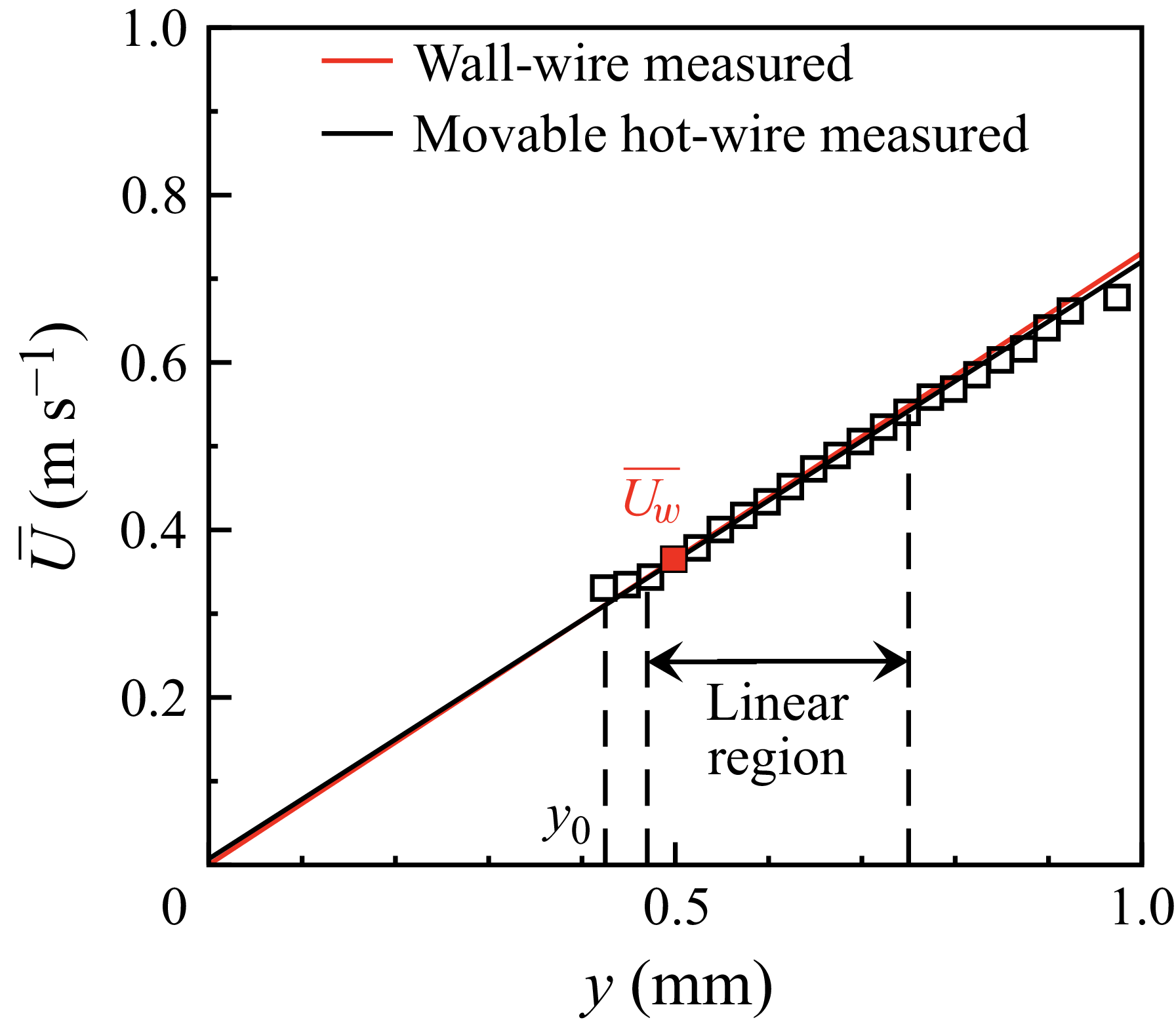
 ◼

 U+¯
 urms+


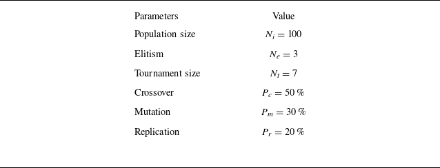
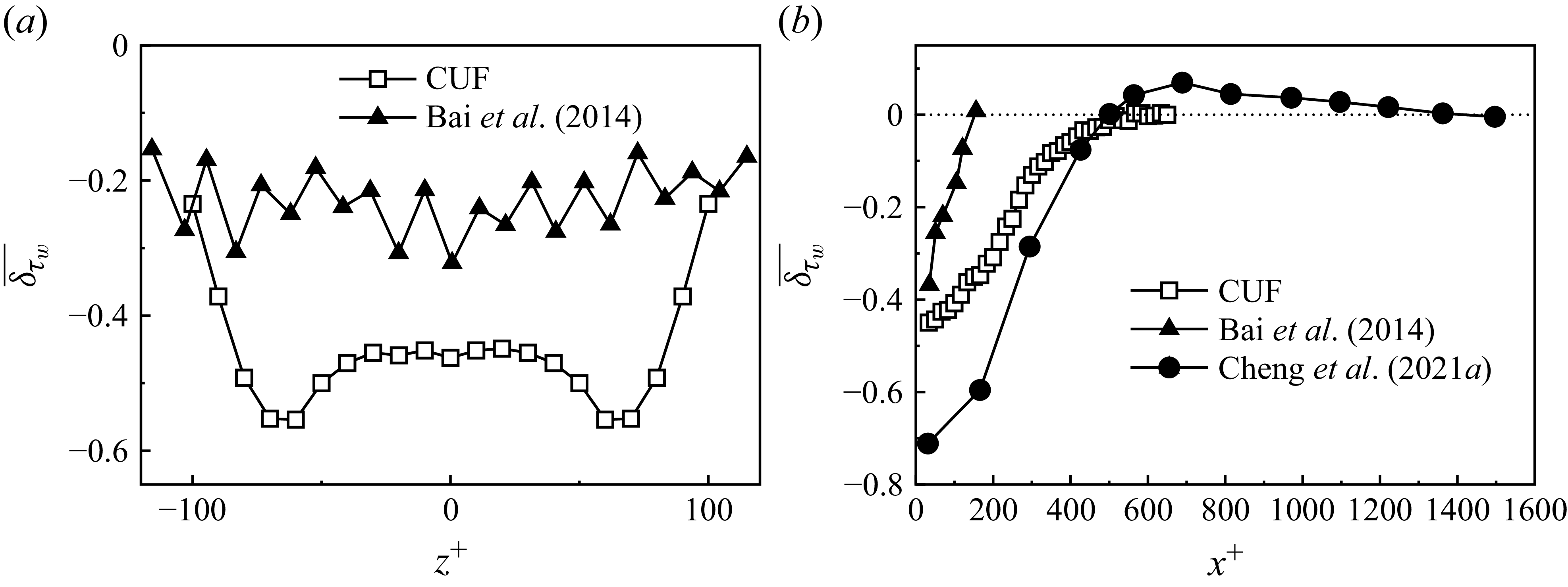
 δτw¯
 δτw¯
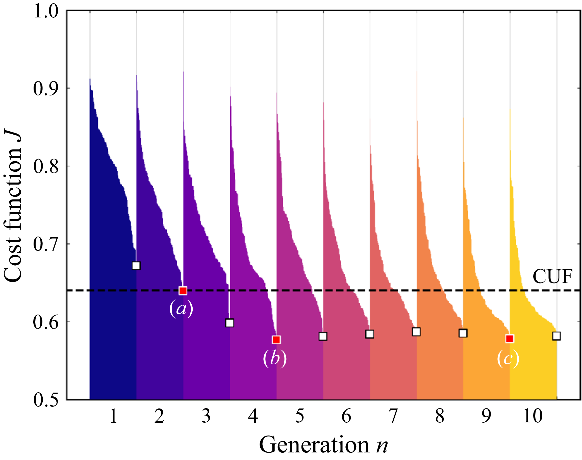
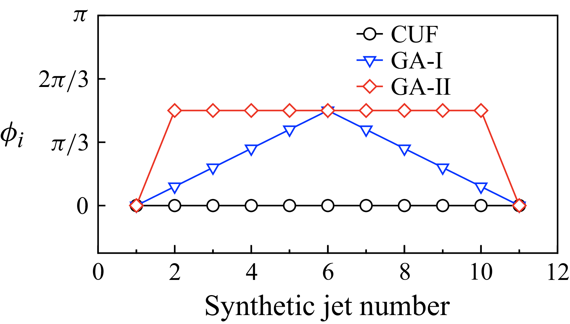
 ϕi

 δτw¯

 δτw¯


 ϕi


 W+¯
 V+¯
 W+¯
 W+¯
 ⟨W¯⟩z+


 U+¯
 U∗¯


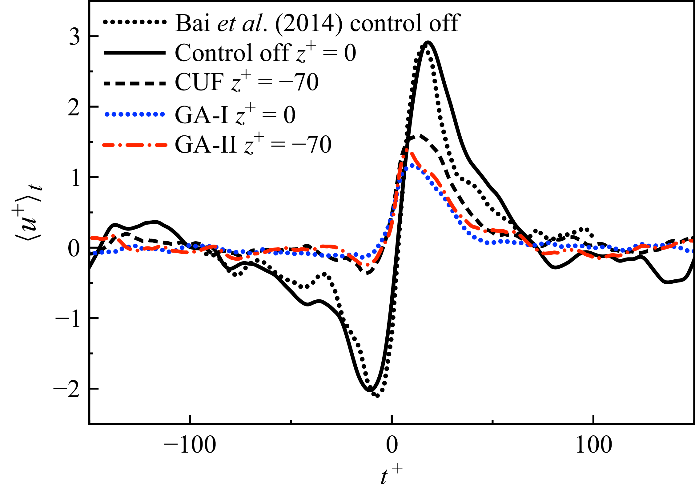

 (du/dy)2¯
 −uv¯(dU¯/dy)

 δτw
 δτw~


