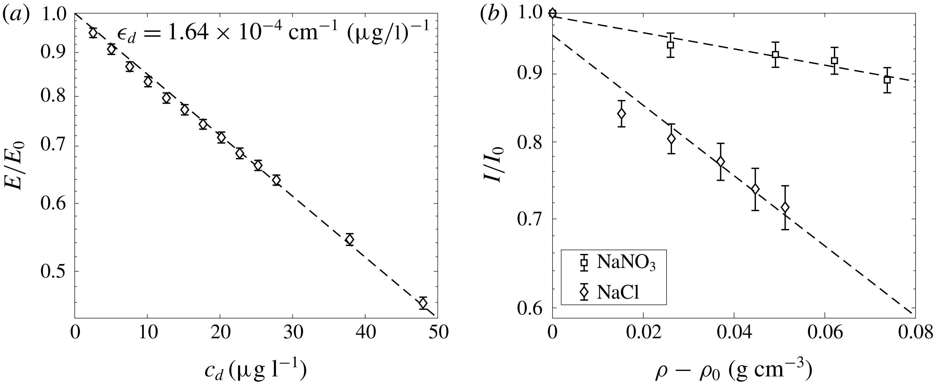
1 Introduction
Buoyancy-driven wall-bounded flows occur in both natural environments and industrial situations. The presence of a vertical wall in such flows is known to inhibit the process of turbulent entrainment (Lee & Emmons Reference Lee and Emmons1961) and thereby affect the mixing that arises. Here we investigate the effects of introducing a vertical wall to the flow generated by a line source of buoyancy. Applicable flows within effectively unbounded environments include the descending ‘free’ plume resulting from a chilled ceiling beam in the middle of a room, wherein the mixing of the plume affects the resulting thermal conditions within the room. In this paper we investigate the entrainment mechanisms and determine the extent to which the mixing of such plumes is altered if a chilled ceiling beam was placed adjacent to a wall, thereby producing a ‘wall plume’.
A broad finding among the early studies of wall plumes (Ellison & Turner Reference Ellison and Turner1959; Lee & Emmons Reference Lee and Emmons1961; Turner Reference Turner1973) is that the entrainment rates are significantly lower than those found in free plumes. Although velocity or buoyancy profile measurements were not presented in these studies, it was suggested that the wall suppresses the formation of large-scale structures and inhibits mixing, resulting in reduced entrainment into the plume. Velocity and buoyancy profiles are presented in later studies by Grella & Faeth (Reference Grella and Faeth1975) and Lai & Faeth (Reference Lai and Faeth1987), but in regions relatively close to the source where the flow was not self-similar. The only experimental velocity and buoyancy measurements of a wall plume in a self-similar region are those of Sangras, Dai & Faeth (Reference Sangras, Dai and Faeth1998) and Sangras, Dai & Faeth (Reference Sangras, Dai and Faeth2000), but they did not present simultaneous measurements. Nevertheless, the early findings of a reduced entrainment coefficient were confirmed, and entrainment approximately half that of a free plume was observed (Sangras et al. Reference Sangras, Dai and Faeth1998). This reduction in entrainment was largely attributed to the reduced meandering of the large-scale structures and suppression of cross-stream turbulent fluxes (Ellison & Turner Reference Ellison and Turner1959; Turner Reference Turner1973; Sangras et al. Reference Sangras, Dai and Faeth2000).
Despite these insights, to our knowledge, a study examining and comparing the large-scale structures and cross-stream turbulent fluxes of a wall plume to those of a free plume does not exist. However, much attention has recently been devoted to turbulent entrainment in other free-shear and wall-bounded flows, providing a framework which may be extended to wall plumes. Based on the formalism of Priestley & Ball (Reference Priestley and Ball1955), Paillat & Kaminski (Reference Paillat and Kaminski2014b
) suggested an entrainment model for turbulent plane jets, later extended to turbulent plane plumes by Paillat & Kaminski (Reference Paillat and Kaminski2014a
) where relative contributions of turbulent production,
 $\unicode[STIX]{x1D6FC}_{production}$
, and net buoyancy,
 $\unicode[STIX]{x1D6FC}_{buoyant}$
, to the entrainment coefficient could be distinguished and quantified. A similar decomposition was performed by van Reeuwijk & Craske (Reference van Reeuwijk and Craske2015) for a turbulent axisymmetric plume and by Holzner, van Reeuwijk & Jonker (Reference Holzner, van Reeuwijk and Jonker2016) on turbulent entrainment in an inclined gravity current, where the contribution from the viscous terms,
 $\unicode[STIX]{x1D6FC}_{viscous}$
, which are non-negligible due to the viscous boundary layer was also calculated but found to be relatively small compared to the combined contributions of turbulent production and net buoyancy.
Other studies have sought to understand turbulent flows by examining the small-scale processes ultimately responsible for turbulent entrainment (Philip et al. Reference Philip, Meneveau, de Silva and Marusic2014) by considering the entrainment across surfaces within the flow and relating this to the bulk entrainment. In doing so, some authors have attempted to disentangle dominant large-scale processes, whereby ambient fluid is ‘engulfed’ by the plume, with small-scale processes close to the turbulent/non-turbulent interface (TNTI) termed ‘nibbling’, whereby vorticity is imparted to the ambient fluid via viscous stresses across the TNTI at a length scale close to the Taylor microscale (Terashima et al. Reference Terashima, Sakai, Nagata, Ito, Onishi and Shouji2016). While Philip et al. (Reference Philip, Meneveau, de Silva and Marusic2014) suggest that large-scale eddies determine the overall rate of entrainment, Westerweel et al. (Reference Westerweel, Fukushima, Pedersen and Hunt2009) conclude that the entrainment process is dominated by ‘nibbling’. However, it is agreed that mixing is greatly enhanced due to stretching of surfaces by vorticity (Ottino Reference Ottino1989). By experimentally examining a turbulent jet Mistry et al. (Reference Mistry, Philip, Dawson and Marusic2016) show that turbulent entrainment in jets is a multi-scale process where at large-scale ambient fluid is transported across smooth surfaces, but ultimately transported across the TNTI, which exhibits fractal qualities, at smaller scales at relatively low velocities. This is consistent with Meneveau & Sreenivasan (Reference Meneveau and Sreenivasan1990) who suggested that the total flux across the TNTI should be independent of scale. Burridge et al. (Reference Burridge, Parker, Kruger, Partridge and Linden2017) examined an axisymmetric plume and suggested that engulfment of ambient fluid by the large-scale structures is the rate-limiting process for turbulent entrainment, consistent with Philip et al. (Reference Philip, Meneveau, de Silva and Marusic2014).
In this paper we use an energy decomposition to examine the reduced entrainment in a wall plume. We follow the free plume entrainment decomposition developed by Paillat & Kaminski (Reference Paillat and Kaminski2014a ) and extend the theory to a wall plume, which closely follows the entrainment decomposition of Holzner et al. (Reference Holzner, van Reeuwijk and Jonker2016) in an inclined turbulent gravity current, where relative contributions of turbulent production, buoyancy and viscous terms may be calculated directly. In doing so relative contributions to the entrainment coefficient may be compared between the free and wall plume. We also use methods developed by Mistry et al. (Reference Mistry, Philip, Dawson and Marusic2016) and Burridge et al. (Reference Burridge, Parker, Kruger, Partridge and Linden2017) to examine the statistics of the TNTI by both quantifying the increased meandering in a free plume and relating this to the increased length of the TNTI in the free plume. This is achieved by making simultaneous measurements of velocity and buoyancy in self-similar line plumes adjacent to and far from a vertical wall.
The paper is organised as follows. We review plume theory for two-dimensional free and wall plumes and the results of previous studies and extend the entrainment decomposition of Paillat & Kaminski (Reference Paillat and Kaminski2014a ) to wall plumes in § 2. The experimental methods and data analysis are presented in § 3, and the validation of the data is described in § 4. The experimental results are presented and discussed in an Eulerian coordinate system in § 5 and in a plume coordinate system in § 6. Finally, the conclusions are presented in § 7.
2 Theory and previous work on entrainment in free and wall plumes
A turbulent line plume is the flow driven by an infinitely long horizontal line source of buoyancy. The wall plume differs from the free plume by the presence of a vertical wall that is placed immediately adjacent to, and spans the entire length of, the line source. We consider a uniform ambient fluid and restrict attention to the case where the wall is adiabatic so that there is no loss nor addition of buoyancy into the plume. Consequently, the buoyancy flux is constant with height in both the free plume and the wall plume. Here we outline the theory of entrainment in free and wall plumes in a quiescent environment and adapt the entrainment coefficient decomposition of free plumes developed by Paillat & Kaminski (Reference Paillat and Kaminski2014a ) to wall plumes.
In both flows we define the velocity
 $w(x,z,t)$
in the vertical
 $z$
-direction, horizontal velocity
 $u(x,z,t)$
in the across-plume
 $x$
-direction and the buoyancy
 $b(x,z,t)=g(\unicode[STIX]{x1D70C}_{a}-\unicode[STIX]{x1D70C}(x,z,t))/\unicode[STIX]{x1D70C}_{a}$
, where
 $\unicode[STIX]{x1D70C}$
and
 $\unicode[STIX]{x1D70C}_{a}$
are the density of the plume and ambient, respectively. Since the flows are statistically steady, these quantities may be decomposed into time-averaged and fluctuating components
 $w(x,z,t)=\overline{w}(x,z)+w^{\prime }(x,z,t)$
,
 $u(x,z,t)=\overline{u}(x,z)+u^{\prime }(x,z,t)$
and
 $b(x,z,t)=\overline{b}(x,z)+b^{\prime }(x,z,t)$
, and we denote the time-averaged maximum vertical velocity and buoyancy as
 $\overline{w}_{m}(z)$
and
 $\overline{b}_{m}(z)$
. We assume all quantities are independent of the
 $y$
-direction aligned along the plume source. Under the Boussinesq approximation, the simplified Reynolds time-averaged mass, momentum and buoyancy conservation equations may be written as
 $$\begin{eqnarray}\displaystyle & \displaystyle \frac{\unicode[STIX]{x2202}\overline{u}}{\unicode[STIX]{x2202}x}+\frac{\unicode[STIX]{x2202}\overline{w}}{\unicode[STIX]{x2202}z}=0, & \displaystyle\end{eqnarray}$$
 $$\begin{eqnarray}\displaystyle & \displaystyle \overline{u}\frac{\unicode[STIX]{x2202}\overline{w}}{\unicode[STIX]{x2202}x}+\overline{w}\frac{\unicode[STIX]{x2202}\overline{w}}{\unicode[STIX]{x2202}z}=\overline{b}-\frac{\unicode[STIX]{x2202}\overline{u^{\prime }w^{\prime }}}{\unicode[STIX]{x2202}x}+\unicode[STIX]{x1D708}\frac{\unicode[STIX]{x2202}^{2}\overline{w}}{\unicode[STIX]{x2202}x^{2}}, & \displaystyle\end{eqnarray}$$
 $$\begin{eqnarray}\displaystyle & \displaystyle \overline{u}\frac{\unicode[STIX]{x2202}\overline{b}}{\unicode[STIX]{x2202}x}+\overline{w}\frac{\unicode[STIX]{x2202}\overline{b}}{\unicode[STIX]{x2202}z}=0, & \displaystyle\end{eqnarray}$$
where
 $\unicode[STIX]{x1D708}$
is the kinematic viscosity of the fluid. We define, respectively, the time-averaged volume flux, specific momentum flux, specific energy flux, integral buoyancy and buoyancy flux per unit length by
 $$\begin{eqnarray}Q_{f}(z)=\int _{-\infty }^{\infty }\overline{w}(x,z)\,\text{d}x,\quad Q_{w}(z)=\int _{0}^{\infty }\overline{w}(x,z)\,\text{d}x,\end{eqnarray}$$
 $$\begin{eqnarray}M_{f}(z)=\int _{-\infty }^{\infty }\overline{w}^{2}(x,z)\,\text{d}x,\quad M_{w}(z)=\int _{0}^{\infty }\overline{w}^{2}(x,z)\,\text{d}x,\end{eqnarray}$$
 $$\begin{eqnarray}E_{f}(z)=\int _{-\infty }^{\infty }\overline{w}^{3}(x,z)\,\text{d}x,\quad E_{w}(z)=\int _{0}^{\infty }\overline{w}^{3}(x,z)\,\text{d}x,\end{eqnarray}$$
 $$\begin{eqnarray}B_{f}(z)=\int _{-\infty }^{\infty }\overline{b}(x,z)\,\text{d}x,\quad B_{w}(z)=\int _{0}^{\infty }\overline{b}(x,z)\,\text{d}x,\end{eqnarray}$$
 $$\begin{eqnarray}F_{f}(z)=\int _{-\infty }^{\infty }\overline{w}(x,z)\overline{b}(x,z)\,\text{d}x,\quad F_{w}(z)=\int _{0}^{\infty }\overline{w}(x,z)\overline{b}(x,z)\,\text{d}x,\end{eqnarray}$$
where the suffices
 $f$
and
 $w$
denote the free and wall plumes, respectively. In addition, we define the source buoyancy flux per unit length as
 $F_{0}$
. From these relations we define the characteristic scales for plume width
 $R$
and velocity
 $W$
by
 $$\begin{eqnarray}R_{f}=\frac{Q_{f}^{2}}{2M_{f}},\quad R_{w}=\frac{Q_{w}^{2}}{M_{w}},\end{eqnarray}$$
 $$\begin{eqnarray}W_{f}=\frac{M_{f}}{Q_{f}},\quad W_{w}=\frac{M_{w}}{Q_{w}}.\end{eqnarray}$$
Note that in the case of the free plume,
 $R_{f}$
is equivalent to a ‘top-hat’ half-width, whereas for the wall plume,
 $R_{w}$
is equivalent to a ‘top-hat’ full-width, which is used since it is analogous to the half-width of the free plume.
For the free plume, by assuming high Reynolds number, the last term in (2.2) may be ignored. Using the entrainment assumption, that the inflow velocity at any height is proportional to the local vertical plume velocity i.e.
 $u(-\infty ,z)=-u(\infty ,z)=\unicode[STIX]{x1D6FC}_{f}W_{f}$
, where
 $\unicode[STIX]{x1D6FC}_{f}$
is the ‘top-hat’ entrainment coefficient (Morton, Taylor & Turner Reference Morton, Taylor and Turner1956), the integration of equations (2.1)–(2.3), with the boundary conditions
 $\overline{w}(-\infty ,z)=\overline{u^{\prime }w^{\prime }}(-\infty ,z)=\overline{w}(\infty ,z)=\overline{u^{\prime }w^{\prime }}(\infty ,z)=0$
, gives the free plume conservation equations for the time-averaged volume, momentum and buoyancy flux
 $$\begin{eqnarray}\displaystyle & \displaystyle \frac{\text{d}Q_{f}}{\text{d}z}=2\unicode[STIX]{x1D6FC}_{f}\frac{M_{f}}{Q_{f}}, & \displaystyle\end{eqnarray}$$
 $$\begin{eqnarray}\displaystyle & \displaystyle \frac{\text{d}M_{f}}{\text{d}z}=B_{f}=\frac{\unicode[STIX]{x1D703}_{f}F_{f}Q_{f}}{M_{f}}, & \displaystyle\end{eqnarray}$$
 $$\begin{eqnarray}\displaystyle & \displaystyle \frac{\text{d}F_{f}}{\text{d}z}=0, & \displaystyle\end{eqnarray}$$
where
 $\unicode[STIX]{x1D703}_{f}$
encapsulates the relation between the integral buoyancy
 $B_{f}$
and the buoyancy flux
 $F_{f}$
, which by assuming self-similarity we may take as constant. Note that in (2.11) the factor of two occurs as
 $\unicode[STIX]{x1D6FC}_{f}$
is the entrainment into one side of the plume only. The solutions to the free plume equations (2.11)–(2.13) are
 $$\begin{eqnarray}\displaystyle & \displaystyle Q_{f}(z)=\left(2\unicode[STIX]{x1D6FC}_{f}\right)^{2/3}\left(\unicode[STIX]{x1D703}_{f}F_{f}\right)^{1/3}z, & \displaystyle\end{eqnarray}$$
 $$\begin{eqnarray}\displaystyle & \displaystyle M_{f}(z)=\left(2\unicode[STIX]{x1D6FC}_{f}\right)^{1/3}\left(\unicode[STIX]{x1D703}_{f}F_{f}\right)^{2/3}z, & \displaystyle\end{eqnarray}$$
 $$\begin{eqnarray}\displaystyle & \displaystyle F_{f}(z)=F_{f}. & \displaystyle\end{eqnarray}$$
For the wall plume the viscous term in (2.2) is assumed to be non-negligible as it characterises the effect of the no-slip boundary condition on the wall. Using the same entrainment assumption that
 $u(\infty ,z)=-\unicode[STIX]{x1D6FC}_{w}W_{w}$
, the integration of equations (2.1)–(2.3) with the boundary conditions
 $\overline{w}(0,z)=\overline{u}(0,z)=\overline{u^{\prime }w^{\prime }}(0,z)=\overline{w}(\infty ,z)=\overline{u^{\prime }w^{\prime }}(\infty ,z)=0$
gives the wall plume conservation equations for the time-averaged volume, momentum and buoyancy flux
 $$\begin{eqnarray}\displaystyle & \displaystyle \frac{\text{d}Q_{w}}{\text{d}z}=\unicode[STIX]{x1D6FC}_{w}\frac{M_{w}}{Q_{w}}, & \displaystyle\end{eqnarray}$$
 $$\begin{eqnarray}\displaystyle & \displaystyle \frac{\text{d}M_{w}}{\text{d}z}=B_{w}-\left.\unicode[STIX]{x1D708}\frac{\unicode[STIX]{x2202}w}{\unicode[STIX]{x2202}x}\right|_{0}=\frac{\unicode[STIX]{x1D703}_{w}F_{w}Q_{w}}{M_{w}}-C\left(\frac{M_{w}}{Q_{w}}\right)^{2}, & \displaystyle\end{eqnarray}$$
 $$\begin{eqnarray}\displaystyle & \displaystyle \frac{\text{d}F_{w}}{\text{d}z}=0, & \displaystyle\end{eqnarray}$$
where
 $\unicode[STIX]{x1D703}_{w}$
encapsulates the relation between the integral buoyancy
 $B_{w}$
and the buoyancy flux
 $F_{w}$
, and we express the wall shear stress in terms of the characteristic velocity
 $W_{w}$
and a (constant) skin friction coefficient
 $C$
. The assumption of self-similarity in the wall plume is more problematic because of the existence of a viscous boundary layer in order to satisfy the no-slip condition on the vertical wall. However, throughout this paper we assume that the wall plume is self-similar, an assumption which we show to be valid in § 4. Therefore, we take
 $\unicode[STIX]{x1D703}_{w}$
and
 $C$
to be constants. The solutions to the wall plume equations (2.17)–(2.19) are
 $$\begin{eqnarray}\displaystyle & \displaystyle Q_{w}(z)=\left(\frac{\unicode[STIX]{x1D703}_{w}F_{w}}{1+{\displaystyle \frac{C}{\unicode[STIX]{x1D6FC}_{w}}}}\right)^{1/3}\unicode[STIX]{x1D6FC}_{w}^{2/3}z, & \displaystyle\end{eqnarray}$$
 $$\begin{eqnarray}\displaystyle & \displaystyle M_{w}(z)=\left(\frac{\unicode[STIX]{x1D703}_{w}F_{w}}{1+{\displaystyle \frac{C}{\unicode[STIX]{x1D6FC}_{w}}}}\right)^{2/3}\unicode[STIX]{x1D6FC}_{w}^{1/3}z, & \displaystyle\end{eqnarray}$$
 $$\begin{eqnarray}\displaystyle & \displaystyle F_{w}(z)=F_{w}. & \displaystyle\end{eqnarray}$$
The constants
 $\unicode[STIX]{x1D6FC}_{w}$
and
 $\unicode[STIX]{x1D6FC}_{f}$
are the standard top-hat entrainment coefficients. However, it has been widely observed in previous studies that the vertical velocity and buoyancy profiles of a free plume are well fitted by a Gaussian curve, (e.g. Ramaprian & Chandrasekhara Reference Ramaprian and Chandrasekhara1989; Paillat & Kaminski Reference Paillat and Kaminski2014a
) and conservation of volume flux in the free and wall plume may also be expressed in terms of the maximum vertical velocity and a Gaussian entrainment coefficient
 $\unicode[STIX]{x1D6FC}_{G}$
, in the form
 $$\begin{eqnarray}\frac{\text{d}Q_{f}}{\text{d}z}=2\unicode[STIX]{x1D6FC}_{f,G}\overline{w}_{m},\quad \frac{\text{d}Q_{w}}{\text{d}z}=\unicode[STIX]{x1D6FC}_{w,G}\overline{w}_{m}.\end{eqnarray}$$
The top-hat entrainment coefficient in the free plume is related to the Gaussian coefficient by
 $\unicode[STIX]{x1D6FC}_{f}=\sqrt{2}\,\unicode[STIX]{x1D6FC}_{f,G}$
and most studies choose to calculate
 $\unicode[STIX]{x1D6FC}_{f,G}$
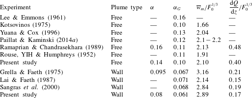
. At present there is significant disagreement about the value of the entrainment coefficient, with previously reported Gaussian entrainment values in the range
 $\unicode[STIX]{x1D6FC}_{f,G}=\{0.10,0.16\}$
(table 1).
Entrainment values, scaled vertical velocities and scaled rate of change of mean volume flux of previous work, where
 $F_{0}$
is the source buoyancy flux.
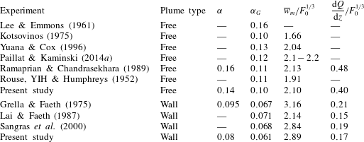
Most studies on wall plumes also focus on the Gaussian entrainment coefficient
 $\unicode[STIX]{x1D6FC}_{w,G}$
, although in some cases, notably Grella & Faeth (Reference Grella and Faeth1975), the top-hat value
 $\unicode[STIX]{x1D6FC}_{w}$
was also calculated. Since the velocity profile of the wall plume is not a known analytic function a theoretical relation between
 $\unicode[STIX]{x1D6FC}_{w}$
and
 $\unicode[STIX]{x1D6FC}_{w,G}$
cannot be derived, although Grella & Faeth (Reference Grella and Faeth1975) find that
 $\unicode[STIX]{x1D6FC}_{w}/\unicode[STIX]{x1D6FC}_{w,G}\approx 1.4$
. There is broad agreement with previously measured Gaussian entrainment values of the wall plume (table 1). This is somewhat surprising given the additional difficulties associated with measuring the velocity of the wall plume, which is perhaps reflected in the variation in other parameters between these experiments, especially the maximum mean velocity used in the calculation of
 $\unicode[STIX]{x1D6FC}_{w,G}$
. Further, Grella & Faeth (Reference Grella and Faeth1975) and Lai & Faeth (Reference Lai and Faeth1987) emphasise that their data were not in a self-similar region as the flow appeared to be evolving over the whole range of heights where the measurements were taken. For these reasons it appears that, to our knowledge, an experimentally determined top-hat entrainment value for a wall plume within a self-similar region does not exist in the literature. This is problematic given the unknown relationship between
 $\unicode[STIX]{x1D6FC}_{w,G}$
and
 $\unicode[STIX]{x1D6FC}_{w}$
in a self-similar region and that, despite the consistency between the previously determined
 $\unicode[STIX]{x1D6FC}_{w,G}$
, the closure model of (2.23) relies on an established maximum velocity for which there is significant disagreement.
Our study is focused on the comparison of the top-hat entrainment values for a free and a wall plume. Since these two flows have different velocity profiles it is natural to compare the entrainment rates without any assumption on profile shapes. It is, therefore, unfortunate that for the wall plume case previous work has paid less attention to the top-hat value.
2.1 Energy decomposition of entrainment in turbulent wall plumes
Paillat & Kaminski (Reference Paillat and Kaminski2014a ) used the formalism of Priestley & Ball (Reference Priestley and Ball1955) and Kaminski, Tait & Carazzo (Reference Kaminski, Tait and Carazzo2005) to develop a theoretical model of entrainment in free turbulent plumes, which had previously been adapted to free turbulent planar jets by Paillat & Kaminski (Reference Paillat and Kaminski2014b ). This involved decomposing the entrainment coefficient into relative contributions from buoyancy and turbulent production. A similar analysis has also been performed on turbulent inclined gravity currents by Holzner et al. (Reference Holzner, van Reeuwijk and Jonker2016), where the contributions from the viscous terms due to the wall were also included and found to be small compared to the buoyant and turbulent production terms. Here we outline a similar decomposition of the entrainment coefficient of the wall plume into separate turbulent production, buoyant and viscous terms.
An expression for the conservation of vertical kinetic energy may be obtained by multiplying (2.2) by
 $\overline{w}$
and using the continuity equation to obtain (Priestley & Ball Reference Priestley and Ball1955),
 $$\begin{eqnarray}\frac{\unicode[STIX]{x2202}}{\unicode[STIX]{x2202}z}\left(\frac{1}{2}\overline{w}^{3}\right)+\frac{\unicode[STIX]{x2202}}{\unicode[STIX]{x2202}x}\left(\frac{1}{2}\overline{u}~\overline{w}^{2}\right)=\overline{w}\overline{b}-\overline{w}\frac{\unicode[STIX]{x2202}}{\unicode[STIX]{x2202}x}\left(\overline{u^{\prime }w^{\prime }}\right)+\unicode[STIX]{x1D708}\overline{w}\frac{\unicode[STIX]{x2202}^{2}\overline{w}}{\unicode[STIX]{x2202}x^{2}},\end{eqnarray}$$
where integrating with the wall plume boundary conditions gives
 $$\begin{eqnarray}\frac{\text{d}E_{w}}{\text{d}z}=2F_{w}+2\int _{0}^{\infty }\frac{\unicode[STIX]{x2202}\overline{w}}{\unicode[STIX]{x2202}x}\overline{u^{\prime }w^{\prime }}\,\text{d}x-2\unicode[STIX]{x1D708}\int _{0}^{\infty }\left(\frac{\unicode[STIX]{x2202}\overline{w}}{\unicode[STIX]{x2202}x}\right)^{2}\,\text{d}x.\end{eqnarray}$$
The conservation of volume flux may be expressed as follows (Paillat & Kaminski Reference Paillat and Kaminski2014a )
 $$\begin{eqnarray}\frac{\text{d}Q_{w}}{\text{d}z}=2\frac{Q_{w}}{M_{w}}\frac{\text{d}M_{w}}{\text{d}z}-\frac{Q_{w}}{E_{w}}\frac{\text{d}E_{w}}{\text{d}z}+\frac{M_{w}^{2}}{E_{w}}\frac{\text{d}}{\text{d}z}\left(\frac{Q_{w}E_{w}}{M_{w}^{2}}\right),\end{eqnarray}$$
where, assuming self-similarity, the last term is zero. By equating (2.17) and (2.26) the entrainment coefficient may be expressed as
 $$\begin{eqnarray}\unicode[STIX]{x1D6FC}_{w}=2\frac{Q_{w}^{2}}{M_{w}^{2}}\frac{\text{d}M_{w}}{\text{d}z}-\frac{Q_{w}^{2}}{E_{w}M_{w}}\frac{\text{d}E_{w}}{\text{d}z},\end{eqnarray}$$
and substituting equation (2.18) and (2.25) into (2.27) gives
 $$\begin{eqnarray}\unicode[STIX]{x1D6FC}_{w}=\unicode[STIX]{x1D6FC}_{buoyant}+\unicode[STIX]{x1D6FC}_{production}+\unicode[STIX]{x1D6FC}_{viscous},\end{eqnarray}$$
where
 $$\begin{eqnarray}\displaystyle & \displaystyle \unicode[STIX]{x1D6FC}_{buoyant}=2Ri\left(\unicode[STIX]{x1D703}_{w}-\frac{M_{w}^{2}}{Q_{w}E_{w}}\right), & \displaystyle\end{eqnarray}$$
 $$\begin{eqnarray}\displaystyle & \displaystyle \unicode[STIX]{x1D6FC}_{production}=-2\frac{Q_{w}^{2}}{E_{w}M_{w}}\int _{0}^{\infty }\frac{\unicode[STIX]{x2202}\overline{w}}{\unicode[STIX]{x2202}x}\overline{u^{\prime }w^{\prime }}\,\text{d}x, & \displaystyle\end{eqnarray}$$
 $$\begin{eqnarray}\displaystyle & \displaystyle \unicode[STIX]{x1D6FC}_{viscous}=\frac{2Q^{2}\unicode[STIX]{x1D708}}{E_{w}M_{w}}\int _{0}^{\infty }\left(\frac{\unicode[STIX]{x2202}\overline{w}}{\unicode[STIX]{x2202}x}\right)^{2}\,\text{d}x-2C, & \displaystyle\end{eqnarray}$$
and
 $Ri$
is the Richardson number defined by
 $Ri=F_{w}Q_{w}^{3}/M_{w}^{3}$
. The first term,
 $\unicode[STIX]{x1D6FC}_{buoyant}$
, may be interpreted as the net effect of buoyancy contributing to entrainment which, as noted by van Reeuwijk & Craske (Reference van Reeuwijk and Craske2015), provides plumes with a mechanism for entrainment not directly associated with turbulence. The second term,
 $\unicode[STIX]{x1D6FC}_{production}$
, corresponds to the efficiency of turbulent entrainment driven by the turbulent production (Paillat & Kaminski Reference Paillat and Kaminski2014a
) and
 $\unicode[STIX]{x1D6FC}_{viscous}$
corresponds to the inner boundary layer processes that require energy but are not directly related to entrainment (Holzner et al.
Reference Holzner, van Reeuwijk and Jonker2016).
A similar decomposition of the free plume entrainment coefficient gives (Paillat & Kaminski Reference Paillat and Kaminski2014a )
 $$\begin{eqnarray}\unicode[STIX]{x1D6FC}_{f}=\unicode[STIX]{x1D6FC}_{buoyant}+\unicode[STIX]{x1D6FC}_{production},\end{eqnarray}$$
where
 $$\begin{eqnarray}\displaystyle & \displaystyle \unicode[STIX]{x1D6FC}_{buoyant}=Ri\left(\unicode[STIX]{x1D703}_{f}-\frac{M_{f}^{2}}{Q_{f}E_{f}}\right), & \displaystyle\end{eqnarray}$$
 $$\begin{eqnarray}\displaystyle & \displaystyle \unicode[STIX]{x1D6FC}_{production}=-\frac{Q_{f}^{2}}{E_{f}M_{f}}\int _{0}^{\infty }\frac{\unicode[STIX]{x2202}\overline{w}}{\unicode[STIX]{x2202}x}\overline{u^{\prime }w^{\prime }}\,\text{d}x, & \displaystyle\end{eqnarray}$$
and
 $Ri$
is the Richardson number, similarly defined by
 $Ri=F_{f}Q_{f}^{3}/M_{f}^{3}$
and the decomposed terms may be interpreted as above for the wall plume. Using experimental data we show the validity of the decomposition of the free plume, also shown by Paillat & Kaminski (Reference Paillat and Kaminski2014a
), and we calculate the relative contributions to the entrainment coefficient for the wall plume.
3 Experiments and analysis
3.1 Experimental details
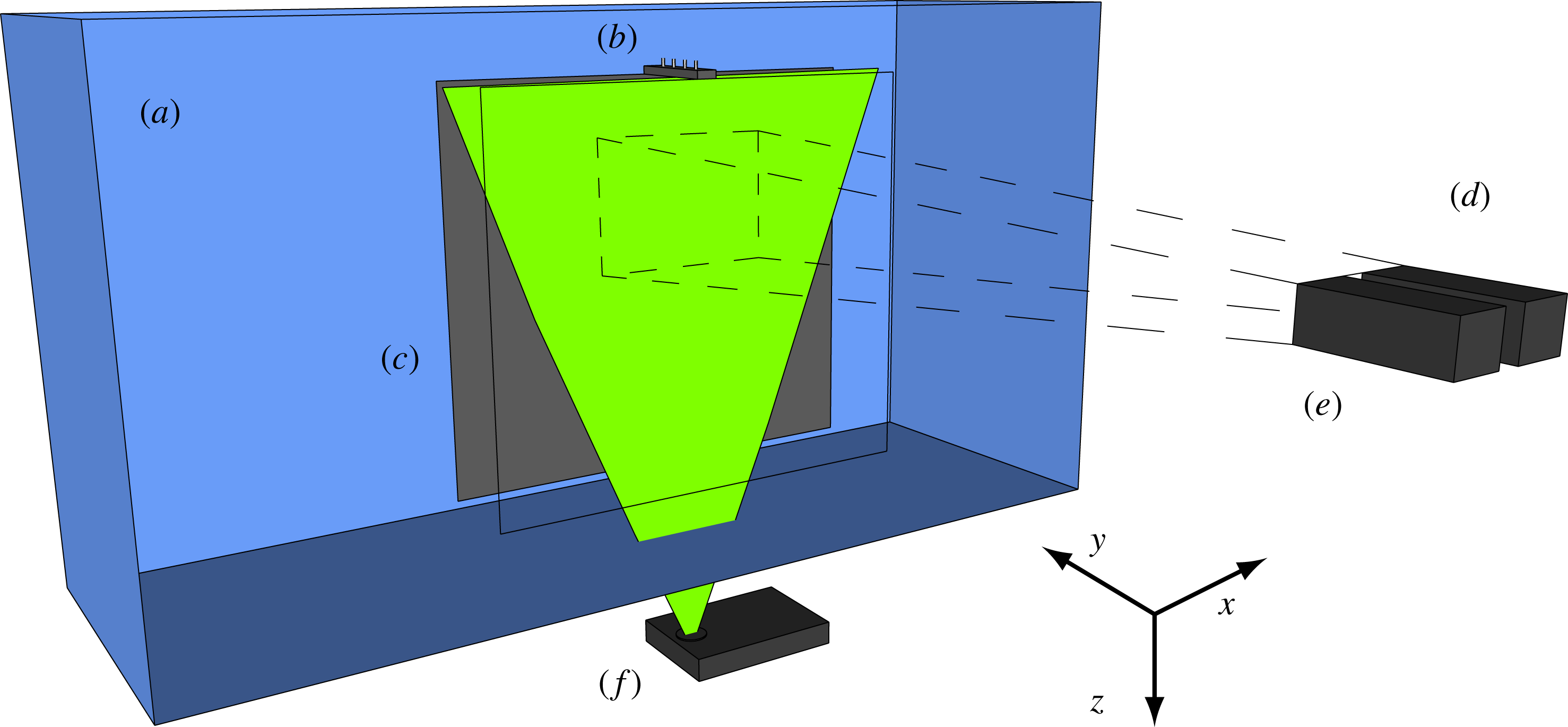
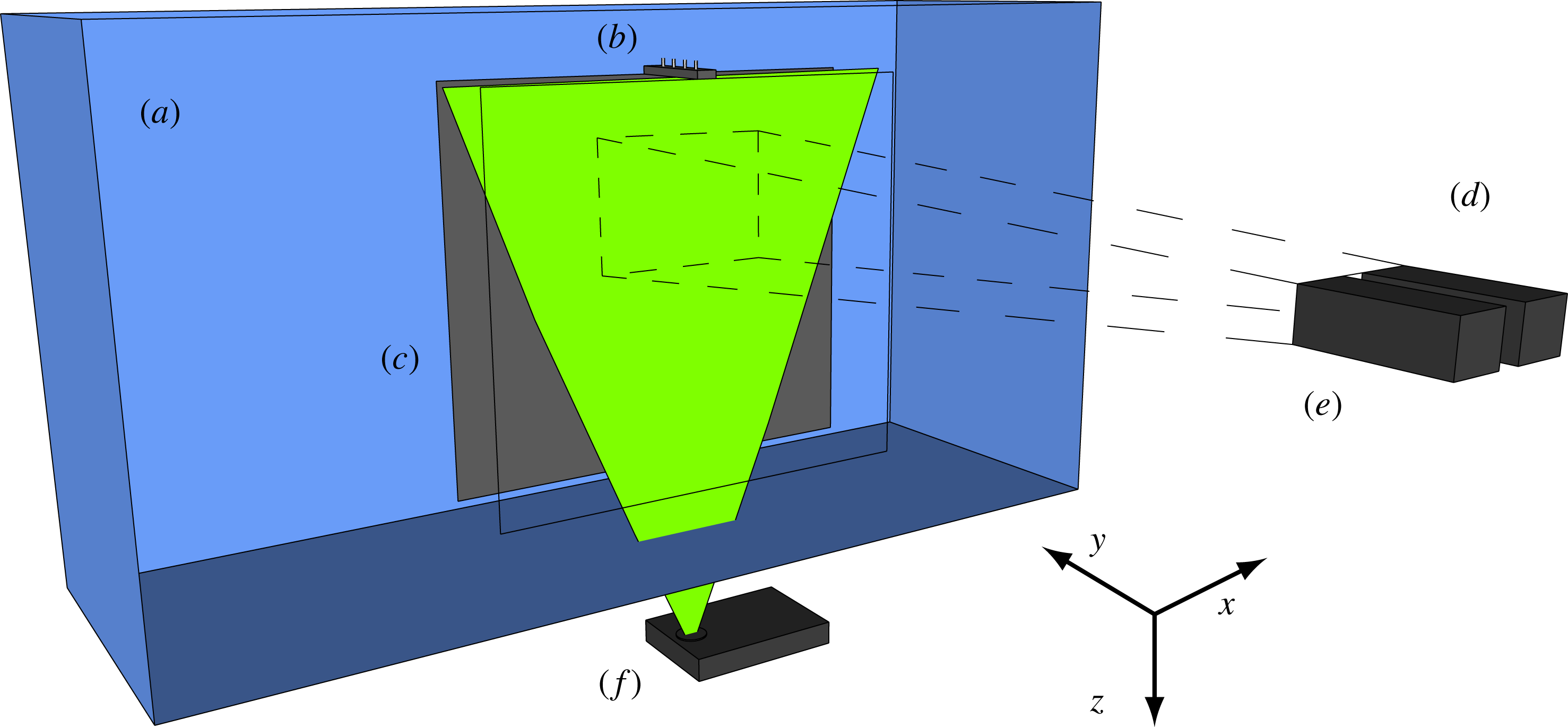
Diagram of the experimental set-up for the free plume showing the (a) water tank, (b) line source, (c) bounding walls perpendicular to the line source (see text), (d) PIV camera, (e) LIF camera and (f) laser. The illuminated plane (green) created by the laser shows the plane that the measurements were taken, perpendicular to the line source. The experimental set-up for the wall plume experiments differ only by the presence of a wall immediately adjacent to the line source (figure 2).
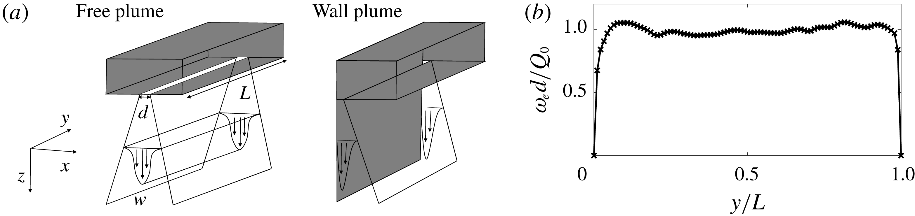
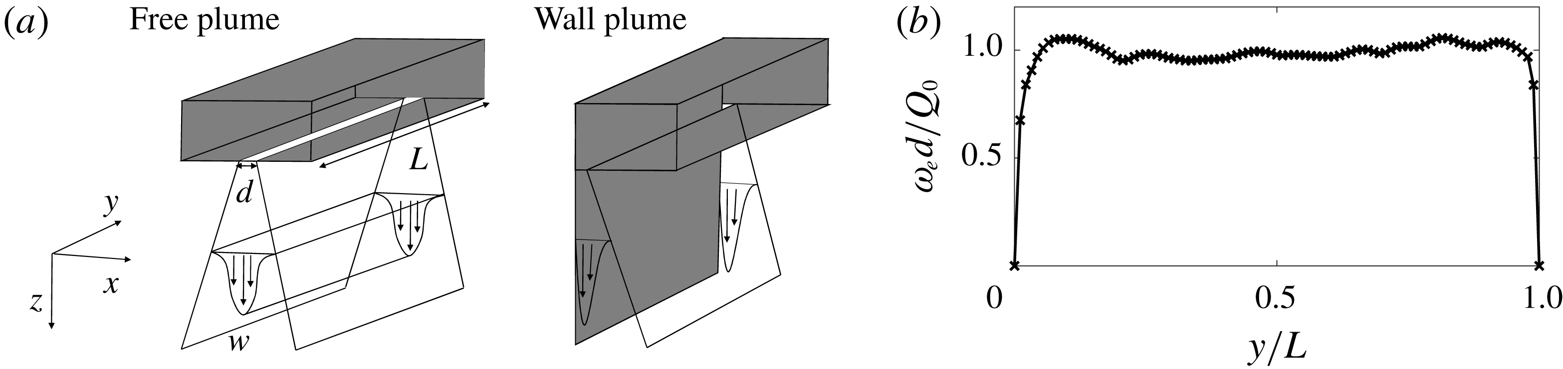
(a) The coordinate system of the free and wall plume and (b) the exit velocity, measured at 4 mm from the source exit, of the line source along the length of the source with a flow rate per unit length of
 $Q_{0}=1.00\times 10^{-4}~\text{m}^{2}~\text{s}^{-1}$
. The structures of the line source nozzle of the free and wall plumes were identical.
The experiments were designed to create turbulent free and wall plumes that would enable us to make simultaneous measurements of the buoyancy and velocity fields of the flow. The experiments were performed in a Perspex (acrylic) tank (figure 1) of horizontal cross-section
 $1.2~\text{m}\times 0.4~\text{m}$
filled with dilute saline solution of uniform density
 $\unicode[STIX]{x1D70C}_{a}$
to a depth of 0.75 m. Relatively dense sodium nitrate solution was used as source fluid which enabled refractive indices of the plume and ambient fluids to be matched as is needed for accurate measurements of the velocity and buoyancy field as described below. The source fluid, at a reduced gravity of
 $b_{0}$
, was supplied using a Cole-Parmer Digital Gear Pump System, 0.91 mL/rev, which was calibrated for each experiment with a separate flow rate. The gear pump provided uniform volume,
 $Q_{0}$
, and buoyancy,
 $F_{0}=Q_{0}b_{0}$
, fluxes per unit length, via a line source of dimension
 $L=0.15~\text{m}$
and width
 $d=1~\text{mm}$
. Figure 2(b) shows the line source exit velocity profile along the length of the source. The non-uniformity of the velocity profile is most prominent close to the walls, however, as highlighted by Krug et al. (Reference Krug, Holzner, Lüthi, Wolf, Kinzelbach and Tsinober2013) in their experimental investigation of a gravity current, the region close to the walls at
 $y/L=0$
and
 $y/L=1$
are subjected to boundary effects anyway so should not be of any additional concern with respect to the two-dimensional nature of the flow within the central region,
 $0.15<y/L<0.85$
, where the exit velocity varies by at most
 $6\,\%$
of the mean velocity. The initial density of the ambient and source fluid was measured using an Anton Paar DMA 5000 density meter to an accuracy of
 $1\times 10^{-3}~\text{kg}~\text{m}^{-3}$
, at
 $20\,^{\circ }\text{C}$
. The ambient and source solution were both left overnight to reach a uniform, and equal, temperature of
 $20\,^{\circ }\text{C}$
and were measured to be within
 $0.1\,^{\circ }\text{C}$
of this temperature. This corresponds to a maximum error of
 $0.15\,\%$
of the initial density differences used in our experiments. To promote the two-dimensionality of the flow by eliminating any entrainment from beyond the length of the source, the flow was enclosed by two
 $0.6~\text{m}\times 0.6~\text{m}$
transparent walls (
 $x$
–
 $z$
planes) perpendicular to the line source, separated by the length of the source, see figure 1. To create the wall plume a further vertical wall in the
 $y$
–
 $z$
plane was mounted immediately adjacent to one edge of the line source.
Simultaneous measurements of the velocity and density fields on a
 $x$
–
 $z$
plane were taken using particle image velocimetry (PIV) and laser induced fluorescence (LIF). A frequency-doubled dual-cavity Litron Nano L100 Nd:YAG pulsed laser with wavelength 532 nm was used to create a light sheet with a thickness of 1–2 mm in the measurement section. The illuminated sheet was then imaged using two AVT Bonito CMC-4000 4 megapixel CMOS cameras, as shown in figure 1. For the PIV measurements, polyamide particles with a mean diameter
 $2\times 10^{-2}~\text{mm}$
and density
 $1.02\times 10^{-3}~\text{kg}~\text{m}^{-3}$
were added to both the ambient and source fluid. To allow LIF measurements, a low concentration of the fluorescent dye Rhodamine 6G (
 $2\times 10^{-4}~\text{kg}~\text{m}^{-3}$
for all the experiments) was added to the source fluid. To separate the two signals, i.e. separate light scattered from the particles and that fluoresced by the dye, a narrow bandpass filter (centred at the wavelength of the laser) was placed in front of the PIV camera and a longpass filter was placed in front of the LIF camera. Images for both PIV and LIF were simultaneously captured at 100 Hz before being processed.
To determine the velocity fields, the raw particle images were processed using the 2017a PIV algorithm of Digiflow (Olsthoorn & Dalziel Reference Olsthoorn and Dalziel2017). Interrogation windows were chosen to be
 $24\times 24~\text{pixels}^{2}$
with an overlap of
 $50\,\%$
. Given the field of view of the camera, we were able to obtain one velocity vector every 1.12 mm and 1.09 mm for the free and wall plume, respectively. For the density field, given the low concentrations of Rhodamine 6G in the measurement section used (
 ${\sim}1\times 10^{-5}~\text{kg}~\text{m}^{-3}$
due to dilution through entrainment) a linear relationship between the light intensity perceived by the camera and the dye concentration was used to determine the density field as in Ferrier, Funk & Roberts (Reference Ferrier, Funk and Roberts1993). For the experiments described in this paper, a two-point calibration was performed for each experiment by capturing an image of the background light intensity and an image at a known dye concentration. Both calibration images were captured with the polyamide particles within the tank, at the seeding density used for the experiment, to account for differences in the laser intensity due to the presence of the particles. As the maximum dye concentration in the measurement section was small, attenuation of the laser beam was neglected in the LIF image processing. An analysis of the error in the LIF measurements as a result of the attenuation of the laser beam is given in appendix A. The spatial resolution of the processed LIF images was 0.093 mm and 0.091 mm for the free and wall plume, respectively.
After the images were processed, the velocity and density fields were mapped to a common world coordinate system. This was accomplished for both cameras by imaging a calibration target of regular dots aligned with the laser sheet. As an additional calibration step, a sequence of particle images were captured on both cameras, with their filters removed, simultaneously. Similar to stereo PIV calibration, e.g. Willert (Reference Willert1997), these particle images were then cross-correlated to determine a disparity map and shift the coordinate mappings to compensate for any small misalignment between the calibration target and the light sheet.
For both PIV and LIF, it is necessary to eliminate refractive index variations within the fluid as these produce distortions of the light paths and lead to errors in determining the positions of the PIV particles and uncertainty in the location of the dye measurements. To obtain a negatively buoyant plume, we used sodium nitrate solutions as the plume source and sodium chloride solutions as the ambient fluid to match refractive indices while maintaining a density difference (Olsthoorn & Dalziel Reference Olsthoorn and Dalziel2017). The refractive indices of the ambient and source fluid were matched to within
 $0.05\,\%$
but, due to entrainment, any mismatch was further reduced by the time that the plume was in the measurement region.
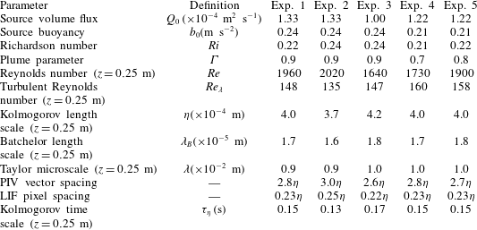
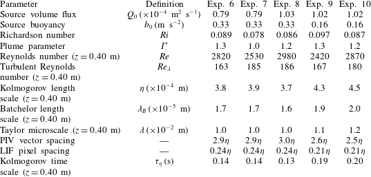
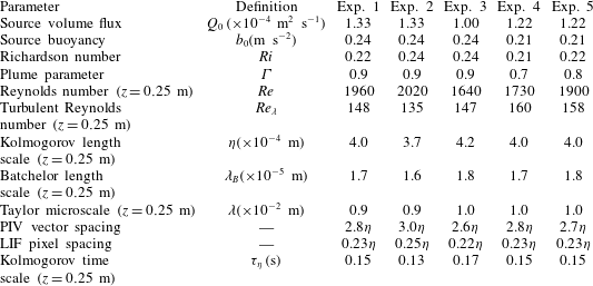
Experimental parameters and measured length and time scales of the free plume experiments. Definitions are provided in the text.
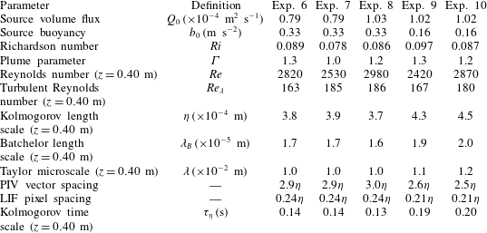
Experimental parameters and measured length and time scales of the wall plume experiments.
Measurements for the free plume were collected over a measurement window height of 0.160 m starting at a distance 0.165 m from the physical source of the free plume and a window height of 0.157 m starting at a distance 0.316 m from the physical source of the wall plume. These regions were sufficiently far from the source so that the plumes can be considered pure and self-similar. In order to minimise backflow effects the plumes were first run at relatively low flow rate. This ensured the resulting gravity current at the base of the tank had little effect on the ambient motion at the height of the measurement window. The flow rate was then gradually increased so that the higher momentum plumes entered a stratified region at the base of the tank which helped to mitigate the effects of the resulting gravity current. Each experiment was recorded for 100 s, corresponding to
 $10^{4}$
simultaneous velocity/density fields. We verified that the plumes satisfied the pure-plume criterion used by Paillat & Kaminski (Reference Paillat and Kaminski2014a
) of an invariant maximum velocity with height. In addition, we checked that the Richardson number was invariant with height. A total of 10 plumes were studied, five free plumes and five wall plumes, and the experimental source parameters are given in tables 2 and 3, respectively. Also given are the Reynolds number
 $Re=\overline{w}_{m}R/\unicode[STIX]{x1D708}$
at the mid height of the region examined, where
 $R$
is the plume half-width (free) and width (wall) defined in (2.9) and the plume parameter
 $\unicode[STIX]{x1D6E4}$
, averaged over the total height of the region examined, where
 $$\begin{eqnarray}\unicode[STIX]{x1D6E4}_{f}=\frac{Q_{f}^{3}F_{f}}{2\unicode[STIX]{x1D6FC}_{f}M_{f}^{3}}=\frac{Ri_{f}}{2\unicode[STIX]{x1D6FC}_{f}},\quad \unicode[STIX]{x1D6E4}_{w}=\frac{Q_{w}^{3}F_{w}}{\unicode[STIX]{x1D6FC}_{w}M_{w}^{3}}=\frac{Ri_{w}}{\unicode[STIX]{x1D6FC}_{w}}.\end{eqnarray}$$
We also calculate the turbulent Reynolds number,
 $Re_{\unicode[STIX]{x1D706}}=\overline{w^{\prime }}_{rms}\unicode[STIX]{x1D706}/\unicode[STIX]{x1D708}$
, the Kolmogorov length scale,
 $\unicode[STIX]{x1D702}=(\unicode[STIX]{x1D708}^{3}/\unicode[STIX]{x1D716})^{1/4}$
, the Taylor microscale,
 $\unicode[STIX]{x1D706}=\overline{w^{\prime }}_{rms}\sqrt{15\unicode[STIX]{x1D708}/\unicode[STIX]{x1D716}}$
, the Batchelor length scale,
 $\unicode[STIX]{x1D706}_{B}=\unicode[STIX]{x1D702}/Sc^{1/2}$
and the Kolmogorov time scale,
 $\unicode[STIX]{x1D70F}_{\unicode[STIX]{x1D702}}=\left(\unicode[STIX]{x1D708}/\unicode[STIX]{x1D716}\right)^{1/2}$
, where
 $\unicode[STIX]{x1D716}=15\unicode[STIX]{x1D708}\overline{(\unicode[STIX]{x2202}w/\unicode[STIX]{x2202}z)^{2}}$
and
 $Sc$
is the Schmidt number. The subscript
 $rms$
denotes the root mean square of the data. Tables 2 and 3 shows that the Batchelor length scale was much smaller than the resolution of the LIF images for all the experiments, suggesting that the effects of diffusion at these scales may be ignored in our analysis.
3.1.1 Detection of the TNTI
The TNTI of the plume and statistics conditional on the presence or absence of plume fluid were used to characterise the flow. Therefore, it was crucial that we were able to accurately detect and distinguish between ambient fluid and plume fluid. Given that the Batchelor length scale of the plumes was small compared to the resolution of the LIF measurements, we were able to employ a similar method to that used by Prasad & Sreenivasan (Reference Prasad and Sreenivasan1989) and Mistry et al. (Reference Mistry, Philip, Dawson and Marusic2016) to find the TNTI in an axisymmetric jet. We identified the TNTI by a scalar threshold,
 $b_{t}$
, which coincides with the inflection point of the area-averaged conditional mean buoyancy,
 $\widetilde{b}$
, and spanwise vorticity magnitude,
 $\widetilde{|\unicode[STIX]{x1D714}_{y}|}$
, where the conditional mean is an area-averaged quantity of regions where the buoyancy is measured above a given threshold,
 $b_{t}$
. The area-averaged conditional mean of the buoyancy and spanwise vorticity magnitude are defined as follows:
 $$\begin{eqnarray}\displaystyle & \displaystyle \widetilde{b}(b_{t})=\frac{\left.\displaystyle \iint \left(b(x,z)\,\text{d}x\,\text{d}z\right)\right|_{b>b_{t}}}{\left.\displaystyle \iint \,\text{d}x\,\text{d}z\right|_{b>b_{t}}}, & \displaystyle\end{eqnarray}$$
 $$\begin{eqnarray}\displaystyle & \displaystyle \widetilde{|\unicode[STIX]{x1D714}_{y}|}(b_{t})=\frac{\left.\displaystyle \iint \left(|\unicode[STIX]{x1D714}_{y}|(x,z)\,\text{d}x\,\text{d}z\right)\right|_{b>b_{t}}}{\left.\displaystyle \iint \,\text{d}x\,\text{d}z\right|_{b>b_{t}}}. & \displaystyle\end{eqnarray}$$
Mistry et al. (Reference Mistry, Philip, Dawson and Marusic2016) also consider the conditional mean vertical velocity in their identification of
 $b_{t}$
. However, given the finding that significant vertical velocities exist outside the scalar edge of an axisymmetric plume (Burridge et al.
Reference Burridge, Parker, Kruger, Partridge and Linden2017), we chose to consider instead only the buoyancy and spanwise vorticity magnitude, as the flow outside the plume is irrotational. The conditional buoyancy and spanwise vorticity magnitude, with their gradients, are shown in figure 3(a–d). For the wall plume an inflection point was identified from the conditionally averaged buoyancy and vorticity data with a value of
 $b_{t}/\overline{b}_{m}=0.15$
and
 $b_{t}/\overline{b}_{m}=0.17$
, respectively. Although these values do not coincide exactly, the inflection point of the conditionally averaged spanwise vorticity magnitude falls within
 $0.17\pm 20\,\%$
. We show in § 5 that our results are not sensitive to the choice of threshold within this range. For the free plume an inflection point was identified from the conditionally averaged buoyancy data with a value of
 $b_{t}/\overline{b}_{m}=0.35$
. An inflection point for the conditionally averaged vorticity data could not be identified, although as we show, this choice of threshold clearly identifies a region separating a significant jump in spanwise vorticity magnitude. In addition, in the following sections, we show that the results are insensitive to the choice of the threshold within a range of
 $0.35\pm 20\,\%$
.
Identification of the scalar threshold,
 $b_{t}$
, used to identify the TNTI of the (a) free and (b) wall plume. Panels (c) and (d) show the gradient of the conditionally averaged profiles of (a) and (b), respectively. The vertical dashed line shows the position of the inflection point of the conditionally averaged buoyancy data of the free plume,
 $b_{t}/\overline{b}_{m}=0.35$
, and wall plume,
 $b_{t}/\overline{b}_{m}=0.17$
.


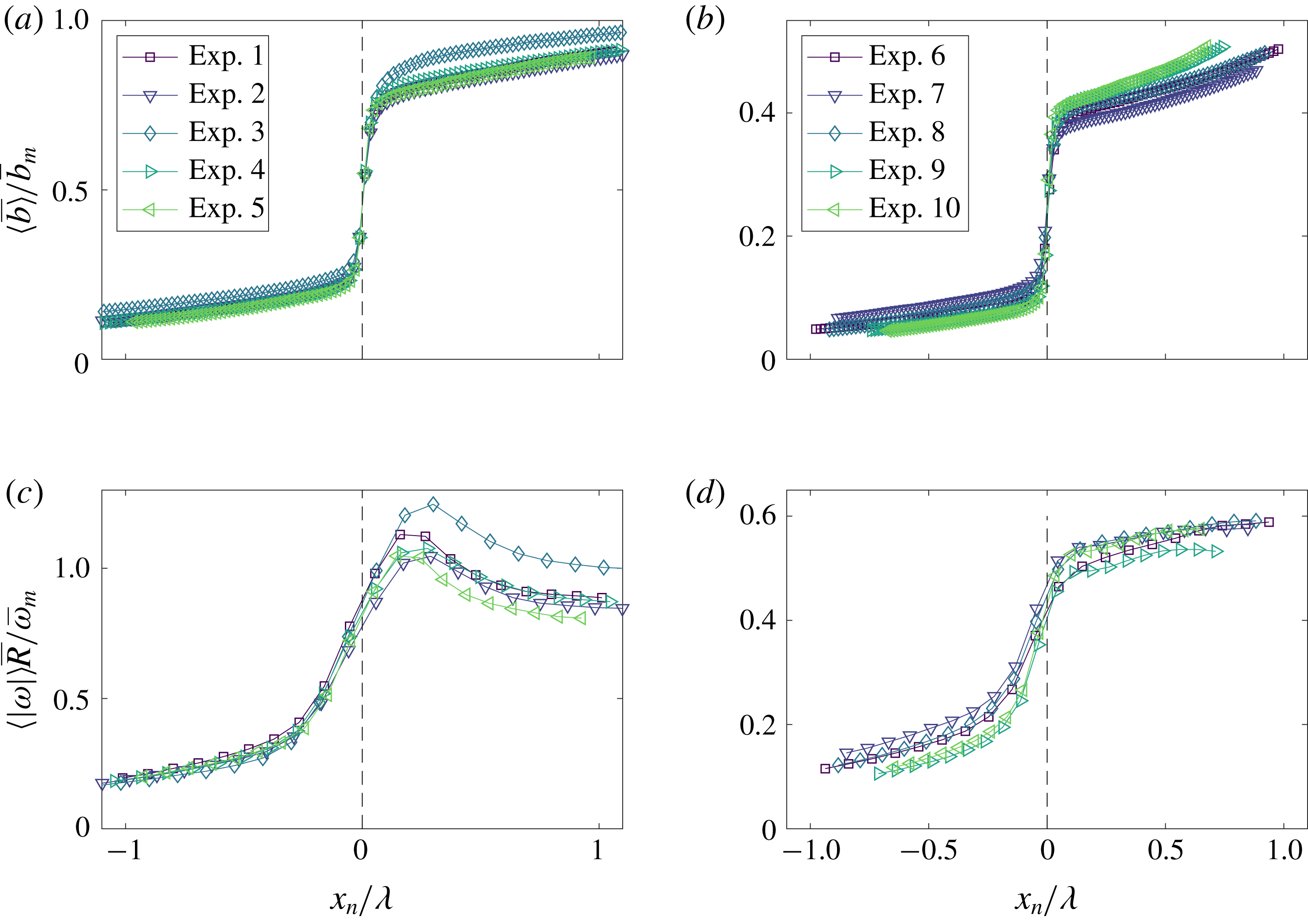
Figure 4 shows conditionally averaged profiles of buoyancy and spanwise vorticity magnitude, for both the free and wall plume. The data are ensemble averaged, represented by
 $\langle {\sim}\rangle$
, by a coordinate,
 $x_{n}$
, defined relative and normal to the TNTI, so that positive
 $x_{n}$
lies within the turbulent region of the plume (Chauhan et al.
Reference Chauhan, Philip, de Silva, Hutchins and Marusic2014; Mistry et al.
Reference Mistry, Philip, Dawson and Marusic2016; Mistry, Dawson & Kerstein Reference Mistry, Dawson and Kerstein2018). The TNTIs were identified using the threshold determined above. As noted by Mistry et al. (Reference Mistry, Philip, Dawson and Marusic2016), there may be multiple TNTI crossings along
 $x_{n}$
. Only regions that remain turbulent are included in the ensemble average of
 $x_{n}>0$
and vice versa. Figures 4(a) and (b) show there is a rapid increase in measured buoyancy across the identified TNTI,
 $x_{n}=0$
, in the free and wall plume, respectively. Analogous observations, where a passive scalar is measured, are also found in the near and far field of a turbulent jet (Westerweel et al.
Reference Westerweel, Fukushima, Pedersen and Hunt2009; Mistry et al.
Reference Mistry, Philip, Dawson and Marusic2016, Reference Mistry, Dawson and Kerstein2018). A jump in spanwise vorticity magnitude can also be observed in the free and wall plume in figures 4(c) and (d), respectively, which coincides with the jump in buoyancy at
 $x_{n}=0$
. As a result of the lower resolution of the velocity field data the relative increase in spanwise vorticity magnitude is not as sharp as that for the buoyancy (note that for measurements based on both the velocity and buoyancy field the jumps occur over approximately 4–5 data points). Furthermore, the spanwise vorticity magnitude jump occurs across a distance approximately equal to the Taylor microscale. This is consistent with the results of direct numerical simulations of a turbulent wake by Bisset, Hunt & Rogers (Reference Bisset, Hunt and Rogers2002), and the experimental results of a turbulent free line jet by Terashima et al. (Reference Terashima, Sakai, Nagata, Ito, Onishi and Shouji2016), where in both cases the TNTI thickness was found to be almost equal to the Taylor microscale. It is apparent from figures 4(a) and 4(b) as to why the threshold in the free plume is approximately double that of the wall plume. As will be discussed in § 6, the free plume is more uniformly mixed within the plume region resulting in larger buoyancy, relative to the maximum buoyancy, within the plume close to the interface. Given that the jump in relative buoyancy in the free plume is approximately double that of the wall plume, a larger threshold may be chosen to identify the region separating the ambient and plume fluid. From this analysis we are therefore confident that the threshold identified is robust in identifying the TNTI across all the experiments. We therefore choose
 $b_{t}/\overline{b}_{m}=0.17$
as the threshold of the wall plume and
 $b_{t}/\overline{b}_{m}=0.35$
as the threshold of the free plume throughout the study. We may now consider regions
 $b<b_{t}$
to be ambient fluid and regions
 $b>b_{t}$
to be plume fluid.
4 Validation of the PIV and LIF data
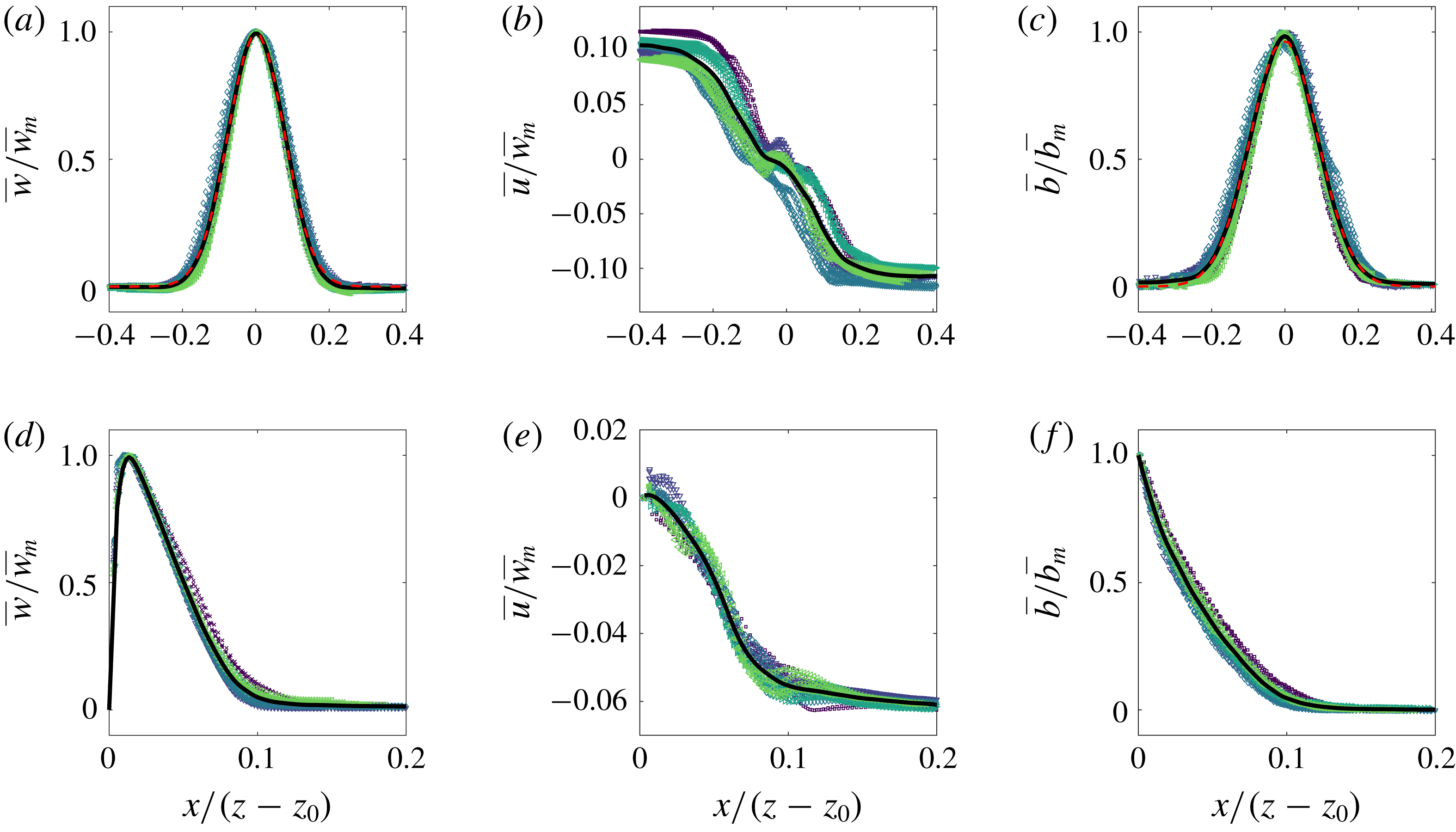
Time-averaged scaled vertical and horizontal velocity and buoyancy profiles of the (a–c) free and (d–f) wall plume. For each experiment, five different heights spanning the studied region are plotted. The average values across all experiments are shown in each case by the solid black curve. In addition, a Gaussian least-squares fit was performed on the average values of the vertical velocity and buoyancy of the free plume and are shown by the dashed red curves.
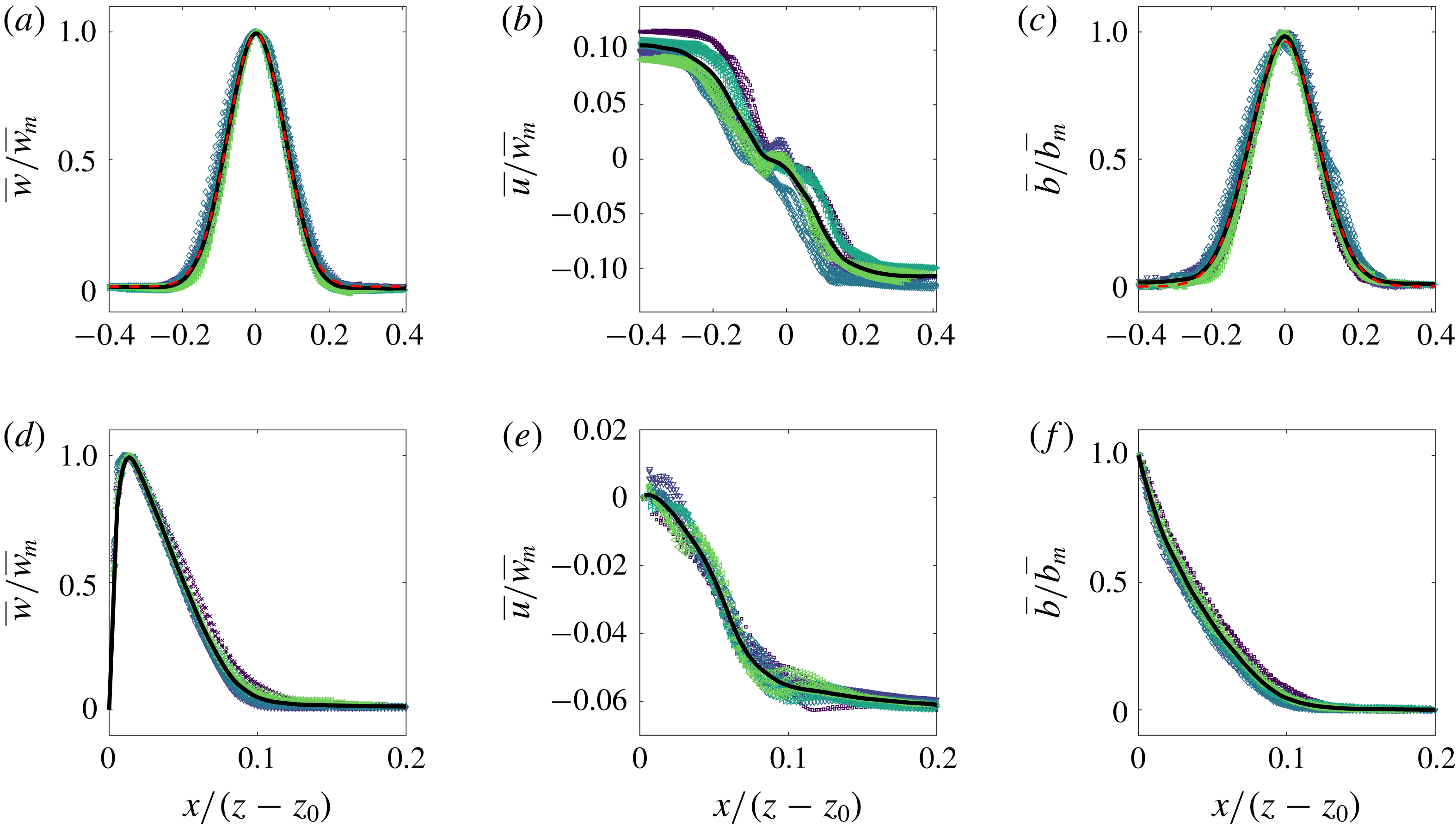
We first validate the plume data by demonstrating the self-similar behaviour of the velocity and buoyancy profiles. Figure 5 shows the vertical and horizontal velocities and buoyancy profiles at five different heights spanning the whole height of the measurement window for each experiment, with horizontal distances scaled on the distance from the virtual source,
 $z-z_{0}$
, where
 $z_{0}$
is the virtual origin. The virtual origin was calculated by identifying, by linear extrapolation, the vertical location at which the time-average plume width is zero. A good collapse of data on to a single curve is seen in each plot, thereby demonstrating self-similarity. The self-similar vertical velocity and buoyancy profiles of the free plume are fitted well by a Gaussian curve (shown by the dashed red curve) as has been previously observed (e.g. Ramaprian & Chandrasekhara Reference Ramaprian and Chandrasekhara1989; Paillat & Kaminski Reference Paillat and Kaminski2014a
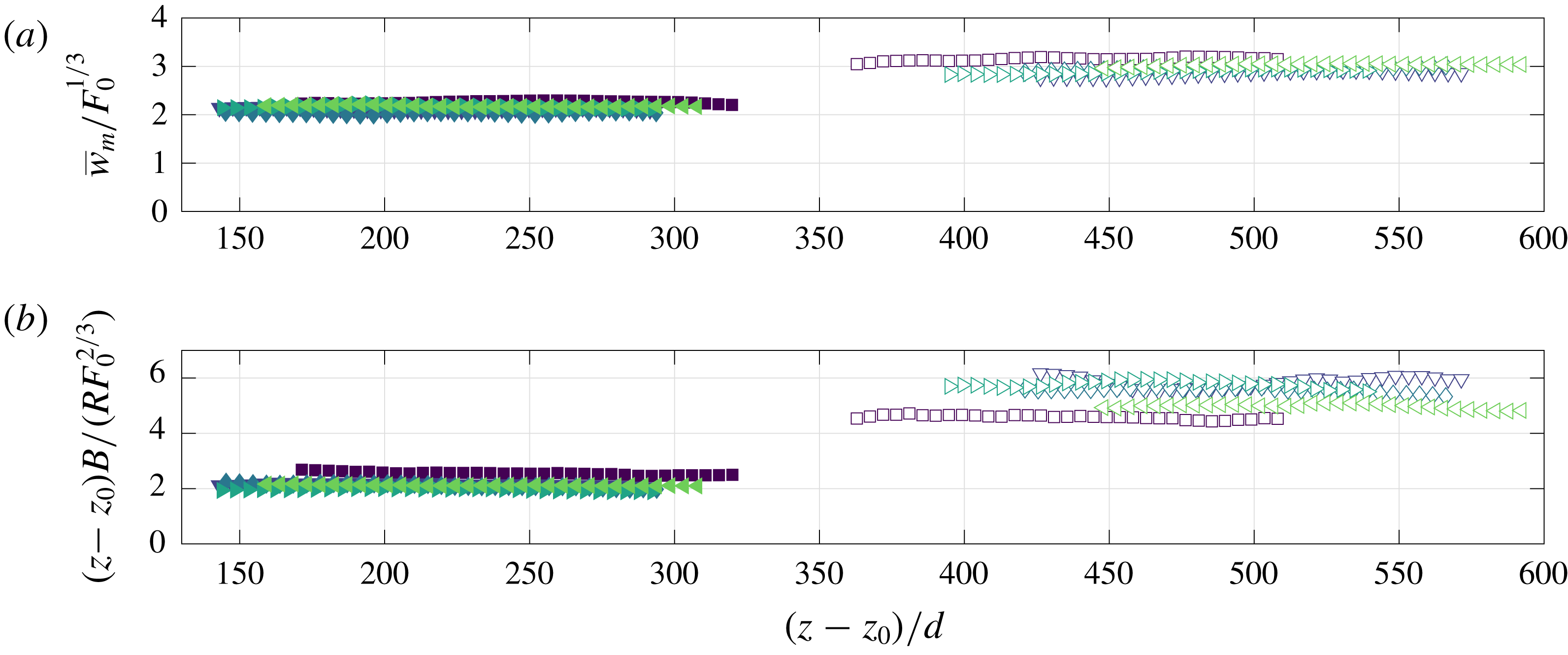
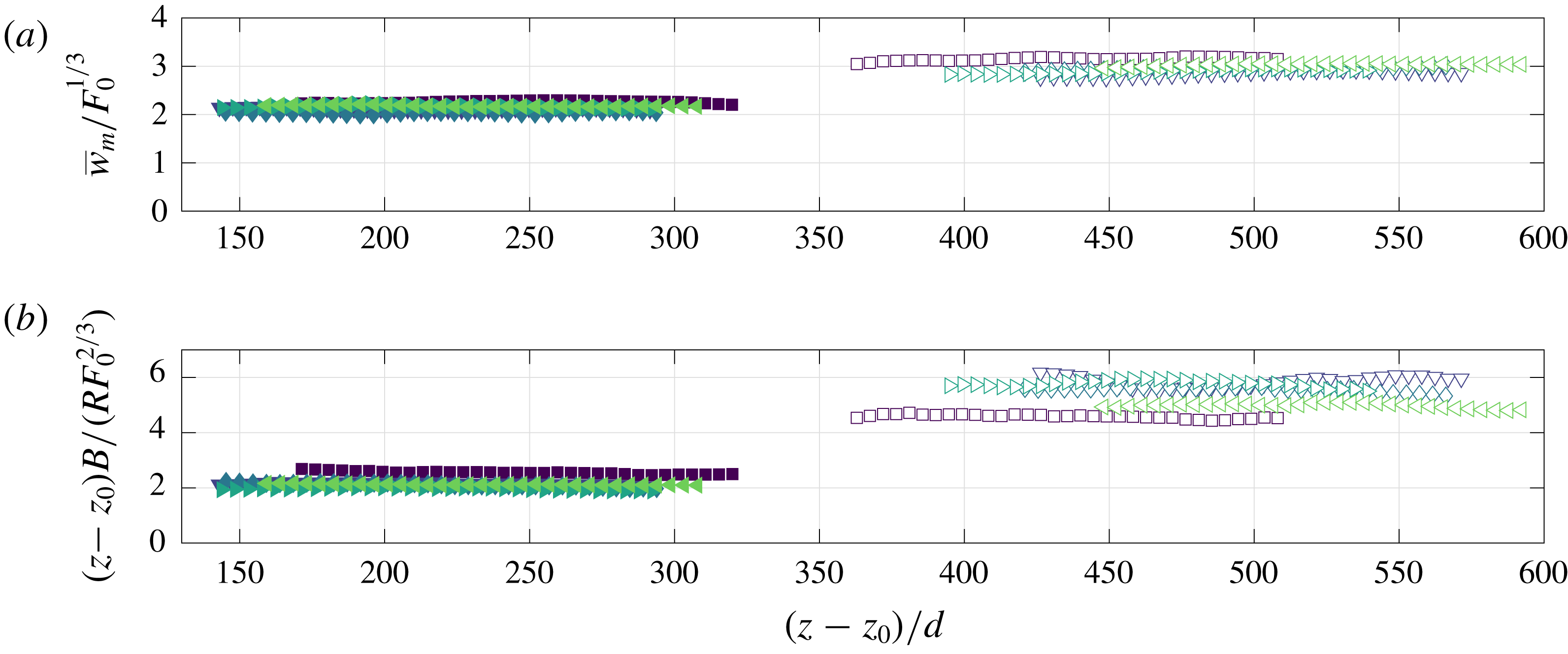
) and the wall plume profiles agree well with those of Sangras, Dai & Faeth (Reference Sangras, Dai and Faeth1999) and Sangras et al. (Reference Sangras, Dai and Faeth2000). Further confidence in the self-similarity of the plumes is given by the invariance with height of the maximum vertical velocity, scaled by the buoyancy flux
 $F_{0}^{1/3}$
, shown in figure 6(a), and the inverse linear decay
 ${\sim}1/z$
(Fischer et al.
Reference Fischer, List, Imberger, Koh and Brooks1979) of the top-hat buoyancy
 $B/R$
shown in the compensated plot in figure 6(b).
(a) Maximum vertical velocities of the free (filled markers) and wall plume (unfilled markers) scaled using the source buoyancy flux. (b) Time-averaged top-hat buoyancy of the free and wall plume, scaled using the vertical distance and source buoyancy flux.
5 Results in an Eulerian coordinate system
5.1 Entrainment coefficient
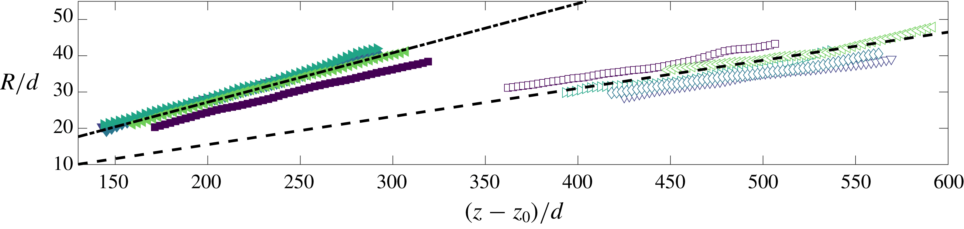
The variation in the mean free plume half-width (filled markers) and wall plume width (unfilled markers). Lines of best fit, used to calculate the entrainment values (table 4), are shown by the respective dashed lines.
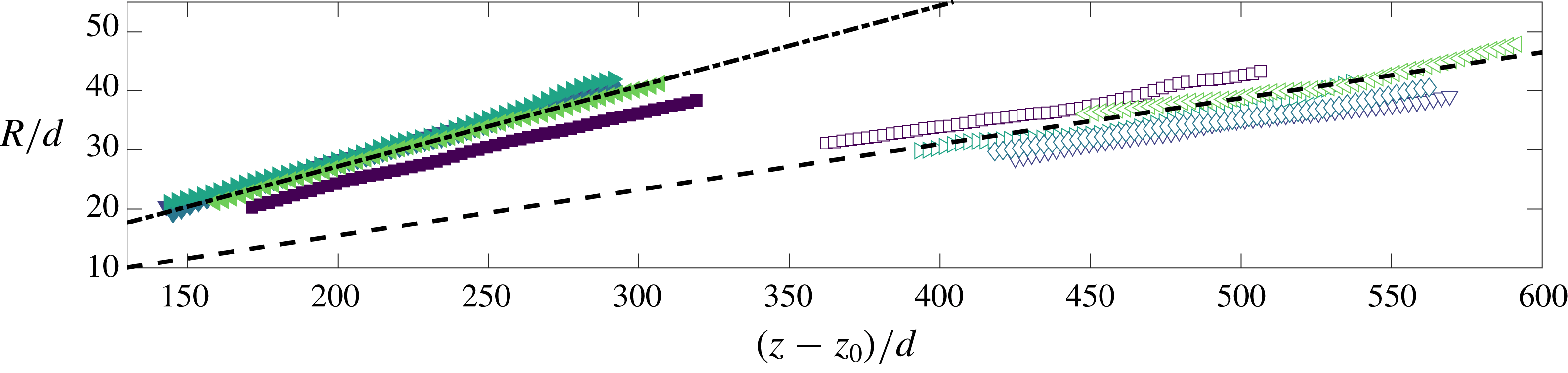
The top-hat entrainment coefficients for the free and wall plume were determined from the relation
 $\unicode[STIX]{x1D6FC}=\text{d}R/\text{d}z$
, which may be derived from the solutions of the conservation equations (2.14)–(2.16) and (2.20)–(2.22), respectively. The values were obtained from a least-squares best-fit to the plume widths,
 $R$
, at each height (figure 7). The calculated values are shown in table 4 where the tolerances indicate the standard deviation in the values measured across the five independent experiments examined for each flow. Our value of
 $\unicode[STIX]{x1D6FC}_{f}$
is consistent with previously reported Gaussian entrainment values of
 $\unicode[STIX]{x1D6FC}_{f,G}=\{0.10,0.16\}$
which correspond to approximately
 $\unicode[STIX]{x1D6FC}_{f}\approx \sqrt{2}\unicode[STIX]{x1D6FC}_{f,G}=\{0.14,0.22\}$
. Our value of
 $\unicode[STIX]{x1D6FC}_{w}$
is lower than the previously reported value of
 $\unicode[STIX]{x1D6FC}_{w}=0.095\pm 0.005$
in Grella & Faeth (Reference Grella and Faeth1975). In particular, our results support previous studies that find
 $\unicode[STIX]{x1D6FC}_{w}$
is slightly more than half of
 $\unicode[STIX]{x1D6FC}_{f}$
. We note that if we were to consider the wall plume as ‘half’ the free plume, we would expect the top-hat entrainment values to be equal to one another since the equation expressing conservation of volume flux in the free plume (2.11) accounts for the double-sided entrainment with the factor of
 $2$
. Consequently, this difference is a result of the absence or presence of the wall.


We also calculate the entrainment coefficient based on the decomposition outlined in § 2.1. The relative contributions of
 $\unicode[STIX]{x1D6FC}_{production}$
and
 $\unicode[STIX]{x1D6FC}_{buoyant}$
, and their sum, are shown in table 4 compared to the entrainment coefficient calculated directly from
 $\text{d}R/\text{d}z$
.
There is good agreement between the calculated entrainment coefficients of the free plume between the two methods. Our values of
 $\unicode[STIX]{x1D6FC}_{production}$
and
 $\unicode[STIX]{x1D6FC}_{buoyancy}$
are in good agreement with that measured by Paillat & Kaminski (Reference Paillat and Kaminski2014a
), where they find that
 $\unicode[STIX]{x1D6FC}_{production}=0.104$
, and
 $\unicode[STIX]{x1D6FC}_{buoyant}=0.04$
, where the latter has been inferred from the Richardson number given in Paillat & Kaminski (Reference Paillat and Kaminski2014a
) of
 $Ri=0.14$
.
The terms
 $\unicode[STIX]{x1D6FC}_{production}$
and
 $\unicode[STIX]{x1D6FC}_{buoyant}$
for the wall plume may be accurately determined from our data. However, the component
 $\unicode[STIX]{x1D6FC}_{viscous}$
for the wall plume is difficult to measure directly. Given that such good agreement is found in the free plume, it is suggestive that the discrepancy between
 $\unicode[STIX]{x1D6FC}_{f}$
and the turbulent production and buoyant terms,
 $\unicode[STIX]{x1D6FC}_{production}$
and
 $\unicode[STIX]{x1D6FC}_{buoyant}$
, may be attributed to the viscous term,
 $\unicode[STIX]{x1D6FC}_{viscous}$
, since the discrepancy lies outside the range of error values calculated. We therefore estimate that for the wall plume
 $\unicode[STIX]{x1D6FC}_{viscous}\approx -0.03$
.
The contribution from the buoyancy,
 $\unicode[STIX]{x1D6FC}_{buoyant}$
, is approximately the same in both the free and wall plume. The reduction in entrainment in the wall plume may then be attributed to both a significant reduction in turbulent production,
 $\unicode[STIX]{x1D6FC}_{production}$
, and viscous dissipation in the inner layer,
 $\unicode[STIX]{x1D6FC}_{viscous}$
. The reduction in
 $\unicode[STIX]{x1D6FC}_{production}$
between the free and wall plume is approximately equal to
 $\unicode[STIX]{x1D6FC}_{viscous}$
in the wall plume, which shows that both contribute significantly to reducing entrainment.
5.2 Entrainment flux
The entrainment coefficient may be viewed as a measure of the plume entrainment efficiency. However, to interpret the physical implications we consider how much fluid is entrained into the free and wall plume per unit height. For a given buoyancy flux
 $F=F_{w}=F_{f}$
, equations (2.14) and (2.20) give
 $$\begin{eqnarray}\frac{2u_{\infty ,f}}{u_{\infty ,w}}=\frac{\text{d}Q_{f}}{\text{d}z}\left(\frac{\text{d}Q_{w}}{\text{d}z}\right)^{-1}=2^{2/3}\left(\frac{\unicode[STIX]{x1D6FC}_{f}}{\unicode[STIX]{x1D6FC}_{w}}\right)^{2/3}\left(1+\frac{C}{\unicode[STIX]{x1D6FC}_{w}}\right)^{1/3},\end{eqnarray}$$
where we have used that
 $(\unicode[STIX]{x1D703}_{f}/\unicode[STIX]{x1D703}_{w})^{1/3}\approx 1$
, as verified from our data.
The coefficient of friction
 $C$
was found from balancing bulk flow quantities using the momentum equation (2.18), with a value of
 $C=0.015\pm 0.005$
being determined. We note the difficulties in experimentally determining this value due to the omission of the vertical velocity fluctuations and pressure term (the latter of which cannot be measured directly) in the vertical momentum equation, which together have been shown to account for up to
 $8\,\%$
of the mean vertical momentum in an axisymmetric plume (van Reeuwijk et al.
Reference van Reeuwijk, Salizzoni, Hunt and Craske2016). Therefore, we do not place emphasis on our result of the skin friction coefficient, and note that our conclusions are qualitatively the same for any (reasonable) values of
 $C\geqslant 0$
.
Using the determined entrainment values in the right-hand side of (5.1) we find that
 $2u_{\infty ,f}/u_{\infty ,w}=2.5\pm 0.4$
. This agrees with direct measurements of
 $(\text{d}Q_{f}/\text{d}z)/(\text{d}Q_{w}/\text{d}z)=2.4\pm 0.1$
. Hence, despite the value of the entrainment coefficient for a free plume being less than double that of the wall plume, the increase in volume flux with height in a free plume is significantly greater than double that of a wall plume with equal forcing i.e. equivalent buoyancy flux. This implies that each edge of the free plume entrains ambient fluid more efficiently than the wall plume, per unit height.
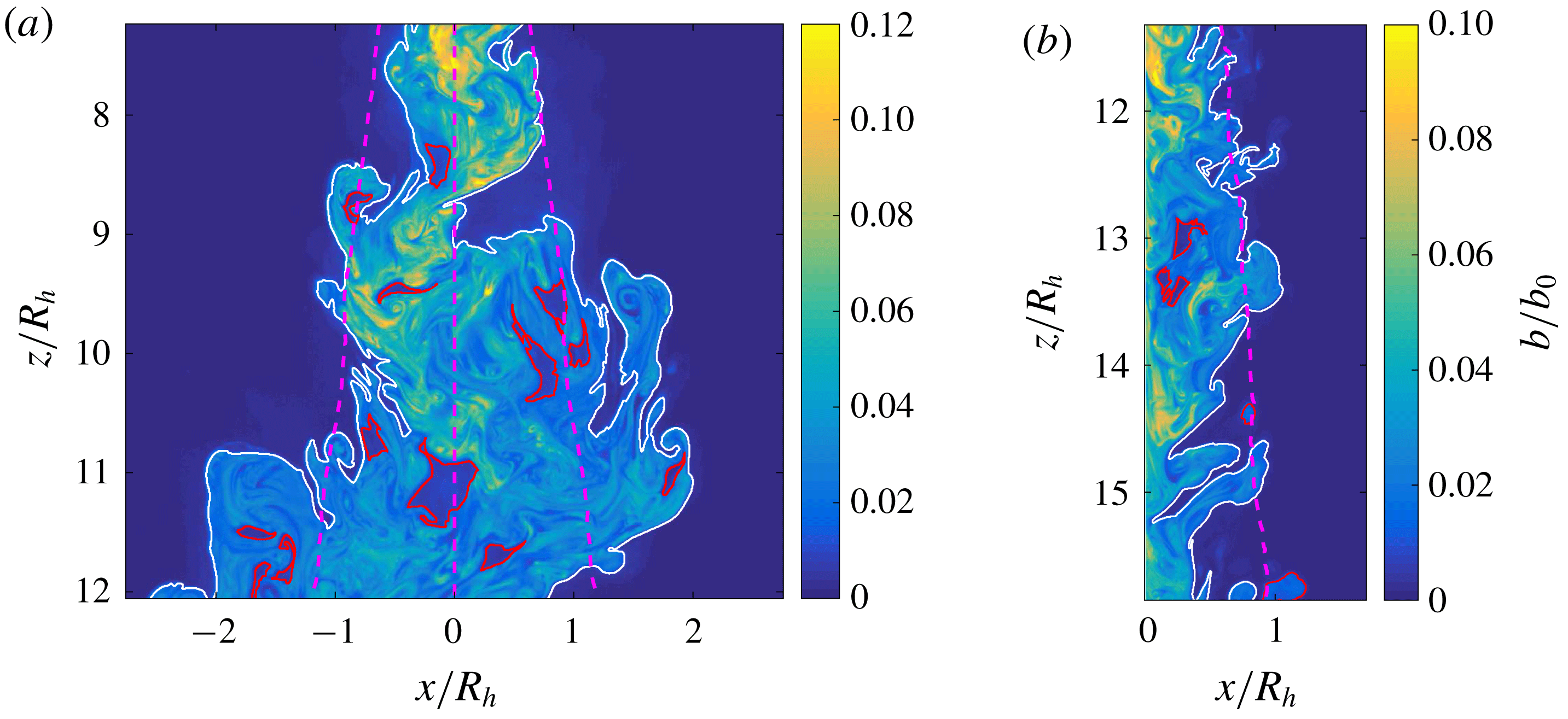
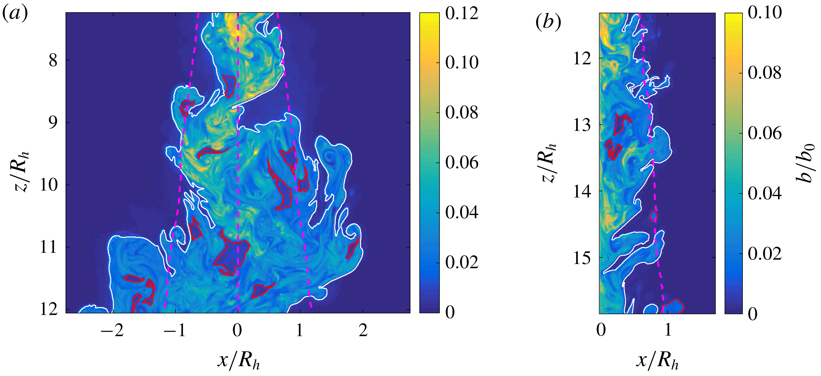
Instantaneous buoyancy field of the (a) free and (b) wall plume. The figures shown are the processed LIF images at full resolution. In both cases the outer continuous TNTI is highlighted by the solid white line and the TNTIs of unconnected regions and completely engulfed ambient fluid are highlighted by the red lines. The TNTIs were identified from the threshold determined in § 3.1.1. In (a) the mean position of the outer left TNTI, centreline and outer right TNTI are denoted by the dashed magenta lines from left to right and the distances have been scaled using the free plume half-width at the mid height of the image,
 $R_{h}$
. In (b) the position of the mean outer TNTI of the free plume is denoted by the dashed magenta line and the distances have been scaled using the wall plume width at the mid height of the image,
 $R_{h}$
.
5.3 The statistics of the TNTI
Figure 8 shows instantaneous images of a free and a wall plume. The continuous outer TNTI has been identified and highlighted in white. Also highlighted, in red, are the TNTIs of regions of unmixed ambient fluid completely engulfed, within the plane, by plume fluid. In both flows, there are significant deviations from the positions of the mean outer TNTI, denoted by the dashed magenta lines. The meandering nature of the free plume is evident from figure 8(a), where in addition to the relatively small coherent structures forming, i.e. eddies along the outer TNTI, which are also seen in the wall plume, the free plume also forms coherent structures at the length scale of the full plume width. As a result the instantaneous edge of the wall plume is comparatively closer to the mean TNTI (figure 8 b) than for the free plume.
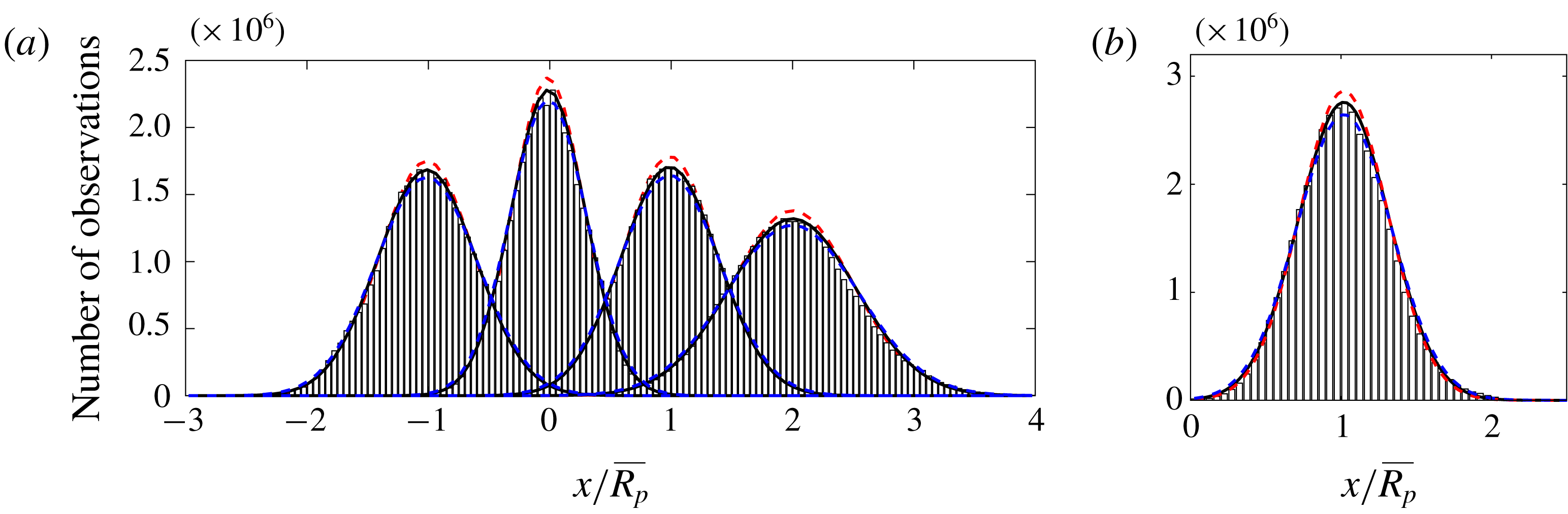
Histograms of (a) the locations (from left to right) of the left-TNTI, the centre, the right-TNTI and the plume scalar width of the free plume, where distances are normalised by the plume scalar half-width and (b) the plume scalar width of the wall plume normalised by the time-average scalar width,
 $\overline{R_{p}}$
. The solid curves are Gaussian best fits to the data. The red and blue dashed curves show the Gaussian best fits to data of the statistics performed with a threshold of
 $b_{t}/b_{m}=0.17-20\,\%$
and
 $b_{t}/b_{m}=0.17+20\,\%$
, respectively, for the wall plume and
 $b_{t}/b_{m}=0.35-20\,\%$
and
 $b_{t}/b_{m}=0.35+20\,\%$
, respectively, for the free plume, highlighting the insensitivity of our results to the choice of threshold.

We define the left,
 $E_{L}(z,t)$
, and right,
 $E_{R}(z,t)$
, points along the outermost TNTI for a given height and time, as the outermost left and right points along that TNTI at that height. Therefore, the positions are uniquely defined for each height and time. Similarly, we define the outermost point, at a given height and time, of the wall plume
 $R_{p}(z,t)$
. Histograms of
 $E_{L}(z,t)$
and
 $E_{R}(z,t)$
of the free plume and
 $R_{p}(z,t)$
of the wall plume are shown in figure 9, normalised by the time-averaged scalar widths of the plumes. We define the instantaneous plume scalar half-width and centreline as,
 $R_{p}=(E_{R}-E_{L})/2$
, and,
 $C_{P}=(E_{R}+E_{L})/2$
, respectively for the free plume and the scalar width as the distance from the wall to the outer TNTI in the wall plume. We find that the positions of the left and right TNTI of the free plume are both well represented by Gaussian distributions
 $E_{L}\sim N(\unicode[STIX]{x1D707}=-1,\unicode[STIX]{x1D70E}^{2}=0.16)$
,
 $E_{R}\sim N(\unicode[STIX]{x1D707}=1,\unicode[STIX]{x1D70E}^{2}=0.16)$
, respectively, where
 $\unicode[STIX]{x1D707}$
denotes the mean and
 $\unicode[STIX]{x1D70E}$
the standard deviation. The sensitivity of the results to the particular choice of threshold were tested, for
 $b_{t}/\overline{b}_{m}=0.35\pm 20\,\%$
, also shown in figure 9, in each case the standard deviation varied by at most
 $5\,\%$
as compared to the standard deviation of the chosen threshold. The free plume scalar half-width and centreline are also approximated by Gaussian distributions,
 $2R_{p}\sim N(\unicode[STIX]{x1D707}=2,\unicode[STIX]{x1D70E}^{2}=0.27)$
,
 $C_{P}\sim N(\unicode[STIX]{x1D707}=0,\unicode[STIX]{x1D70E}^{2}=0.093)$
. For the wall plume we find that
 $R_{p}\sim N(\unicode[STIX]{x1D707}=1,\unicode[STIX]{x1D70E}^{2}=0.091)$
, again the sensitivity of the results to the particular choice of threshold was tested, for
 $b_{t}/\overline{b}_{m}=0.17\pm 20\,\%$
, also shown in figure 9, in each case the standard deviation,
 $\unicode[STIX]{x1D70E}$
, varied by at most
 $4\,\%$
as compared to the standard deviation of the chosen threshold. In the case of the free plume, since
 $C_{P}=(E_{R}+E_{L})/2$
, it follows that the Pearson’s correlation coefficient is
 $\unicode[STIX]{x1D70C}_{E_{R},E_{L}}=0.16$
. This may be compared to a free axisymmetric plume where it was found that
 $\unicode[STIX]{x1D70C}_{E_{R},E_{L}}=0$
(Burridge et al.
Reference Burridge, Parker, Kruger, Partridge and Linden2017). So although the correlation between the two edges is larger than that for an axisymmetric plume, it is still small.
However, this statistic masks the true meandering nature of the plume as is evident from figure 8(a). The positions of the outer left and right TNTI of the free plume at, say,
 $z/R=9.0$
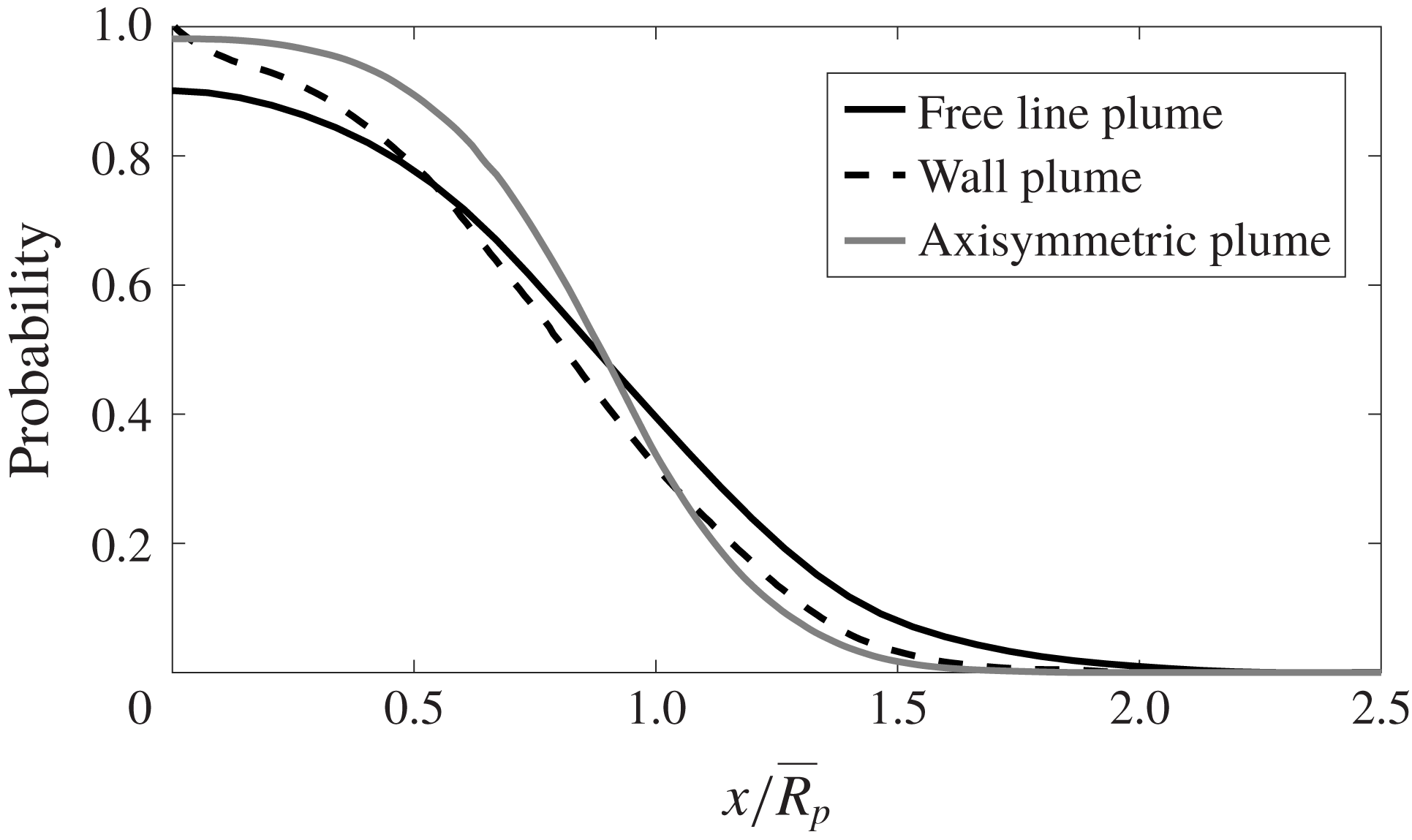
do not demonstrate meandering, even though the body of the plume has clearly meandered to the left and overturned. For this reason, the meandering nature of the plume is more robustly demonstrated by considering the probability, at a given horizontal location, of plume fluid being within the connected region that is bounded by the outer plume TNTI, as shown in figure 10. This demonstrates that, as a result of the plume meandering, there is a significant probability
 ${\sim}$
15 % that a connected region of ambient fluid exists at the mean centreline of the plume. For comparison, the equivalent probability function for an axisymmetric plume, which does not demonstrate a pronounced meandering behaviour, is shown (Burridge et al.
Reference Burridge, Parker, Kruger, Partridge and Linden2017) and the probability is much lower
 ${\sim}$
1 %. Kotsovinos (Reference Kotsovinos1975) and Westerweel et al. (Reference Westerweel, Fukushima, Pedersen and Hunt2005) have performed similar statistics for a free line and axisymmetric jet, respectively, and also find that there is a finite but very low probability of ambient fluid existing at the mean centreline. We note that Kotsovinos (Reference Kotsovinos1975) also calculated the plume fluid intermittency for a free line plume, and found it was almost identical to that of the free jet, which appears to be inconsistent with their observation of plume meandering.
The probability, at a given horizontal location, of being within the plume region bounded by the outer TNTI for the free plume (solid black line) wall plume (dashed black line) and for comparison an axisymmetric plume (grey line) (Burridge et al. Reference Burridge, Parker, Kruger, Partridge and Linden2017).

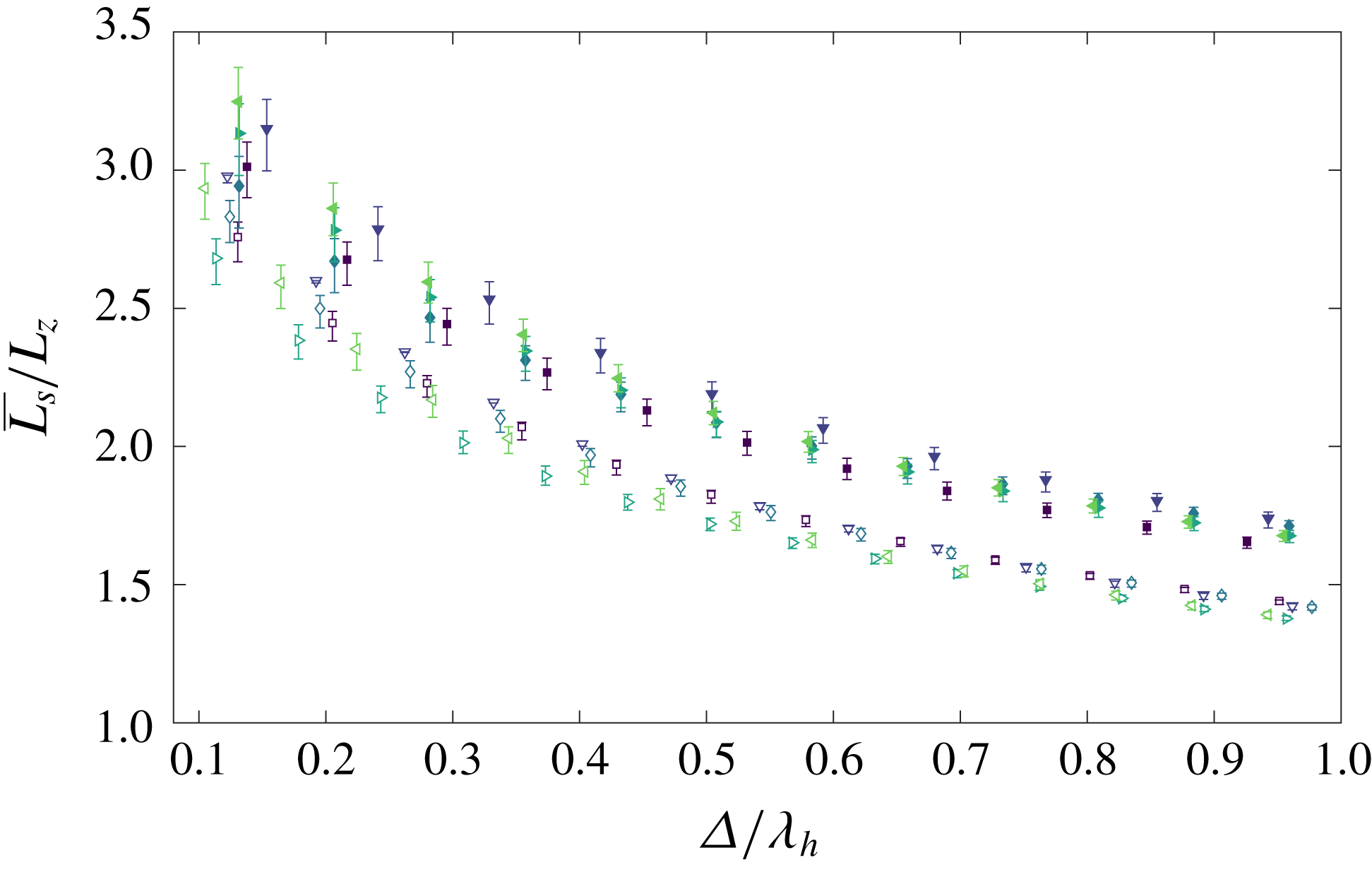
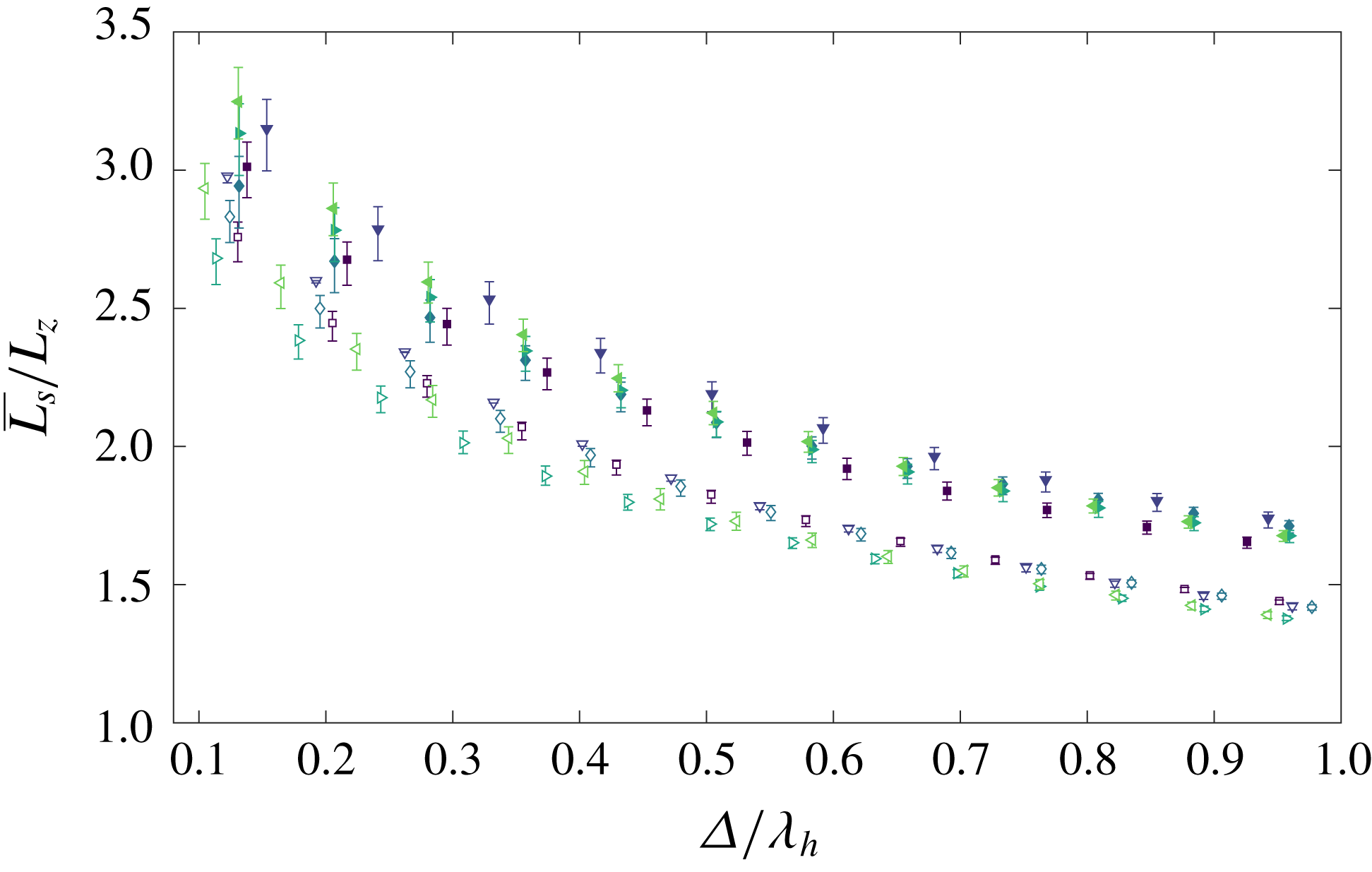
The mean TNTI length for varying box filter sizes,
 $0.1\leqslant \unicode[STIX]{x1D6E5}/\unicode[STIX]{x1D706}_{h}\leqslant 1$
, for the free (filled markers) and wall (unfilled markers) plume. The lengths have been scaled by the projected length of the interface. The error bars show the statistics performed with a threshold of
 $b_{t}/b_{m}=0.35\pm 20\,\%$
and
 $b_{t}/b_{m}=0.17\pm 20\,\%$
for the free and wall plumes, respectively.
The effect of the meandering can be quantified by considering the length of the TNTI of the free and wall plume. We use a methodology similar to that of Mistry et al. (Reference Mistry, Dawson and Kerstein2018), where box filtering of size
 $\unicode[STIX]{x1D6E5}$
is applied to each instantaneous image, and the TNTI is identified from the scalar threshold
 $b_{t}$
. Figure 8 shows an instantaneous buoyancy image at full resolution of the free and wall plume highlighting the identified TNTI. Completely engulfed and unconnected regions are included in the calculation which are non-negligible in the flows we are considering. The results for varying box sizes,
 $0.1<\unicode[STIX]{x1D6E5}/\unicode[STIX]{x1D706}_{h}<1$
, are shown in figure 11, where
 $\unicode[STIX]{x1D706}_{h}$
is the Taylor microscale measured at the mid height of the studied regions of the respective data and
 $0.1\unicode[STIX]{x1D706}_{h}$
approximately corresponds to the thickness of the light sheet used in the experiments. The mean interface length,
 $\overline{L_{s}}$
, is normalised by the projected interface length,
 $L_{z}$
, which is defined by the vertical distance of the region considered in the wall plume and twice the vertical distance in the free plume.
We find that the mean length of the TNTI of the free plume is larger than that of the wall plume at all filter sizes measured by a factor, on average, of at least
 $2.2$
. The sensitivity of the results to the particular choice of thresholds were tested for
 $b_{t}/\overline{b}_{m}=0.35\pm 20\,\%$
and
 $b_{t}/\overline{b}_{m}=0.17\pm 20\,\%$
for the free and wall plume, respectively. These data are shown by the error bars in figure 11. Although there is some sensitivity to the results the conclusion that
 $\overline{L_{s}}/L_{z}$
is larger in the free plume remains unchanged. The data does not exhibit any dependence on the turbulent Reynolds number which may be because of the limited range of turbulent Reynolds numbers across the experiments. In addition, the free and wall plume turbulent Reynolds numbers are similar, in particular experiments
 $4$
and
 $5$
of the free plume and experiments
 $6$
and
 $9$
of the wall plume where the turbulent Reynolds number at the mid height of the plumes differ by at most
 $6\,\%$
. Mistry et al. (Reference Mistry, Philip, Dawson and Marusic2016) found a similar value for the length of the TNTI of an axisymmetric jet, measured at
 $\unicode[STIX]{x1D6E5}/\unicode[STIX]{x1D706}_{h}\approx 1$
, to our measurements of the free plume of
 $\overline{L_{s}}/L_{z}\approx 2$
.
5.4 Conditional vertical transport
In order to quantify the effect of the meandering of the free plume on the large-scale engulfment we calculate the conditional vertical transport of ambient fluid, for both the free and wall plumes, by considering, separately, ambient fluid outside the TNTI envelope and engulfed but unmixed fluid. In order to calculate the fluxes of the ambient fluid we follow a method equivalent to that of Burridge et al. (Reference Burridge, Parker, Kruger, Partridge and Linden2017) by first defining an instantaneous step function for the outer ambient fluid
 $$\begin{eqnarray}H_{out}=\left\{\begin{array}{@{}ll@{}}0\quad & \text{ for }E_{L}(z,t)<x<E_{R}(z,t),\\ 1\quad & \text{ otherwise},\end{array}\right.\end{eqnarray}$$
and a step function for all unmixed fluid
 $$\begin{eqnarray}H_{amb}=\left\{\begin{array}{@{}ll@{}}0\quad & \text{ for }b(x,z,t)>b_{t}(z),\\ 1\quad & \text{ for }b(x,z,t)<b_{t}(z).\end{array}\right.\end{eqnarray}$$
A step function identifying the locations of engulfed but unmixed fluid
 $H_{eng}$
is then given by
 $H_{eng}=H_{amb}[1-H_{out}]$
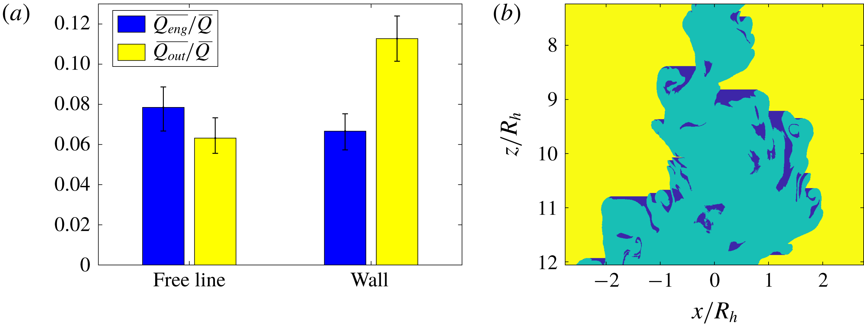
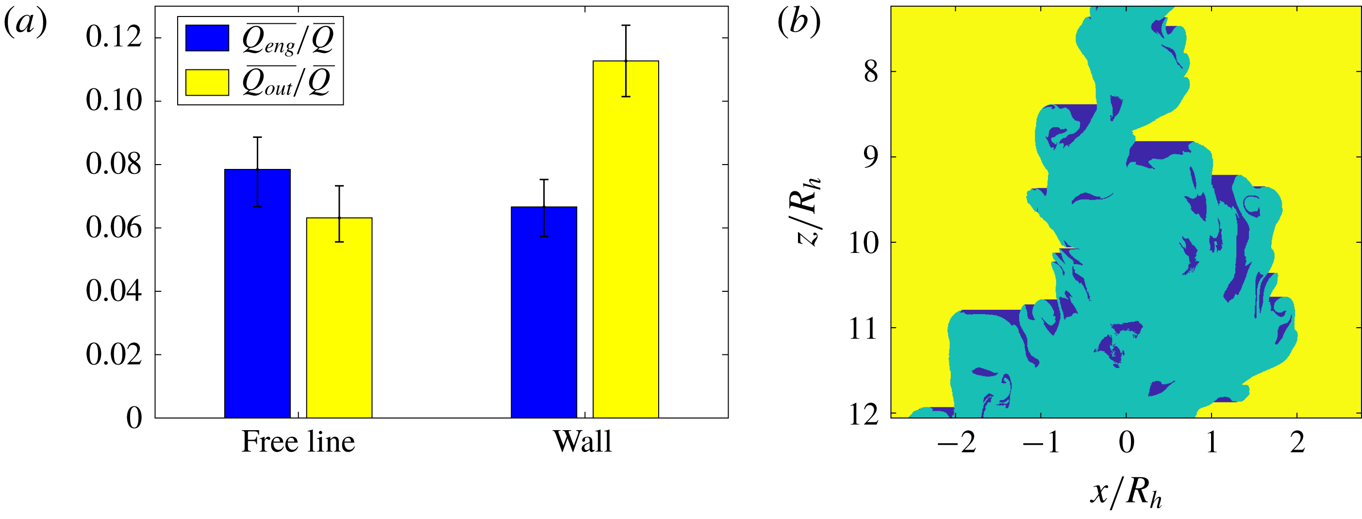
. Figure 12(b) shows an example of these regions for an instantaneous free plume image, where
 $H_{out}$
and
 $H_{eng}$
are highlighted in yellow and blue, respectively. The time-averaged volume flux of ambient fluid outside the plume TNTI envelope is then given by
 $$\begin{eqnarray}\overline{Q_{out}}(z)=\frac{1}{T}\int _{0}^{T}\int H_{out}(x,z,t)w(x,z,t)\,\text{d}x\,\text{d}t,\end{eqnarray}$$
where the integral domains over the
 $x$
-coordinate are given by the respective domains of the free plume
 $(-\infty ,\infty )$
and wall plume
 $(0,\infty )$
. Similarly, the time-averaged volume flux of engulfed but unmixed fluid is given by
 $$\begin{eqnarray}\overline{Q_{eng}}(z)=\frac{1}{T}\int _{0}^{T}\int H_{eng}(x,z,t)w(x,z,t)\,\text{d}x\,\text{d}t.\end{eqnarray}$$
Time-averaged results for both the free and wall plume are shown in figure 12(a). We find that for the free plume
 $\overline{Q_{eng}}/\overline{Q}=0.078\pm 0.011$
and
 $\overline{Q_{out}}/\overline{Q}=0.063\pm 0.011$
and for the wall plume
 $\overline{Q_{eng}}/\overline{Q}=0.067\pm 0.007$
and
 $\overline{Q_{out}}/\overline{Q}=0.113\pm 0.011$
. Again we see that more ambient fluid is engulfed by the meandering of the free plume compared with the wall plume.
(a) Time-averaged conditional volume flux of the ambient fluid outside the plume envelope (yellow) and of engulfed but unmixed ambient fluid (blue) for both the free and wall plume. The error bars indicate the mean values across the experiments of the analysis performed with a threshold of
 $b_{t}/b_{m}=0.35\pm 20\,\%$
and
 $b_{t}/b_{m}=0.17\pm 20\,\%$
for the free and wall plume, respectively. (b) Instantaneous image of a free plume, shown in figure 8(a), highlighting the different regions of ambient and engulfed fluid where the colours correspond to the bar plots in (a).
5.5 Turbulent fluxes
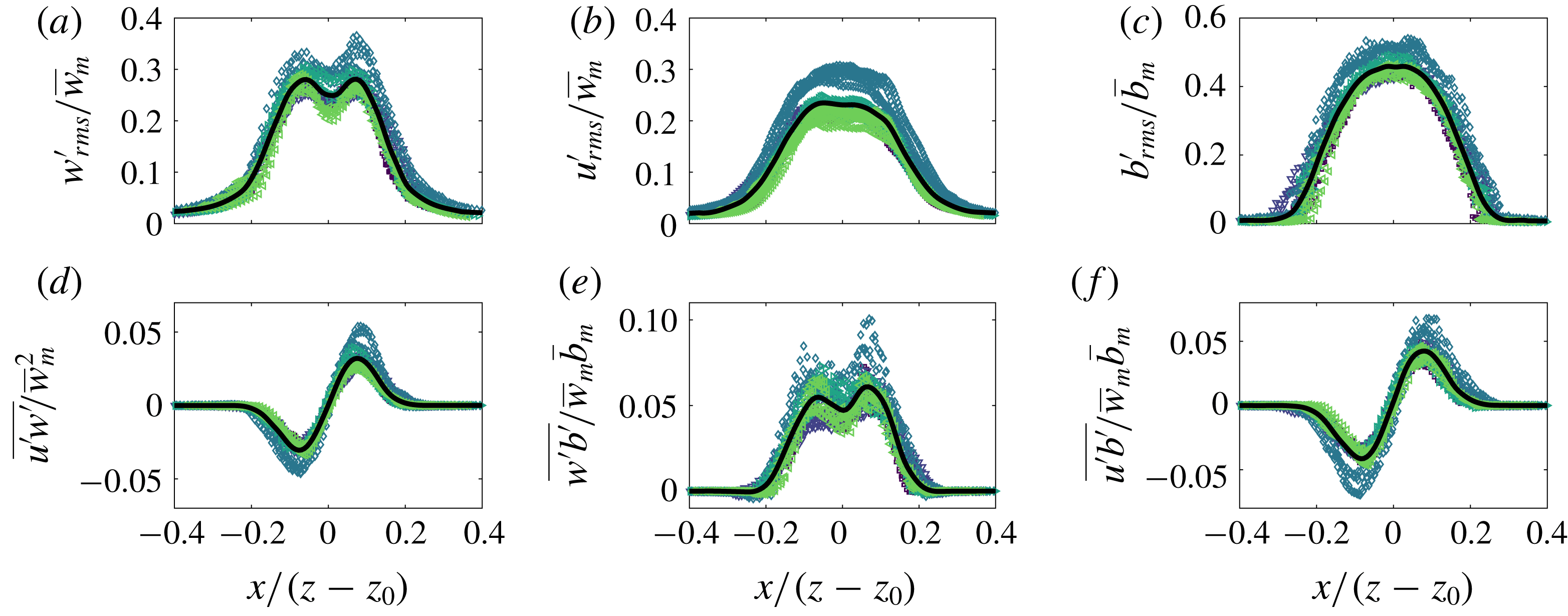
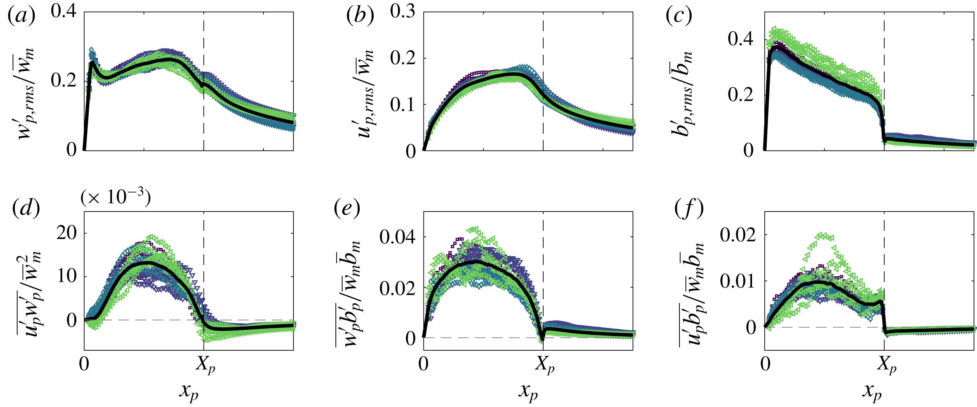
Time-averaged scaled free plume turbulent fluctuations of (a) vertical velocity, (b) horizontal velocity, (c) buoyancy, (d) Reynolds stress, (e) vertical and (f) horizontal turbulent buoyancy flux. The black curves are the averages of the data.

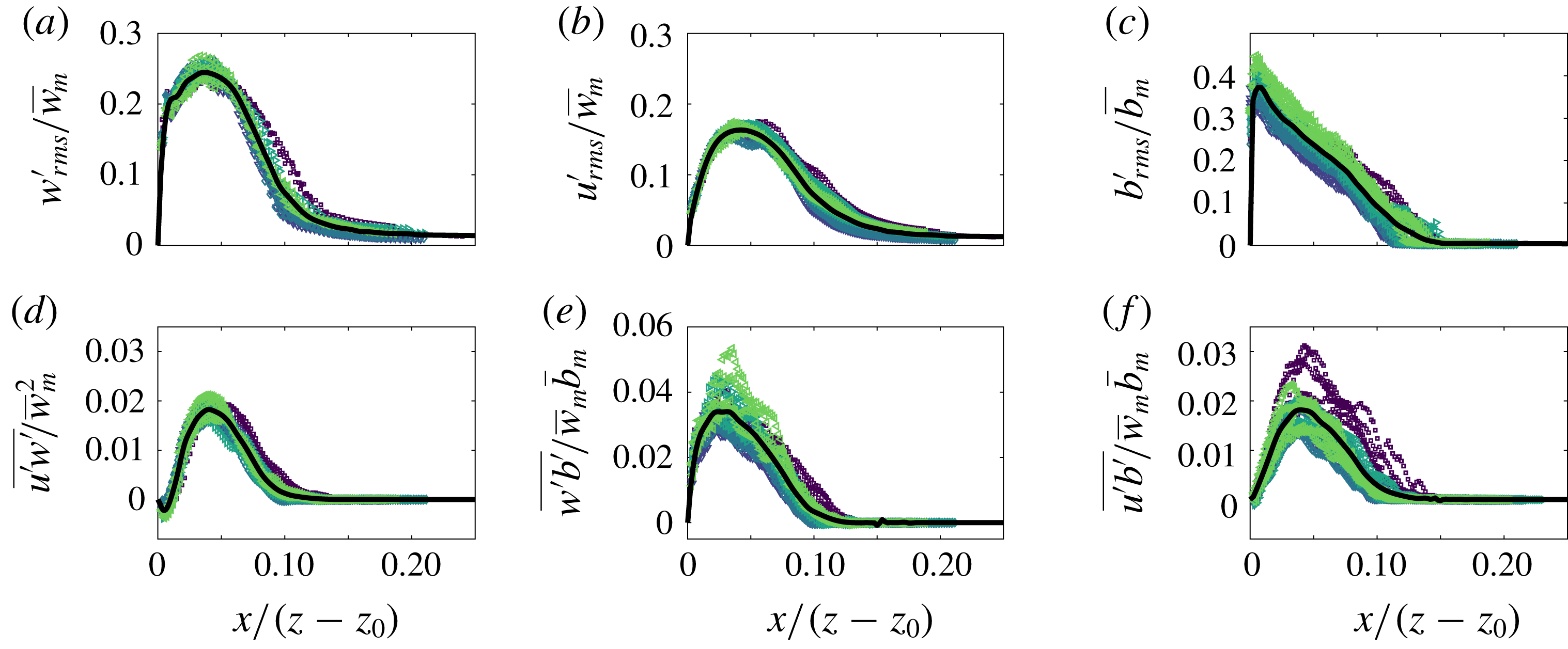
Time-averaged scaled wall plume turbulent fluctuations of (a) vertical velocity, (b) horizontal velocity, (c) buoyancy, (d) Reynolds stress, (e) vertical and (f) horizontal turbulent buoyancy flux. The black curves are the averages of the data.
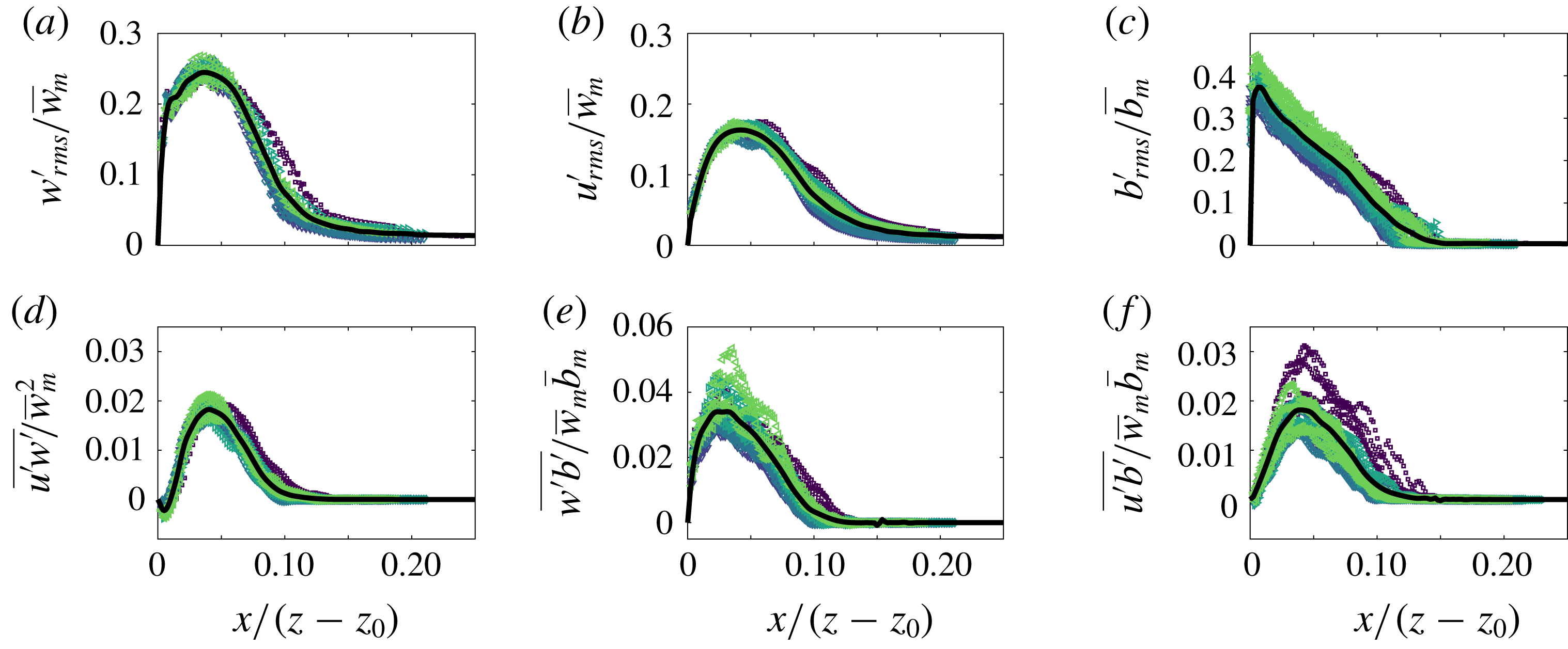
Measurements of velocity and buoyancy fluctuations, Reynolds stress and turbulent transport for the free and wall plume experiments are shown in figures 13 and 14, respectively, where the subscript
 $rms$
denotes the root mean square of the data. Our results for the free plume turbulent transport of buoyancy closely follow those of Ramaprian & Chandrasekhara (Reference Ramaprian and Chandrasekhara1989), and the turbulent buoyancy fluctuations are consistent with those of Sangras et al. (Reference Sangras, Dai and Faeth1998). For both plumes we note that the turbulent buoyancy fluxes are at most about 5 % of the mean vertical buoyancy flux. The turbulent fluctuations for the wall plume agree well with those of Sangras et al. (Reference Sangras, Dai and Faeth1999) and Sangras et al. (Reference Sangras, Dai and Faeth2000). To our knowledge, turbulent transport quantities for a wall plume in a self-similar region have not been calculated in previous studies, except within a developing region by Lai & Faeth (Reference Lai and Faeth1987). It is clear that their flow is not self-similar where their measurements were taken, and both the present study and Sangras et al. (Reference Sangras, Dai and Faeth2000) find significantly larger velocity turbulent fluctuations compared to Lai & Faeth (Reference Lai and Faeth1987) and, therefore, further comparison between our results is not insightful.
Larger maximum values for the normalised Reynolds stress of
 $0.30$
are found in the free plume compared with
 $0.22$
in the wall plume. The maximum values for the normalised turbulent horizontal and vertical fluxes are also significantly higher in the free plume being, in both cases, approximately double those of the wall plume. The kink observed in the vertical buoyancy flux, figure 14(e), at about
 $x/(z-z_{0})=0.08$
appears to be real, as opposed to resulting from scattered data, since it is reflected in the turbulent buoyancy fluctuations and also observed by Sangras et al. (Reference Sangras, Dai and Faeth1999).
5.6 Discussion
Our results may be set in context with the original observation of Ellison & Turner (Reference Ellison and Turner1959) that the reduced entrainment in the wall plume is due to the suppression of the meandering of the plume. We find that the meandering of the free plume creates coherent structures at the size of the total plume width that frequently overturn and engulf ambient fluid. This in turn stretches the interface leading to an increase in the total length of the TNTI and increased rates of entrainment (Ottino Reference Ottino1989). This suggests that the entrainment process may be viewed as a multi-scale continuous process, where ultimately, at the smallest scales, fluid is nibbled across the TNTI and then irreversibly mixed, consistent with the view of turbulent entrainment in axisymmetric jets (Mistry et al.
Reference Mistry, Philip, Dawson and Marusic2016), turbulent boundary layers (de Silva et al.
Reference de Silva, Philip, Chauhan, Meneveau and Marusic2013; Philip et al.
Reference Philip, Meneveau, de Silva and Marusic2014) and axisymmetric plumes (Burridge et al.
Reference Burridge, Parker, Kruger, Partridge and Linden2017). The observation that the total TNTI length of the free plume is 2.4 times that of the wall plume is then reflected well in the observation that the free plume entrains at a rate of approximately 2.4 times that of the wall plume. We find that the relative vertical transport of the engulfed fluid,
 $\overline{Q_{eng}}/\overline{Q}$
, of the free plume is approximately
 $18\,\%$
greater than the wall plume (see figure 12). However, the relative vertical transport of ambient fluid outside the TNTI envelope of the wall plume,
 $\overline{Q_{out}}/\overline{Q}$
, is approximately double that of the free plume. Further,
 $\overline{Q_{out}}$
and
 $\overline{Q_{eng}}$
are similar in the free plume whereas
 $\overline{Q_{out}}$
is almost double
 $\overline{Q_{eng}}$
in the wall plume, in addition to being much larger than both fluxes of the free plume. Thus the wall plume is relatively inefficient at engulfing the outer ambient fluid, although it transports relatively more unmixed fluid, that is
 $\overline{Q_{out}}$
and
 $\overline{Q_{eng}}$
combined, whereas the free plume is able to maintain a balance between the vertical transport of ambient and engulfed fluid.
6 Results in a plume coordinate system
6.1 Plume coordinate system definition
Following the analysis of Burridge et al. (Reference Burridge, Parker, Kruger, Partridge and Linden2017) of an axisymmetric plume, we examine the two flows in a coordinate system which follows the plumes as they fluctuate in width. For the free plume the coordinate system,
 $x_{p}(z,t)$
, is defined by the position of the outermost left,
 $x_{p}(z,t)=-X_{p}(z,t)=E_{L}(z,t)$
, and outermost right,
 $x_{p}(z,t)=X_{p}(z,t)=E_{R}(z,t)$
, points on the TNTI at a given height. The coordinate system for the wall plume is similarly defined, however
 $x_{p}(z,t)=0$
remains fixed at the wall, with
 $x_{p}(z,t)=X_{p}(z,t)$
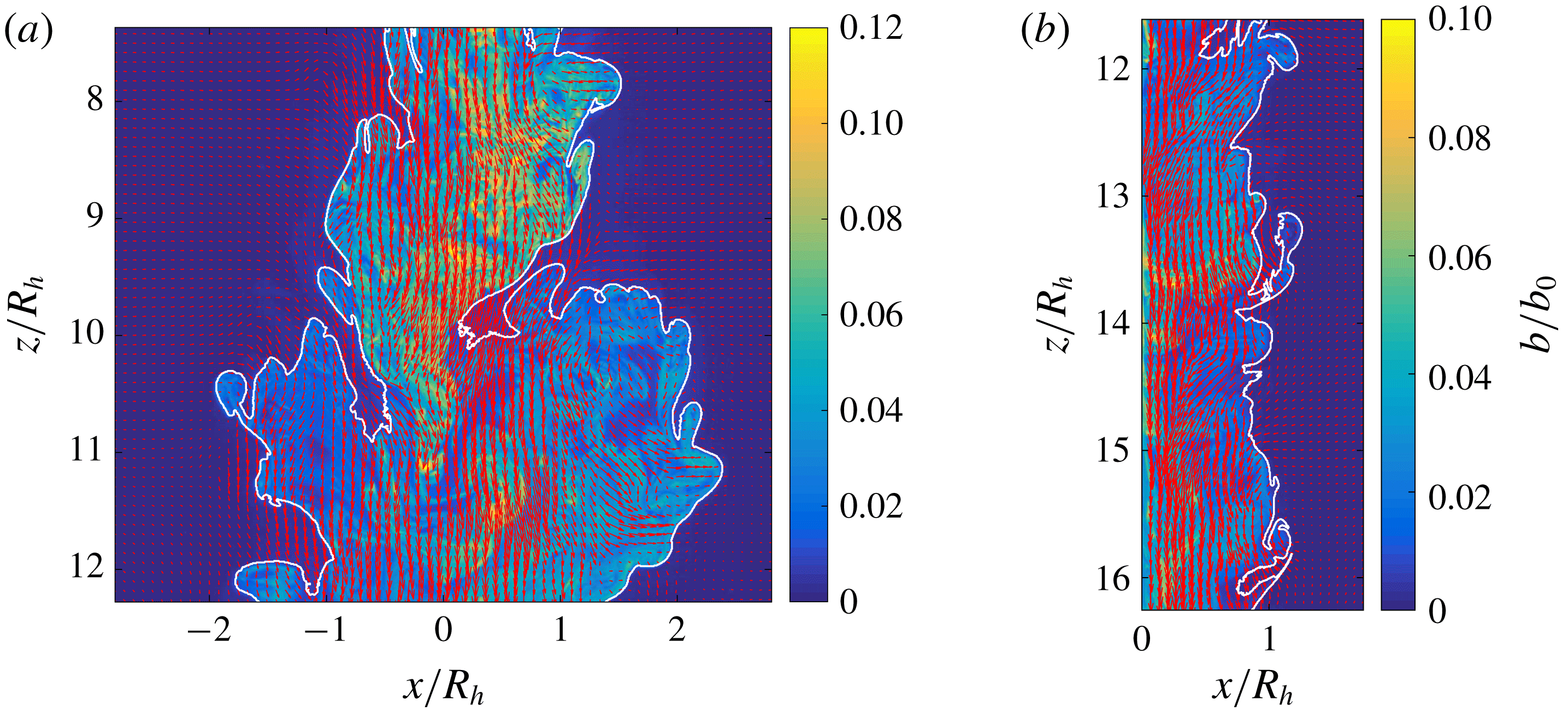
defined at the outermost TNTI position for a given height. Evidently from figure 15 multiple points along a TNTI can exist for a given height, so the outermost points along the TNTI are taken. Further, prior to the coordinate transformation, the data are conditioned on whether plume fluid is present within the outer plume envelope using the step function
 $H_{eng}$
, therefore ensuring that all statistics within the region
 $|x_{p}|<X_{p}$
are those within plume fluid. The time-averaged vertical velocity data in plume coordinates is then defined by
 $$\begin{eqnarray}\overline{w_{p}}=\overline{w(x_{p},z)}=\frac{1}{T_{c}}\int _{0}^{T}w(x_{p},z,t)[1-H_{eng}(x_{p},z,t)]\,\text{d}t,\end{eqnarray}$$
for the total recording time
 $T$
, where
 $T_{c}(x_{p},z)$
is the total amount of time at a given plume coordinate location when engulfed fluid is not present. This is necessary in order to omit engulfed regions within the plume from the conditional mean. The horizontal velocity
 $\overline{u_{p}}$
and buoyancy
 $\overline{b_{p}}$
are equivalently defined. The turbulent fluctuations and fluxes of the quantities in the plume coordinates are defined with respect to the time-averaged quantities in plume coordinates, e.g. for the turbulent vertical velocity fluctuations,
 $$\begin{eqnarray}w_{p,rms}^{\prime }=\left(\frac{1}{T_{c}}\int _{0}^{T}(w(x_{p},z,t)[1-H_{eng}(x_{p},z,t)]-\overline{w_{p}})^{2}\,\text{d}t\right)^{1/2},\end{eqnarray}$$
and equivalently for the horizontal velocity
 $u_{p,rms}^{\prime }$
and buoyancy fluctuations
 $b_{p,rms}^{\prime }$
.
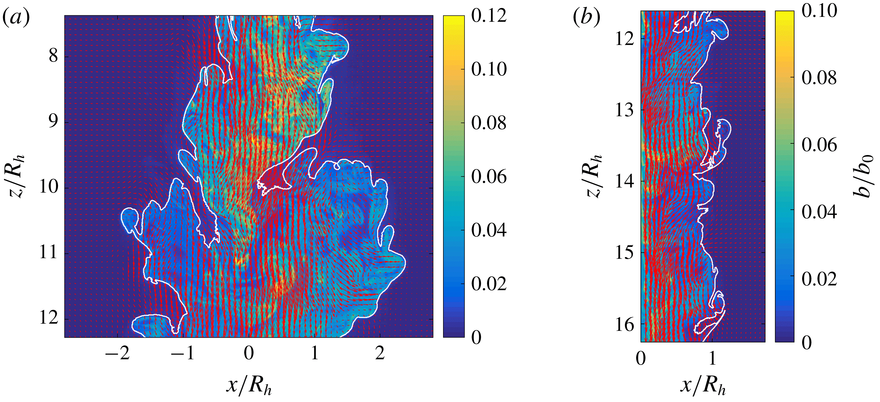
Instantaneous buoyancy field overlayed with velocity field (red arrows) from a (a) free and (b) wall plume experiment. The outer TNTI is highlighted in white.
6.2 Velocity and buoyancy in plume coordinates
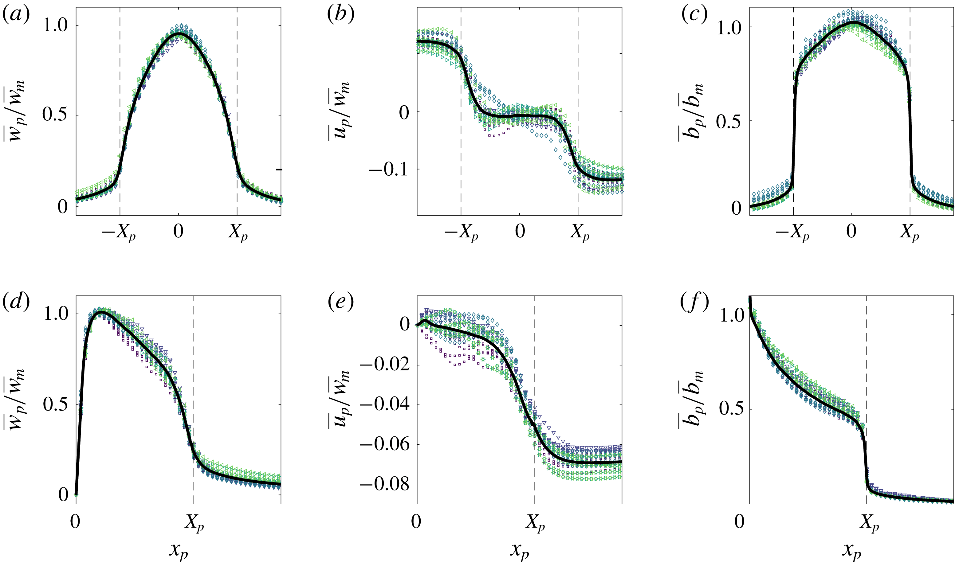
Time-averaged scaled vertical and horizontal velocity and buoyancy profiles of the (a–c) free and (d–f) wall plume in plume coordinates. For each experiment, five different heights spanning the studied region are plotted. The black dashed lines at
 $x_{p}=\{-X_{p},X_{p}\}$
highlight the position of the outer TNTI. The black curves are the averages of the data.
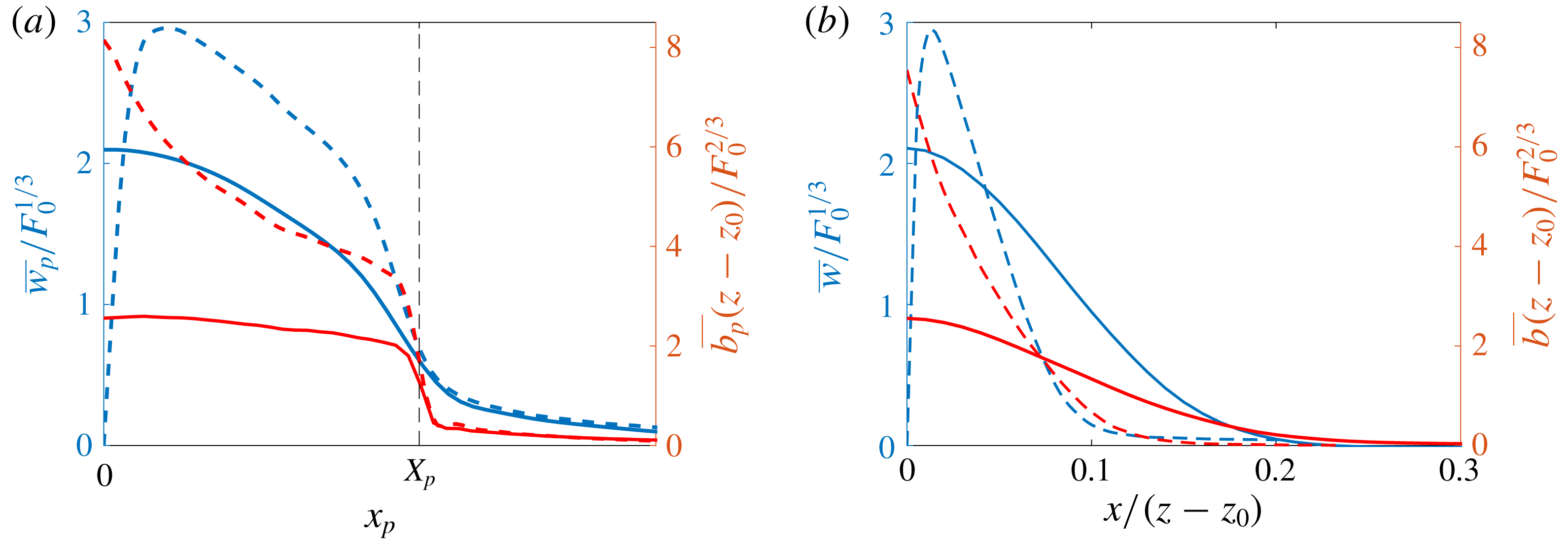
(a) Average profiles of the time-averaged free (solid) and wall plume (dashed) vertical velocities (blue, left) and buoyancy (red, right) in (a) plume coordinates and (b) Eulerian coordinates. Only half the region of the free plume is shown in both cases to aid comparison with the wall plume. Vertical velocities have been scaled using the buoyancy flux and buoyancy has been scaled using the buoyancy flux and distance from the virtual origin.
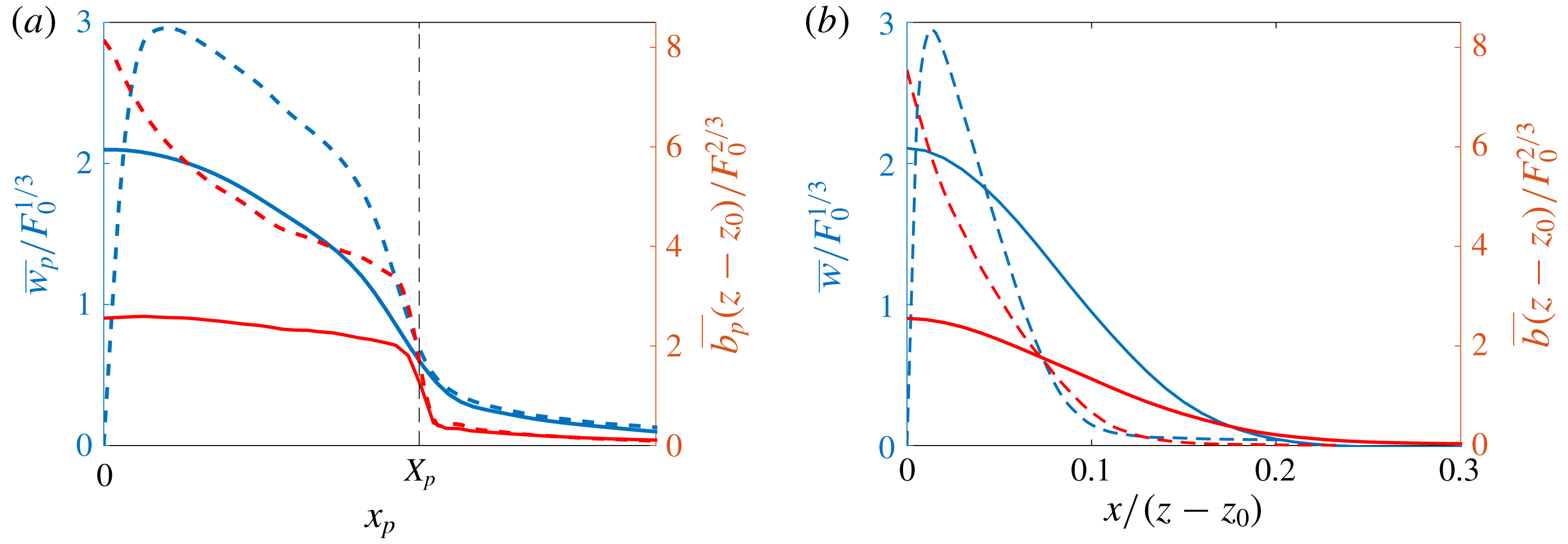
The conditionally averaged velocity and buoyancy data in plume coordinates across all experiments are shown in figure 16. Data were taken from five heights spanning the examined region for each experiment.
The average data for both sets of experiments collapse onto a single curve showing that the velocities and buoyancy are self-similar when viewed in plume coordinates. The vertical velocities and buoyancy have been scaled by the maximum, time-averaged, vertical velocity and buoyancy measured in Eulerian coordinates, respectively. The maximum time-averaged buoyancy in the plume coordinate system is greater than that in the Eulerian coordinate system for both the free and wall plume. This is to be expected, since the contribution of the ambient fluid in the calculation of the mean buoyancy is omitted in the plume coordinate system. However, it is surprising to note that the maximum vertical velocity of the free plume in the plume coordinate system is lower than that in the Eulerian coordinate system. This may be due to the meandering of the plume and is not observed in the wall plume where, as one would expect from considering the additional buoyancy, the maximum velocity is greater in the plume coordinate system.
The average vertical velocities at the plume edge (dashed vertical lines at
 $\{-X_{p},X_{p}\}$
) for the free plume are significant, on average
 $23\,\%$
of the centreline velocities. This is almost identical to the behaviour of an axisymmetric plume observed by Burridge et al. (Reference Burridge, Parker, Kruger, Partridge and Linden2017) where the vertical velocities at the outer TNTI of the plume were also found to be approximately
 $20\,\%$
of the centreline velocities. This behaviour is similarly observed in the wall plume where the vertical velocities at the outer TNTI are on average
 $25\,\%$
of the maximum vertical velocity.
The buoyancy profile in plume coordinates of the free plume in figure 16(c) shows that there is a jump in buoyancy at the interface to about
 $75\,\%$
of the centreline buoyancy within the plume. The jump in buoyancy is surprisingly large and significantly greater than the jump in passive scalar at the interface observed in an axisymmetric jet by Westerweel et al. (Reference Westerweel, Hofmann, Fukushima and Hunt2002). The jump in buoyancy at the interface for the wall plume figure 16(f) is significantly lower than the free plume at about
 $40\,\%$
of the maximum buoyancy. These jumps in buoyancy are almost identical to the jump observed from the conditional statistics in a coordinate system normal to the TNTI, shown in figure 4. The free plume buoyancy profile broadly exhibits a constant gradient, of opposite sign, either side of the centreline. This is in contrast to the wall plume, where the gradient is rapidly increasing in magnitude from the interface towards the wall.
To highlight differences between the two flows, figure 17(a) shows the average of all the data of the time-averaged vertical velocities and buoyancy in plume coordinates, and for comparison in Eulerian coordinates in figure 17(b), of the free and wall plume, where the vertical velocities have been scaled using the buoyancy flux and the buoyancy has been scaled using the buoyancy flux and virtual distance from the source. Only the region
 $x_{p}\geqslant 0$
is shown for the free plume. Figure 17(a) shows that, for a given buoyancy flux, the profiles of vertical velocity of the wall plume and free plume outside the plume are almost indistinguishable, in particular the vertical velocities at the outer TNTI,
 $x_{p}=X_{p}$
, are identical. Moving towards the wall, the vertical velocity of the wall plume increases away from the TNTI more rapidly than the free plume. This is expected given that the buoyancy in the wall plume is at least
 $1.6$
times greater than the free plume within the region
 $x_{p}/X_{p}<0.95$
. In the adjustment region,
 $0.95<x_{p}/X_{p}<1$
, the buoyancy rapidly increases for both the free and wall plume. However, away from this adjustment region within the plume,
 $x_{p}/X_{p}<0.95$
, the buoyancy of the free plume changes by at most
 $9\,\%$
of the mean buoyancy, whereas the wall plume changes by
 $52\,\%$
of the mean buoyancy within that region. This shows that in the free plume, plume fluid is more uniformly mixed than the wall plume. This implies that there is a more equal distribution of buoyancy force across the plume, which results in a more top-hat vertical velocity in plume coordinates, which can be seen in figure 17.
6.3 Turbulent fluctuations and fluxes in plume coordinates
Time-averaged scaled free plume turbulent fluctuations in plume coordinates of (a) vertical velocity, (b) horizontal velocity, (c) buoyancy, (d) Reynolds stress, (e) vertical and (f) horizontal turbulent buoyancy flux. The black curves are the averages of the data. A zero line is shown by the horizontal dashed line.
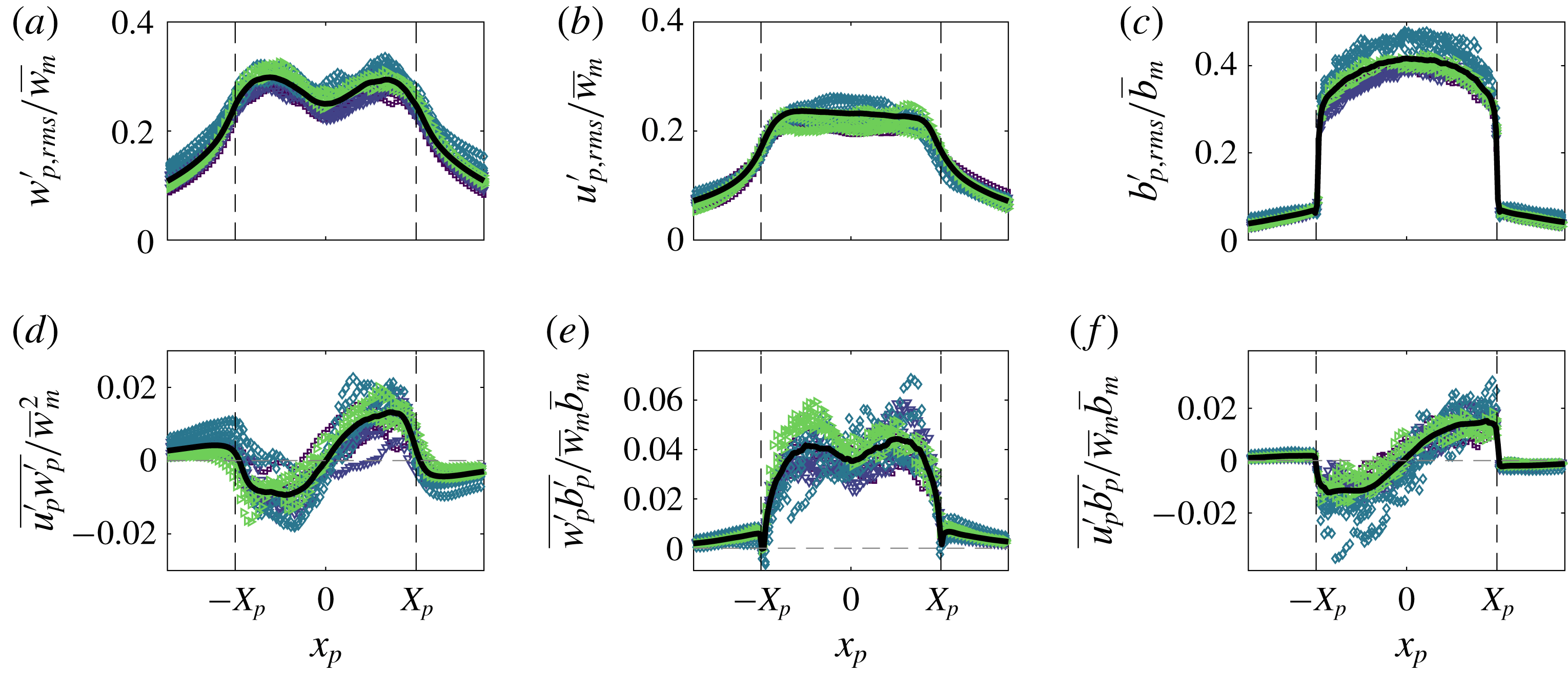
Time-averaged scaled wall plume turbulent fluctuations in plume coordinates of (a) vertical velocity, (b) horizontal velocity, (c) buoyancy, (d) Reynolds stress, (e) vertical and (f) horizontal turbulent buoyancy flux. The black curves are the averages of the data.
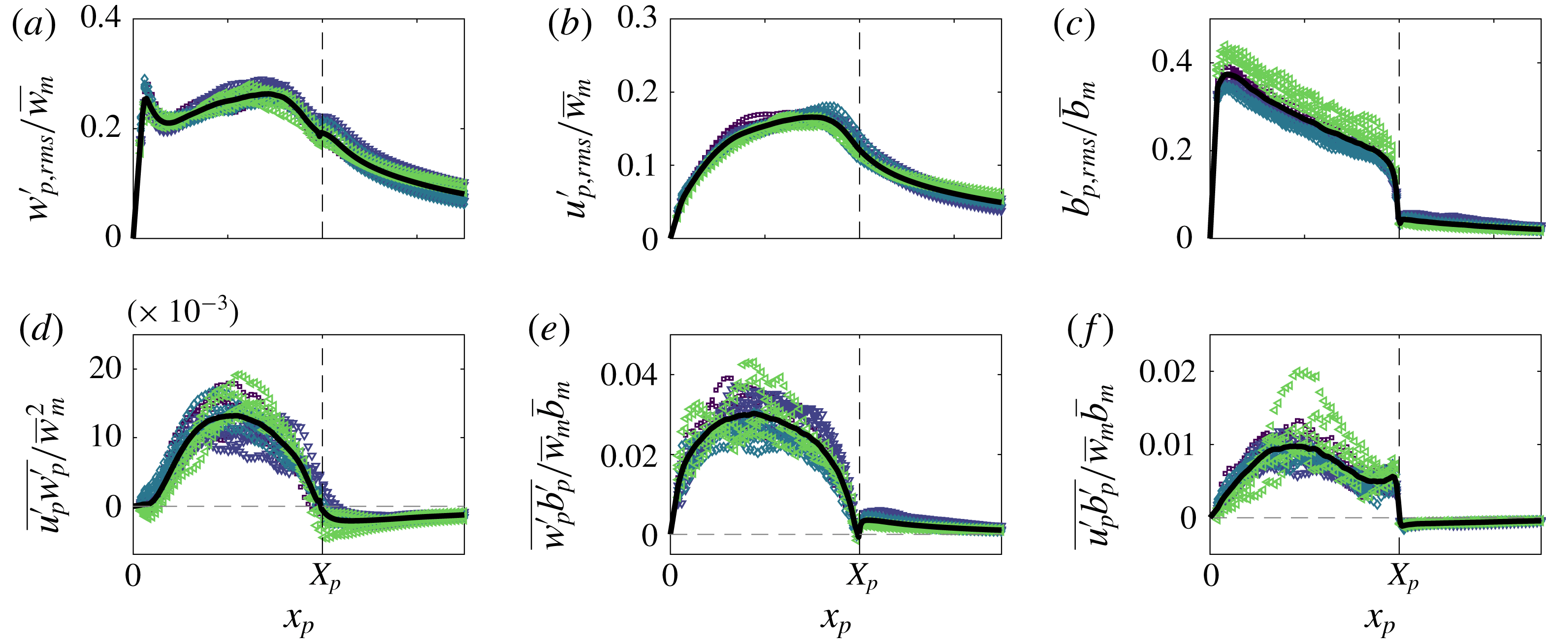
The vertical velocity fluctuations in plume coordinates are shown in figures 18(a) and 19(a) for the free and wall plume, respectively. The profile of the free plume broadly mirrors that observed in Eulerian space, with bi-modal peaks at
 $30\,\%$
of the maximum Eulerian vertical velocity. This is larger than the bi-modal peaks observed in Eulerian space, a result similarly observed in axisymmetric plumes (Burridge et al.
Reference Burridge, Parker, Kruger, Partridge and Linden2017), where it was suggested that the meandering of the plume masks the scale of the turbulent velocity fluctuations. The profile of the vertical velocity fluctuations in the wall plume is quite different from Eulerian space. Three distinct peaks are observed: one very close to the wall, a second peak within the middle of the plume region and a third peak almost exactly at the outer TNTI of the plume. The maximum peak is on average
 $25\,\%$
of the maximum Eulerian vertical velocity. This peak value is almost identical to that observed in Eulerian space. The reduced meandering of the wall plume may explain the reduced effect of the increase in magnitude of turbulent velocity fluctuations seen in the free and axisymmetric plume.
The buoyancy fluctuations of the free and the wall plume in figures 18(c) and 19(c), respectively, are very different to the Eulerian statistics. This is expected, since there must be ambient fluid, i.e.
 $b=0$
(except for any additional noise associated with the experiment), beyond the outer TNTI and therefore a jump is observed at
 $x_{p}=\pm X_{p}$
in both flows. The maximum buoyancy fluctuations in both the free and wall plume are less than those in the Eulerian statistics. This results from the condition that the ambient fluid is omitted in the calculation of the statistic. A larger discrepancy between the plume and Eulerian coordinate system is observed in the free plume, owing to the increased meandering and engulfment of the free plume.
The Reynolds stress profiles of the free and the wall plume in plume coordinates are shown in figures 18(d) and 19 (d), respectively. An interesting feature, which is also observed in axisymmetric plumes (Burridge et al.
Reference Burridge, Parker, Kruger, Partridge and Linden2017), is the change of sign across the region of the plume edge. For comparison consider only the region
 $x_{p}\geqslant 0$
of the free plume, but note that results are equivalent although of opposite sign for
 $x_{p}\leqslant 0$
. In this case, as with the wall plume in the region away from the wall,
 $\overline{u_{p}^{\prime }w_{p}^{\prime }}$
is positive within the plume, however it rapidly becomes negative within the ambient fluid. This is in contrast to the Eulerian statistic, where
 $\overline{u^{\prime }w^{\prime }}$
is positive and gradually tends to zero in the positive
 $x$
direction, because the Reynolds stress is larger in magnitude within the plume region and, as with the velocity fluctuations, the meandering of the plume masks the ambient flow statistics. The negative Reynolds stress outside the plume may be explained from considering the entrainment process. The negative correlation
 $\overline{u_{p}^{\prime }w_{p}^{\prime }}<0$
results from either transport of streamwise momentum inwards or transport of negative streamwise momentum outwards. The former is consistent with the observation that
 $w_{p,rms}^{\prime }>0$
(figures 18
a and 19
a) and is associated with entrainment since it is necessary for transport of fluid from the non-turbulent ambient into the turbulent plume region, as described by Odier, Chen & Ecke (Reference Odier, Chen and Ecke2012) for a gravity current. The latter would imply detrainment of slower moving plume fluid which is not observed. The peak Reynolds stresses in plume coordinates, in both cases, are lower in magnitude than the Eulerian Reynolds stresses. This is also observed in axisymmetric plumes and it is not yet clear why this should occur.
The turbulent vertical buoyancy flux in plume coordinates of the free plume (figure 18
e) shows a bi-modal peak with maximum values on average
 $30\,\%$
larger than those observed in Eulerian coordinates. The omission of ambient data has a similar effect on reducing
 $\overline{w_{p}^{\prime }b_{p}^{\prime }}$
. The turbulent buoyancy flux in plume coordinates of the wall plume, figure 19(e), looks quite different from the Eulerian statistic. The profile is more similar to a top-hat profile, and the kink seen in Eulerian coordinates is not observed. This, therefore, suggests the kink is a consequence of the combined ambient and plume statistics in the Eulerian coordinate system, especially since it is located close to the mean position of the plume edge.
6.4 Summary of results in the plume coordinate
As shown in figure 17 the vertical velocity and buoyancy profiles in the ambient fluid immediately outside the plume are the same for both the free and the wall plume. This similarity is not apparent from the Eulerian data and neither are the large gradients in vertical velocity and buoyancy at the plume edge. The plume-coordinate data also show that the fluctuations in vertical velocity at the plume edge are larger than those revealed by the Eulerian data. The fluctuations in buoyancy are also significantly different when observed in plume coordinates, since the Eulerian statistics smear the data between the plume and the ambient fluid.
The plume-coordinate data also reveal aspects concerning the entrainment process that are not evident from the Eulerian data. For example, in plume coordinates the Reynolds stress changes sign outside the plume (a change not apparent in Eulerian coordinates), which as described above is a result of ambient fluid being drawn towards the plume. Further comparison of figures 18(d) and 19(d) show that the reduced entrainment in the wall plume compared to the free plume is consistent with the smaller magnitude of the Reynolds stress outside the plume in the latter case.
7 Conclusions
Simultaneous velocity and buoyancy field measurements of a free and wall plume provided direct measurements of the top-hat entrainment coefficients. We found that the entrainment coefficient of the free plume
 $\unicode[STIX]{x1D6FC}_{f}=0.14$
is slightly less than double that of the wall plume
 $\unicode[STIX]{x1D6FC}_{w}=0.08$
. However, it was shown that, for a given buoyancy flux, this corresponds to the free plume physically entraining more than double per unit height than the wall plume, as expressed in terms of the rate of increase in plume volume flux with height
 $\text{d}Q_{f}/\text{d}z=2.4\,\text{d}Q_{w}/\text{d}z$
.
To examine this difference the entrainment coefficient of the wall plume was decomposed and the relative contributions from turbulence production, buoyant and viscous terms were compared to the free plume decomposition first performed by Paillat & Kaminski (Reference Paillat and Kaminski2014a
). A significant reduction in
 $\unicode[STIX]{x1D6FC}_{production}$
, approximately equal to the negative contribution from the viscous terms
 $\unicode[STIX]{x1D6FC}_{viscous}$
, is found in the wall plume. This suggests both the reduction in turbulent production and viscous dissipation due to the wall boundary layer, which indirectly affects entrainment by providing an energy sink (Holzner et al.
Reference Holzner, van Reeuwijk and Jonker2016), are significant in the reduction of entrainment.
The statistics of the TNTI were calculated. We provided evidence of the free plume meandering and, in particular, we showed that there is a significant probability, approximately
 $15\,\%$
, of ambient fluid outside the plume TNTI existing at the centreline, suggesting coherent lateral/sideways meandering of the plume centreline. This is in contrast to an axisymmetric plume where no coherence between the left and right TNTI of the plume were observed (Burridge et al.
Reference Burridge, Parker, Kruger, Partridge and Linden2017). Through this meandering it was shown that the TNTI is stretched and on average the total length of TNTI of the free plume is longer than the wall plume by a factor of at least 2.2, measured at intermediate length scales.
The turbulent velocity and buoyancy fluctuations were measured and the resulting turbulent fluxes and Reynolds stresses were calculated. Larger peak values were observed across all the fluctuations and turbulent fluxes in the free plume, resulting from larger turbulence production in the free plume. When the data are analysed in plume coordinates we find that the mean vertical velocity and buoyancy profiles in the ambient fluid are essentially the same, but the magnitude of the Reynolds stress is smaller in the wall plume consistent with the reduced entrainment rate compared with the free plume.
While the presence of the wall is the only fundamental difference between the free and wall plume, the effect of the wall could be viewed as two separate processes, namely the no-slip condition and the impermeability condition. We show that the wall shear stress is non-negligible and this results in a reduction of momentum of the wall plume, which could otherwise be used in the turbulent production contributing to entrainment. Alternatively, the impermeability condition prevents the wall plume meandering which both reduces the large-scale engulfment process and the stretching of the TNTI leading to a shorter total TNTI. As mentioned above this also manifests itself in smaller Reynolds stresses in the wall plume at the edge of the plume. It is difficult to separate these two processes and provide an answer to which is the dominant effect in the reduction of entrainment in the wall plume, however the entrainment coefficient decomposition suggests that they are approximately equal in importance. It would be interesting to resolve this issue numerically by comparing a simulation of a wall plume with a no-slip and a free-slip condition, as performed for a gravity current in Holzner et al. (Reference Holzner, van Reeuwijk and Jonker2016).
Acknowledgements
We are grateful to the skilled technical staff of the G. K. Batchelor Laboratory for the manufacture of the apparatus and the illumination system. We also wish to acknowledge the contribution of Professor S. Dalziel to the data capture and processing. The work has received financial support from the UK Engineering and Physical Sciences Research Council through an iCASE award with Arup, the First Grant EP/R008957/1 ‘Confinement, boundaries and buoyancy in the mixing by fluid flows’ and also through the Programme Grant EP/K034529/1 ‘Mathematical Underpinnings of Stratified Turbulence’ (MUST), and from the European Research Council through the Horizon 2020 research and innovation programme agreement no. 742480 ‘Stratified turbulence and mixing processes’ (STAMP). The data associated with this paper can be found in the repository https://doi.org/10.17863/CAM.44080.
Appendix A. LIF attenuation analysis
Here we assess the error associated with the LIF density measurements due to the attenuation as a result of the Rhodamine
 $6$
G dye and added salts, and justify performing a two-point calibration.
A two-point calibration relies on the assumption that the local illumination intensity between the calibration image of mixed dye,
 $I_{m}(x,z)$
, and the background,
 $I_{b}(x,z)$
, are approximately equal. Further, that the local illumination intensity between the calibration images and the experiment,
 $I(x,z,t)$
, are also approximately equal. Typically, however, the local illumination intensity in an experiment is not known since it varies spatially and temporally as a function of the absorption of the laser light that occurs along its path (Crimaldi Reference Crimaldi2008) or, as it is typically referred to, attenuation. The Bouguer–Lambert–Beer law may be used to relate the local illumination intensity of a reference medium,
 $I_{0}(x,z)$
, to the local illumination intensity,
 $I(x,z,t)$
, in an absorbing medium, where the light is assumed to travel parallel to the
 $z$
direction, as follows
 $$\begin{eqnarray}I(x,z,t)=I_{0}(x,z)\exp \left(-\int _{0}^{z}\mathop{\sum }_{i=1}^{N}\unicode[STIX]{x1D716}_{i}c_{i}(x,z^{\prime },t)\,\text{d}z^{\prime }\right),\end{eqnarray}$$
where
 $\unicode[STIX]{x1D716}_{i}$
are the extinction coefficients of the absorbing media with concentrations
 $c_{i}$
.
Schematic of the free plume experiment highlighting the features used in the laser beam attenuation analysis.
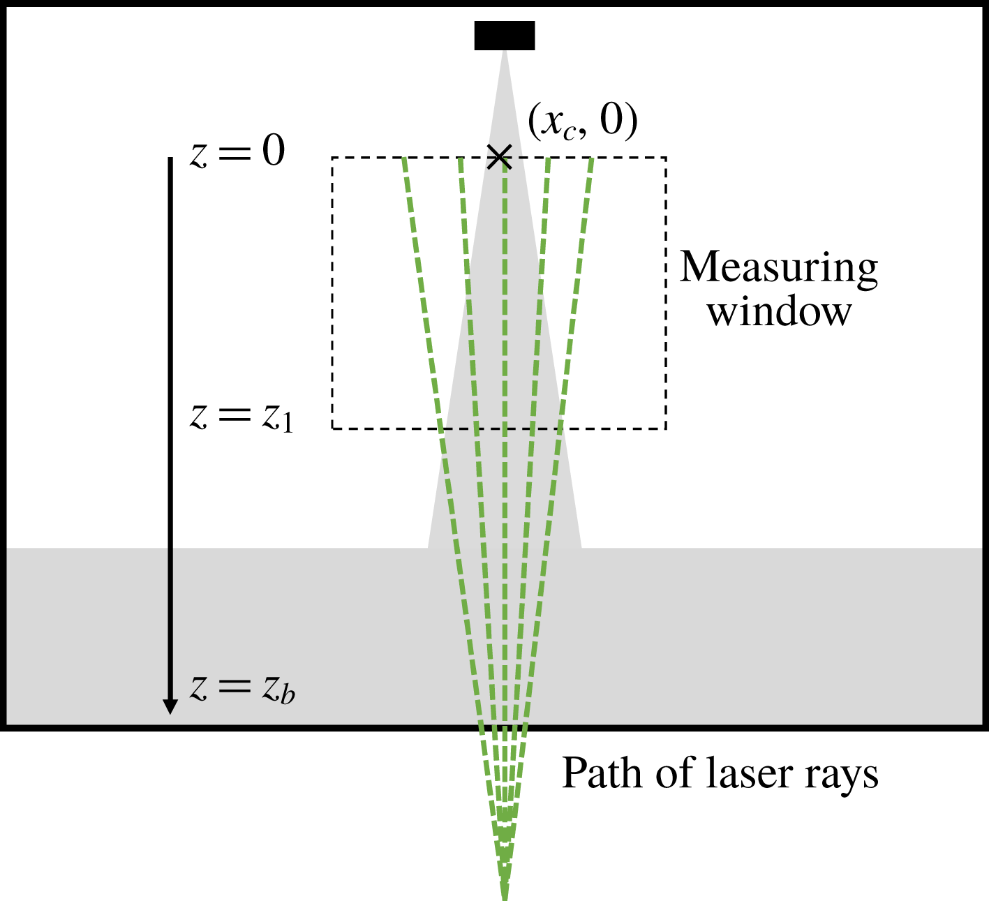
First we consider the free plume experiments. In order to describe the analysis we consider experiment
 $1$
, however, we give the analogous final results at the end of this section for all the experiments. The measurement window is 16 cm in height and the bottom of the measurement window
 $z_{1}$
, with
 $z=0~\text{cm}$
at the top of the measurement window (see figure 20), is at a distance 32.5 cm from the base of the tank. The path of the light rays along the mean centreline of the plume were approximately parallel to the
 $z$
direction. Given that the maximum dye attenuation due to the plume is likely to occur along the mean centreline of the plume we consider the local illumination intensity at the maximum height from the base of the tank, which is at
 $z_{b}=48.5~\text{cm}$
, within the measurement window at the centreline
 $x_{c}$
of the plume, and we make the assumption that the path of the laser travels along the path
 $x=x_{c}$
.
We define the local illumination intensity at the position
 $(x_{c},0)$
(the position of the cross in figure 20) in the tank containing fresh water by
 $I_{0}$
. We define the local illumination intensity in the tank containing a sodium chloride (NaCl) solution concentration,
 $c_{s}$
, at the same point by
 $I_{b}$
. These may be related to each other using (A 1) by
 $$\begin{eqnarray}I_{b}=I_{0}\exp (-\unicode[STIX]{x1D716}_{s}c_{s}z_{b}),\end{eqnarray}$$
where
 $\unicode[STIX]{x1D716}_{s}$
is the extinction coefficient for NaCl.
The background calibration image used in the two-point calibration contained NaCl solution at the concentration used in the ambient fluid of the experiments. The intensity
 $I_{b}$
may therefore be considered as the background calibration image. The intensity of the mixed calibration image,
 $I_{m}$
, of a known concentration,
 $c_{d}$
, of Rhodamine
 $6G$
with the same NaCl solution as
 $I_{b}$
may be related to the background image by
 $$\begin{eqnarray}I_{m}=I_{b}\exp (-\unicode[STIX]{x1D716}_{d}c_{d}z_{b}),\end{eqnarray}$$
where
 $\unicode[STIX]{x1D716}_{d}$
is the extinction coefficient for Rhodamine
 $6G$
.
For an experiment with initial ambient NaCl concentration
 $c_{s,0}$
and source sodium nitrate (
 $\text{NaNO}_{3}$
) and Rhodamine
 $6G$
concentration
 $c_{n,0}$
and
 $c_{d,0}$
, respectively, the local illumination intensity during the experiment is given by
 $$\begin{eqnarray}I(t)=I_{0}\exp \left(-\int _{0}^{z_{b}}\unicode[STIX]{x1D6FE}\unicode[STIX]{x1D716}_{d}c_{d,0}+\unicode[STIX]{x1D6FE}\unicode[STIX]{x1D716}_{n}c_{n,0}+(1-\unicode[STIX]{x1D6FE})\unicode[STIX]{x1D716}_{s}c_{s,0}\,\text{d}z\right),\end{eqnarray}$$
where
 $\unicode[STIX]{x1D716}_{n}$
is the extinction coefficient for
 $\text{NaNO}_{3}$
and
 $\unicode[STIX]{x1D6FE}=\unicode[STIX]{x1D6FE}(z,t)$
is the plume fluid concentration relative to the source solution, i.e.
 $\unicode[STIX]{x1D6FE}=0$
in the unmixed ambient fluid and
 $\unicode[STIX]{x1D6FE}=1$
in the unmixed source solution. The relation (A 4) can be written in terms of
 $I_{b}$
as follows:
 $$\begin{eqnarray}\displaystyle I(t) & = & \displaystyle I_{b}\exp \left(-\int _{0}^{z_{b}}\unicode[STIX]{x1D6FE}\unicode[STIX]{x1D716}_{d}c_{d,0}+\unicode[STIX]{x1D6FE}\unicode[STIX]{x1D716}_{n}c_{n,0}-\unicode[STIX]{x1D6FE}\unicode[STIX]{x1D716}_{s}c_{s,0}\,\text{d}z\right),\end{eqnarray}$$
 $$\begin{eqnarray}\displaystyle & = & \displaystyle I_{b}\exp \left(-(\unicode[STIX]{x1D716}_{d}c_{d,0}+\unicode[STIX]{x1D716}_{n}c_{n,0}-\unicode[STIX]{x1D716}_{s}c_{s,0})\int _{0}^{z_{b}}\unicode[STIX]{x1D6FE}\,\text{d}z\right),\end{eqnarray}$$
 $$\begin{eqnarray}\displaystyle & = & \displaystyle I_{b}\exp \left(-z_{b}(\unicode[STIX]{x1D716}_{d}c_{d,0}+\unicode[STIX]{x1D716}_{n}c_{n,0}-\unicode[STIX]{x1D716}_{s}c_{s,0})\frac{1}{z_{b}}\int _{0}^{z_{b}}\unicode[STIX]{x1D6FE}\,\text{d}z\right).\end{eqnarray}$$
The value
 $(1/z_{1})\int _{0}^{z_{1}}\unicode[STIX]{x1D6FE}\,\text{d}z^{\prime }$
for each image may be estimated directly from the LIF measurements. The measurements from experiment
 $1$
give a time-averaged value of
 $$\begin{eqnarray}\frac{1}{T}\frac{1}{z_{1}}\int _{0}^{T}\int _{0}^{z_{1}}\unicode[STIX]{x1D6FE}\,\text{d}z\,\text{d}t=0.0396,\end{eqnarray}$$
with a standard deviation of
 $\unicode[STIX]{x1D70E}=0.0050$
and a maximum value of
 $0.0550$
. In order to provide a reasonable estimate for the worst-case attenuation for the region below the measurement window, considering the additional dilution that will result, we assume that
 $\unicode[STIX]{x1D6FE}(z)=\overline{\unicode[STIX]{x1D6FE}(z_{1})}=0.0232$
for
 $z>z_{1}$
, where
 $\overline{\unicode[STIX]{x1D6FE}}$
is the time average of
 $\unicode[STIX]{x1D6FE}$
.
By assuming the worst-case value for the measurement window,
 $\unicode[STIX]{x1D6FE}(z)=0.0565$
, we find that
 $$\begin{eqnarray}\frac{1}{z_{b}}\int _{0}^{z_{b}}\unicode[STIX]{x1D6FE}\,\text{d}z=0.0373.\end{eqnarray}$$
In order to determine the extinction coefficients for the Rhodamine
 $6$
G and the added salts, a calibration was performed with full details given in appendix B. We find values of
 $\unicode[STIX]{x1D716}_{d}=1.64\times 10^{-4}~\text{cm}^{-1}(\unicode[STIX]{x03BC}\text{g}/\text{l})^{-1}$
,
 $\unicode[STIX]{x1D716}_{s}=4.2\times 10^{-5}~\text{cm}^{-1}(\text{g}/\text{l})^{-1}$
and
 $\unicode[STIX]{x1D716}_{n}=8.8\times 10^{-6}~\text{cm}^{-1}(\text{g}/\text{l})^{-1}$
. The concentrations used in the free plume experiment
 $1$
were
 $c_{d,0}=200~\unicode[STIX]{x03BC}\text{g}~\text{l}^{-1}$
,
 $c_{s,0}=78~\text{g}~\text{l}^{-1}$
and
 $c_{n,0}=120~\text{g}~\text{l}^{-1}$
. Using the extinction coefficient for the Rhodamine
 $6$
G and concentration used in the mixed calibration image,
 $c_{d}=6.7~\unicode[STIX]{x03BC}\text{g}~\text{l}^{-1}$
, gives
 $$\begin{eqnarray}I_{m}=0.949I_{b}.\end{eqnarray}$$
This implies the local illumination intensity is at most
 $5.1\,\%$
smaller in the mixed calibration than the background calibration. For the experimental images, from the relation (A 7), we find that
 $$\begin{eqnarray}I=0.948I_{b},\end{eqnarray}$$
which shows that the local illumination intensity is at most
 $5.2\,\%$
less in any experiment than the background calibration. Importantly, this suggests that the maximum difference between the intensity of any two of the three images is less than
 $5.2\,\%$
. Table 5 shows the analogous results results for all the free plume experiments showing that across all the experiments the error due to the attenuation was at most
 $5.5\,\%$
.
Extinction coefficient calibration experiments for Rhodamine 6G (a) and the salts (b). The best fit lines (dashed) yield
 $\unicode[STIX]{x1D716}_{d}=1.64\times 10^{-4}~\text{cm}^{-1}(\unicode[STIX]{x03BC}\text{g}/\text{l})^{-1}$
,
 $\unicode[STIX]{x1D716}_{n}=1.406\times 10^{-2}~\text{cm}^{-1}(\unicode[STIX]{x0394}\unicode[STIX]{x1D70C}_{n})^{-1}$
and
 $\unicode[STIX]{x1D716}_{s}=6.094\times 10^{-2}~\text{cm}^{-1}(\unicode[STIX]{x0394}\unicode[STIX]{x1D70C}_{s})^{-1}$
, where
 $\unicode[STIX]{x0394}\unicode[STIX]{x1D70C}_{s/n}=\unicode[STIX]{x1D70C}_{s/n}-\unicode[STIX]{x1D70C}_{0}$
and
 $\unicode[STIX]{x1D70C}_{0}$
is the density of fresh water.
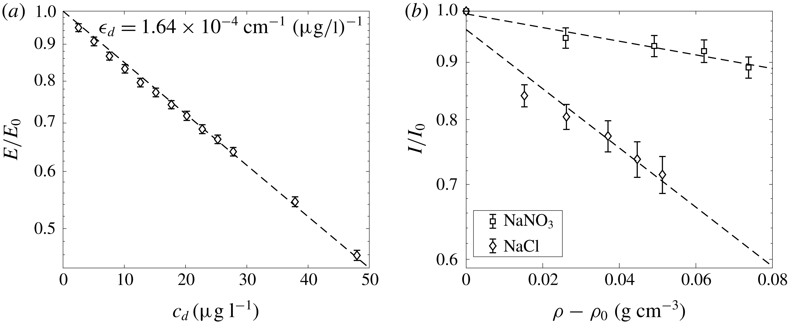
Relative attenuation of the mixed calibration image to the background image,
 $I_{m}/I_{b}$
, and the maximum attenuation of the experimental images relative to the background image,
 $\min (I/I_{b})$
, of the experiments.

An equivalent analysis may be performed for the wall plume where
 $z_{1}=15.7~\text{cm}$
and
 $z_{b}=35.2~\text{cm}$
. The analogous values to those calculated for the free plume are also given in table 5 which shows that across all the wall plume experiments the error due to the attenuation was at most
 $5.6\,\%$
.
Appendix B. Calibration of extinction coefficients
A series of calibration experiments were performed to determine the extinction coefficients
 $\unicode[STIX]{x1D716}_{d}$
,
 $\unicode[STIX]{x1D716}_{n}$
and
 $\unicode[STIX]{x1D716}_{s}$
. For the Rhodamine 6G coefficient,
 $\unicode[STIX]{x1D716}_{d}$
, the laser system was positioned so that the beam passed through a 1 m long tank before reaching a Gentec-eo energy meter (model QE25LP-H-MB). To perform the calibration, first a background state
 $E_{0}$
was recorded with the tank filled with fresh water and then the average energy of 1000 pulses was logged on the energy meter. Subsequent recordings were made after incrementally adding Rhodamine 6G dye to the calibration tank. The decay of the energy
 $E$
, due to attenuation, can be seen in figure 21. From these data, we find that
 $\unicode[STIX]{x1D716}_{d}=1.64\times 10^{-4}~\text{cm}^{-1}(\unicode[STIX]{x03BC}\text{g}/\text{l})^{-1}$
, as shown by the dashed line in figure 21.
The same calibration procedure was attempted for the salts, however, due to refractive index changes, the energy meter did not appear to be a robust method of capturing the attenuation. Therefore, a different calibration procedure was utilised for the salts. The same 1 m long tank was used but, instead of the laser, a DC powered LED light bank provided illumination. The light from the LED bank travelled through the length of the tank (1 m) before being recorded by a Dalsa Falcon2 4 MP CMOS camera fitted with a bandpass filter centred at the wavelength of the laser (532 nm), to ensure we are only measuring the extinction coefficient at the appropriate wavelength. Just as a dye attenuation system would be calibrated, a background image was captured with fresh water
 $I_{0}$
and subsequent images
 $I$
were captured for various salt concentrations. Figure 21 shows the calibration results using this methodology for the salts where we find
 $\unicode[STIX]{x1D716}_{n}=1.406\times 10^{-2}~\text{cm}^{-1}(\unicode[STIX]{x0394}\unicode[STIX]{x1D70C}_{n})^{-1}$
and
 $\unicode[STIX]{x1D716}_{s}=6.094\times 10^{-2}~\text{cm}^{-1}(\unicode[STIX]{x0394}\unicode[STIX]{x1D70C}_{s})^{-1}$
as the extinction coefficients for
 $\text{NaNO}_{3}$
and NaCl, respectively. Here,
 $\unicode[STIX]{x0394}\unicode[STIX]{x1D70C}_{s/n}$
signifies the change in density due to the corresponding salt, subscript
 $s$
for NaCl and
 $n$
for
 $\text{NaNO}_{3}$
, where
 $$\begin{eqnarray}\displaystyle & \displaystyle \unicode[STIX]{x0394}\unicode[STIX]{x1D70C}_{s} & \displaystyle =0.000685c_{s},\end{eqnarray}$$
 $$\begin{eqnarray}\displaystyle & \displaystyle \unicode[STIX]{x0394}\unicode[STIX]{x1D70C}_{n} & \displaystyle =0.000628c_{n},\end{eqnarray}$$
which results in the extinction coefficients
 $\unicode[STIX]{x1D716}_{s}=4.2\times 10^{-5}~\text{cm}^{-1}(\text{g}/\text{l})^{-1}$
and
 $\unicode[STIX]{x1D716}_{n}=8.8\times 10^{-6}~\text{cm}^{-1}(\text{g}/\text{l})^{-1}$
.