The data may not contain the answer. The combination of some data and an aching desire for an answer does not ensure that a reasonable answer can be extracted from a given body of data (Tukey Reference Tukey1986, 74).
Social scientists often face situations, known as “partial observability,” where two (or perhaps more) distinct processes lead to distinct binary outcomes that can only be observed jointly. Braumoeller (Reference Braumoeller2003) provides many examples of established literature theorizing such relationships. For example, survey respondents might self-report turning out to vote because (1) they actually voted or (2) they feel social pressure to do so. Similarly, two states will only sign a treaty if both states want the treaty. In these examples, researchers might be interested in modeling the decision to actually vote or the decision of a single state to want a treaty. Econometricians and methodologists argue that researchers can use a partial observability model to parse out the effects of a single explanatory variable on each unobserved outcome (Poirier Reference Poirier1980; Abowd and Farber Reference Abowd and Farber1982; Przeworski and Vreeland Reference Przeworski and Vreeland2002; Xiang Reference Xiang2010; Nieman Reference Nieman2015). This partial observability model is also referred to as the split population logit (Beger et al. Reference Beger, DeMeritt, Hwang and Moore2011) and the Boolean logit or probit (Braumoeller Reference Braumoeller2003).
Partial observability models inform the literatures on important processes and outcomes such as civil wars (Nieman Reference Nieman2015), international conflict and trade (Xiang Reference Xiang2010), International Monetary Fund (IMF) agreements (Knight and Santaella Reference Knight and Santaella1997; Przeworski and Vreeland Reference Przeworski and Vreeland2000; Przeworski and Vreeland Reference Przeworski and Vreeland2002; Vreeland Reference Vreeland2003; Stone Reference Stone2008), union membership (Abowd and Farber Reference Abowd and Farber1982), regulatory compliance (Feinstein Reference Feinstein1990; Stafford Reference Stafford2002; Chen et al. Reference Chen, Firth, Gao and Rui2006; Wang Reference Wang2013), network formation (Comola and Fafchamps Reference Comola and Fafchamps2014), credit ratings (Boyes, Hoffman and Low Reference Boyes, Hoffman and Low1989), agricultural innovation (Dimara and Skuras Reference Dimara and Skuras2003), health insurance ownership (Amir Reference Amir2001), and employment discrimination (Heywood and Mohanty Reference Heywood and Mohanty1990; Logan Reference Logan1996; Mohanty Reference Mohanty2002). Feinstein (Reference Feinstein1990) suggests the model’s usefulness for a wide range of policy studies, and the model appears to hold out promise for investigating numerous other subjects, including deterrence, treaty compliance, and attitudes and behaviors that are subject to social desirability bias when measured via a survey report (Beger et al. Reference Beger, DeMeritt, Hwang and Moore2011).
In spite of the optimistic application of the partial observability model, we argue that researchers should view these estimates with skepticism. Seemingly innocuous and unavoidable specification errors that lead to little or no large-sample bias under full observability can lead to a substantial large-sample bias under partial observability. Using a simple example and two simulation studies, we show that minor misspecification of the functional form can lead to large asymptotic biases. Even incorrectly specifying the functional form, a choice that researchers normally view as arbitrary and inconsequential, can lead to large biases with the partial observability model.
Unfortunately, we have no simple solution to this problem. This is not a methodological problem; the data simply do not contain enough information to reliably parse out the effects of a single explanatory variable on each partially observed outcome variable without strong assumptions about the functional form. Rather than offer a methodological fix, we instead caution scholars to view these partial observability estimates with greater skepticism and urge researchers to collect more complete data, directly observing the outcome of interest. For example, we applaud the Cooperative Congressional Election Studies’ efforts to electronically validate their self-reported voter turnout data.
A Partial Observability Logit Model
Partial observability occurs when the researcher only observes a binary outcome of interest d main jointly with another binary outcome d nuisance.Footnote 1 The researcher directly observes the binary outcome y obs, which equals 1 if both d main and d nuisance equal 1 and 0 otherwise.Footnote 2
To model the observed outcome y
obs, we assume that d
main and d
nuisance are independent events so that Pr(y
obs)=Pr(d
main) Pr(d
nuisance). Next, we assume a standard model relating a set of covariates
 $$X\,{\equals}\,[1,w_{1} ,w_{2} ,...,w_{{k_{w} }} ,x_{1} ,x_{2} ,...,x_{{k_{x} }} ]$$
to Pr(d
main) and a set of covariates
 $$Z\,{\equals}\,[1,w_{1} ,w_{2} ,...,w_{{k_{w} }} ,z_{1} ,z_{2} ,...,z_{{k_{z} }} ]$$
to Pr(d
nuisance), so that Pr(d
main)=g
−1(Xβ) and Pr(d
nuisance)=g
−1(Zγ). Note that the covariates w
j
for j∈{1, 2, … , k
w
} belong to both X and Z. This is crucial—our critique focuses on the situation in which the researcher wishes to parse out the distinct effects of one or more explanatory variables on both unobservable outcome variables. The researcher’s theory rarely offers a compelling rationale for a particular link function g, making the choice essentially arbitrary (King 1998, 100; Berry, DeMeritt and Esarey 2010). In our partial observability model, we let g be the logit function, but other standard choices include probit, cloglog, and cauchit. Using this form, it is straightforward to find the log-likelihood function for β and γ, although the maximization is not trivial. We assume that the researcher uses the estimates of β and γ to calculate some quantity of interest (e.g., first difference). As a comparison, we also consider a full observability logit model (i.e., the usual logit model), in which the researcher observes d
main and uses the model Pr(d
main)=logit−1(Xβ) to estimate the quantity of interest.
A Motivating Example
To illustrate the potential bias with a simple example, suppose the researcher wants to estimate β and γ in the stylized model:
 $$\eqalignno{ & {\rm Pr}\left( {d_{{{\rm main}}} } \right)\,{\equals}\,{\rm log it}^{{{\minus}1}} \left( {\beta x} \right), \cr & {\rm Pr}\left( {d_{{{\rm nuisance}}} } \right)\,{\equals}\,{\rm logit}^{{{\minus}1}} \left( {\gamma x{\minus}z} \right), \cr & {\rm Pr}\left( y \right)\,{\equals}\,{\rm Pr}\left( {d_{{{\rm main}}} } \right){\rm Pr}\left( {d_{{{\rm nuisance}}} } \right), $$
where y obs represents the observed binary outcome, x and z two binary explanatory variables, and β and γ parameters to be estimated. Suppose further that (β, γ)=(−1, 1) or (β, γ)=(1, −1) so that the researcher knows the absolute value of β and γ is 1, but is not sure which parameter is negative.
Because x and z are binary, there are four conditions, and we can easily compute the expected proportions under each for both sets of possible parameters. Table 1 shows these proportions, where δ represents the logit−1 function for compactness. The only difference in the expected proportion occurs when x=1 and z=1, where (β, γ)=(−1, 1) produces an expected proportion of 0.13 and (β, γ)=(1, −1) produces an expected proportion of 0.09.
Expected Proportion Under the Two Possible Parameter Combinations of the Stylized Partial Observability Model

This raises the question: How much would we need to alter the logit link function so that we obtain Panel A of Table 1 with parameters (β, γ)={1, −1}? The answer is “not much.”
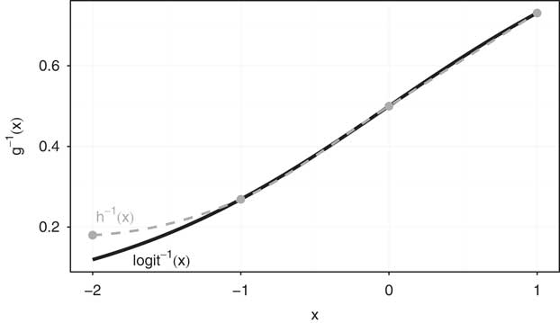
Our goal is to replace the function logit−1 with a new function h −1 to obtain Panel A of Table 1 with parameters (β, γ)=(1, −1). The only time we use logit−1(−2) in the calculation is for the bottom-right cell. In that case, let h −1(x)=logit−1(x) for x∈c{−1, 0, 1}. This ensures that all but the bottom-right cell remains unchanged. Then we require that
 $$\eqalignno{ h^{{{\minus}1}} \left( {{\minus}2} \right)h^{{{\minus}1}} \left( 1 \right) & \,{\equals}\,0.13, \cr h^{{{\minus}1}} \left( {{\minus}2} \right) {\rm log it}^{{{\minus}1}} \left( 1 \right) & \,{\equals}\,0.13, \cr h^{{{\minus}1}} \left( {{\minus}2} \right) & \,{\equals}\,{{0.13} \over {\log} {{\rm it}^{{{\minus}1}} \left( 1 \right)}}, \cr h^{{{\minus}1}} \left( {{\minus}2} \right) & \,{\equals}\,{{0.13} \over {0.73}}, \cr h^{{{\minus}1}} \left( {{\minus}2} \right) & \,{\equals}\,0.18\,\left( {{\rm as}\,{\rm opposed}\,{\rm to}\,{\rm logit}^{{{\minus}1}} \left( {{\minus}2} \right)\,{\equals}\,0.12} \right). $$
Figure 1 compares the functions logit−1 and h −1, which are similar, yet lead to exactly opposite inferences about the effects of x on d main and d nuisance. If the researcher obtains a large set of data with proportions identical to Panel A of Table 1, then her conclusion about the effects of x on d main and d nuisance depends on her assumption about the link function. If she assumes the logit link function, then she concludes that x has a large, negative effect on d main. If she assumes the link function h, then she concludes that x has a large, positive effect on d main. This example clearly highlights how minor errors in model specification can lead to large bias. To show the potential for bias in a broader collection of situations, we now turn to two simulation studies.
The link functions logit−1 and h −1 that lead to exactly opposite inferences in the stylized partial observability model

Simulation Studies
We use two simulation studies to support our claim that partial observability models are highly sensitive to seemingly innocuous specification errors. In the first study, we evaluate the bias in the partial observability logit model estimates as the link function g of the true data-generating process (DGP) varies. We view this as a highly conservative test of our claim, but find that misspecifying the link function can lead to large biases. In the second study, we consider more realistic, but still conservative misspecifications of the functional form. Berry, DeMeritt and Esarey (2015) observe that few social science theories offer more precision than a simple monotonic relationship between an explanatory variable and the probability of an event. Motivated by their observation, we evaluate the performance of the partial observability logit model for a variety of monotonic DGPs. The simulations clearly show that (1) neither type of misspecification introduces much bias into the estimate under full observability and (2) both types of misspecification can introduce large bias into the estimate under partial observability, including sign errors.
Simulation Study 1: Wrong Link Function
Many researchers view the choice of link function in a model of a binary outcome as an arbitrary, unimportant choice. Berry, DeMeritt and Esarey (2015) summarize this idea:
In the typical study using binary logit or probit, the theory introduced is not sufficiently specific to imply that logit, probit, or any other functional form is a good fit to the hypothesized DGP. Instead, logit or probit is chosen from among the countless possible functional forms for a model simply because logit and probit have come to be viewed as “default” estimators for a binary dependent variable model—making them convenient estimation choices.
We endorse and echo the authors’ key point: in the social sciences, researchers rarely have a strong theoretical justification for choosing one functional form over another.
Given that researchers seldom have a compelling reason to prefer a logit model over a probit model, a cloglog model, or a cauchit model, we would find it especially troubling if the ability of the partial observability model to recover the quantity of interest depends on the researcher choosing the proper link function. Our simulations show exactly this—if the researcher chooses the wrong link function (e.g., uses a partial observability logit model for a cauchit DGP), then the large-sample estimates can have substantial bias.
To assess the large-sample bias of the partial observability model we simulate 500 large data sets for each of our DGPs (i.e., 100 million observations for each unique combination of the values for each explanatory variable). Across each data set, we randomly vary k w (the number of variables explaining both d main and d nuisance), k x (the number of variables explaining only d main), k z (the number of variables explaining only d nuisance), β (the coefficients in the model of d main), and γ (the coefficients in the model of d nuisance). The parameters are drawn from the following distributions:
 $$\eqalignno{ k_{w} {\minus}1 & \,\sim\,{\rm Poisson}\left( {0.5} \right), \cr k_{x} & \,\sim\,{\rm Poisson}\left( {1.5} \right), \cr k_{z} & \,\sim\,{\rm Poisson}\left( {1.5} \right), \cr \beta ^{{\asterisk}} & \,\sim\,{\rm uniform}\left( {{\minus}1,\,1} \right), \cr \gamma ^{{\asterisk}} & \,\sim\,{\rm uniform}\left( {{\minus}1,\,1} \right). $$
We also randomly vary the type of each explanatory variable, either binary or continuous, so that each variable is binary with probability 0.5. For computational ease, continuous variables take on values 0.0, 0.2, 0.4, 0.6, 0.8, or 1. For each random set of simulation parameters, we simulate a large data set using logit, probit, cloglog, and cauchit DGPs. For each DGP, we rescale the coefficients β * and γ * so that the true first differences are approximately equal across DGPs. For each data set, we use the partial observability logit model to estimate the first difference as the key explanatory variable w 1 varies from its minimum to its maximum (i.e., 0–1). First section of the Online Appendix summarizes the details of the algorithm.
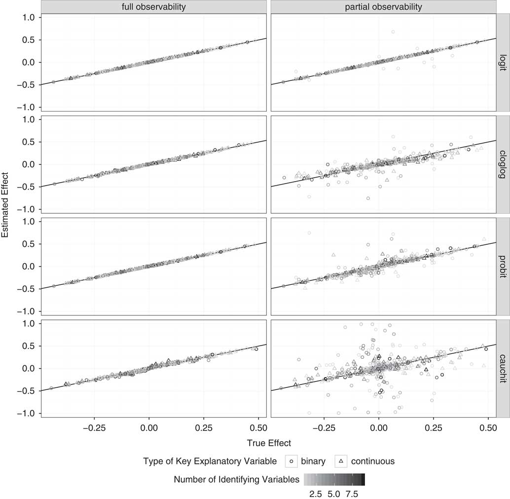
Figure 2 shows the large-sample estimates of the first difference. The left-hand column shows the relationship between the estimated effect and true effect under full observability, where misspecifying the link function has almost no effect on the inferences. The largest biases under full observability occur for the cauchit DGP, where the average absolute bias is <0.01. The average absolute true effect is about 0.1, so the average absolute bias is relatively small. Most importantly, though, the estimate almost always falls close to the true value regardless of the DGP. For the worst-case cauchit DGP, the 95th percentile of the absolute bias is about 0.04 and the maximum is 0.08. The correlations between the estimated effect and the true effect for a cauchit DGP is 0.99. We would expect any biases to be minor; the cauchit link function is nearly indistinguishable from the logit link function and there is almost never a compelling theoretical reason to prefer one over the other.
The large-sample estimates of the first difference as the true first difference varies Note: The left column shows the estimates under full observability (i.e., usual logit model) and the right column shows the estimates under partial observability. The top row shows the estimates when the link function is specified correctly as logit. The remaining rows show the estimates when the link function is not specified correctly (i.e., specified as logit when the data-generating process is probit, cloglog, and cauchit).

The results under partial observability, though, tell a different story—the bias can be much larger. For the cauchit DGP, the average absolute bias is about 0.07 when w 1 is continuous and about 0.20 when w 1 is binary—about 7 and 20 times larger under partial observability than under full observability, respectively. Under partial observability, the correlation between the estimated effect and the true effects drops to 0.69 when w 1 is continuous and to 0.32 when w 1 is binary. And remember that standard errors do not reflect this large-sample bias and that the bias does not shrink as the sample size increases. This performance differential does not occur because the partial observability model requires more information to estimate the parameters; it occurs because the partial observability model is highly sensitive to misspecification.
Unlike the full observability model, the partial observability model does not guarantee an estimate close to the true value. For the cauchit DGP, the 95th percentile for the average absolute bias is about 0.17 and the maximum is about 0.30 when w 1 is continuous. When w 1 is binary, the 95th percentile is 0.83 and the maximum is 1.12. Though the researcher has made only a small specification error, this small error produces a moderate-to-large bias on average and an enormous bias on occasion. Perhaps most informatively, for the cauchit DGP, the partial observability logit model produces sign errors in 24 percent of the simulations when w 1 is continuous and in 31 percent of the simulations when w 1 is binary. That is, when using a partial observability logit model to estimate a cauchit DGP, not only does the estimate converge to the wrong value (i.e., is inconsistent), it often converges to a value with the wrong sign! In contrast, the full observability logit model does not produce a single sign error in our simulations, regardless of the DGP.
While the cauchit DGP acts as the worst-case scenario for the partial observability logit model, the biases that emerge for the probit DGP are especially telling. The conventional wisdom suggests that the choice between a logit and probit model is inconsequential. Indeed, King (1998, 100) notes in passing that the two link functions “produce almost identical inferences in practical social science problems.” This claim holds in the context of full observability (where King makes the claim), but the partial observability logit model estimates can have substantial bias under a probit DGP. For example, the average absolute bias in the estimates of the partial observability logit model for a probit DGP is about 0.03 for both a continuous and a binary w 1, which is about three times the worst-case scenario under full observability. Perhaps more importantly, the partial observability model has a much higher likelihood of substantial large-sample bias than the full observability model. The 95th percentile of the absolute bias is 0.12 and the maximum is 0.35 when w 1 is continuous. When w 1 is binary, the 95th percentile is 0.12 and the maximum is 0.55. About 4 percent of the simulations produce a sign error. While this potential for bias might be small enough or rare enough to ignore, these results highlight the bias that even minor errors in the functional form can produce.
Lastly, notice that substantial large-sample bias does not only occur among models with one or two identifying variables. For the probit DGP, increasing the number of identifying variables (n x +n z ) from one to four shrinks the 95th percentile of the absolute bias from about 0.15 to about 0.10. For the cloglog DGP, this same change shrinks the 95th percentile from 0.21 to 0.15. For the cauchit DGP, the 95th percentile shrinks from 0.73 to 0.69. Even with several identifying variables, the potential for bias remains quite large.
Whereas the full observability logit model can estimate the first difference accurately whether the true DGP is logit, probit, cloglog, or cauchit, the partial observability logit model performs noticeably worse for the probit, cloglog, and cauchit DGPs. In particular, a functional form mismatch leads to moderate-to-large bias on average and dramatically raises the likelihood of an enormous bias, including sign errors. But we view this first study only as a heuristic to illustrate the extreme sensitivity of the partial observability model. In our second simulation, we turn to a more realistic scenario with more general, monotonic DGPs.
Simulation Study 2: A Monotonic Relationship
Our second simulation study mirrors that of Berry, DeMeritt and Esarey (2015). In these simulations, we assume that the researcher uses the partial observability logit model to estimate a first difference when the DGP is actually some monotonic relationship among the explanatory variables and the probability of an event, so that
 $$\eqalignno{ & {\rm Pr}\left( {d_{{{\rm main}}} } \right)\,{\equals}\,p\left( w \right), \cr & {\rm Pr}\left( {d_{{{\rm nuisance}}} } \right)\,{\equals}\,q\left( {w,\,z} \right), \cr & {\rm Pr}\left( {y_{{{\rm obs}}} } \right)\,{\equals}\,{\rm Pr}\left( {d_{{{\rm main}}} } \right){\rm Pr}\left( {d_{{{\rm nuisance}}} } \right), $$
where p and q are monotonic functions of x and x and z, respectively.
In our view, even the strongest social science theory will not specify the exact functional form relating the explanatory variables to the unobserved outcomes. However, a good theory might specify a monotonic relationship between the explanatory variables and the probability of an event.
In this simulation, the relationships are monotonic and the researcher includes the variables in the appropriate equations, so the misspecification, while always present, remains slight. We view this study as a more realistic, but still conservative evaluation of the partial observability model. While the deviation from the typical link functions (logit, probit, cloglog, cauchit, etc.) can be quite large in this simulation, two features work in favor of the partial observability model. First, we place the variables w and z in the correct equations. In applied research, the researcher must usually make these choices guided only by relatively weak theory. Second, we allow the effects of the identifying variable z to be quite large. In applied work, the researcher might rely on one or more variables that have relatively small effects.
Indeed, this strikes us as a realistic, but best-case scenario for social science research. Following Berry, DeMeritt and Esarey (2015), we simulate a pool of 2000 DGPs that meet the monotonicity condition, where each true DGP can be represented by the nonlinear, interactive equations
 $$\eqalignno{ & \left. {{\rm Pr}\left( {d_{{{\rm main}}} } \right)} \right\,{\equals}\,\beta _{{{\rm cons}}} {\plus}\beta _{w} w{\plus}\beta _{{w^{2} }} w^{2} , \cr & {\rm Pr}\left( {d_{{{\rm nuisance}}} } \right)\,{\equals}\,\gamma _{{{\rm cons}}} {\plus}\gamma _{w} w{\plus}{\plus}\gamma _{z} z{\plus}\gamma _{{w^{2} }} w^{2} {\plus}\gamma _{{z^{2} }} z^{2} {\plus}\gamma _{{wz}} wz, \cr & {\rm Pr}\left( y \right)\,{\equals}\,{\rm Pr}\left( {d_{{{\rm main}}} } \right){\rm Pr}\left( {d_{{{\rm nuisance}}} } \right). $$
To choose the coefficients, β and γ are drawn from a uniform(−1, 1) distribution. Values that do not meet the monotonicity condition are discarded.
As before, we simulate a large data set (i.e., 100 million observations) for every possible combination of covariate values for each DGP. We use this data set to estimate the full and partial observability logit models. Finally, we compare these large-sample estimates of the quantity of interest to the true value. As before, we focus on the ability of the partial observability model to recover the change in the probability of d main as w moves from its minimum to its maximum (0, 1). Second section of the Online Appendix summarizes the details of the algorithm.
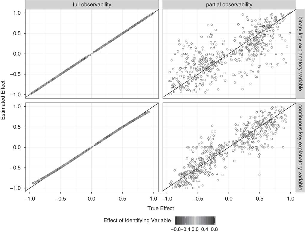
Figure 3 shows the results. The left-hand column shows the full observability logit model estimates of the first difference. These estimates are extremely accurate when w is binary. This occurs because the logit model can perfectly represent the probability of an event, regardless of the “functional form” when the single explanatory variable w is binary. This is not the case for the continuous w, though. In spite of the fact that the full observability model might only roughly approximate p(w), the bottom left-hand panel of Figure 3 shows that the full observability model can estimate the effect of w on Pr(d main) extremely well.
The large-sample estimates of the first difference as the true first difference varies Note: The left column shows the estimates under full observability (i.e., usual logit model) and the right column shows the estimates under partial observability. The top row shows the estimates when the key explanatory variable is binary and the bottom row shows the estimates when the key explanatory variable is continuous.

Though the functional form misspecification has almost no influence on the ability of the full observability logit model to estimate the effect of interest, the same misspecification causes substantial bias in the partial observability estimates. For a continuous w, the average absolute bias is about 0.19. The 95th percentile is 0.54, and the maximum bias in our sample is 1.17. For a binary w, the average absolute bias is 0.28, the 95th percentile is 0.85, and the maximum is 1.15. The large-sample absolute bias is >0.1 in 65 percent of the simulations, >0.3 in 27 percent of the simulations, and >0.5 in 12 percent of the simulations. To put this in perspective, many effects of interest to political scientists are <0.1.
Sign errors are also a substantial problem for the monotonic DGP. When w 1 is binary, 19 percent of the simulations produce a large-sample sign error. When w 1 is continuous, this only shrinks to about 11 percent. In applied settings, not only do researchers need to worry about sampling error, they need to worry that the model, even with negligible sampling error, may converge to an estimate with the wrong sign.
One might suspect that the magnitude of the bias depends on the magnitude of the effect of the identifying variable. As the magnitude of the effect of the identifying variable increases, the potential for bias does tend to decrease, but it shrinks rather slowly. The 95th percentile of the absolute bias is 1.00 when the effect of z is 0.1. If z has a much larger effect of 0.5, then the 95th percentile of the absolute bias only drops to 0.58.
Conclusion
We highlight an under-appreciated but critical characteristic of partial observability models—they are quite sensitive to seemingly innocuous specification errors. Even small errors in the functional form can lead to a substantial bias in large samples, including sign errors.
Meng and Schmidt (Reference Meng and Schmidt1985) counseled economists early on regarding some of the costs of partial observability, arguing that standard errors are much larger when the outcome of interest is only partially observed. They write, “we would not be surprised to find, in a typical application, t-ratios to be from two to four times as large under full observability as under partial observability” (Meng and Schmidt Reference Meng and Schmidt1985, 83). Yet by design, standard errors only reflect the uncertainty due to sampling error. Other sources of error, such as measurement error, missing data, and specification error create additional uncertainty. In the case of full observability, our simulations show that the functional form has a negligible impact on the large-sample estimates. But in the case of partial observability, uncertainty about the functional form should generate suspicion about the estimates. The bias introduced from specification error of the partial observability model can be quite large, is rarely negligible, and is not captured in the standard errors.
What about the possibility of model specification tests to determine the severity of the misspecification? We are not optimistic about this possibility. The motivating example shows that two models can fit the observed data exactly and still provide opposite inferences. In general, researchers could use a test to determine whether the partial observability model offers a good model of Pr(y obs). But researchers cannot evaluate the quality of the models of Pr(d main) and Pr(d nuisance) because these variables are unobserved. A model might predict the observed data quite well, but offer terrible predictions for the unobserved data. Thus, specification tests cannot resolve the issue when the researcher is interested in explaining d main.
Recent applications are relatively sanguine about employing the partial observability model. For example, Przeworski and Vreeland (Reference Przeworski and Vreeland2002) (see also Przeworski and Vreeland Reference Przeworski and Vreeland2000; Vreeland Reference Vreeland2003; Stone Reference Stone2008) are interested in how surplus in a nation’s budget affects both the IMF’s and the national government’s decisions to enter an agreement. They find that, as a budget surplus increases, a government becomes less likely to enter an IMF agreement, but the IMF becomes more likely to enter an agreement. Interestingly, and consistent with our claim, Stone (Reference Stone2008) uses data from a later time period and reports an opposite effect of the budget surplus on a government’s decision to participate in an agreement. In spite of these and other optimistic applications of the partial observability model, our analysis suggests that skepticism is in order. Indeed, our simulations show that relatively minor and unavoidable model specification errors can lead to a substantial large-sample bias in the estimates. In our view, no easy methodological fix exists. Instead, we encourage scholars to view partial observability estimates with skepticism and encourage researchers to collect more complete data, directly observing the outcome of interest.